Dynamic Moduli and Poisson’s Ratios in Experiments with Fluid-Saturated Porous Rock

Igor B. Morozov

Abstract

The concept of dynamic (frequency-dependent) viscoelastic modulus is broadly used for describing mechanical properties of rocks and building attenuation and fluid-substitution models. However, for porous rock saturated with fluids, this concept is approximate and does not reproduce the stress fields within seismic waves and boundary conditions between contrasting media. Consequently, for heterogeneous poroelastic media, calculations based on a single effective P-wave modulus may often be inaccurate or incorrect. To examine the accuracy of the viscoelastic approximation, we use Biot’s theory to compare the P-wave and Young’s moduli for traveling waves and extensional subresonant laboratory measurements with short cylindrical specimens. Four observations are made from this comparison. First, for seismic waves, the moduli measured from stress/strain ratios differ from those determined from wave velocity and attenuation. The differences between these quantities are mainly in the strength of dispersion and poroelastic dissipation. Second, for the waves, the dynamic P-wave and Young’s moduli and the Poisson’s ratios do not obey the mutual relations usually expected from (visco)elastic moduli. Third, the moduli measured from stress/strain ratios in the laboratory differ from those for traveling waves. In a cylindrical specimen, frequency effects occur at much lower (10–100 times) frequencies than the dissipation peaks in traveling waves. Fourth, the moduli and particularly attenuation measured in short cylinders depend on the lengths of the specimens. All these observations are caused by the contributions of secondary P-wave modes to the deformations of small specimens. To account for these contributions, dynamic moduli need to be considered for all primary and secondary wave modes within the body. An alternate and better approach could consist in using first-principle physics for describing the material and boundary conditions of the specific experiment. Qualitatively, these conclusions should also apply to the more general wave-induced flow effects in fluid-saturated porous rock.

2

Introduction

Estimation of mechanical properties of fluid-saturated porous rock from observations of wave attenuation and dispersion is among the primary goals of seismic studies. Numerous field and laboratory data show that pore-space and pore-fluid properties affect the velocities and attenuation of seismic waves as well as on reflectivity (e.g., Müller et al., 2010; Lines et al., 2014). The measurements, modeling and inversion of such effects for petrophysical properties of reservoir and crustal rock commonly utilize the concept of dynamic (complex-valued and frequency-dependent) bulk and shear moduli. These moduli combine the observed characteristics of wave propagation within the rock, such as the wave speeds and quality factors, Q. Frequency dependences of these moduli are approximated by empirical relations such as the Andrade or Cole-Cole laws (Cooper, 2002; Adam et al., 2009) or models of linear solids (Liu et al., 1976).

In practical studies, the dynamic modulus is often treated as a fundamental intrinsic property of the rock, or at least some combination of its properties responsible for wave speed and energy dissipation (e.g., Batzle et. al, 2014). The complex argument of the modulus is often interpreted as an inherent stress/strain phase lag and serves for designing and interpreting attenuation experiments at seismic frequencies (Jackson and Paterson, 1993; Lakes, 2009; Tisato and Madonna, 2012). However, the existence and uniqueness of such a combination is still not guaranteed, and it is also not always needed for explaining the obserrvations. The most rigorous and developed macroscopic models of internal friction within solids, such as poroelasticty (Biot, 1962), viscosity and thermoelasticity (Landau and Lifshitz, 1986) – do not rely on the moduli. The moduli-based viscoelastic model implies certain assumptions and represents an approximation whose accuracy needs to be examined in each specific case.

The goal of this paper is to check how the viscoelastic approximation works for the poroelastic mechanism at low (seismic) frequencies. We try answering whether the effective viscoelastic modulus or some other physical parameters of a poroelastic material represent a sufficient and reliable characterization of its mechanical properties. Clearly, knowing such parameter(s) is critical for interpreting wave-propagation and attenuation experiments and models.

Poroelasticity is an important attenuation mechanism in itself, and it also possesses important similarities (two-constituent structure, microstructural heterogeneity, mobile and viscous pore fluids) with a broad group of wave-induced fluid flow mechanisms (WIFF). WIFF mechanisms are considered the primary cause of seismic attenuation in sedimentary rocks at seismic frequencies (Müller et al., 2010). Fluid-flow effects are especially strong for patchy saturations (White, 1975; Johnson, 2001). Recently, realistic 2-D and 3-D models of heterogeneous saturations were studied numerically (Rubino and Holliger, 2012) and compared to laboratory observations (Kuteynikova et al., 2014, and references therein). In these studies, the principal quantities used to connect the modeling to observations were again the dynamic Young’s and P-wave moduli. Thus,

3

understanding of the character of dynamic moduli for fluid-flow related internal friction is important for interpreting the observations of WIFF.

In comparing the poroelastic and viscoelastic predictions, we do not consider the effects of grain sizes, multiple saturation fluids, patchy saturations and other WIFF effects, and also the upscaling of laboratory observations to field conditions. We focus on only two questions related to the macroscopic boundary conditions of the experiments:

i) Do the complex-valued empirical moduli measured at low frequencies in experiments with traveling waves equal those measured in short cylindrical rock specimens?

ii) Do these moduli obey the relations usually expected from the (visco)elastic moduli? This question applies to the mutual relations between the different moduli as well as to the relations of the moduli to wave velocities and acoustic impedances.

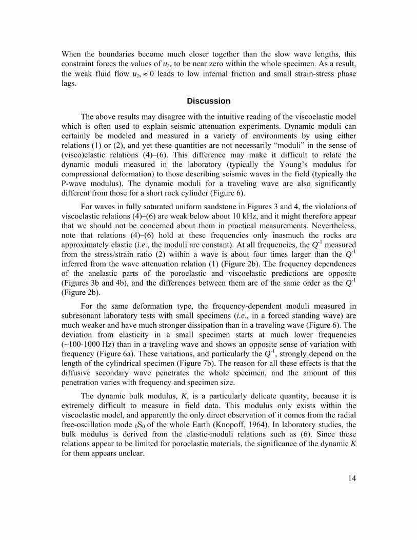
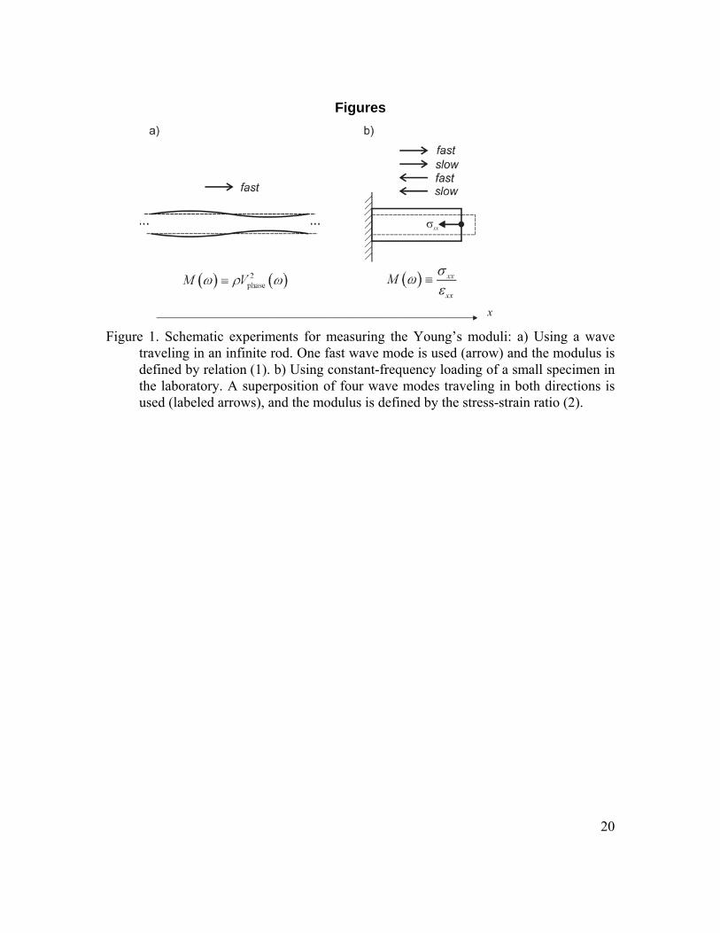
To answer these questions, we derive the P-wave and Young’s moduli and the Poisson’s ratio for propagating P waves and for an experiment with subresonant extensional-mode deformation of a rock cylinder (Figure 1). Dunn (1986) considered similar experiments with emphasis on the “anomalous attenuation” resulting from an open-pore surface of the cylinder. In this paper, we only consider impermeable boundaries and axial deformations.

The results show that if we try describing a poroelastic material by a single dynamic P-wave modulus (as commonly done), the answers to the questions i) and ii) are generally negative. Our general observations are:

1) At nonzero frequencies, the empirical P-wave (M) and Young’s (E) moduli for a cylindrical rock specimen are significantly lower than the corresponding Mfast and Efast for a propagating wave. The relations between M, E, Mfast, and Efast are nontrivial and frequency-dependent, and they do not follow the conventional relations for the elastic moduli.

2) The stress-strain phase lags measured in a rock specimen are strongly affected by Biot’s slow P wave. Because the slow-wave length is close but longer than the dimensions of the specimen, its distribution within the cylinder is influenced by the boundary conditions on all surfaces of the specimen. Consequently, the shape and dimensions of the specimen affect the empirical stress/strain ratios, i.e. moduli.

Dunn (1986) also noted the dependence of the complex argument of the dynamic modulus (Q-1) on the boundary conditions on the surface of the cylinder. For internal friction caused by nonlinear solid viscosity, similar observations were made by Coulman et al. (2013).

Thus, the dynamic moduli measured by using traveling and standing waves in experiments of different geometries may be difficult to relate to each other. The reason for this is easy to see: in a finite poroelastic body (and also in bodies with WIFF; cf.

4

Dutta and Odé, 1979a), multiple wave modes are always present even in the simplest laboratory experiment. A consistent characterization of the material would therefore require defining the moduli for all primary and secondary waves and determining the relative amplitudes of these waves in each experiment. However, establishing the modal content can be complicated for bodies of complex shapes.

In the following section, we briefly summarize the general properties expected from a dynamic modulus and the two general types of moduli measured from field and laboratory data. These overviews show that the wave-mode content and the measurement procedure always influence the observed value of the dynamic modulus. In the last two sections, we numerically model the low-frequency moduli measured in 1-D, traveling waves and short cylindrical sandstone specimens.

Along with noting the properties of the poroelastic dynamic moduli, the models below show how the field and laboratory experiments can be interpreted without relying on the dynamic moduli. In a first-principle physical approach, the material is described by three local and matrix-valued constitutive properties: density, rigidity and Darcy friction. The experiments are modeled in their specific geometries, by directly using the differential equations of continuum mechanics.

The dynamic modulus

Expected properties

Describing the elastic and anelastic responses of a rock body by a dynamic modulus is not merely a convenient way for communicating the results of observations. Recognition of a quantity called “modulus” implies certain general properties of the mechanical behavior of the body:

1) The modulus is expected to be a property of the material and at least relatively insensitive to “extrinsic” parameters of the experiment, such as the shape and dimensions of the specimen. On the other hand, dependences on “intrinsic” parameters such as the frequency, pressure, fluid distribution, and temperature may be allowed.

2) The moduli derived for different shapes of deformation (for example, P-wave, Young’s, bulk, and shear) are expected to follow their mutual relations known from elasticity.

3) In experiments with waves, the moduli are also expected to be related to wave speeds and attenuation factors (Q-1).

4) In experiments with forced oscillations of material samples in the laboratory and also in seismic waves, the moduli must also equal the appropriate ratios of stresses to strains.

5) To be useful for predicting seismic reflection amplitudes in layered media, the moduli should also reproduce seismic impedances, for example, as

5

/Z p v M , where p is the pressure within the wave, and v is the

particle velocity with it, M is the P-wave modulus, and is the density (Aki and Richards, 2002).

Properties 3) and 4) are the basis for two approaches to measuring the moduli, property 2) is often used for extracting the desired moduli from the observed ones (such as the P-wave or bulk from the Young’s modulus; e.g., White, 1965), and property 1) is critical for relating the results to the physical state of the material.

As shown below, the above properties mutually disagree for a poroelastic material at nonzero frequencies. This disagreement occurs because the pore-fluid friction is physically distinct from viscosity and elasticity, despite producing spectral attenuation peaks similar to those of a Standard Linear Solid (Geertsma and Smit, 1961). In contrast to viscosity, the internal friction within a poroelastic medium is caused not by gradients of deformation velocities (strain rates) but by the relative velocities between the solid and fluid phases (Darcy’s or Biot’s friction). Unlike the elastic and viscous forces, this friction is not a surface but body force which is more analogous to an effect of inertia than that of a modulus. This force does not contribute to the pressure and boundary conditions between contrasting media, and consequently property 5) above is particularly problematic. As shown by Morozov (2011), with body-force friction, reflections from pure Q-contrasts have opposite polarities compared to the viscoelastic predictions.

The dynamic modulus is also sensitive to the measurement procedure (property 1 above). It is well known that different moduli correspond to bulk and shear deformations, and these moduli also vary with frequency. However, frequency is not the only experimental factor affecting the measurements. For a saturated porous rock, another key factor is the relative contributions of the primary (“fast”) and secondary (“slow”) Biot’s P waves. Each of these waves possesses a dynamic P-wave modulus that we denote Mfast and Mslow and that are strongly different. In observations with uniform media, Mfast is of primary interest because the slow wave is diffusive and only present near boundaries. However, in experiments with small rock specimens, the measured modulus (which we denote Mstand) belongs to neither of these modes but to a standing wave. As shown below, the relation of Mstand to Mfast and Mslow is nontrivial and controlled by the shape and dimensions of the specimen and by the frequency. For the next section, it is most important that Mstand Mfast for short specimens.

Viscoelastic relations

The dynamic modulus plays two distinct roles in describing the mechanical properties of the medium. First, in observations of seismic waves, the “wave” modulus is measured from the wave velocity:

*2phaseM V , (1)

where is the density, is the angular frequency, and

6

* 1phase phase 1 2V V i Q is the complex-valued phase velocity (Figure 1a).

The practical meaning of this modulus is in comprising the phase velocity and attenuation of the wave. However, in a laboratory experiment with a small specimen of fluid-saturated rock, definition (1) cannot be used directly, because fast and slow waves traveling in both directions are present within the specimen (Figure 1b). Therefore, the P-wave modulus measured for the cylinder represents some mixture of Mfast and Mslow. To measure this modulus, a different form is used for M(), giving M as the ratio of the applied axial stress, xx, to the average strain in the specimen, xx (e.g., White, 1965; Jackson and Paterson, 1993):

xx

xx

M

. (2)

Along with the frequency, this ratio may in principle depend on other experimental parameters, such as the shape and length of the specimen. Since most laboratory experiments do not permit significant variations in the dimensions of the specimens, these dependences need to be studied theoretically.

Expressions (1) and (2) are automatically equal only within the viscoelastic model, which assumes that the internal friction is indeed due to a complex modulus in the frequency domain. This means that the frictional stress field is proportional to the strain and spatially isomorphic to that in Newtonian viscosity (page 849 in Ben-Menahem and Singh, 1981), which in its turn, is isomorphic to the elastic stress:

friction Im 2 Imij ij kk ij . (3)

Such form of the frictional stress is only observed in linear solid viscosity, in which Im and Im , where is the viscosity and is the second viscosity

(Landau and Lifshitz, 1986). However, for constant and , this model predicts a Q factor strictly proportional to 1/, which is usually not the case for rocks. Moreover, in a poroelastic medium, frictional forces do not follow the tensor relation (3) at all (see eq. (8) below).

To test the relations (1) and (2) for a fluid-saturated porous rock, consider an experiment with subresonant axial deformation of a cylindrical rock specimen, such as by Tisato and Madonna (2012) or Batzle et al. (2014) (Figure 1b). To measure the P-wave modulus by using relation (2), the cylinder must be extended or compressed along its axis X so that it does not deform in the directions Y and Z, i.e. the transverse strain equals zero: yy = zz = 0. However, such boundary condition is difficult to implement, and cylinders with free transverse boundary are usually used, i.e. with zero perturbation of the stress: yy = zz = 0. In this case, the stress/strain ratio (2) represents the Young’s modulus, which we denote E(). In most materials, E < M because of the transverse

7

thickening of the cylinder upon axial compression. This thickening is characterized by the Poisson’s ratio:

2

2yy

xx

M

M

. (4)

The second equation in (4) is valid for an elastic solid, and in the viscoelastic model, this relation is extrapolated to the anelastic case (Tschoegl et al., 2002; Lakes and Wineman, 2006). Similarly, to infer the dynamic M() from the measured E(), it is usually assumed that these quantities obey the relations for elastic moduli (White, 1965):

3EM

, and conversely, 3

ME

, (5)

where is the shear modulus. If the Poisson’s ratio can be measured, then the anelastic shear and bulk moduli can also be derived from E by assuming that they are related as elastic ones:

3 1

E

and 3 1 2

EK

. (6)

From each of the above complex-valued moduli, the respective Q-factors are extracted as (ibid):

1P

Im

Re

MQ

M , 1 Im

ReE

EQ

E , 1

S

Im

ReQ

, and 1 Im

ReK

KQ

K , (7)

with elaborate relations resulting between these Q-factors and seismic wave speeds (Knopoff, 1964). The relations (2)–(6) constitute the correspondence principle, which states that the solution of an anelastic problem can be obtained from the elastic one by extrapolating the elastic moduli into the complex domain and making them frequency-dependent (Ben-Menahem and Singh, 1981; Lakes, 2009).

For porous, fluid-saturated rock, relations (2)–(6) still contain two important problems. First, as shown in the next section, for a wave in a poroelastic medium, the stress/strain ratio (2) does not generally equal the density-velocity product (1). This means that the correspondence principle does not hold in this case. As mentioned above and derived in Appendix A, the difference between quantities (1) and (2) occurs because of the pore-fluid friction being body force and not a surface stress implied in (2) and (3). Second, for an anelastic rock at frequencies > 0, relations (4)–(6) between the different types of moduli only follow from a verbal interpretation of the stress-strain ratio (2) as a “modulus”. This interpretation is not automatic and needs to be verified by rigorous analysis. However, even before starting such analysis in the following sections, it seems clear that the friction of the fluid sloshed through pores or cracks is governed by

8

completely different physics and should unlikely obey the relations between the elastic moduli. Relations (4)–(6) are only guaranteed at frequency = 0, at which the pore-fluid flows are absent and the rock is elastic.

P-wave and Young’s moduli in poroelastic models

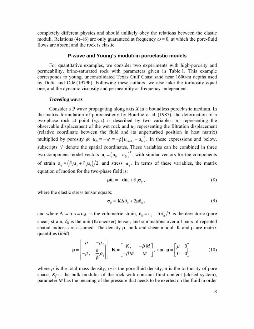
For quantitative examples, we consider two experiments with high-porosity and permeability, brine-saturated rock with parameters given in Table 1. This example corresponds to young, unconsolidated Texas Gulf Coast sand near 1600-m depths used by Dutta and Odé (1979b). Following these authors, we also take the tortuosity equal one, and the dynamic viscosity and permeability as frequency-independent.

Traveling waves

Consider a P wave propagating along axis X in a boundless poroelastic medium. In the matrix formulation of poroelasticity by Bourbié et al. (1987), the deformation of a two-phase rock at point (x,y,z) is described by two variables: u1i representing the observable displacement of the wet rock and u2i representing the filtration displacement (relative coordinate between the fluid and its unperturbed position in host matrix)

multiplied by porosity : 2 fluid, 1i i i iu w u u . In these expressions and below,

subscripts ‘i’ denote the spatial coordinates. These variables can be combined in three

two-component model vectors 1 2

T

i i iu uu , with similar vectors for the components

of strain 2ij i j j i ε u u and stress ijσ . In terms of these variables, the matrix

equation of motion for the two-phase field is:

i i j ij ρu du σ , (8)

where the elastic stress tensor equals:

2ij ij ij σ KΔ με , (9)

and where tr kk is the volumetric strain, 3ij ij ij ε ε Δ is the deviatoric (pure

shear) strain, ij is the unit (Kronecker) tensor, and summations over all pairs of repeated spatial indices are assumed. The density , bulk and shear moduli and are matrix quantities (ibid):

f

f f

a

ρ , fK M

M M

K , and 0

0 0

μ . (10)

where is the total mass density, f is the pore fluid density, a is the tortuosity of pore space, f is the bulk modulus of the rock with constant fluid content (closed system), parameter M has the meaning of the pressure that needs to be exerted on the fluid in order

9

to increase the fluid content by a unit value at constant volume, parameter [0, 1] measures the proportion of the apparent macroscopic dilatational strain caused by variations in fluid content, and is the shear modulus. All these physical parameters are measurable in a set of properly designed quasi-static experiments and lead to Gassmann’s equations (ibid). The matrix d in equation (8) describes the friction caused by the volumetric pore flow (ibid):

0 0

0

d , (11)

where is the permeability of the rock, and is the viscosity of the pore fluid. Note that all quantities (10) and (11) are specified before any oscillatory motion is considered within the medium, and consequently they represent true medium properties.

For a plane P wave, all displacements are oriented in the direction of the spatial axis X: 1Jk J ku u , where the upper-case subscript J =1,2 enumerates the above model

variables and the lower-case subscripts refer to spatial coordinates. The strain tensor therefore equals 1 1Jik J i ku , where the prime denotes the spatial derivative with

respect to the coordinate x. The equation of motion (8) then simplifies to:

ρu du Mu , (12)

where 4 3 M K μ is the matrix P-wave modulus.

Further, let the wave be harmonic in time and exponentially decaying in space:

exp i t ikx x u A , (13)

where A is the vector amplitude (including the relative phase shifts of the two variables), is the frequency, k is the wavenumber, and is the logarithmic spatial

decrement for the amplitude. If we denote 2 2k i , equation (12) shows that

wave modes (n) are eigenvectors of the following generalized eigenvector problem (equation (A17) in Appendix A):

* n nρ υ Mυ , (14)

where the “complex density” matrix * is:

* i

ρ ρ d . (15)

Note that from equation (14), the correspondence principle for poroelasticity differs from the viscoelastic one: the moduli remain elastic (real-valued) but the density (15) becomes complex-valued and contains the internal friction.

10

Equation (14) yields two eigenvectors corresponding to plane harmonic P waves with complex phase velocities * 1V . These complex velocities comprise the phase

velocities *ReV V and quality factors * *Re 2 ImQ V V observed for the wave. The faster of these modes with k is the primary P wave, and the much slower and diffusive second mode with k is the “fluid” wave (Biot, 1962; Dutta and Odé, 1979a; Johnson, 2001).

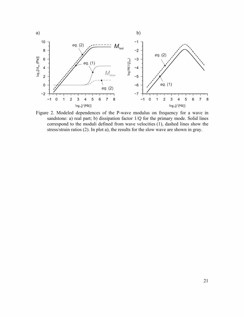
For the P-wave case, solving the eigenvalue problem (14) yields a frequency-dependent ReMfast() and a much weaker ReMslow() (Figure 2a). In this Figure, note that these quantities, which represent the “wave” moduli in relation (1) (solid lines in Figure 2a), differ from the stress-strain ratios (2) (dashed lines). For the fast mode, Figure 2b also shows the attenuation factors derived from these moduli by using relations (7). Note that the peak Q-factors differ by about four times between the wave-velocity and stress/strain ratio definitions for M (Figure 2b).

To independently evaluate the Young’s modulus (2) and the Poisson’s ratio (4) in an extensional-deformation wave, consider another experiment with an extensional wave propagating along an infinite thin rod (Figure 1a). In this case, there exists a transverse component in u1i but not in u2i, because the transverse pore-pressure gradient equals zero. Unlike in the true P-wave case, the boundary condition for the rod is 1 1 0yy zz

(recall that the first upper-case subscript here denotes the rock deformation variable J = 1). The axial components of strain are then Jxx Jxu , with J = 1, 2. In the low-

frequency approximation, 1yy is constant within the cross-section of the rod, and the

transverse displacement is proportional to the distance from the axis: 1 1y yyu y . In

Appendix B, it is shown that the transverse elastic stress equals:

1 1 1 22yy f xx f yy xxM , (16)

where 2 3f fK is the Lamé modulus of the saturated rock. The condition

1 0yy therefore requires that the transverse strain of the rod is related to the two axial

strains:

1 1 1 2 2yy x xu u and 1 1y yyu y , (17)

where 1 2f f is the elastic Poisson’s ratio (4) and 2 2 fM

is a similar ratio for equilibrium transverse thickening caused by the axial fluid flow. As shown in Appendix A, in this case, the axial deformation also obeys the eigenvalue relation (14), but with different matrices * and M.

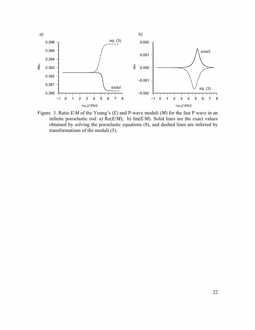
The results for a wave with free transverse boundary of the rod (Young’s modulus case) are shown in the form of E/M ratios in Figure 3. As expected in the Introduction, these ratios do not match the viscoelastic expression (5) (dashed lines in Figure 3). Thus,

11

for porous fluid-saturated sandstone at > 0, the wave-based P-wave and Young’s moduli are not bound by the viscoelastic relations.

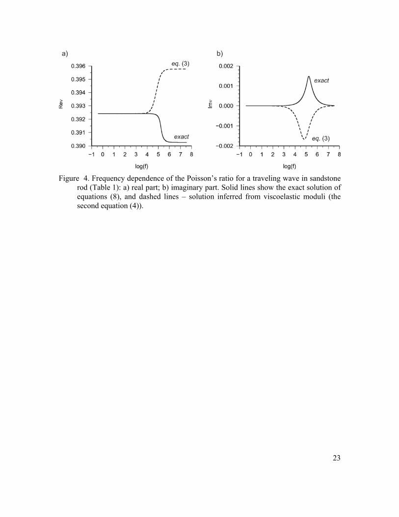
It is also interesting to plot the Poisson’s ratio (4) for a wave with a free transverse boundary (solid lines in Figure 4). For a given wave mode q(n), the Poisson’s ratio for the wave can be obtained from the ratio of the transverse and axial strains (eq. (17)):

( )

1 2( )

1 1

n

yy

nxx

EUq

EUq . (18)

In this expression, notation (…)k denotes the k-th element of the corresponding vector, and the notation for matrices E, U, and vectors q(n) is explained in Appendix A. Numerical modeling of this ratio shows that () is frequency dependent (solid lines in Figure 4) and also does not follow the viscoelastic relation (4) (dashed lines in Figure 4). Note that the variations of the Poisson’s ratio and E/M with frequency predicted by the viscoelastic approximation are opposite to those in the solution of Biot’s equations.

Axial deformation of a short cylinder

Let us now consider a short cylindrical specimen of radius R and length L, oriented in the direction of axis X (Figure 1b) and subjected to oscillatory axial compression/extension at a single, low angular frequency = 2f. We will assume that the specimen is jacketed on all sides, so that the fluid does not flow across its boundaries.

In contrast to the single, traveling wave considered in the preceding section, in the present experiment, we have a standing wave formed by an interference of forward- and backward-traveling waves. The standing wave contains both the primary (fast) and slow P waves, and consequently four wave modes are involved in this deformation. The lengths of these waves are shown as functions of frequency in Figure 5. The slow-wave modes have the largest amplitudes at the ends of the cylinder, and the depths to which they penetrate into the cylinder is the characteristic “skin depth”, which is close to its wavelength: slow slow (gray lines in Figure 5). From Figure 5, for frequencies below

about 1 kHz, both slow and slow exceed the dimensions of even the relatively large specimen in the apparatus used by Tisato and Madonna (2012) and Kuteynikova et al. (2014) (length of 25 cm and diameter 7.6 cm). Thus, in seismic-frequency laboratory experiments with sandstone, the fluid wave penetrates the whole specimen.

As an additional observation from Figure 5, note that at frequencies above the poroelastic dissipation peak, the skin depths for both fast and slow waves are nearly independent of the frequency (the difference in and between the two modes waves is also no longer pronounced at these frequencies). Such frequency independence is often observed, particularly when the attenuation is caused by geometric spreading or random scattering. Such attenuation produces an apparent Q nearly proportional to the frequency (Morozov, 2010).

12

To find the standing-wave field, we denote the amplitudes of the forward- and backward-propagating modes a+ and a–, respectively:

fast fast slow slow

fast fast slow slow

fast fast slow slow

fast fast slow slow

, (

),

ik x x ik x xi t

ik x x ik x x

x t e a e a e

a e a e

u Uq Uq

Uq Uq (19)

where vectors fast or slowq are the eigenvectors of the forward- or backward-propagating

modes of the fast or slow wave, respectively. The parameterization of these eigenvectors and matrices U producing the displacements for the different types of boundary conditions is explained in Appendix A. The relative values of a+ and a– are determined by the boundary conditions at the ends of the cylinder:

1

1

2 2

0 0 (fixed base of the cylinder),

(observed displacement),

0 0 (zero axial flow).

x

x

x x

u x

u x L L

u x u x L

. (20)

where is the desired average strain of the cylinder. These conditions lead to four equations for the amplitudes fast or slowa :

fast fast slow slow

fast fast slow slow

fast fast slow slow fast fast slow slow

fast fast slow slow

fast fast slow slow

0 (at = 0),

0

0

ik L L ik L L

ik L L ik L L

a a a a x

a e a e

La e a e

Uυ Uυ Uυ Uυ

Uυ Uυ

Uυ Uυ (at = ).x L

(21)

By solving this 44 system, we find the values of fasta , slowa , fasta , and slowa , and by

using relations (19),we obtain the distribution of rock and pore-fluid displacement within the cylinder.

For a uniaxial deformation of a sandstone cylinder, Rubino and Holliger (2012) and Kuteynikova et al. (2014) modeled the displacement fields similar to those in equations (19) by using numerical modeling. This approach allowed considering arbitrary non-uniform saturations in 2D and 3D. However, these authors only modeled the modulus M as the stress/strain ratio (2) and relied on relations (5) for transforming the measured Young’s modulus E into M as well. They also assumed that the modeled modulus is equivalent to 2

fastM V for the “fast” wave. By contrast, we examine (and

in fact, disprove) both of these assumptions by directly evaluating all measurable quantities for a uniform cylinder.

For a small specimen, the measured axial strain equals in equations (20). The confining stress measured at the end of the cylinder is given by the first element of the

13

two-element vector in expression (9) evaluated at x = L. The expressions for strain and stress within plane waves in a rod with free transverse boundaries are given in Appendix A. From equation (A19) there, the stress at the end of the cylinder is a sum of the stresses caused by each of the four wave modes (here denoted n for brevity, with n = 1…4):

( ) ( )

1 12 nik Ln n

L nn

ik e KΩUq ΕUq , (22)

where the matrices Ε and are defined in Appendix A. Note that this stress comes from purely elastic forces and includes no internal friction. Nevertheless, there still exists a phase lag between this stress and the strain, because the strain is affected by Darcy’s frictional forces.

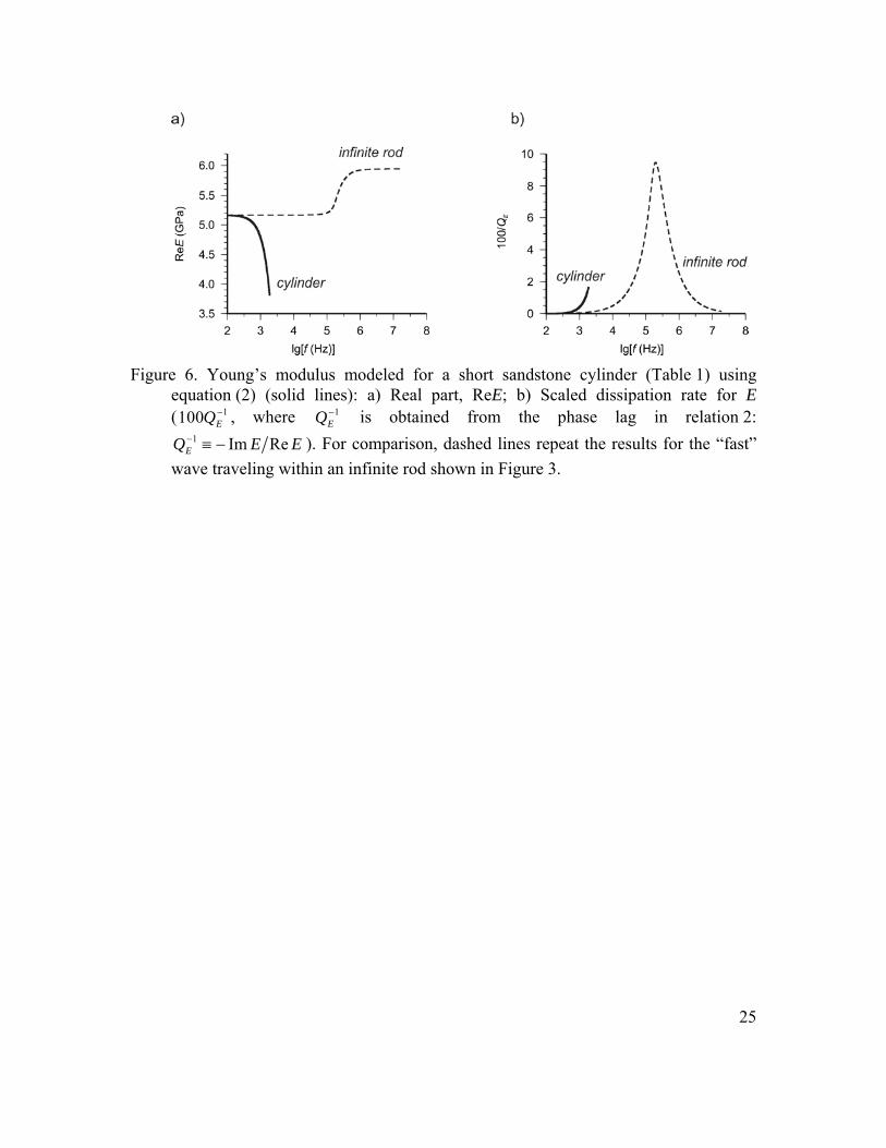
As stated in equation (2), the measured empirical (dynamic) Young’s modulus equals LE . This quantity is shown in Figure 6 for low frequencies according to

the approximation used in Appendix A. This modeling is performed for L = 11 cm and frequencies selected so that the fast-mode wavelengths exceed 8L, which is adequate for subresonant laboratory measurements. Since both fast and slow waves contribute in L and , the modulus E is intermediate between Efast and Eslow evaluated for the traveling waves in the preceding section (Figure 6).

Because the relative amplitudes of the fast and slow modes within the specimen vary with frequency, the relation between E, Efast and Eslow is complicated and depends on the frequency and sample length. There appears to exist no simple relation to empirically relate these quantities. Note that the decrease of ReE and QE with frequency (solid lines in Figure 6) occurs at ~1 kHz, which is 10–100 times lower than the dissipation peak for the infinite rod (dashed lines in the same Figure). This low-frequency rise in the frequency dependence of ReE and QE for the cylinder is principally caused by an increase in the contributions from the slow modes.

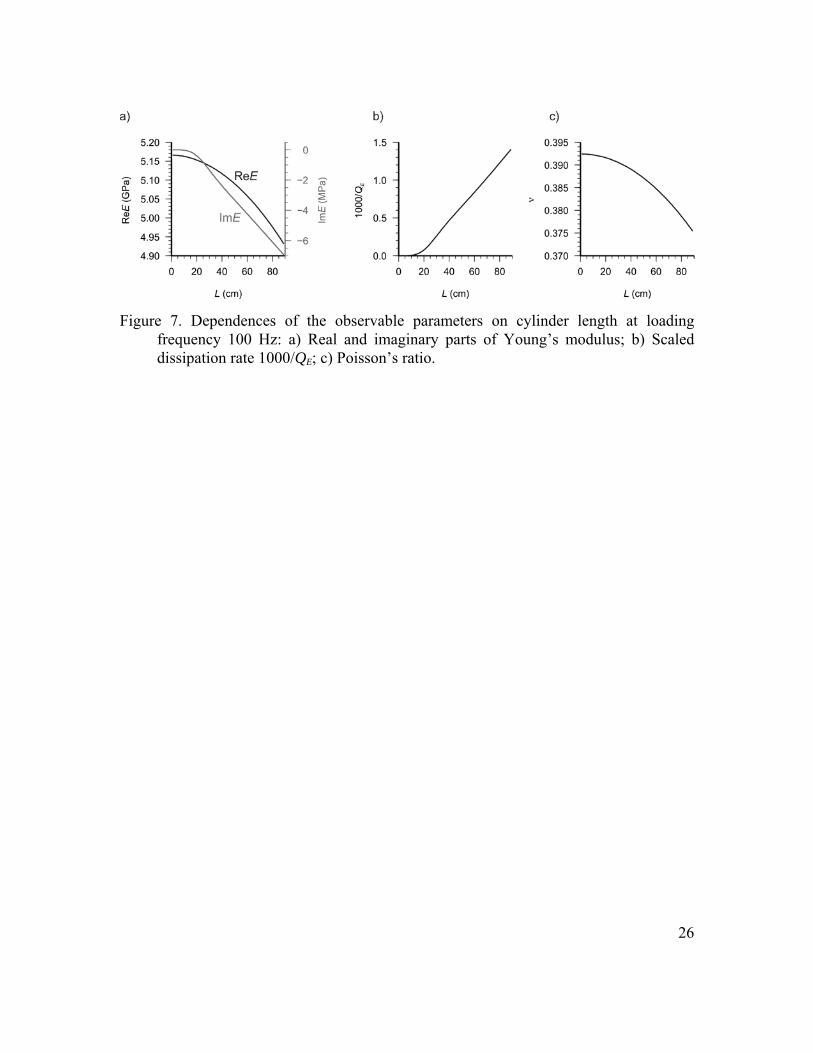
Because the wavelengths of slow waves are larger but comparable to the length of the cylinder L (Figure 5), the measured quantities vary with changing L. At a loading frequency of 100 Hz, such variations are illustrated in Figure 7 for L ranging from zero to two wavelengths of the slow P wave. The real part of the modulus, ReE, decreases with increasing L but is approximately constant and equal the “elastic” Young’s modulus for short cylinders with L < 10–20 cm (black line in Figure 7a). The Poisson’s ratio similarly decreases with L (Figure 7c).

Another notable result of this modeling shows that the imaginary part of the Young’s modulus, ImE, is near zero for L below 10–20 cm, above which it quickly increases in negative magnitude (gray line in Figure 7a). This leads to a very low 1

EQ

(strain-stress phase lag) for short cylinders, with a steep increase above L ≈ 20 cm (Figure 7b). The near-zero dissipation for short cylinders is easy to understand. Recall that the pore fluid flow is constrained by u2x = 0 (no fluid flows) at both boundaries.

14

When the boundaries become much closer together than the slow wave lengths, this constraint forces the values of u2x to be near zero within the whole specimen. As a result, the weak fluid flow u2x 0 leads to low internal friction and small strain-stress phase lags.

Discussion

The above results may disagree with the intuitive reading of the viscoelastic model which is often used to explain seismic attenuation experiments. Dynamic moduli can certainly be modeled and measured in a variety of environments by using either relations (1) or (2), and yet these quantities are not necessarily “moduli” in the sense of (visco)elastic relations (4)–(6). This difference may make it difficult to relate the dynamic moduli measured in the laboratory (typically the Young’s modulus for compressional deformation) to those describing seismic waves in the field (typically the P-wave modulus). The dynamic moduli for a traveling wave are also significantly different from those for a short rock cylinder (Figure 6).

For waves in fully saturated uniform sandstone in Figures 3 and 4, the violations of viscoelastic relations (4)–(6) are weak below about 10 kHz, and it might therefore appear that we should not be concerned about them in practical measurements. Nevertheless, note that relations (4)–(6) hold at these frequencies only inasmuch the rocks are approximately elastic (i.e., the moduli are constant). At all frequencies, the Q-1 measured from the stress/strain ratio (2) within a wave is about four times larger than the Q-1 inferred from the wave attenuation relation (1) (Figure 2b). The frequency dependences of the anelastic parts of the poroelastic and viscoelastic predictions are opposite (Figures 3b and 4b), and the differences between them are of the same order as the Q-1 (Figure 2b).

For the same deformation type, the frequency-dependent moduli measured in subresonant laboratory tests with small specimens (i.e., in a forced standing wave) are much weaker and have much stronger dissipation than in a traveling wave (Figure 6). The deviation from elasticity in a small specimen starts at much lower frequencies (~100-1000 Hz) than in a traveling wave and shows an opposite sense of variation with frequency (Figure 6a). These variations, and particularly the Q-1, strongly depend on the length of the cylindrical specimen (Figure 7b). The reason for all these effects is that the diffusive secondary wave penetrates the whole specimen, and the amount of this penetration varies with frequency and specimen size.

The dynamic bulk modulus, K, is a particularly delicate quantity, because it is extremely difficult to measure in field data. This modulus only exists within the viscoelastic model, and apparently the only direct observation of it comes from the radial free-oscillation mode 0S0 of the whole Earth (Knopoff, 1964). In laboratory studies, the bulk modulus is derived from the elastic-moduli relations such as (6). Since these relations appear to be limited for poroelastic materials, the significance of the dynamic K for them appears unclear.

15

The above observations show that the picture of mechanical behavior of a fluid-saturated porous rock may become quite complicated if based on the empirical dynamic moduli. The difficulty arises from commonly considering only the modulus for the primary (‘fast’) wave. If the moduli for the secondary modes are also included and reflections from the ends of the cylinder are taken into account, the moduli-based picture becomes consistent. Such a model was given by equations (19)–(21) in this paper.

However, attributing a modulus to every wave mode gives only a mathematical summary of the modal spectrum for a mechanical body. This spectrum is controlled by two factors: 1) properties of the material (equations of motion), and 2) the shape of the body and boundary conditions. Multiple dynamic moduli represent properties of the wave modes but not of the medium. For different body shapes, for example spherical saturation patches considered by White (1975) and Dutta and Odé (1979a), the dynamic-moduli spectrum should be different from the 1-D plane-wave modes considered here. As we are primarily interested in material properties, we need to deemphasize the boundary effects and emphasize the equations of motion (8), constitutive relation (9), and the matrix material properties (10). As noted by Geertsma and Smit (1961), these equations are not viscoelastic, which can be seen in the frictional term idu entering equation (8) outside

of the stress tensor and without the divergence operator required for the stress field (term

j ij σ ). The Darcy friction is a body force that cannot be incorporated in the viscoelastic

stress.

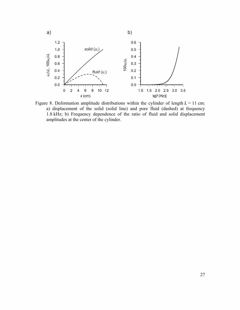
To further illustrate the difference of the pore-fluid friction from the strain-induced friction in the viscoelastic model, Figure 8a shows the distribution of the solid and fluid displacements within the cylinder at frequency 1.8 kHz. The distribution of fluid flow is non-uniform, even though the strain within the entire cylinder is practically constant. The distribution of u2 is also asymmetric, with a peak shifted toward the moving end of the cylinder. This asymmetry is due to the inertia of the pore fluid. If fluid saturation is non-uniform, this asymmetry could lead to different attenuation results depending on which end of the cylinder being loaded. For example, in the apparatus by Tisato and Madonna (2012), the cylindrical rock specimen is oriented vertically, and its saturation may be lower at the top because of the effect of gravity. Consequently, we might expect different values of attenuation when measured with the actuator placed at the bottom of the cylinder instead of its top, or with the whole device oriented horizontally. Such effects could apparently be easily tested experimentally. In addition, Figure 8a shows that fluid motion within the cylinder becomes significant at frequencies above about 100–300 Hz, which correspond to the increase of attenuation in Figure 6b.

The above observations are made for poroelasticity, for which a rigorous first-principle macroscopic theory is available (Biot, 1962; Bourbié et al., 1987). Qualitatively, similar observations could also be relevant to WIFF effects such as patchy saturations and squirt flows. With patchy saturation, the increase in velocity dispersion and attenuation occurs at lower frequencies, but the general mechanism of internal friction remains the same (fluid flow through heterogeneous rock matrix). The key feature of poroelasticity is the mutual friction between the two constituents of the

16

material (term idu in eq. (8)), which should likely be present in any model of rock

containing fluids. Also similarly to poroelasticity, WIFF media contain internal degrees of freedom (local fluid flows) and should therefore allow matrix parameterizations as in eqs. (10), support multiple wave modes (Dutta and Odé, 1979a) and consequently possess multiple P-wave moduli. Different geometries of saturation heterogeneity need to modeled specifically (e.g., White, 1975; Johnson, 2001; Rubino and Holliger, 2012; Kuteynikova, et al., 2014). However, it appears unlikely that the differences from viscoelasticity noted in the present study would disappear in the more complex WIFF cases.

Conclusions

The concept of viscoelastic modulus is useful for summarizing laboratory and field observations but it may be incomplete or complicated when representing the properties of fluid-saturated porous rock. The empirical dynamic moduli measured in various experiments represent combinations of the moduli for primary and secondary waves. These combinations vary with frequency, wave or oscillation types, and experiment geometry. Comparisons of the dynamic moduli modeled for traveling waves and subresonant oscillations of a sandstone cylinder show that at nonzero frequencies:

1) For waves, the dynamic moduli defined from phase velocities ( *2phaseM V )

and stress/strain ratios ( M ) are different. The amplitudes of the attenuation peaks differ by about four times for these moduli.

2) The dynamic moduli measured in short cylinders are lower than those in traveling waves in unbounded media. The attenuation (Q-1) in a sandstone cylinder is much higher and starts increasing at ~10–100 times lower frequencies than the poroelastic dissipation peaks in traveling waves.

3) At nonzero frequencies, the P-wave and Young’s moduli and Poisson’s ratios deviates from the usually assumed viscoelastic relations. For brine-saturated sandstone, the deviation becomes significant at frequencies above ~10 kHz.

4) For short cylindrical specimens (below 1 m at 100-Hz frequency), the measured modulus decreases and the attenuation strongly increases with the length of the cylinder. The dependence of Q-1on the length is nonlinear, with very low attenuation for cylinders shorter than about 20 cm.

Qualitatively, these observations likely apply to the more general cases of wave-induced flow (WIFF). To avoid the complexity of studying multiple dynamic moduli for all primary and secondary modes, first-principle approaches can be used to describe the wave-propagating media, compare laboratory and field observations, and make petrophysical conclusions.

17

Acknowledgements

Octave software (https://www.gnu.org/software/octave/) was used for calculations. Plots were produced using the Generic Mapping Tools (http://gmt.soest.hawaii.edu/).

References

Adam, L., M. Batzle, K. T. Lewallen, and K. van Wijk (2009). Seismic wave attenuation in carbonates: Journal of Geophysical Research, 114, B06208, doi: 10.1029/2008JB005890.

Batzle, M. L., G. Kumar, R. Hoffmann, L. Duranti, and L. Adam (2014). Seismic-frequency loss mechanisms: Direct observations, The Leading Edge, 33, 656-662.

Ben-Menahem, A., and S. J. Singh (1981). Seismic waves and sources, Springer-Verlag

Biot, M. A. (1962). Mechanics of deformation and acoustic propagation in porous media, J. Appl. Phys. 23, 1482–1498.

Bourbié, T., O. Coussy, and B. Zinsiger (1987). Acoustics of porous media, Editions TECHNIP, France, ISBN 2-7108-0516-2

Cooper, R. (2002). Seismic wave attenuation: Energy dissipation in viscoelastic crystalline solids, in: S.-I, Karato and H. R. Wenk (Eds.), Plastic deformation of minerals and rocks, Rev. Mineral Geochem., 51, 253–290.

Coulman, T., W. Deng, and I. Morozov (2013). Models of seismic attenuation measurements in the laboratory, Canadian J. Expl. Geoph, 38 (1), 51–67.

Dunn, K.-J. (1986). Acoustic attenuation in fluid-saturated porous cylinders at low frequencies, J. Acoust. Soc. Am., 79, 1709-1721.

Dutta, N. C., and H. Odé (1979a). Attenuation and dispersion of compressional waves in fluid-filled porous rocks with partial gas saturation (White model)–Part I: Biot theory, Geophysics, 44 (11), 1777–1788.

Dutta, N. C., and H. Odé (1979b). Attenuation and dispersion of compressional waves in fluid-filled porous rocks with partial gas saturation (White model)–Part II: Results, Geophysics, 44 (11), 1789–1805.

Geertsma, J., and D. C. Smit (1961). Some aspects of elastic wave propagation in fluid-saturated porous solids, Geophysics, 26 (2), 161–181.

Jackson, I., and M. S. Paterson (1993). A high-pressure, high-temperature apparatus for studies of seismic wave dispersion and attenuation, Pure Appl. Geoph. 141 (2/3/4), 445–466.

Johnson, D.L. (2001) Theory of frequency dependent acoustics in patchy-saturated porous media, J. Acoust. Soc. Am. 110 (2), 682–694

Knopoff, L. (1964). Q. Rev Geophys. 2(4), 625–660.

18

Kuteynikova, M., N. Tisato, R. Jänicke, and B. Quintal (2014). Numerical modelling and laboratory measurements of seismic attenuation in partially saturated rock, Geophysics, 79(2), L13-L20, doi: 10.1190/GEO2013-0020.1

Lakes, R. (2009). Viscoelastic materials, Cambridge, ISBN 978-0-521-88568-3.

Lakes R.S., and A. Wineman (2006). On Poisson’s ratio in linearly viscoelastic solids, J Elasticity 85, 45–63

Landau L. D., and E. M. Lifshitz (1986). Course of theoretical physics, volume 7 (3rd English edition): Theory of elasticity, Butterworth-Heinemann, ISBN 978-0-7506-2633-0

Lines, L., J. Wong, K. Innanen, F. Vasheghani, C. Sondergeld, S. Treitel, and T. Ulrych (2014). Research Note: Experimental measurements of Q-contrast reflections, Geophysical Prospecting 62, 190–195, doi: 10.1111/1365-2478.12081

Liu, H. P., D. L. Anderson, and H. Kanamori (1976). Velocity dispersion due to anelasticity: implications for seismology and mantle composition, Geophys. J. R. Astr. Soc., 47, 41–58.

Morozov, I. B. (2010). On the causes of frequency-dependent apparent seismological Q. Pure Appl. Geophys., 167, 1131–1146, doi 10.1007/s00024-010-0100-6.

Morozov I. B. (2011). Anelastic acoustic impedance and the correspondence principle. Geophys. Prosp., 50, 24-34, doi 10.1111/j.1365-2478.2010.00890.x

Müller, T., B. Gurevich, and M. Lebedev (2010). Seismic wave attenuation and dispersion resulting from wave-induced flow in porous rock – A review, Geophysics 75, 75A147 – 75A164.

Rubino, J. G., and K. Holliger (2012). Seismic attenuation and velocity dispersion in heterogeneous partially saturated porous rock: Geophysical Journal International, 188, 1088-1102, doi: 10.1111/j.1365-246X.2011.05291.x

Tisato N. and C. Madonna (2012). Attenuation at low seismic frequencies in partially saturated rocks: Measurements and description of a new apparatus, Journal of Applied Geophysics 86, 44-53.

Tschoegl, N.W., Knauss ,W., and Emri, I. (2002). Poisson’s ratio in linear viscoelasticity – a critical review, Mech Time-Depend. Mater., 6, 3–51

White, J. E. (1965), Seismic waves: Radiation, transmission, and attenuation: McGraw-Hill.

White, J. E. (1975). Computed seismic speeds and attenuation in rocks with partial gas saturation, Geophysics, 40 (2), 224–232.

19

Tables

Table 1. Physical parameters of brine-saturated sand used in the examples (after Dutta and Oté (1979)

Rock VP 1500 m/s P-wave velocity of dry matrix VS 1000 m/s S-wave velocity of dry matrix Ks 35 GPa Bulk modulus of solid grains s 2650 kg/m3 Density of solid grains 0.3 Porosity 9.86923310-13 (1 Darcy) Permeability a 1 Tortuosity

Brine Kfl 2.4 GPa Bulk modulus fl 1000 kg/m3 Density 110-3 Viscosity

20

Figures

Figure 1. Schematic experiments for measuring the Young’s moduli: a) Using a wave traveling in an infinite rod. One fast wave mode is used (arrow) and the modulus is defined by relation (1). b) Using constant-frequency loading of a small specimen in the laboratory. A superposition of four wave modes traveling in both directions is used (labeled arrows), and the modulus is defined by the stress-strain ratio (2).

21

Figure 2. Modeled dependences of the P-wave modulus on frequency for a wave in sandstone: a) real part; b) dissipation factor 1/Q for the primary mode. Solid lines correspond to the moduli defined from wave velocities (1), dashed lines show the stress/strain ratios (2). In plot a), the results for the slow wave are shown in gray.

22

Figure 3. Ratio E/M of the Young’s (E) and P-wave moduli (M) for the fast P wave in an infinite poroelastic rod: a) Re(E/M); b) Im(E/M). Solid lines are the exact values obtained by solving the poroelastic equations (8), and dashed lines are inferred by transformations of the moduli (5).

23

Figure 4. Frequency dependence of the Poisson’s ratio for a traveling wave in sandstone rod (Table 1): a) real part; b) imaginary part. Solid lines show the exact solution of equations (8), and dashed lines – solution inferred from viscoelastic moduli (the second equation (4)).

24

Figure 5. Fast- (solid lines) and slow-wave (dashed lines) wavelengths (black) and skin depths (gray) in an infinite rod or cylinder modeled in this paper (Table 1). Gray bar schematically shows the range of cylinder lengths L used in laboratory experiments for attenuation.

25

Figure 6. Young’s modulus modeled for a short sandstone cylinder (Table 1) using equation (2) (solid lines): a) Real part, ReE; b) Scaled dissipation rate for E ( 1100 EQ , where 1

EQ is obtained from the phase lag in relation 2: 1 Im ReEQ E E ). For comparison, dashed lines repeat the results for the “fast”

wave traveling within an infinite rod shown in Figure 3.

26

Figure 7. Dependences of the observable parameters on cylinder length at loading frequency 100 Hz: a) Real and imaginary parts of Young’s modulus; b) Scaled dissipation rate 1000/QE; c) Poisson’s ratio.

27

Figure 8. Deformation amplitude distributions within the cylinder of length L = 11 cm: a) displacement of the solid (solid line) and pore fluid (dashed) at frequency 1.8 kHz; b) Frequency dependence of the ratio of fluid and solid displacement amplitudes at the center of the cylinder.

28

Appendix A: Dynamic moduli for traveling waves

To utilize the matrix equations (8) and (9), it is convenient to define additional matrices relating the strains to the independent variables of the problem. Matrix computations are compact and can be readily implemented in engineering software such as Matlab or Octave.

Let us consider the boundary conditions related to evaluating the P-wave and Young’s moduli concurrently. In both the P-wave and infinite-rod problems, the axial displacements u1x(x,t) and u2x(x,t) can be taken as independent variables combined in a model vector:

1

2

x

x

u

u

q . (A1)

As shown in equations 17, the transverse deformation of the rod can be parameterized by the transverse strain yy(x,t) xx(x,t). Then, the strains and the three components of displacement for the rock and axial displacement of the filtration fluid can then be written as:

1

1

1

2

x

y

z

x

u

u

u

u

Uq U q and

1

1

1

1

1

xx

yy

zz

xy

xz

ΕUq , (A2)

where:

1 0

0 0

0 0

0 1

U , (A3)

and matrices U, and E depend on the conditions on the transverse boundary. For the P-wave case (zero transverse strain), these matrices equal:

0 0

0 0

0 0

0 0

U , and

1 0 0 0

0 0 0 0

0 0 0 0

0 1 2 0 0

0 0 1 2 0

Ε . (A4)

29

In this case, the second and third rows in these matrices can be dropped, as well as the corresponding columns in E and matrices and V below. For a rod with free transverse boundary (equations 17):

1 2

1 2

1 0

0 1

y y

z z

U , and 1 2

1 2

1 0 0 0

0 0

0 0

0 1 2 0 0

0 0 1 2 0

Ε . (A5)

Note that for attenuating harmonic waves, the spatial derivative operators can be replaced by sgnx i k i k , and the time derivatives by t i .

From E, a similar matrix for deviatoric strain Ε can be obtained by subtracting 1/3 of their sum from each of the first three rows in E. The dilatational strains can be combined in a 2-component vector and also written as a matrix product:

1

2

ΩUq , (A6)

where, for the P-wave case:

1 0 0 0

0 0 0 1

Ω , (A7)

and for the free transverse boundary case:

1 21 2 0 0 2

0 0 0 1

Ω . (A8)

The simplest approach to deriving the equations of motion for q(t,x) is to consider the functional forms of the potential and kinetic energies and the dissipation function on q and q (the overdot denotes the time derivative of q; Bourbié et al., 1987). With the strains given by equations (A2) and (A6), the elastic energy density is quadratic with respect to q (ibid):

1 1

2 2T T T

ij ijV Δ KΔ ε με q Λq , (A9)

where matrix K is given in relations 10, and matrix:

2T T T Λ U Ω KΩ Ε VΕ U (A10)

30

acts as the effective elastic modulus for the type of deformation considered, i.e., the coordinates (A1)–(A5). In this expression, matrix 1,1,1,2,2diagV is needed for

evaluating the tensor product Tij ijε ε as dot product of the vector (A2).

The kinetic energy is also quadratic with respect to u :

1

2Ti iT u ρu . (A11)

Taking into account the first equation A2, this energy can be expressed through q and q :

1 1 1

2 2 2T qΓq qΓ q q Γ q , (A12)

where matrices Γ , and Γ describe the kinematic coupling between the rock and pore fluid within the rod. For harmonic oscillations, the second and third terms in this expression are proportional to 3 and 4, respectively, and therefore we disregard them at low frequencies. The kinematic coupling matrix in the first term equals (ibid; compare to relations (10)):

0 0

0 0 0

0 0 0

0 0

f

T

f f

a

Γ U U . (A13)

The kinetic energy density increases towards the surface of the rod, as yu and zu linearly

increase with distance from the axis of the rod. However, the contributions from yu and

zu belong to the terms containing q (eqs. (A2) and (A12)), which are disregarded in the

low-frequency approximation.

Pore-fluid flow (Darcy) friction is described by the dissipation pseudo-potential that has a functional form similar to the kinetic energy above:

1 1

2 2T Ti iD u du qU ΘUq , (A14)

where:

31

0 0 0 0

0 0 0 0

0 0 0 0

0 0 0

Θ . (A15)

With the above quadratic expressions for all energies and D, and considering a harmonic wave attenuating in the positive direction of axis X (relation (13) in the text), the wave equation becomes (ibid):

22 Ti k i Γq U ΘUq Λq , (A16)

Note that the right-hand side of this equation represents a divergence of the elastic stress (surface force for an elementary volume), and the left-hand side contains the inertial and frictional body forces. This equation represents a generalized eigenvalue problem for vector q:

* ρ q Λq , (A17)

where the eigenvalue 2 2k i , and the matrix * can be viewed as “effective

complex density”:

* Ti

ρ Γ U ΘU . (A18)

Equation A17 represents an eigenvalue problem for , from which the complex phase velocity can be obtained as * 1V . For the P-wave case (matrix U in (A4)), the two

variables responsible for thickening of the rod in the directions Y and Z can be dropped, and then the 22 matrix = M represents the matrix P-wave modulus in equations (10): = , Θ d , and equations (A16) and (A18) reduce to equation (14) in the text (ibid).

The scalar P-wave or Young’s moduli are measured as ratios of the axial components of stress and strain in the respective experiments (equation (2) in the text). This ratio needs to be evaluated separately for the fast and slow modes of the P wave,

given by the corresponding eigenmode nq in (A17). For eigenmode n, the strain xx is

given by the first component of vector ( ) ( )

1 13n n ikxik e ΩUq ΕUq , where subscript

‘1’ denotes the first element of the corresponding vectors, and k is the complex wavenumber. The first term in this expression contains the xx-component of the dilatational strain, and the second is the deviatoric strain. The strain xx is (in principle) readily measurable. Regarding the stress, its measurement within the wave is more difficult. Hypothetically, let us assume that xx is measured by inserting a small

32

piezometer in a gap within the wave and ensuring that this insertion does not alter the wave pattern. Then, the axial stress measured by the piezometer is the surface stress:

( ) ( )

1 12n n ikx

xx ik e KΩUq ΕUq . (A19)

This value is affected by neither the Darcy friction nor inertia, because both of these are body forces. Consequently, the measured empirical scalar modulus equals:

( ) ( )

1 1( ) ( )

1 1

2

3

n n

xx n nM

KΩUq ΕUq

ΩUq ΕUq

. (A20)

As illustrated on an example of sandstone in the text (Figure 2), this modulus is frequency-dependent and differs from the modulus defined by using the phase velocity, 2

phaseM V .

For → 0, the effects of both inertia and friction d are negligible, and the fast

wave contains no fluid motion: (fast) 1,0Tq . As it can be readily verified, the modulus

Mxx in equation (A20) then equals the P-wave modulus 4 3f fM K for U and E

given in (A4), and Young’s modulus 12 1fE in (A5).

33

Appendix B: Transverse elastic stress in a poroelastic cylinder (equation (16))

Denoting the two nonzero components of the axially-symmetric strain for the body by 1xx and 1yy = 1zz and the relative strain of filtration fluid 2xx, the dilatational strain of the body becomes 1 1 12xx yy , and the transverse component of the deviatoric strain

1 1 1 1 13 3yy yy yy xx . From relation (9), the dilatational stress then equals:

11 1 1 2

2

2f xx yy xxp K M

K , (B1)

and the transverse deviatoric stress 1 1 12 3yy yy xx . By adding these stresses, we

obtain the total transverse stress 1 1yy yyp as a function of arbitrary 1xx, 1yy, and

2xx, given in equation (16).