Robustness in Hypervolume-basedMultiobjective Search

TIK Report 317

Johannes Bader johannes.bader@tik.ee.ethz.chComputer Engineering and Networks Laboratory, ETH Zurich, 8092 Zurich,Switzerland

Eckart Zitzler eckart.zitzler@tik.ee.ethz.chComputer Engineering and Networks Laboratory, ETH Zurich, 8092 Zurich,Switzerland

Abstract

The use of quality indicators within the search has become a popular approach in thefield of evolutionary multiobjective optimization. It relies on the concept to transformthe original multiobjective problem into a set problem that involves a single objectivefunction only, namely a quality indicator, reflecting the quality of a Pareto set approx-imation. Especially the hypervolume indicator has gained a lot of attention in thiscontext since it is the only set quality measure known that guarantees strict monotonic-ity. Accordingly, various hypervolume-based search algorithms for approximating thePareto set have been proposed, including sampling-based methods that circumventthe problem that the hypervolume is in general hard to compute.

Despite these advances, there are several open research issues in indicator-based mul-tiobjective search when considering real-world applications—the issue of robustnessis one of them. For instance with mechanical manufacturing processes, there existunavoidable inaccuracies that prevent a desired solution to be realized with perfectprecision; therefore, a solution in terms of a concrete decision vector is not associatedwith just one one fixed vector of objective values, but rather with a range of objectivevalues that reflect the variance when slightly changing the decision variables. As aconsequence, the optimization model needs to account for such uncertainties and thesearch method is required to explicitly integrate robustness considerations.

While in single-objective optimization, there are various studies dealing with the ro-bustness issue, there are considerably fewer in the multiobjective optimization litera-ture and none in the context of hypervolume-based multiobjective search. This studyis set in the latter context and addresses the question of how to incorporate robustnesswhen using the hypervolume indicator within an evolutionary algorithm. To this end,three common robustness concepts are translated to and tested for hypervolume-basedsearch on the one hand, and an extension of the hypervolume indicator is proposed onthe other hand that not only unifies those three concepts, but also enables to realizemuch more general trade-offs between objective values and robustness of a solution.Finally, the approaches are compared on two test problem suites as well as on a newlyproposed real-world bridge construction problem.

Keywords

robustness, hypervolume indicator, multiobjective optimization, multiobjective evolu-tionary algorithm, Monte Carlo sampling, truss bridge problem

1 Introduction

In multiobjective optimization, using the hypervolume indicator to find Pareto-optimalsolutions has become popular in recent years. The reason for the popularity of this mea-sure is its strict monotonicity with respect to Pareto dominance (Zitzler et al., 2003). Asa consequence hypervolume-based algorithms can be designed to guarantee a theoret-ical convergence behavior (Brockhoff et al., 2008; Zitzler et al., 2009). Existing multi-objective techniques that combine Pareto dominance with a specific diversity measure,e.g., (Deb et al., 2000; Zitzler et al., 2001), often fail in this regard on problems involv-ing a larger number (e.g., larger than four) of objectives due to cyclic behavior (Wagneret al., 2007; Zitzler et al., 2008). Although the basic hypervolume-based search approachhas been investigated and extended in different directions, e.g., with regard to the biasof the indicator (Brockhoff et al., 2008; Auger et al., 2009b; Friedrich et al., 2009), to theincorporation of user preferences (Zitzler et al., 2007; Auger et al., 2009a), and to the hy-pervolume calculation resp. estimation (While et al., 2005; Beume and Rudolph, 2006;Fonseca et al., 2006; Bader and Zitzler, 2008), the issue of robustness has not been ad-dressed so far to the best of our knowledge. A few studies have used the hypervolumeas a measure of robustness though: Ge et al. (2005) have used the indicator to assess thesensitivity of design regions according to the robust design of Taguchi (1986); a similarconcept by Beer and Liebscher (2008) uses the hypervolume indicator to measure therange of possible decision variables that lead to the desired range of objective values;a study by Hamann et al. (2007) applied the hypervolume indicator in the context ofsensitivity analysis. However, none of these papers deals with integrating robustnessinto hypervolume-based multiobjective search.

Robustness becomes an important issue when tackling real-world applications.Solutions to engineering problems, for instance, can usually not be manufactured arbi-trarily accurate such that the implemented solution and its objective values differ fromthe original specification, up to the point where they become infeasible. Designs whichare seriously affected by perturbations of any kind might no longer be acceptable to adecision maker from a practical point of view—despite the promising theoretical result.The corresponding uncertainty due to production variations, which reflects the secondcategory of uncertainty defined in Beyer and Sendhoff (2007), needs to be taken intoaccount within both optimization model and algorithm in order to find robust solu-tions that are relatively insensitive to perturbations. Ideally, there exist Pareto-optimaldesigns whose characteristics fluctuate within an acceptable range. Yet, for the mostpart robustness and quality (objective values) are irreconcilable goals, and one has tomake concessions to quality in order to achieve an acceptable robustness level.

Many studies have been devoted to robustness in the context of single-objectiveoptimization, e.g., (Taguchi, 1986; Jin and Branke, 2005; Beyer and Sendhoff, 2007).However, most of these approaches are not applicable to multiobjective optimization.The first approaches (Kunjur and Krishnamurty, 1997; Tsui, 1999) to consider robust-ness in combination with multiple objectives are based on the design of experimentapproach (DOE) by Taguchi (1986); however, they aggregate the individual objectivefunctions such that the optimization itself is no longer of multiobjective nature. Onlyfew studies genuinely tackle robustness in multiobjective optimization: one approach

2

by Teich (2001) is to define a probabilistic dominance relation that reflects the underly-ing noise; a similar concept by Hughes (2001) ranks individuals based on the objectivevalues and the associated uncertainty; Deb and Gupta (2006, 2005) considered robust-ness by either adding an additional constraint or by optimizing according to a fitnessaveraged over perturbations. The following classification categorizes most existing ro-bustness approaches in the evolutionary computing literature:

A — Replacing the objective value: Among the widest-spread approaches to accountfor noise is to replace the objective values by a measure or statistical value reflect-ing the uncertainty. Parkinson et al. (1993) for instance optimize the worst case.The same approach, referred to as “min max”, is also employed in other studies,e.g., in (Kouvelis and Yu, 1997; Soares et al., 2009a,b) . Other studies apply an aver-aging approach where the mean of the objective function is used as the optimiza-tion criterion (Tsutsui and Ghosh, 1997; Jurgen Branke, 1998; Branke and Schmidt,2003). In Mulvey et al. (1995) the objective values and a robustness measure areaggregated into a single value that servers as the optimization criterion.

B — Using one or more additional objectives: Many studies try to assess the robust-ness of solutions x by a measure r(x), e.g., by taking the norm of the varianceof the objective values (Jin and Sendhoff, 2003) or the maximum deviation fromf (x) (Deb and Gupta, 2006). This robustness measure is then treated as an addi-tional objective (Jin and Sendhoff, 2003; Egorov et al., 2002; Li et al., 2005). A studyby Burke et al. (2009) fixes a particular solution (a fleet assignment of an airlinescheduling problem), and only optimizes the robustness of solutions (the schedulereliability and feasibility).

C — Using at least one additional constraint: A third possibility is to restrict thesearch to solutions fulfilling a predefined robustness constraint, again with respectto a robustness measures r(x) (Gunawan and Azarm, 2004, 2005; Deb and Gupta,2005, 2006).

Combinations of A and B are also used; Das (2000) for example considers the expectedfitness along with the objective values f (x), while Chen et al. (1996) optimize the meanand variance of f (x).

Given these considerations, we investigate in the remainder of this paper howrobustness can be integrated in hypervolume-based multiobjective search. First, weaddress the question of how the three existing approaches A, B, and C mentioned abovecan be translated to a concept for the hypervolume indicator. Second, we introduce anovel approach that represents a generalization of the hypervolume indicator unifyingthe three approaches, and third we propose different search algorithms implementingthe various ideas. An empirical comparison on different test problems and a real-worldproblem provides valuable insights regarding advantages and disadvantages of thepresented approaches.

2 Background

2.1 Hypervolume-based Multiobjective Search

In the following, we consider a multiobjective objective optimization problem f : X →Z where X ⊆ Rn denotes the decision space and n denotes the number of decisionvariables. The decision space is mapped to the objective space Z ⊆ Rd by d objectivefunctions ( f1(x), . . . , fd(x)) = f (x); without loss of generality, all objectives are to be

3

minimized. Optimization is performed according to a preference relation ≼ on X. Theminimal elements of the ordered set (X,≼) constitute the optimal solutions formingthe Pareto set, whose image under f is called Pareto front.

The weak Pareto dominance forms an important preference relation ≼par on solu-tions, defined as x ≼par y :⇔ ∀i ∈ 1, . . . , n : fi(a) ≤ fi(b). In the following, weakPareto dominance ≼par is used as the standard preference on solutions, however, otherdefinitions, especially in the presence of uncertainty, are meaningful. In Sec. 3, we willpropose different relations which rank solutions a ∈ X not only based on the objec-tive values f (a), but also on a robustness measure r(a). All relations introduced so farinduce pre-orders and we use the usual definition for the corresponding strict orders(Harzheim, 2005); for example, Pareto dominance ≺par on two solutions a, b ∈ X isgiven by a ≺par b⇔ a ≼par b ∧ b ≼par a.

The above definitions on single solutions can be transferred to an equivalent onsets (Zitzler et al., 2009) where the search space Ψ = P(X) consists of all possible setsof solutions A ⊆ X, and the objective space Ω = P(Z) is formed by all sets U ⊆ Z ofobjective vectors 1. The set equivalent F : Ψ → Ω of the objective function maps a setof solutions to their objective values, i.e., X 7→ y | ∃x ∈ X, f (x) = y. The preferencerelation ≼ on solutions is extended to a set preference 4 on sets A, B in the followingcanonical way:

A 4 B :⇔ ∀b ∈ B ∃a ∈ A : a ≼ b (1)

where again the relation 0 on the objective space Ω is given by the isomorphic mappingof (Ψ,4) to (Ω,0) given by the objective function f . Due to practical limitations, thesearch space is usually restricted to elements not exceeding a fixed number of elementsα, i.e., Ψ≤α = A ∈ Ψ | |A| ≤ α where the relation 4≤α on Ψ≤α corresponds to therestriction of 4 to Ψ≤α, i.e., 4≤α:=4 Ψ≤α. Given such a relation on sets optimizationalgorithms strive to find (one of) the minimal elements of Ψ≤α for 4 Ψ≤α).

An important question in the context of optimizing sets is how to refine the Paretodominance 4par for the large number of cases where neither A 4par B nor B 4par Aholds, and therefore additional preference information is needed. Indicator functionsrepresent one possibility to obtain a total relation on sets. They assign each set A ∈ Ψ avalue representing its quality. Given this value, the relation ≼I on two sets A, B ∈ Ψ isdefined as A ≼I B :⇔ I(A) ≥ I(B). The hypervolume indicator is one popular choiceof indicator that has received more and more attention in recent years. It measures the(hyper-)volume of dominated portion of the objective space:

Definition 2.1. Let A ∈ Ψ denote a set of solutions and let r represents a reference point2, letw : Rk → R>0 denote a strictly positive weight function integrable on any bounded set. Thenthe hypervolume indicator for A is given as

IwH(A, R) =

(∞,...,∞)∫(−∞,...,−∞)

αA(z)w(z)dz with αA(z) =

1 A 0 z0 otherwise

(2)

1In fact, A and U in their most general form are multisets where duplicates of the same solution andobjective vector respectively are allowed. To avoid unwieldy notations, in this paper we stick to proper sets;the concepts, however, can be extended to multisets as well.

2In the most general definition of the hypervolume indicator, a reference set R is used instead of a singlereference point r. Without loss of generality, throughout this study we consider only a single reference pointr.

4

with αA(z) = 1H(A,R)(z) where

H(A, R) = z | ∃a ∈ A ∃r ∈ R : f (a) 6 z 6 r (3)

and 1H(A,r)(z) being the characteristic function of H(A, r) that equals 1 iff z ∈ H(A, r) and 0otherwise.

The reason for the popularity of the hypervolume indicator is that it is up to nowthe only indicator that is a refinement of the Pareto dominance, i.e., whenever for twosets A, B ∈ Ψ, A ≺par B holds, then Iw

H(A, R) > IwH(B, R), see (Zitzler et al., 2009). As a

consequence of this property, an improvement of any solution of set A will increase theindicator value, and the Pareto set A∗ achieves the maximum possible hypervolumevalue. For this reasons, many modern algorithms use the hypervolume indicator asunderlying (set-)preference for search (Igel et al., 2007; Emmerich et al., 2005; Fleischer,2003; Knowles et al., 2006; Zitzler et al., 2007; Bader and Zitzler, 2009).

Although also useful for mating selection, the main field of application of the hy-pervolume indicator is environmental selection. The aim thereby is to select from apopulation of solutions a subset of predefined size, which will constitute the popula-tion of the next generation. Normally, hypervolume-based algorithms perform envi-ronmental selection by the following two consecutive steps:

1. At first, all solutions of the original population are divided into fronts by non-dominated sorting (Goldberg, 1989; Srinivas and Deb, 1994); while the aforemen-tioned algorithms use Pareto-dominance as underlying dominance relation, inprinciple, however, also other relations can be used as will be demonstrated inSec. 3. Following the non-dominated sorting the fronts are, starting with the bestfront, inserted into the new population as a whole as long as the number of solu-tions in the new population does not exceed the predefined population size.

2. The first front A which can no longer be inserted into the new population is there-after truncated to the number of places to be filled. To this end, one after an-other the solution xw is removed which causes the smallest loss in hypervolumeIwH(A, R)− Iw

H(A\xw, R). After reach removal, the hypervolume losses are recal-culated. At the end, the truncated front is inserted in the new population whichconcludes environmental selection.

2.2 Robustness

Robustness of a solution informally means, that the objective values scatter onlyslightly under real conditions. These deviations, referred to as uncertainty, are oftennot considered in multiobjective optimization. This section shows one possibility toextend the optimization model proposed above by the consideration of uncertainty. Assource of uncertainty, noise directly affecting the decision variable x is considered. Thisresults in a random decision variable Xp, which is evaluated by the objective functioninstead of x. As distribution of Xp, this paper considers a uniform distribution:

Bδ(x) := [x1 − δ, x1 + δ]× . . .× [xn − δ, xn + δ] . (4)

The distribution according to Eq. 4 stems from the common specification of fabricationtolerances. Of course, other probability distributions for Xp are conceivable as well; ofparticular importance is the Gaussian normal distribution, as it can be used to describe

5

many distributions observed in nature. Although not shown in this paper, the proposedalgorithms work with other uncertainties just as well.

Given the uncertainty Xp, the following definition of Deb and Gupta (2005) can beused to measure the robustness of x:

r(x) =∥ f w(Xp)− f (x)∥

f (x)(5)

where f (x) denotes the objective values of the unperturbed solution, and f w(Xp) de-notes the objective-wise worst case of all objective values of the perturbed decisionvariables Xp:

f w(Xp) =(

maxXp

f1(Xp), . . . , maxXp

fd(Xp) (6)

From the multi-dimensional interval Bδ, the robustness measure r(x) may be deter-mined analytically (see Gunawan and Azarm (2005)). If this is not possible, for instancebecause knowledge of the objective function is unavailable, random samples are gener-ated within Bδ(x) and evaluated to obtain an estimate of the robustness measure r(x).

3 Concepts for Robustness Integration

As already mentioned in the introduction, existing robustness integrating approachescan roughly be classified into three basic categories: (i) modifying the objective func-tions, (ii) using an additional objective, and (iii) using an additional constraint. Totranslate these approaches to hypervolume-based search, one or multiple of the threemain components of hypervolume-based set preference need to be changed:

1. the preference relation is modified to consider robustness—this influences the non-dominated sorting.

2. The objective values are modified before the hypervolume is calculated.3. The definition of the hypervolume indicator itself is changed.

Depending on how the decision maker accounts for robustness, the preference re-lation changes to ≼rob. Note, that the relation≼rob does not need to be a subset of≼; infact, the relation can even get reversed. For example, provided solution x is preferredover y given only the objectives x ≼ y, but considering robustness y ≼rob x holds, forinstance because y has a sufficient robustness level but x does not.

The most simple choice of dominance relation is ≼rob ≡ ≼par, that is to not con-sider robustness. This concept is used as reference in the experimental comparison inSec. 5. Depending on the robustness of the Pareto set, optimal solutions according to≼par may or may not coincide with optimal solutions according to relations ≼rob thatconsider robustness in some way.

In the following, other preference relations, corresponding to the approaches A,B,and C on page 3, are shown. All resulting relations ≼rob thereby are not total. There-fore, to refine the relation, is is proposed to apply the general hypervolume-based pro-cedure: first, solutions are ranked into fronts by nondominated sorting according toSec. 2.1; after having partitioned the solutions, the normal hypervolume is applied onthe objective values alone or in conjunction with the robustness measure (which caseapplies is mentioned when explaining the respective algorithm) to obtain a preferenceon the solutions.

6

a

d

b

c

e

fg

h

ij

12

34

minimi-zation

(a) modifying the objectives

a

d

b

c

ef

g

ij

21

h

(b) additional objective

12

3

5

67

84

a

d

b

c

ef

gh

ij

(c) additional constraint

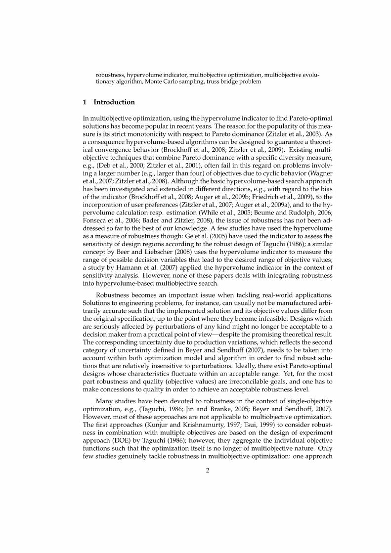
Figure 1: Partitioning into fronts of ten solutions: a (robustness r(a) = 2), b (2), c (1.4),d (1.1), e (2), f (1.2), g (1.9), h (.5), i (.9), and j (.1) for the three approaches presented inSec. 3. The solid dots represents robust solutions at the considered level of η = 1 whilethe unfilled dots represent non-robust solutions.

First, in Sec. 3.1, 3.2, and 3.3, we investigate how the existing concepts can be trans-formed to and used in hypervolume-based search. Then, in Sec. 3.4, these three con-cepts are unified into a novel generalized hypervolume indicator that also enables torealize other trade-offs between robustness and quality of solutions.

3.1 Modifying the Objective Functions

The first concept to incorporate robustness replaces the objective values f (x) =( f1(x), . . . , fd(x)) by an evaluated version over all perturbations f p(Xp) =

( f p1 (Xp), . . . , f p

d (Xp)), see Fig. 1(a). For example, the studies by Tsutsui and Ghosh(1997), Jurgen Branke (1998), and Branke and Schmidt (2003) all employ the mean overthe perturbations, i.e.,

f pi (Xp) =

∫xp

fi(xp)pXp(xp)dx (7)

where pXp(xp) denotes the probability density function of the perturbed decision vari-able Xp given x. Taking the mean will smoothen the objective space, such that f p

is worse in regions where the objective values are heavily affected by perturbations;while, contrariwise, in regions where the objective values stay almost the same withinthe considered neighborhood, the value f p differs only slightly. Aside from the alteredobjective value, the search problem stays the same. The regular hypervolume indicatorin particular can be applied to optimize the problem. The dominance relation implicitlychanges to ≼rob=≼repl with x ≼repl y :⇔ f p(x) 6 f p(y).

3.2 Additional Objective

Since the problems dealt with are already multiobjective by nature, a straightforwardway to also account for the robustness r(x) is to treat the measure as an additionalobjective (Jin and Sendhoff, 2003; Li et al., 2005; Guimaraes et al., 2006). As for theprevious approach, this affects the preference relation and thereby non-dominatedsorting, but also the calculating of the hypervolume. The objective function becomesf ao = ( f1, . . . , fd, r); the corresponding preference relation ≼oa is accordingly

x ≼ao y :⇔ x ≼par y ∧ r(x) ≤ r(y) . (8)

7

Considering robustness as an ordinary objective value has three advantages: first, apartfrom increasing the dimensionality by one, the problem does not change and existingmultiobjective approaches can be used. Second, different degrees of robustness arepromoted, and third, no robustness level has to be chosen in advance which wouldentail the risk of the chosen level being infeasible, or that the robustness level could bemuch improved with barely compromising the objective values of solutions. One dis-advantage of this approach is to not focus on a specific robustness level and potentiallyfinding many solutions whose robustness is too bad to be useful or whose objectivevalues are strongly degraded to achieve an unnecessary large degree of robustness. Afurther complication is the increase in non-dominated solutions resulting from consid-ering an additional objective, i.e., the expressiveness of the relation is smaller than theone of the previously stated relation≼repl and the relation proposed in the next section.

Fig. 1(b) shows the partitioning according to ≼ao. Due to the different robustnessvalues, many solutions which are dominated according to objective values only—thatis according to ≼par—become incomparable and only two solutions e and g remaindominated.

3.3 Additional Robustness Constraint

The third approach to embrace the robustness of a solution is to convert robustnessinto a constraint (Fonseca and Fleming, 1998; Gunawan and Azarm, 2005; Deb andGupta, 2005), which is then considered by adjusting the preference relation affectingnon-dominated sorting. We here use a slight modification of the definition of Deb andGupta (2005) by adding the additional refinement of applying weak Pareto dominanceif two non-robust solutions have the same robustness value. Given the objective func-tion f (x) and robustness measure r(x), an optimal robust solution then is

Definition 3.1 (optimal solution under a robustness constraint). A solution x∗ ∈ X withr(x∗) and f (x∗) denoting its robustness and objective value respectively, both of which are tobe minimized, is optimal with respect to the robustness constraint η, if it fulfills x∗ ∈ x ∈X | ∀y ∈ X : x ≼con y where

x ≼con y :⇔r(x) ≤ η ∧ r(x) > η ∨x ≼par y ∧ (r(x) ≤ η ∧ r(y) ≤ η ∨ r(x) = r(y)) ∨r(x) < r(y) ∧ r(x) > η ∧ r(y) > η

(9)

denotes the preference relation for the constrained approach under the robustness constraint η.

This definition for single solutions can be extended to sets according to the follow-ing definition:

Definition 3.2 (optimal set under a robustness constraint). A set A∗ ∈ Ψ with |A∗| ≤ αis optimal with respect to the robustness constraint η, if it fulfills

A∗ ∈ A ∈ Ψ | ∀B ∈ Ψ with |B| ≤ α : A 4con B (10)

where 4con denotes the extension of the relation ≼con (Eq. 9) to sets according to Eq. 1.

In the following, a solution x whose robustness r(x) does not exceed the constraint,i.e., r(x) ≤ η, is referred to as robust and to all other solutions as non-robust (Deb et al.,2002a).

8

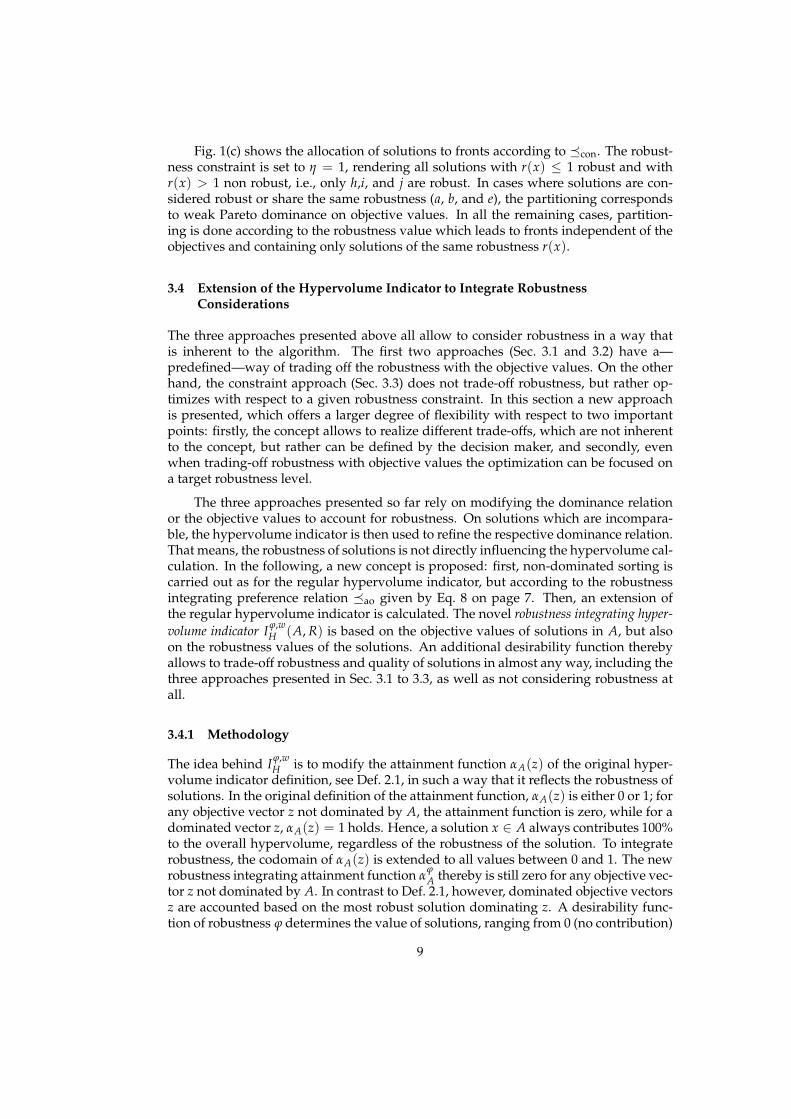
Fig. 1(c) shows the allocation of solutions to fronts according to ≼con. The robust-ness constraint is set to η = 1, rendering all solutions with r(x) ≤ 1 robust and withr(x) > 1 non robust, i.e., only h,i, and j are robust. In cases where solutions are con-sidered robust or share the same robustness (a, b, and e), the partitioning correspondsto weak Pareto dominance on objective values. In all the remaining cases, partition-ing is done according to the robustness value which leads to fronts independent of theobjectives and containing only solutions of the same robustness r(x).

3.4 Extension of the Hypervolume Indicator to Integrate RobustnessConsiderations

The three approaches presented above all allow to consider robustness in a way thatis inherent to the algorithm. The first two approaches (Sec. 3.1 and 3.2) have a—predefined—way of trading off the robustness with the objective values. On the otherhand, the constraint approach (Sec. 3.3) does not trade-off robustness, but rather op-timizes with respect to a given robustness constraint. In this section a new approachis presented, which offers a larger degree of flexibility with respect to two importantpoints: firstly, the concept allows to realize different trade-offs, which are not inherentto the concept, but rather can be defined by the decision maker, and secondly, evenwhen trading-off robustness with objective values the optimization can be focused ona target robustness level.

The three approaches presented so far rely on modifying the dominance relationor the objective values to account for robustness. On solutions which are incompara-ble, the hypervolume indicator is then used to refine the respective dominance relation.That means, the robustness of solutions is not directly influencing the hypervolume cal-culation. In the following, a new concept is proposed: first, non-dominated sorting iscarried out as for the regular hypervolume indicator, but according to the robustnessintegrating preference relation ≼ao given by Eq. 8 on page 7. Then, an extension ofthe regular hypervolume indicator is calculated. The novel robustness integrating hyper-volume indicator Iφ,w

H (A, R) is based on the objective values of solutions in A, but alsoon the robustness values of the solutions. An additional desirability function therebyallows to trade-off robustness and quality of solutions in almost any way, including thethree approaches presented in Sec. 3.1 to 3.3, as well as not considering robustness atall.

3.4.1 Methodology

The idea behind Iφ,wH is to modify the attainment function αA(z) of the original hyper-

volume indicator definition, see Def. 2.1, in such a way that it reflects the robustness ofsolutions. In the original definition of the attainment function, αA(z) is either 0 or 1; forany objective vector z not dominated by A, the attainment function is zero, while for adominated vector z, αA(z) = 1 holds. Hence, a solution x ∈ A always contributes 100%to the overall hypervolume, regardless of the robustness of the solution. To integraterobustness, the codomain of αA(z) is extended to all values between 0 and 1. The newrobustness integrating attainment function α

φA thereby is still zero for any objective vec-

tor z not dominated by A. In contrast to Def. 2.1, however, dominated objective vectorsz are accounted based on the most robust solution dominating z. A desirability func-tion of robustness φ determines the value of solutions, ranging from 0 (no contribution)

9

to 1 (maximum influence)3.Definition 3.3 (Desirability function of robustness). Given a solution x ∈ A with robust-ness r(x) ∈ R≥0, the desirability function φ : R≥0 → [0, 1] assesses the desirability of arobustness level. A solution x with φ(r(x)) = 0 thereby represents a solution of no avail dueto insufficient robustness. A solution y with φ(r(y)) = 1, on the other hand, is of maximumuse, and further improving the robustness would not increase the value of the solution.

Provided a function φ, the attainment function can be extended in the followingway to integrate robustness:

Definition 3.4 (Robustness integrating attainment function αφA). Given a set of solutions

A ∈ Ψ, the robustness integrating attainment function αφA : Z → [0, 1] for an objective vector

z ∈ Z, and a desirability function φ : r(x) 7→ [0, 1] is

αφA(z) :=

φ(

minx∈A, f (x)6z

r(x))

if A 0 z

0 otherwise(11)

Hence, the attainment function of z correspond to the desirability of the most robust solutiondominating z; and is 0 if no solution dominates z.

Finally, the robustness integrating hypervolume indicator corresponds to the es-tablished definition except for the modified attainment function according to Def. 3.4:Definition 3.5 (robustness integrating hypervolume indicator). The robustness integrat-ing hypervolume indicator Iφ,w

H : Ψ → R≥0 with reference set R, weight distribution functionw(z), and desirability function φ is given by

Iφ,wH (A) :=

∫Rd

αφA(z)w(z)dz (12)

where A ∈ Ψ is a set of decision vectors.

In the following, Iφ,wH is used to refer to the robustness integrating hypervolume

indicator, not excluding an additional weight distribution function to also incorporateuser preference. The desirability function φ not only serves to extend the hypervolumeindicator, but implies a robustness integrating preference relation:Definition 3.6. Let x, y ∈ X be two solutions with robustness r(x) and r(y) respectively.Furthermore, let φ be a desirability function φ : r(x) 7→ φ(r(x)). Then x weakly dominates ywith respect to φ, denoted x ≼φ y, iff x ≼par y and φ(r(x)) ≥ φ(r(y)) holds.

Since a solution x can be in relation ≼φ to y only if x ≼par y holds, ≼φ is a subre-lation of ≼par, and generally increases the number of incomparable solutions. In orderthat ≼φ is a reasonable relation with respect to Pareto dominance and robustness φ hasto be monotonically decreasing as stated in the following Theorem:Theorem 3.7. As long as φ is a (not necessarily strictly) monotonically decreasing function,and smaller robustness values are considered better, the corresponding robustness integratinghypervolume indicator given in Def. 3.5 (a) induces a refinement of the extension of ≼φ to sets,and (b) is sensitive to any improvement of non dominated solutions x with φ(r(x)) > 0 interms of objective value or the desirability of its robustness.

3The definition of desirabilty function used in this study is compliant with the definition known fromstatistical theory, cf. Abraham (1998).

10

x

(a) original set A

'x'x x

(b) objective value of x improved

''x( ( )) ( ( ))φ r x φ r x′′ >

(c) robustness of x improved

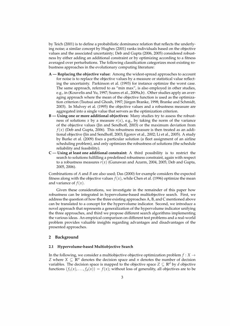
Figure 2: The robustness integrating hypervolume indicator is sensitive to improve-ments of objective values (b) as well as to increased robustness desirability (c).

Proof. Part 1: the robustness integrating hypervolume is compliant with the exten-sion of ≼φ to sets. Let A, B ∈ Ψ denote two sets with A ≼rob B. More specifi-cally this means, for all y ∈ B ∃x ∈ A such that x ≼par y and r(x) ≤ r(y). Nowlet y′B(z) := arg miny∈B, f (y)6z r(y). Then ∃x′A(z) ∈ A with x′A(z) ≼rob y′B(z). Thisleads to f (x′A(z)) 6 f (y′B(z)) 6 z and r(x′A) ≤ r(y′B). The latter boils down toφ(r(x′A)) ≥ φ(r(y′B)), hence α

φA(z) ≥ α

φB(z) for all z ∈ Z, and Iφ,w

H (A) ≥ Iφ,wH (B).

Part 2: the Def. 3.5 is sensitive to improvements of objective value and desirabil-ity. Let x ∈ A denote the solution which is improved, see Fig. 2(a). First, consider thecase where in a second set A′, x is replaced by x′ with r(x′) = r(x) and x′ ≺par x.Then there exists a set of objective vectors W which is dominated by f (x′) but not byf (x). Because of φ(r(x)) > 0, the gained space W increases the overall hypervolume,see Fig. 2(b). Second, if x is replaced by x′′ with the same objective value but a higherdesirability of robustness, φ(r(x′′)) > φ(r(x)), the space solely dominated by x′′ has alarger contribution due to the larger attainment value in this area, and again the hyper-volume indicator increases, see Fig. 2(c).

Note that choices of φ are not excluded for which the attainment function αφA(z)

can become 0 even if a solution x ∈ A dominates the respective objective vector z—namely if all solution dominating z are considered infeasible due to their bad robust-ness. Provided that φ is chosen monotonically decreasing, many different choices ofdesirability are possible. Here, the following class of functions is proposed, tailoredto the task of realizing the approaches presented above. Besides the robustness value,the function takes the constraint η introduced in Sec. 3.3 as an additional argument. Aparameter θ defines the shape of the function and its properties:

φθ(r(x), η) =

(

r(x)rmax− 1

)θ + (1 + θ)H1(η − r(x)) θ ≤ 0

exp(

3 · r(x)−ηη log(1−θ)

)0 < θ < 1, r(x) > η

1 otherwise

(13)

where H1(x) denotes the Heaviside function4, and rmax denotes an upper bound of therobustness measure. The factor 3 in the exponent is chosen arbitrarily, and only servesthe purpose of producing a nicely shaped function. By changing the shape parameter

4 H1(x) =

0 x < 01 x ≥ 0

11

−10

1

0

−1

0

1

-.5

.5

θ

( )r x ηη−

( )( ),θφ r x η

maxr ηη−

1

23

45

1

0-1 0 ( ) /maxr η η−

1

2

3

4

5

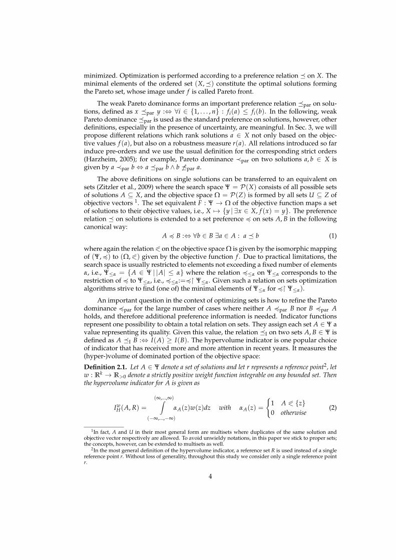
Figure 3: Desirability function φθ(r(x), η) according to Eq. 13. By changing the shapeparameter θ, different shapes of φ can be realized as shown in the cross-sectional plotsÀ to Ä. The robustness measure r(x) has been normalized to η, such that only solutionswith r(x) ≤ 0 are classified robust.

θ, different characteristics of φ can be realized that lead to different ways of trading offrobustness versus objective value, see Fig. 3:

À θ = 1: For this choice, φ1(r(x), η) ≡ 1. This means the robustness of solutions is notconsidered at all.

Á 0 < θ < 1: All solutions with r(x) ≤ η are maximally desirable in terms of robust-ness. For non robust solutions, the desirability decreases exponentially with ex-ceedance of r(x) over η, where smaller values of θ lead to a faster decay. Thissetting is similar to the simulated annealing approach that will be presented inSec 4.3.2 with two major differences: first, the robustness level is factored in de-terministically, and secondly, the robustness level is traded-off with the objectivevalue, meaning a better quality of the latter can compensate for a bad robustnesslevel.

 θ = 0: In contrast to case Á, all solutions exceeding the robustness constraint aremapped to zero desirability, and therefore do not influence the hypervolume cal-culation. This corresponds to the original constraint approach from Sec. 3.3.

à −1 < θ < 0: Negative choices of θ result in robust solutions getting different degreesof desirability, meaning only perfectly robust solutions (r(x) = 0) get the maxi-mum value of 1. The value linearly decreases with r(x) and drops passing overthe constraint η, where the closer θ is to zero the larger the reduction. The valuethen further decreases linearly until getting zero for rmax.

Ä θ = −1: In contrast to Ã, the desirability φ continuously decreases linearly fromφ−1(0, ·) = 1 to φ−1(rmax, ·) = 0 without drop at r(x) = η. This correspondsto considering robustness as an additional objective, see Sec. 3.2.

Calculating the generalized hypervolume indicator in Eq. 12 can be done in a sim-ilar fashion as for the regular hypervolume indicator by using the ‘hypervolume by

12

slicing objectives’ approach (Zitzler, 2001; Knowles, 2002; While et al., 2006), where foreach box the desirability function needs to be determined. Faster algorithms, for in-stance Beume and Rudolph (2006), can be extended to Def. 12 as well; however, it is notclear how the necessary adjustments affect the runtime.

3.5 Discussion of the Approaches

All three existing approaches mentioned in the introduction can be translated tohypervolume-based search without major modifications necessary. Modifying the ob-jective functions offers a way to account for uncertainty without changing the optimiza-tion problem, such that any multiobjective optimization algorithm can be still applied.In particular, the hypervolume indicator is directly applicable. However, no explicit ro-bustness measure can be considered, nor can the search be restricted to certain robust-ness levels. The latter also holds when treating robustness as an additional objective.The advantage of this approach lies in the diversity of robustness levels that are ob-tained. On the flip side of the coin, many solutions might be unusable because they areeither not robust enough or have a very bad objective value to achieve an unessentialhigh robustness. Furthermore, the number of nondominated solutions increases, whichcan complicate search and decision making. Realizing robustness as an additional con-straint allows to focus on one very specific level of robustness, thereby searching moretargeted which potentially leads to a more efficient search. However, focusing can beproblematic if the required level can not be fulfilled.

All approaches pursue different optimization goals, such that depending on thedecision maker’s preference, one or another approach might be appropriate. The ex-tended hypervolume indicator constitutes the most flexible concept, as it allows to re-alize arbitrary desirability functions the decision maker has with respect to robustnessof a solution. All three conventional approaches are thereby special realizations of de-sirability functions, and can be realized by the robustness integrating hypervolumeindicator.

4 Search Algorithm Design

Next, algorithms are presented that implement the concepts presented in Sec. 3. First,the three conventional concepts are considered, where for the constraint approach twomodifications are proposed. Secondly, the generalized hypervolume indicator is tack-led, and an extension of the Hypervolume Estimation Algorithm for MultiobjectiveOptimization (HypE), see Bader and Zitzler (2009), is derived such that the indicator isapplicable to many objective problems.

4.1 Modifying the Objective Functions

As discussed in Sec. 3.1, when modifying the objective functions to consider robustness,any multiobjective algorithm—hypervolume-based algorithms in particular—can beapplied without any adjustments necessary. Hence, for instance SIBEA (Zitzler et al.,2007) can be employed as it is.

13

4.2 Additional Objectives

Only minor adjustments are necessary to consider robustness as an additional objec-tive: since the number of objectives increases by one, the reference point or the refer-ence set of the hypervolume indicator need to be changed. In detail, each element ofthe reference set needs an extra coordinate resulting in d + 1 dimensional vectors. Dueto the additional objective, the computational time increases, and one might have toswitch to approximations schemes, e.g., use HypE (Bader and Zitzler, 2009) instead ofthe exact hypervolume calculation (Beume and Rudolph, 2006; While et al., 2005).

4.3 Additional Robustness Constraints

In the following, different approaches to consider robustness as an additional con-straints are discussed. First, in Sec. 4.3.1, a baseline algorithm is presented that opti-mizes according to Def. 3.2. This approach directly employs the dominance relationpresented in Sec. 3.3. As will be discussed, this approach presents the risk of prematureconvergence, which is addressed by three different advanced approaches in Sec. 4.3.2

4.3.1 Baseline Approach

In order to realize the plain constraint approach, as illustrated in Sec. 3.3, inhypervolume-based search, the only change to be made concerns the dominance rank-ing, where the relation shown in Eq. 9 is employed instead of ≼par, see Fig. 1(c). Inthe constraint approach as presented in Sec. 3.3, a robust solution thereby is alwayspreferred over a non-robust solution regardless of their respective objective value. Thisin turn means, that the algorithm will never accept a non robust solution in favor of amore robust solution. Especially for very rigid robustness constraints η ≪ 1 this car-ries a certain risk of getting stuck early on in a region with locally minimal robustness,which does not even need to fulfill the constraint η. To attenuate this problem, nextthree modifications of the baseline algorithm are proposed that loosen up the focus ona robustness constraint.

4.3.2 Advanced Methods

The first modification of the baseline approach is based on relaxing the robustness con-straint at the beginning of search; the second algorithm does not introduce robustnessinto some parts of the set which is thus allowed to converge freely even if its elementsexceed the robustness constraint. Finally, a generalization of the constraint method isproposed that allows to focus on multiple robustness constraints at the same time.

Approach 1 — Simulated Annealing The first algorithm uses the principle of sim-ulated annealing when considering robustness with respect to a constraint η. In con-trast to the baseline approach, also solutions exceeding the robustness constraint canbe marked robust. The probability in this case thereby depends on the difference of therobustness r(x) to the constraint level η, and on a temperature T:

P(x robust) =

1 r(x) ≤ η

u ≤ e−(r(x)−η)/T otherwise(14)

14

minimi-zation

a

d

b

c

ef

gh

ij

1

4

23

6

5

(a) simulated annealing

a

d

b

c

eef

gh

ijj

h

12

34

(b) reserve algorithm

a

d

b

c

ef

gh

ij

1 2

(c) generalized hypervolume

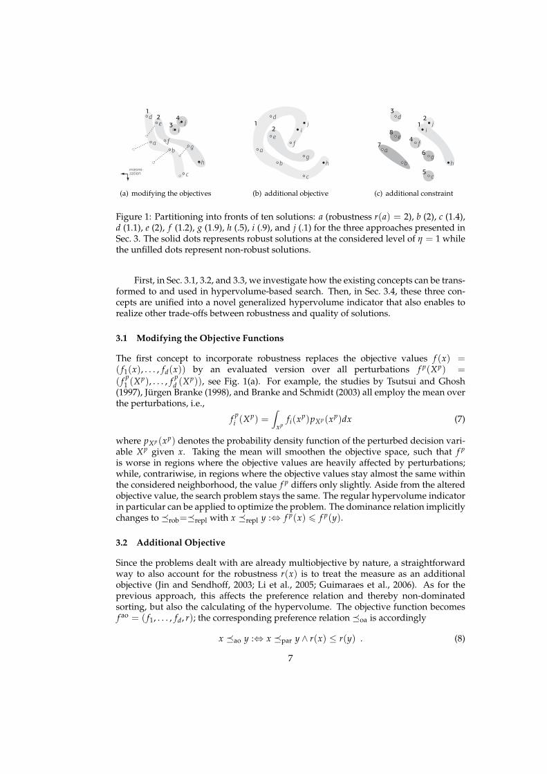
Figure 4: Partitioning into fronts of same ten solutions from Fig. 1 for the two advancedconstraint methods (a), (b), and for the generalized hypervolume indicator. The soliddots represents robust solutions at the considered level of η = 1 while the unfilled dotsrepresent non-robust solutions. For (a), solutions d, f , and c are classified robust too.

where u ∼ U(0, 1) is uniformly distributed within 0 and 1. The temperature T is expo-nentially decreased every generation, i.e., T = T0 · γg where g denotes the generationcounter, γ ∈]0, 1[ denotes the cooling rate, and T0 the initial temperature. Hence, theprobability of non robust solutions being marked robust decreases towards the end ofthe evolutionary algorithm. In the example shown in Fig. 4, the solutions d, f , and care classified as robust—although exceeding the constraint η = 1. Since these solutionsPareto-dominate all (truly) robust solutions, they are preferred over these solutions un-like in the baseline algorithm, see Sec. 3.3.

Approach 2 — Reserve Approach The second idea to overcome locally robust regionsis to divide the population into two sets: on the first one no robustness considerationsare imposed, while for the second set (referred to as the reserve) the individuals areselected according to the baseline constraint concept. This enables some individuals,namely those in the first set, to optimize their objective value efficiently. Althoughthese individuals are very likely not robust, they can improve the solutions from thesecond set in two ways: (i) a high quality solution from the first set gets robust throughmutation or crossover and thereby improves the reserve, (ii) the objective values of arobust solution are improved by crossover with an individual from the first set. How-ever, since at the end only the reserve is expected to contain individuals fulfilling theconstraint, one should choose the size of the reserve β to contain a large portion of thepopulation, and only assign few solutions to the first set where robustness does notmatter.

In detail, the reserve algorithm proceeds as follows. First, the membership of asolution to the reserve is determined; a solution x is included in the reserve, denotedby the indicator function χrsv(x), if either it is robust and there are less than β− 1 othersolutions that are also robust and dominate x; or if x is not robust but still is among theβ most robust solutions. Hence

χrsv(x) = 1 :⇔r(x) ≤ η ∧∣∣y ≼par x | y ∈ X, r(y) ≤ η

∣∣ ≤ β ∨r(x) > η ∧ |y | y ∈ X, r(y) ≤ r(x)| ≤ β

(15)

15

Given the membership to the reserve, the preference relation is:

x ≼rsv y :⇔

1 χrsv(x) = 1∧ χrsv(y) = 00 χrsv(x) = 0∧ χrsv(y) = 1x ≼par y otherwise

(16)

For the example in Fig. 4(b) let the reserve size be β = 4, leaving one additional placenot subject to robustness. Because there are fewer solutions which fulfill the robustnessconstraint than there are places in the reserve, all three robust solutions are included inthe reserve, see dashed border. In addition to them, the next most robust solution (d)is included to complete the reserve. Within the reserve, the solutions are partitionedaccording to their objective value. After having determined the reserve, all remainingsolutions are partitioned based on their objective value.

Approach 3 — Multi-Constraint Approach So far, robustness has been consideredwith respect to one robustness constraint η only. However, another scenario could in-clude the desire of the decision maker to optimize multiple robustness constraint at thesame time. This can make sense for different reasons: (i) the decision maker wants tolearn about the problem landscape, i.e., he likes to know for different degrees of robust-ness the objective values that can be achieved; (ii) the decision maker needs differentdegrees of robustness, for instance because the solution are implemented for severalapplication areas that have different robustness requirements, and (iii) premature con-vergence should be avoided.

The optimize according to multiple robustness constraints, the idea is to divide thepopulation into several groups, which are subject to a given constraint. In the follow-ing the baseline algorithm from Sec. 4.3.1 is used as a basis. The proposed concept notonly allows to optimize different degrees of robustness at the same time, but also to puta different emphasis on the individual classes by predefining the number of solutionsthat should have a certain robustness level. Specifically, let C = (η1, s1), . . . , (ηk, sl)denote a set of l constraints η1, . . . , ηl where for each constraint the user defines thenumber of individuals si ∈ N>0 that should fulfill the respective constraint ηi (ex-cluding those individuals already belonging to a more restrictive constraint). Hence,c1 + · · ·+ cl = |P|, and without loss of generality let assume η1 < η2 < · · · < ηl . Thetask of an algorithm is then to solve the following problem:

Definition 4.1 (optimal set under multiple robustness constraint). Consider C =(η1, s1), . . . , (ηk, sl), a set of l robustness constraints ηi with corresponding size si. Thena set A∗ ∈ Ψα, i.e., |A∗| ≤ α, is optimal with respect to C if it fulfills A∗ ∈ A ∈ Ψα | ∀B ∈Ψα : A 4C B where 4C is given by

A 4C B :⇔ ∀(ηi, si) ∈ C : ∀B′ ∈ Bsi ∃A′ ∈ Asi s.t. A′ 4ηi B′ (17)

where 4ηi denotes the extension of any relation proposed in Sec. 3 to sets, as stated in Eq. 9.

In order to optimize according to Def. 4.1, Algorithm 1 is proposed: beginning withthe most restrictive robustness level η1, one after another si individuals are added tothe new population. Thereby, the individual increasing the hypervolume at the currentrobustness level ηi the most is selected. If no individual increases the hypervolume, themost robust is chosen instead.

16

Algorithm 1 Classes algorithm based on the greedy hypervolume improvement prin-ciple. Beginning with the most robust class, solutions are added to the final populationP′ that increase the hypervolume at the respective level the most, given the individualsalready in P′.Require: Population P, list of constraint classes C = (η1, s1), . . . , (ηl , sl), with η1 ≤· · · ≤ ηl .

1: P′ = 2: for i = 1 to l do iterate over all classes (ηi, si) ∈ C3: for j = 1 to si do fill current class4: x′ ← arg maxx∈P\P′ Iφ(·,ηi),w

H (x ∪ P′, R)

5: if Iφ(·,ηi),wH (x′ ∪ P′, R) = Iφ(·,ηi),w

H (P′, R) then x′ has no contribution6: x′ ← arg minx∈P\P′ r(x) get the most robust instead

7: P′ ← P′ ∪ x′

8: return P′

r

a

b

c

d

d

e

(a)

r

a, 1

b, 0.9

c, 1.1

d, 0.8

d, 0.4

e, 0.5

(b)

r

a, 1

b, 0.9

c, 1.1

d, 0.8

d, 0.4

e, 0.5

(c)

Figure 5: In (a) the affected hypervolume region when removing b is shown, if robust-ness is not considered (dark gray). Adding the consideration of robustness (valuesnext to solution labels), the affected region increases (b). Foreseeing the removal of twoother solutions apart from b, other regions dominated by b might also be lost (light grayareas).

4.4 Optimizing the Generalized Hypervolume Indicator

To optimize according to the generalized hypervolume indicator, the same greedy pro-cedure as presented in Sec. 2.1 can be used. Thereby, two differences arise:

1. first off, non-dominated sorting is done according to ≼φ (Def. 3.6) and not withrespect to ≼par. In Fig. 5, for instance, the solutions d and e are in different frontsthan a for ≼par (Fig. 5(a)), but belong to the same front for ≼φ (Fig. 5(a));

2. secondly, the hypervolume loss is calculated according to the new indicator, i.e.,the loss is Iφ,w

H (A, R)− Iφ,wH (A\x, R), see gray shaded areas in Figures 5(a) and 5(b).

In this study, however, we use an advanced selection procedure introduced byHypE in Bader and Zitzler (2008, 2009). It performs regular non-dominated sorting,but uses an advanced fitness calculation scheme; rather than considering the loss whenremoving the respective solution, this scheme tries to estimates the expected loss takinginto account the removal of additional solutions, see Fig. 5(c).

17

Although the exact calculation of this fitness is possible, in this study the focusis on its approximation by Monte Carlo sampling, as also implemented in HypE. Thebasic idea is to first determine a sampling space S. From this sampling space, M sam-ples then are drawn to estimate the expected hypervolume loss. The derivation of thenecessary adjustments to consider the robustness integrating hypervolume indicatorare rather complicated and are therefore moved to the Appendix A.1. Altogether, theHypE routine to consider robustness corresponds to the regular HypE algorithm aslisted in Bader and Zitzler (2008, 2009, Algorithm 3) except for the modified fitness cal-culation. Algorithm 2 shows the new code, where only Lines 15 to 29 differ from theoriginal definition (Lines 15 to 27).

The advantage of using HypE is that the algorithms allows to also optimize manyobjective function in reasonable time. For this reason, in the experimental validationHypE will be used to optimize according to Iφ,w

H , where the desirability function φgiven in Eq. 13 is used.. The parameter θ of this function is thereby either fixed, orgeometrically decreased in each generation from 1 to θend ∈]0, 1], i.e., in generation g, θcorresponds to θg = γg with γ = gmax

√θend.

5 Experimental Validation

In the following experiments, the algorithms from Sec. 4 are compared on two test prob-lem suites and on a real world bridge truss problem presented in Appendix A.2. Thedifferent optimization goals of the approaches rule out a fair comparison as no singleperformance assessment measure can do justice to all optimization goals. Nonetheless,the approaches are compared on the optimality goal shown in Def. 3.2, which will fa-vor the constraint approach. Yet, the approach presented in Sec. 3.1 is excluded fromthe experimental comparison, since the approach is not based on a robustness measurer(x).

The following goals will be pursued by visual and quantitative comparisons:

1. the differences between the three existing approaches (see page 3) are shown;2. it is investigated, how the extended hypervolume approach performs, and how it

competes with the other approaches, in particular, the influence of the desirabilityfunction is investigated;

3. it is is examined, whether the multi-constraint approach from Sec. 4.3.2 has ad-vantages over doing independent runs or considering robustness as an additionalobjective.

5.1 Experimental Setup

The performance of the algorithms is investigated with respect to optimizing a robust-ness constraint η. The following algorithms are compared:

• as a baseline algorithm, HypE without robustness consideration, denotedHypEno. rob.;

• Algao using an additional objective;• the constraint approaches from Sec. 4.3, i.e., baseline Algcon, simulated annealing

Algsim. ann., reserve approach Algrsv, and multiple classes Algclasses;• HypE using the generalized hypervolume indicator, see Sec. 4.4.

18

Algorithm 2 Hypervolume-Based Fitness Value Estimation for Iφ,wH

Require: population P ∈ Ψ, reference set R ⊆ Z, fitness parameter k ∈ N, numberof sampling points M ∈ N. Returns an estimate of the (robustness integrating)hypervolume contributions F .

5: procedure estimateHypervolume(P, R, k, M)6: for i← 1, d do determine sampling box S7: li = mina∈P fi(a)8: ui = max(r1,...,rd)∈R ri

9: S← [l1, u1]× · · · × [ld, ud]

10: V ← ∏di=1 max0, (ui − li) volume of sampling box

11: F ← ∪a∈P(a, 0) reset fitness assignment

12: for j← 1, M do perform sampling13: choose s ∈ S uniformly at random14: if ∃r ∈ R : s ≤ r then15: p← |P| population size16: UP← ∪

a∈P, f (a)≤s f (a) solutions dominating sample s17: e← elements of UP sorted such that r(e1) ≤ · · · ≤ r(en)18: n← |UP| number of solutions dominating the sample19: for v = 0 to n− 1 do check all cutoff levels20: q← n− v− 121: α← Pv(p, q, k) probability of loss according to Eq. 2122: for f = 1 to n− v do update fitness of all contributing solutions23: if f equals n− v then least robust solution24: inc← α · (φ(r(e f ))25: else slice to less robust solution f + 126: inc← α · (φ(r(e f )− φ(r(e f+1)))

27: for j = 1 to f do update fitness28: (a, v)← (a, v) ∈ F where a ≡ e f

29: F ′ ←(F ′ \ (a, v)

)∪ (a, v + inc/ f )

30: F ← F ′31: return F

So far, the focus was on environmental selection only, i.e., the task of selecting themost promising population P′ of size α from the union of the parent and offspringpopulation. To generate the offspring population, random mating selection is used,although the principles proposed for environmental selection could also be applied tomating selection. From the mating pool SBX and Polynomial Mutation, see Deb (2001),generate new individuals.

The first test problem suite used is WFG (Huband et al., 2006), and consists of ninewell-designed test problems featuring different properties that make the problems hardto solve—like non-separability, bias, many-to-one mappings and multimodality. How-ever, these problems are not created to have specific robustness properties and the ro-bustness landscape is not known. For that reason, six novel test problems are proposedcalled BZ that have different, known robustness characteristics, see Appendix A.2.2.These novel problems allow to investigate the influence of different robustness land-scapes on the performance of the algorithms. In addition to the two test problems

19

Table 1: Parameter setting used for the experimental validation. The number of gener-ations was set to 1000 for the test problems, and to 10000 for the bridge problem.

parameter value

ηmutation 20ηcrossover 15individual mutation prob. 1individual recombination prob. 0.5variable mutation prob. 1/nvariable recombination prob. 1

continued

population size α 25number of offspring µ 25number of generations g 1000/10000perturbation δ 0.01nr. of neighboring points H 25neighborhood size δ 0.01

suites, the algorithms are compared on a real world truss building problem stated inAppendix A.2.2, where also additional results on this problem are presented. For therobustness integrating HypE, see Sec. 4.4, the variant using a fixed θ is considered (de-noted by HypEθ f ), as well as the variant with θ decreasing in each generation to θend.This latter variant is referred to as HypEθenda.

5.1.1 Experimental Settings

The parameters ηmutation and ηcrossover of the Polynomial Mutation, and SBX opera-tor respectively, as well as the corresponding mutation and crossover probabilities, arelisted in Tab. 1. Unless noted otherwise, for each test problem 100 runs of 1000 genera-tions are carried out. The population size α and offspring size µ are both set to 25. Forthe BZ robustness test problems, see Appendix A.2.2, the number of decision variablesn is set to 10, while for the WFG test problems the recommendations of the authors areused, i.e., the number of distance related parameters is set to l = 20 and the numberof position related parameters k is set to 4 in the biobjective case, and to k = 2 · (d− 1)otherwise. Except for Fig. 8, two objective are optimized.

In all experiments on the two test problem suites, the extend of the neighborhoodBδ is set to δ = 0.01. To estimate f w(x, δ), for every solution 25 samples are generatedin the neighborhood of x and f w(x, δ) is determined according to Eq. 6. After eachgeneration, all solutions are resampled, even those that did not undergo mutation. Thisprevents that a solution which, only by chance, reaches a good robustness estimate,persists in the population. For the real world bridge problem, on the other hand, aproblem specific type of noise is used that allows to analytically determine the worstcase, see Appendix A.2.1.

For the Algsim. ann. approach the cooling rate γ is set to 0.99. The reference set of thehypervolume indicator is set to R = r with r = (3, 5) on WFG, with r = (6, 6) onWFG, and with r = (0, 2000) on the bridge problem5. The Algclasses-approach proposedin Sec. 4.3.2 uses the following constraints: for BZ (η1, . . . , η5) = (.01, .03, .1, .3, ∞).For WFG, due to generally higher robustness levels on these test problems, the classeswere set to (η1, . . . , η5) = (.001, .003, .01, .03, ∞). In both cases, the class sizes were(s1, . . . , s5) = (4, 4, 6, 4, 6) which gives a populations size of 24. For the bridge problem,the classes are set to (.001, .01, .02, 0.1, ∞) with 6 individuals in each class. The size of

5For this problem, the first objective is to be maximized.

20

the bridge is set to 8 decks, i.e., spanning a width of 40 m. For comparison with a singleconstraint it is set to η = 0.02. For each comparison, 100 runs of 10000 generations havebeen performed.

In this paper, two types of uncertainty are used. Firstly, for the test problems,where x ∈ Rn holds, Xp is assumed to be uniformly distributed within Bδ(x) accordingto Eq. 4. Random samples are generated within Bδ(x), and evaluated to obtain anestimate of the robustness measure r(x). Secondly, for the real world application, aproblem specific type of noise is considered as outlined in Appendix A.2.1. For thissecond type of noise, along with the structure of the problem, the worst case can bedetermined analytically.

5.1.2 Performance Assessment

For all comparisons, the robustness of a solutions has to be assessed. To this end, 10000samples are generated within Bδ. For each objective separately, the 5% largest valuesare then selected. By these 500 values, the tail of a Generalized Pareto Distribution isfitted, see S. Kotz and S. Nadarajah (2001). The method of moments is thereby used toobtain a first guess, which is then optimized maximizing the log-likelihood with respectto the shape parameter k and the logarithm of the scale parameter, log(σ)6. Given anestimate for the parameters k and σ of the Generalized Pareto Distribution, the worstcase estimate f w

i (x) is then given by

f wi (x) =

θ − σ/k k < 0∞ otherwise

(18)

where θ denotes the estimate of the location of the distribution given by the smallestvalue of the 5% percentile.

The performance of algorithms is assessed in the following manner: at first, a vi-sual comparison takes place by plotting the objective values and robustness on thetruss bridge problem Appendix A.2.1. The influence of θ of the robustness integratingHypE is then further investigated on BZ1. Secondly, all algorithms are compared withrespect to the hypervolume indicator at the optimized robustness level η. To this end,the hypervolume of all robust solutions is calculated for each run. Next, the hypervol-ume values of the different algorithms are compared using the Kruskal-Wallis test andpost hoc applying the Conover-Inman procedure to detect the pairs of algorithms be-ing significantly different. The performance P(Ai) of an algorithm i then correspondsto the number of other algorithms, that are significantly better. See Bader and Zitzler(2008, 2009) for a detailed description of the significance ranking. The performance Pis calculated for all algorithms, on all test problems of a given suite.

In addition to the significance rank at the respective level η, the mean rank of analgorithm when ranking all algorithms together is reported as well. The reason forplotting the mean rank instead of the significance is to also get an idea of the effect sizeof the differences—due to the large number of runs (100), differences might show upas significant although the difference is only marginal. The mean rank is reported not

6Note that the maximum likelihood approximation is only efficient for k ≥ −1/2 (S. Kotz and S. Nadara-jah, 2001). Preliminary studies, however, not only showed k ≥ −1/2 for all test problems considered, butalso revealed that k is the same for all solutions of a given test problem.

21

0

10

20

0100200300

(a) no robustness

0

10

20

0100200300

(b) additional objective

0

10

20

0100200300

(c) classes

0

10

20

0100200300

(d) reserve

0

10

20

0100200300

(e) constraint

0

10

20

0100200300

(f) HypE.001a

Figure 6: Pareto front approximations on the bridge problem for different algorithms.Since the first objective of the bridge problem, the structural efficiency, has to be maxi-mized, the x-axis is reversed such that the figure agrees with the minimization problem.The robustness of a solution is color coded, lighter shades of gray stand for more ro-bust solution. The dotted line represents the Pareto front of robust solutions (for (a), norobust solutions exists).

00

1 1.6 2

1

1.6

2

(a) HypE with fixed θ = 0.8

00

1 1.6 2

1

1.6

2

(b) HypE with fixed θ = 0.1

00

1 1.6 2

1

1.6

2

(c) HypE with fixed θ = 0.001

Figure 7: Solutions of 100 runs each on BZ1. The dotted line indicates the Pareto front,the dashed line the best robust front.

only for the optimized level η, but a continuous range of other robustness levels as wellto get an idea of the robustness distribution of the different algorithms.

22

Table 2: Comparison of HypE.001a and HypE.1f to different other algorithms for the hy-pervolume indicator. The number represent the performance score P(Ai), which standsfor the number of contenders significantly dominating the corresponding algorithm Ai,i.e., smaller values correspond to better algorithms. Zeros have been replaced by “·”.

Alg

ao

Alg

con

Alg

clas

ses

Hyp

E .00

1a

Hyp

E .1f

Hyp

E no.

rob.

Alg

rsv

Alg

sim

.ann

.

BZ1 6 · 5 · · 7 3 4BZ2 4 7 2 2 4 · · 5BZ3 · 1 1 2 2 7 3 1BZ4 2 5 1 3 4 7 · 6BZ5 4 · 4 · · 7 1 6BZ6 · 4 2 4 4 5 1 2

WFG1 4 1 · 1 4 7 1 4WFG2 5 7 · 1 1 4 1 1WFG3 1 2 · 2 3 3 2 2WFG4 6 3 · 1 3 6 2 2WFG5 6 1 · 1 1 7 2 3WFG6 6 1 3 · · · · ·WFG7 7 · 5 · · 4 3 ·WFG8 6 3 6 · · 1 · 2WFG9 6 1 · 1 1 6 4 5

Bridge 4 1 4 1 · 3 7 4 6Bridge 6 3 4 2 · · 7 4 6Bridge 8 3 5 2 1 · 7 4 5Bridge 10 3 4 2 · · 7 3 5Bridge 12 4 4 2 1 · 7 2 4

Total 77 57 38 20 30 106 40 69

5.2 Results

5.2.1 Visual Comparison of Pareto fronts

First, the algorithms are compared visually on the bridge problem (see Appendix A.2.1with 8 decks. Fig. 6 shows the undominated solutions—according to relation x ≼ao yin Eq. 8 on page 7—of 100 runs for algorithms presented in Sec. 4.

As the Pareto-set approximations in Fig. 6 show, a comparison of the different ap-proaches is difficult: depending on how robustness is considered, the solutions exhibitdifferent qualities in terms of objective values and robustness. It is up to decision makerto chose the appropriate method for the desired degree of robustness. The existing threeapproaches thereby constitute rather extreme characteristics. As the name implies, theHypEno. rob. approach only finds non-robust solutions, but in exchange converges fur-ther to the Pareto optimal front. However, the approaches Algao, Algclasses, and Algrsvconsidering robustness (at least for some solutions), outperform HypEno. rob. in some

23

regions even with respect to non-robust solutions: the Algrsv finds better solutions forlow values of f2, while the other two approaches outperform the HypEno. rob. algorithmon bridges around f2 = 10 m. Considering robustness as an additional objective leadsto a large diversity of robustness degrees, however, misses solutions with small valuesof f2. This might be due to the choice of the reference point of the hypervolume indi-cator, and the fact that only 25 solutions are used. The Algclasses algorithms optimizesfive robustness degrees, two of which are classified as non-robust—these two are lyingclose together because the robustness level of the second last class with η4 = 0.1 doesbarely restrict the objective values. Despite—or perhaps because of—the Algrsv algo-rithm also keeping non-robust solutions, the robust front is superior to the one of theAlgcon algorithm. The HypE approach with θ decreasing to .001 advances even further.The result of the Algsim. ann. algorithm does not differ much from the Algcon approachand is therefore not shown.

5.2.2 Influence of the Desirability Function φ

As the previous section showed, the robustness integrating HypE seems to, at least forsmall θ, have advantages over the Algcon. Another advantage is its ability to adjust thetrade-off between robustness and objective value quality. Fig. 7 shows the influence ofdifferent θ on the robustness and quality of the found solutions on BZ1. For this testproblem, the robustness of solutions increases with distance to the (linear) Pareto front,see Appendix A.2.2. The new indicator allows to realize arbitrary trade-offs betweenrobustness and objective values, ranging from solutions with good objective value tovery robust solutions. In the present example, only when choosing θ < 0.1, solutionsrobust at the constraint level are obtained. In the following a version with θ fixed to 0.1is used (referred to as HypE.1f), and a version with θ decreasing to 0.001 (referred to asHypE.001a).

5.2.3 Performance Score over all Test Problems

To obtain a more reliable view of the potential of the different algorithms, the compar-ison is extended to all test problems. To this end, the performance score P(Ai) of analgorithm i is calculated as outline in Sec. 5.1.2. Tab. 2 shows the performance on the sixBZ, the nine WFG, and five instances of the bridge problem. Overall, HypE.001a reachesthe best performance, followed by HypE.1f, Algclasses, and Algrsv. four algorithms showa better performance than Algcon.

Hence, not only are two modifications of the constraint approach (Algclasses, Algrsv)able to outperform the existing constraint approach, but the robustness integrating hy-pervolume indicator as well is overall significantly better than Algcon.

On the bridge problem, HypE.001a performs best and is significantly better thanthe other three algorithms. In case of Algrsv, and Algcon, it is better in nearly 100% ofall runs. On WFG, Algclasses overall performs best. An exception is WFG6-8, where theother three algorithms are all better. On BZ1, 3 and 5, HypE.001a and Algcon performbest, on the remaing BZ problems Algrsv works best.

5.2.4 Application to Higher Dimensions

All algorithms proposed are not restricted to biobjective problems, but can also be usedon problems involving more objectives. Since the runtime increases exponentially with

24

.3

.4

.5

.6

2 3 4 5 7 10 15 30 5020

constraint HypE.1f

additionalobjective

no robustness

reserve

HypE.001a

mea

n ra

nk (b

ette

r→)

nr. of objectives

.2

Figure 8: Average Kruskal-Wallis ranks over all WFG test problems at the robustnesslevel η = 0.01 for different number of objectives.

0

.25

.5

.75

¼ ½ 0.9 1 1.1 2 4 ∞

classes

classes

constraint

simulatedannealing

no robustness

HypE.1f

HypE.1f

HypE.001aadd. objective

add. obj.add. obj. HypE.001a no rob.

robustness level (normalized to η)

mea

n ra

nk (b

ette

r→)

Figure 9: Average Kruskal-Wallis ranks over all BZ, WFG, and bridge test problemscombined for different degrees of robustness. The best algorithm for a particular ro-bustness level are indicated on top.

25

the number of objectives, HypE is applied to optimize the hypervolume when facingmore than three objectives. Fig. 8 shows the mean Kruskal-Wallis rank for a selectedsubset of algorithms at different number of objectives. The algorithm HypE.001a showsthe best performance except for 10 objectives, where the mean rank of the Algrsv ap-proach is larger (although not significantly). Except for 7 and 20 objectives, HypE.001ais significantly better than Algcon. On the other hand, HypE.1f performs worse thanthe constraint approach for all considered number of objectives except the biobjectivecase. This might indicate, that the parameter θ in Eq. 3 needs to be decreased withthe number of objectives, because the trade-off between objective value and robustnessis shifted towards objective value for larger number of objectives. However, furtherinvestigations need to be carried out to show the influence of θ when increasing thenumber of objectives.

5.2.5 Performance over Different Robustness Levels

In the previous comparisons, solutions robust at the predefined level have been con-sidered. What happens if loosening or tightening up this constraint? Fig. 9 illustratesthe mean hypervolume rank, normalized such that 0 corresponds to the worst, and 1 tothe best quality. The mean ranks are shown for different levels of robustness ρ, normal-ized such that the center corresponds to the level optimized. For levels of robustnessstricter than η, the Algclasses approach reaches the best hypervolume values. Around η,HypE.001a performs best and further decreasing the robustness level, HypE.1f overtakes.Further decreasing the robustness, Algao, and finally HypEno. rob. are the best choices.

5.2.6 Optimizing Multiple Robustness Classes

Although the Algclasses approach proved useful even when only one of its optimizedclasses are considered afterwards, the main strength of this approach shows when ac-tually rating the hypervolume of the different classes optimized. Tab. 3 list the signif-icance rankings for the different classes averaged over all test problems of BZ, WFG,and truss bridge. Doing Algind. runs is significantly worse than the remaining approachesconsidered. This indicates, that optimizing multiple robustness levels concurrently isbeneficial regardless of the robustness integration method used. Overall, the Algclassesapproach reaches the best total significance score (69), the algorithms scores best on allclasses except the one without robustness (η = ∞), where the HypEno. rob. outperformsthe other algorithms.

6 Conclusions

This study has shown different ways of translating existing robustness concepts tohypervolume-based search, including (i) the modification of objective values, (ii) theintegration of robustness as an additional objective, and (iii) the incorporation of ro-bustness as an additional constraint. For the latter, three algorithmic modifications aresuggested to overcome premature convergence. Secondly, an extended definition of thehypervolume indicator has been proposed that allows to realize the three approaches,but can also be applied to more general cases, thereby flexibly adjusting the trade-offbetween robustness and objective values while still being able to focus on a particularrobustness level. To make this new indicator applicable to problems involving a largenumber of objectives, an extension of HypE (Hypervolume Estimation Algorithm for

26

Table 3: Comparison of the algorithms: Algind. runs, Algao, HypEno. rob., and Algclasses. Foreach optimized class the sum of the performance score is reported for each of the threeconsidered problem suites BZ, WFG, and the bridge problem.

Algind. runs Algao HypEno. rob. Algclasses

.01 BZ 0 3 3 3Bridge 8 10 3 3

.001 WFG 3 5 8 2

.03 BZ 10 4 17 2Bridge 8 10 1 4

.003 WFG 8 11 13 6

.1 BZ 13 4 17 1Bridge 8 10 1 4

.01 WFG 13 15 12 5

.3 BZ 10 4 17 2Bridge 10 8 0 5

.03 WFG 18 12 12 6

∞BZ 17 9 3 5Bridge 12 6 1 5WFG 27 11 1 14

Total 177 135 112 69

Multiobjective Search) (Bader and Zitzler, 2008, 2009) has been presented.

The main results of this study can be summarized as follows:

• The three above mentioned approaches each have their advantages: modifyingthe objective values allows to use existing approaches without increasing the com-plexity of the problem; using an additional objective yields to a large diversityof different degrees of robustness, while using an additional constraint allows tofocus on one desired robustness level.

• The existing constraint approach can be improved by the proposed algorithmicmodifications, in particular by the reserve approach and by optimizing multipleclasses; the latter furthermore illustrates that if all desired classes of robustnessare known, it is better to optimize those concurrently instead of doing multipleindependent runs or to generally consider robustness as an additional objective.

• The novel robustness integrating hypervolume indicator seems to offers many ad-vantages: first, the concept allows to realize not only the three existing approaches,but also other arbitrary trade-offs the decision maker expresses. Second, this newapproach—if concentrating on a single robustness constraint—is able to producebetter solutions than the baseline constraint approach.

The investigations presented in this paper are not only valuable in the robustnesscontext; in fact, they represent general ways to incorporate additional criteria and con-straints in hypervolume-based search. A promising direction for future research is inparticular how multiple (and not only a single) constraints can be integrated in a gen-eral manner.

27

A Appendix

A.1 HypE for the Generalized Hypervolume Indicator

The complexity of calculating the regular hypervolume is ♯P complete as proven byBringmann and Friedrich (2008). The complexity for the generalized hypervolume in-dicator, see Eq. 12, is even increased.

For this reason, an approximation scheme has to be used to exploit the potentialof the robustness integrating hypervolume indicator for larger number of objectives.To this end, in the following section HypE, introduced in Bader and Zitzler (2009), isextended.

Introducing Robustness to HypE HypE needs to be modified in order to be applica-ble to the robustness integrating hypervolume indicator (Def. 3.5) due to the followingobservations. In case of the regular hypervolume indicator, a dominated region is ac-counted 100% as long as at least one point dominates it. So the only case HypE has toconsider is removing all points dominating the portion altogether. For different pointshaving different degrees of robustness, the situation changes: even though a partitiondominated by multiple points would stay dominated if one removes not all dominatingpoints, the robustness integrating hypervolume might nevertheless decrease due to thenon bivariate attainment function. For example, if the most desirable point in terms ofrobustness is removed, then the attainment function is decreased and thereby also thehypervolume indicator value, see Theorem 3.7.

The second difference to the original HypE algorithm concerns the way the contri-bution is shared among the dominating point. For the regular hypervolume indicator,all solutions dominating the considered region are equally valuable since they entailthe attainment function being 1. Consequently, the region is split equally among all so-lutions. For example, if four solutions dominate a region, the fitness of each is increasedby 1/4 of the volume of the region, see Fig. 10(a). For the robustness integrating hy-pervolume indicator, one has to distinguish different layers of robustness, which areachieved by subsets of all individuals dominating the region. Consequently, the hy-pervolume of these layers should only be split among those solutions actually reachingthat robustness level, see Fig. 10(b). In the following, first the question is tackled of howto distribute the layers of robustness of a dominated portion among solutions. Then theprobability is derived, that each one of these layers is lost.

Distributing Hypervolume among Solutions Let A denote the set of points andUP ⊆ A those solutions, that dominate the region U under consideration. To illus-trate the extended calculation of the robustness integrating HypE, consider ten pointsA = x1, . . . , x10. The first four points UP = x1, . . . , x4 dominate the regionU = H(x1, . . . , x4, x1, . . . , x10, R). Additionally, let r(x1) ≤ r(x2) ≤ r(x3) ≤ r(x4).First, a few simple cases are considered before presenting the final, and rather intrigu-ing, formula to calculate the fitness of a point. First of all, it is investigated how muchthe robustness integrating hypervolume Iφ

A decreases when removing points from theset UP and how to attribute this loss to individuals. Assume x2 or any other pointwhich is less robust than x1 is removed. In this case, the robustness integrating hy-pervolume does not decrease at all, since the attainment function depends only on themost robust point dominating the partition, in our case on x1. Hence, a removal only

28

¼

0

1

φ

dominated area

(a) regular HypE

½

1

¼four

three

two

onenone

number of pointsreaching the robustness:

⅓

(b) robustness integrating HypE

Figure 10: Illustrates how a portion of the objective space U is attributed to the most ro-bust among four points dominating the region. In case of no robustness considerations,the solutions all get 1/4 of λ(U) as every other solution, see (a). When considering ro-bustness, different layers of robustness have to be distinguished, see (b): the first, andmost robust, layer is dominated by no point, and is therefore disregarded. Only themost robust solution dominates the second layer, hence gets the whole slice. The thirdlayer is dominated by an additional point, and both solutions get half of the share. Theprocedure continues up to the layer where every point reaches the necessary robust-ness, this layer is distributed evenly among all points.

affects the hypervolume, if no other point dominating the partition U at least as robustas the removed point remains in the population.

On the other hand, lets assume only the most robust solution x1 is removed. Bydoing this, the hypervolume decreases by λ(U) · (φ(r(x1)) − φ(r(x2))), which is nonzero if the robustness of x1 is more desirable than the one of x2. Clearly, this loss hasto be fully attributed to point x1, as no other point is removed. Now lets extend thisto more than one point being removed. Assume points x1, x2, and x4 are removed.As seen before, the loss of x4 does not affect the hypervolume since x3 (which is morerobust) stays in the set. So in a set of points remaining in the population, the mostrobust individual sets a cutoff. For all individuals above this cutoff, i.e., for all indi-viduals being less robust, the hypervolume does not decrease if these individuals areremoved. The total loss of Iφ,w

H is λ(U) · (φ(r(x1)) − φ(r(x3))). The question now is,how to distribute the loss among solutions. The share λ(U) · (φ(r(x1))− φ(r(x2))) isonly due to x1, hence it is fully attributed to x1. The share between φ(x2) and φ(x3) isdominated by both x1 and x2, so the portion is evenly split. This procedure continuesfor all robustness levels below the cutoff, see Fig. 10(b).

Probability of Loosing Hypervolume Now that it is known how to distribute thepartition U among points for a particular selection of points, one has to consider allpossible subsets of UP, i.e., subsets of points dominating U, and calculate the prob-ability that the subset is lost. Let p denote the total number of points, let n := |UP|denote the number of points dominating U, and let k denote the number of points tobe removed, i.e., k = p− α. Not all (n

k) subsets have to be considered separately, butthey can be summarized into classes ci with 0 ≤ i ≤ n − 1, where i denotes the po-sition of the cutoff level, see Fig. 11. More specifically, cv contains all subsets where

29

p points in total

n solutions in set UP

vq

- - - -+ + + +

k poinst removed (-)

cutoff point

consideredloss

sorted according torobustness

most robust of UP

least robust of UP

Figure 11: Illustration of class cm: from p points, n dominate the region under consid-eration. The cutoff point is denoted as v. Besides the considered solution, q points needto be removed below the cutoff. In total k points are removed. In the example, p = 9,v = 2, q = 2, n = 5, and k = 5.

the most robust solution from UP not being removed is the vth least robust solutionamong all solutions in UP. For v = 0, all solutions dominating U are removed. Forexample, let (χ1, . . . , χp) represent different subsets of A, where χi ∈ 0, 1 denotes theabsence or presence respectively of solution xi, and χi = × denotes both cases (don’tcare). In the considered example, c0 = (0, 0, 0, 0,×, . . . ,×), c1 = (0, 0, 0, 1,×, . . . ,×),c2 = (0, 0, 1,×,×, . . . ,×), and c3 = (0, 1,×,×,×, . . . ,×). Note that as for the regularHypE calculation, the fitness of a solution is determined under the assumption thatthis solution is removed, therefore, the subset c4 (no solution removed from UP) is notpossible.

To derive the probability that a subset being removed belongs to the class cm, con-sider one particular way this can happen: the first q individuals are removed frombelow the cutoff, i.e., are more robust. The remaining k − q points are then removedfrom above the cutoff or from the set A\UP. This is one of (k−1

q ) equally probable com-binations to obtain a cutoff level v, so that the obtained probability has to be multipliedby (k−1

q )7 in the end.

A cutoff of v means, besides the considered point q = n− v− 1 points are removedfrom below the cutoff level. The probability that these q individuals are removed in thefirst q removal steps is:

P1 =q

p− 1· q− 1

p− 1· · · 1

p− q=

q! · (p− 1− q)!(p− 1)!

. (19)

For the remaining k − 1 − q points, any of the p − n individuals not dominating thepartition may be selected, as well as any of the v− 1 individuals above the cutoff, i.e.,solutions less robust than the cutoff. The cutoff itself may not be removed as this wouldchange the level v. So the probability for the second portion of points to be pickedaccordingly is:

P2 =p− n + v− 1

p− q− 1· p− n + v− 2

p− q− 2· · · p− k

p− k + 1=

(p− n + v− 1)!(p− k)!(p− k− 1)!(p− q− 1)!

(20)

7Again, note that the solutions whose fitness needs to be determined, is assumed to be removed andbelongs to the first q individuals, otherwise it would induce no loss in hypervolume. That is why the binomialcoefficient considers the k-1 set instead of k.

30

Multiplying P1 (Eq. 19), P2 (Eq. 20) and the number of combinations (k−1q ) gives the

final probability

Pv(p, q, k) = P1 · P2 ·(

k− 1q

)=

(p− k)!(p− 1)!

· q! · (p− q− 2)!(p− k− 1)!

· (k− 1)!q!(k− 1− q)!

= (p− 1)(p− q− 2)!(p− 1)!

(k− 1)!(k− 1− q)!

= (p− 1)p−1

∏i=p−q−1

1i

k−1

∏i=k−q

i . (21)

For v = 0 and p = n the last line is undefined, in this case, P0(n, q, k) = 1 holds.

Example A.1. Consider four solutions a, b, c and d with robustness r(a) = 0.8, r(b) = 0.9,r(c) = 1.05 and r(d) = 1.2. Let the robustness constraint be η = 1, and let the desirabilityφ be defined according to Eq. 13 with θ = 0.1 and assume two solutions need to be removed.Now consider a sample dominated by a, c and d. This gives p = 4, n = 3 and k = 2.Since only two individuals are to be removed, the probability for having v = 0, i.e, all threeindividuals dominating the sample are removed, is 0. The probability for v = 1, i.e., anothersolution dominating the sample is removed besides the considered individual, is 1/3. In thiscase, the first robustness layer extends from r(a) = .8 to r(c) = 1.05. This gives a value of13(

φ0.1(.8)− φ0.1(1.05))= 0.253 which is completely attributed to a since only this solution

reaches the degree of robustness. The second layer extends from r(c) = 1.05 to r(d) = 1.2and half of the value 1

3(

φ0.1(1.05) − φ0.1(1.2))= 0.079 is added to the fitness of a and c

respectively. The probability for v = 2 is 2/3 (either b or d can be removed, but not c). Thecontribution 2

3(

φ0.1(.8)− φ0.1(1.05))= 0.506 is completely added to the fitness of a.

A.2 Test Problems

In this appendix two new classes of problems for robustness investigations are pre-sented: first, in Sec. A.2.1 a real world mechanical problem is stated. Secondly, inSec. A.2.2 a novel test problem suite is presented to test the performance of algorithmswith respect to different robustness landscapes.

A.2.1 Truss Bridge Problem

First, the truss bridge problem is stated. Then, a problem-specific evolutionary algo-rithm is presented.

Problem Statement The task is to build a bridge over a river. Between two banks, nequally long decks have to be supported by a steel truss8. A uniform load is assumedover the decks that lead to n− 1 equal force vectors, see Fig. 12. The first objective of thetruss problem is to maximize the structural efficiency—the ratio of load carried by thebridge without elastic failure to the total bridge mass, i.e., costs. The river is consideredenvironmentally sensitive and therefore no supporting structures are allowed belowthe water level. Furthermore, to limit the intervention in the natural scenery, the secondobjective is to minimize the rise of the bridge, measured from the decks at the center ofthe bridge9.

8The decks are of 5 meters long.9The height is arbitrarily defined at the middle of the bridge and not over the entire span width, to pro-

mote bridges very different to those optimizing the structural efficiency, and which tend to have the largestheight at the center of the bridge.

31

right side mirrored

water level

fixed nodes

n decks load L

intial bridge: warren truss

Figure 12: Illustration of the truss bridge problem. Between the two banks with pre-defined abutments, n decks with equal load have to be supported by a steel truss. Asstarting point, the individuals of the evolutionary algorithm are initialized to the shownWarren truss without verticals. At each bank, two supplementary fixed nodes are avail-able to support the bridge additionally.

The bridge is considered two dimensional, i.e., all nodes and bar lie within a twodimensional plane. The slender members (referred to as bars) are connected at revolutejoints (referred to as nodes). Half of the external load on the decks is applied to each ofthe two end joints and the weight of the members is considered insignificant comparedto the loads and is therefore omitted. Hence, no torsional forces are active and all forceson members are tensile or compressive. For detailed information on truss bridges seeW.F. Chen and L. Duan (1999).

In contrast to other well known truss problems, like for instance the ten bar trussproblem (Deb, 2001), the nodes or bars are not specified in advanced, neither are theyrestricted to discrete positions like as in Ben-Tal and Nemirovski (2003). In fact, allkinds of geometries are possible which renders the problem much harder than theabove mentioned ten bar truss problem. The only restriction is, that the predefineddecks can not be changed in any way. In addition to the two endpoints, two additionalfixed nodes at each bank can, but do not need to be, added to the truss10.

The truss is made only from steel with yield strength 690 MPa and density7800 kg/m3. The maximum area of the members is 0.04 m2 (radius 0.2 m), and the mini-mum area is set to 2.5·10−5 m2, (radius of 5 mm). The decks have a fixed cross-sectionalarea of 0.02 m2.

Evolutionary Algorithm In the following an evolutionary algorithm is presented tai-lored to the steel truss bridge problem stated above. The algorithm consists of (i) ageneral representation which can model all possible bridges, (ii) an initialization of so-lutions, (iii) the calculation of the objective values, and (iv) different mutation operatorsto generate new solutions.

Representation The representation consists of variable length lists. The first list con-tains all nodes. A node is thereby determined by its position (x, y), the degrees offreedom of the node (i.e., whether the node is fixed or not), and the load attached tothis node—the latter is non-zero only for the n− 1 predefined joints between the decks.The second list contains the members that consist of references to the two endpoints,and the cross-sectional area of the bar. Since the problem is mirror-symmetrical, only

10The additional fixed nodes are located 2.5 m below the edge of the abutment and 7.5 m to the left andright of the edge respectively.

32

moving member

changing barthickness

removing node adding member adding fixed node

removing member moving node breaking triangle &moving the node

Figure 13: Illustrates the eight mutation operators used to optimize the bridge problem.

the left half of the bridge is represented and solved, see below.

Initialization As a starting point, all solutions are set to a Warren truss without ver-ticals, and with equilateral triangles. This ensures that the initial bridges are staticallydeterminate and stable. Of course, the risk increases that the diversity of solutions islimited unnecessarily. As the results in Sec. 5.2 on page 23 show this is not the casethough—the solutions found vary a lot from the initial Warren truss.

Calculating the Objective Function To determine the first objective function, thestructural efficiency, matrix analysis of the truss is performed; more specifically, thematrix force method is used to determine the internal forces of all members. Giventheir area, the weakest link can then be identified which defines the maximum load ofthe bridge. If the bridge is statistically undetermined, i.e., the matrix becomes singular,the bridge is classified infeasible. No repairing mechanism is used in this case. Theweight of the bridge, on the other hand, is determined by summing up the product oflength, area, and density of all bars. For the weight, the members constituting the deckof the bridge are also included. Finally, dividing the maximum load by the densitygives the first objective, i.e., the structural efficiency.

The maximum vertical distance of a member or node above the deck level, mea-sured at the center of the bridge, gives the second objective. The rise of the bridge is tobe minimized.

Because of the symmetry of the problem, only the left half of the bridge is repre-sented and solved. To this end, all nodes lying on the mirror axis, the center of thebridge, are fixed in the horizontal dimension. This models the fact, that due to symme-try, the horizontal component of the force vectors at these nodes is zero. All membersexcept those on the mirror axis are considered twice in terms of cost, since they have asymmetric counterpart. On the other hand, the internal load of members on the sym-metry axis is doubled after matrix analysis, since the right, not considered, half of thebridge will contribute the same load as the left half.

Mutation Operators Due to the complex representation of the bridges no crossoverbut only mutation operators are applied to generate new bridges. In each generation,one of the following eight mutation functions is used, where the probability of an op-erator is evolved by self-adaptation (Deb, 2001):

33

moving member A member is randomly picked and its endpoints are changed, suchthat the member ends up at a different place.

removing member A randomly chosen member is removed. Nodes that are no longerconnected are removed too.

adding member Two nodes are picked randomly and a member is added betweenthem.

moving nodes The location of a node is moved uniformly within the interval [-1 m,1 m]×[-1 m,1 m].

removing node A randomly chosen node is removed; all members connected to thatnode are removed as well.

adding fixed node A node from the set of fixed nodes is picked, and connected to arandomly chosen (non-fixed) node.

breaking triangle and moving node This mutation operator should help the forma-tion of repeated triangular patterns, which are known to be beneficial because tri-angles can not be distorted by stress. An existing triangle is chosen, then one ofits three sides is divided in the middle by adding a new node. This node is thenconnected by the corresponding median of the triangle. Since this new memberwould get zero force, the new node is moved additionally by the operator movingnode.

changing member area This mutation operator randomly picks a member andchanges its area by factor ρ, where ρ ∼ U(0.5, 1.5) is randomly distributed be-tween 0.5 and 1.5.

Fig. 13 illustrates the eight mutation operators. In addition to these operators, with aprobability of 50% the cross-sectional areas of the bridge are optimized according tomatrix analysis, i.e., each cross-sectional area is decreased as far as the maximum loadcarried does not decrease.

Noise Many different sources of uncertainty are conceivable for the truss problem,e.g., differing location of the nodes due to imprecise construction, varying memberarea because of manufacturing imperfection or changing external load distributions.The present thesis considers random perturbations of the yield strength of members.The thicker a bar thereby is, the larger the variance of the noise. The reasoning behindthis assumption is that material properties are harder to control the larger a structureis. The model σUTS ∼ σUTS · U(1− (r2)δ, 1 + (r2)δ) is used, where r is the radius ofthe bar and σUTS denotes the yield strength of a member. As robustness measure, themaximum deviation according to Eq. 5 is used. However, in contrast to Sec. 5 wherea sampling procedure is used to estimate the worst case, the worst case is determinedanalytically: for each member, the yield strength is set to the minimum value accordingto the noise model, i.e., σw

UTS = σUTS · (1− (r2))δ. In all experimental comparisons, δwas set to 100.

A.2.2 BZ Robustness Test Problem Suite

Existing test problem suites like WFG (Huband et al., 2006) or DTLZ (Deb et al., 2002b)feature different properties—like non-separability, bias, many-to-one mappings andmultimodality. However, these problems have no specific robustness properties, andthe robustness landscape is not known. For that reason, six novel test problems areproposed denoted as Bader-Zitzler (BZ) that have different, known robustness charac-teristics. These problems, BZ1 to BZ6, allow to investigate the influence of different

34

robustness landscapes on the performance of the algorithms. All, except for BZ5, sharethe following simple structure:

Minimize fi(x) =xi

∥∑ki=1 xi∥β

·(1 + S(g(x))

)1 ≤ i ≤ d

with g(x) =1

n− k

n

∑i=k+1

xi

subject to 0 ≤ xi ≤ 1 for i = 1, 2, . . . , n

(22)

The first k decision variables are position related, the last n− k decision variables deter-mine the distance to the Pareto front. The Pareto front is reached for xi = 0, k + 1 ≤ i ≤n, which leads to S(g(x)) = 0. The front has has the form

(f1(x)β + . . . + fd(x)β

)1/β=

1. The parameter β thereby specifies the shape of the Pareto front: for β > 1 the shapeis convex, for β = 1 it is linear and for 0 < β < 1 the shape is concave. The distanceto the Pareto front is given by S(g(x)), where g(x) is the mean of the distance relateddecision variables xk+1, . . . , xn (an exception is BZ5, where S is a function of g(x) andthe variance σ2 = Var(x1, . . . , xk)).

The distance to the front, i.e., S(g(x)), depends on a fast oscillating cosine functionthat causes the perturbations of the objective values and where its amplitude deter-mines the robustness of a solution. In the following, realization of S are listed, andchoice of parameter β for the six test problems BZ1 to BZ6 and discuss their robustnesslandscape.

In the following, let h := g(x)

BZ1 For the first test problem, the distance to the front subject to h := g(x) is

S(h) = h +((1− h) · cos(1000h)

)2 (23)

Fig. 14(a) shows the function S as a function of h, as well as the maximum and mini-mum within a neighborhood of Bδ (see Sec. 2.2). As for all BZ test problems, the (bestcase) distance to the front linearly decreases with decreasing d. The difference to theworst case, on the other hand, goes in the opposite direction and increases. This givesa continuous trade-off between the objective values f (x) (better for smaller values of h)and the robustness r(x) (better the larger h). The parameter β is set to 1 which gives alinear front shape.

BZ2 For the second test problem, β = 2 describing a sphere-shaped Pareto front, thedistance to which is given by:

S(h) = 3h +1

1 + exp(−200(h− 0.1))·((1− h) · cos(1000h)

)2 (24)

Fig. 14(b) shows the distance as a function of h. As in BZ1, the robustness first decreaseswith decreasing h. However, around h = 0.1 the exponential distribution kicks in, andthe amplitude of the cosine function becomes very small such that the Pareto front andits adjacencies are robust. BZ2 tests, whether an algorithm is able to overcome thedecreasing robustness as approaching the Pareto front, or if the solutions are drivenaway from the Pareto front to increase their robustness.

35

0 10

2

worst case within δ=0.01

best case within δ=0.01

f(x)

dist

ance

g(x)

(a) BZ1

0 10

1

2

3

(b) BZ2

0 10

1

2

(c) BZ3

0 10

1

2

(d) BZ4

0 10

1

2Part 1

Part 2

(e) BZ5

0 10

1

2

(f) BZ6

Figure 14: Distance to the front (gray line) as a function of g(x) (abscissa), see Eq. 22.The solid and dashed line represent the minimal and maximal distance respectivelywithin the interval [g(x− δ), g(x + δ)] with δ = 0.01.

BZ3 For the third instance of BZ the distance to the front is a product of two cosineterms:

S(h) = h +(

cos(50h) cos(1000h))4 . (25)

The concave Pareto front (β = 0.5) is non robust. However, by increasing the distanceto the front the term cos(50h) periodically leads to robust fronts, see Fig. 14(c). An al-gorithm therefore has to overcome many robust local fronts before reaching the robustfront that is closest to the Pareto front.

BZ4 For BZ4, the amplitude of the oscillation term does not change, see Fig. 14(d):

S(h) = h + cos(1000h)2 . (26)

Therefore, the robustness does not change with h. The only way to minimize r(x) (Eq. 5)is to choose a h for which cos(1000h)2 is close to the worst case. The shape of the Paretofront is convex with β = 3.

BZ5 The distance to the front for the fifth BZ not only depends on the aggregatedvariable h, but also on the variance of the distance related decision variables σ2 =Var(x1, . . . , xk):

S(h, σ2) =

h +

((1− h) cos(1000h)

)2σ2 < 0.04

h + 1.8((1− h) cos(1000h)

)2 otherwise(27)

This gives two different degrees of robustness for any choice of h. Depending on thelocation in the objective space, the distance to the Pareto front (given by β = 0.3) there-fore varies for a given robustness level: it is smaller where σ2 < 0.04 and larger wherethe variance exceeds 0.04.

36

BZ6 The last instance of the BZ suite uses a step function as distance S(h), seeFig. 14(f),

S(h) =

h + 1 cos

(1000.0

(0.01+h)hπ

)> 0.9

h otherwise. (28)

This leads to different robust regions whose width decrease with decreasing distanceto the front. Therewith, the ability of an algorithm to determine the robustness of a so-lution is tested. For example, when the number of samples to determine the robustnessis small, the edges of a robust region might not be detected and a non-robust solutionsis misclassified as robust. As for BZ2 the Pareto front is a sphere (β = 2).

References

Abraham, B., editor (1998). Quality Improvement Through Statistical Methods (Statisticsfor Industry and Technology). Birkhauser Boston, 1 edition.

Auger, A., Bader, J., Brockhoff, D., and Zitzler, E. (2009a). Articulating User Preferencesin Many-Objective Problems by Sampling the Weighted Hypervolume. In Raidl, G.et al., editors, Genetic and Evolutionary Computation Conference (GECCO 2009), pages555–562, New York, NY, USA. ACM.

Auger, A., Bader, J., Brockhoff, D., and Zitzler, E. (2009b). Theory of the Hypervol-ume Indicator: Optimal µ-Distributions and the Choice of the Reference Point. InFoundations of Genetic Algorithms (FOGA 2009), pages 87–102, New York, NY, USA.ACM.

Bader, J. and Zitzler, E. (2008). HypE: An Algorithm for Fast Hypervolume-BasedMany-Objective Optimization. TIK Report 286, Computer Engineering and Net-works Laboratory (TIK), ETH Zurich.

Bader, J. and Zitzler, E. (2009). HypE: An Algorithm for Fast Hypervolume-BasedMany-Objective Optimization. Evolutionary Computation. to appear.

Beer, M. and Liebscher, M. (2008). Designing Robust Structures–a Nonlinear SimulationBased Approach. Computers and Structures, 86(10):1102–1122.

Ben-Tal, A. and Nemirovski, A. (2003). Robust optimization – methodology and appli-cations. Mathematical Programming, 92(3):453–480.

Beume, N. and Rudolph, G. (2006). Faster S-Metric Calculation by ConsideringDominated Hypervolume as Klee’s Measure Problem. Technical Report CI-216/06,Sonderforschungsbereich 531 Computational Intelligence, Universitat Dortmund.shorter version published at IASTED International Conference on Computational In-telligence (CI 2006).

Beyer, H.-G. and Sendhoff, B. (2007). Robust optimization - A comprehensive survey.Computer Methods in Applied Mechanics and Engineering, 196(33-34):3190–3218.

Branke, J. and Schmidt, C. (2003). Selection in the Presence of Noise. Lecture Notes inComputer Science, pages 766–777.

37

Bringmann, K. and Friedrich, T. (2008). Approximating the Volume of Unions andIntersections of High-Dimensional Geometric Objects. In Hong, S. H., Nagamochi,H., and Fukunaga, T., editors, International Symposium on Algorithms and Computation(ISAAC 2008), volume 5369 of LNCS, pages 436–447, Berlin, Germany. Springer.

Brockhoff, D., Friedrich, T., and Neumann, F. (2008). Analyzing Hypervolume IndicatorBased Algorithms. In Rudolph, G. et al., editors, Conference on Parallel Problem SolvingFrom Nature (PPSN X), volume 5199 of LNCS, pages 651–660. Springer.

Burke, E., Causmaecker, P. D., Maere, G. D., Mulder, J., Paelinck, M., and VandenBerghe, G. (2009). A multi-objective approach for robust airline scheduling. Com-puters and Operations Research.

Chen, W., Allen, J., Tsui, K.-L., and Mistree, F. (1996). A Procedure For Robust Design:Minimizing Variations Caused By Noise Factors And Control Factors. ASME Journalof Mechanical Design, 118:478–485.

Das, I. (2000). Robustness Optimization for Constrained Nonlinear Programming Prob-lems. Engineering Optimization, 32(5):585–618.

Deb, K. (2001). Multi-Objective Optimization Using Evolutionary Algorithms. Wiley, Chich-ester, UK.

Deb, K., Agrawal, S., Pratap, A., and Meyarivan, T. (2000). A Fast Elitist Non-Dominated Sorting Genetic Algorithm for Multi-Objective Optimization: NSGA-II.In Schoenauer, M. et al., editors, Conference on Parallel Problem Solving from Nature(PPSN VI), volume 1917 of LNCS, pages 849–858. Springer.

Deb, K. and Gupta, H. (2005). Searching for Robust Pareto-Optimal Solutions inMulti-objective Optimization. In Evolutionary Multi-Criterion Optimization, volume3410/2005 of Lecture Notes in Computer Science, pages 150–164. Springer.

Deb, K. and Gupta, H. (2006). Introducing Robustness in Multi-Objective Optimization.Evolutionary Computation, 14(4):463–494.

Deb, K., Pratap, A., Agarwal, S., and Meyarivan, T. (2002a). A Fast and Elitist Multiob-jective Genetic Algorithm: NSGA-II. IEEE Transactions on Evolutionary Computation,6(2):182–197.

Deb, K., Thiele, L., Laumanns, M., and Zitzler, E. (2002b). Scalable Multi-ObjectiveOptimization Test Problems. In Congress on Evolutionary Computation (CEC 2002),pages 825–830. IEEE Press.

Egorov, I., Kretinin, G., and Leshchenko, I. (2002). How to Execute Robust DesignOptimization. In 9th AIAA/ISSMO Symposium and Exhibit on Multidisciplinary Analysisand Optimization.

Emmerich, M., Beume, N., and Naujoks, B. (2005). An EMO Algorithm Using theHypervolume Measure as Selection Criterion. In Conference on Evolutionary Multi-Criterion Optimization (EMO 2005), volume 3410 of LNCS, pages 62–76. Springer.

Fleischer, M. (2003). The measure of Pareto optima. Applications to multi-objectivemetaheuristics. In Fonseca, C. M. et al., editors, Conference on Evolutionary Multi-Criterion Optimization (EMO 2003), volume 2632 of LNCS, pages 519–533, Faro, Por-tugal. Springer.

38

Fonseca, C. M. and Fleming, P. J. (1998). Multiobjective Optimization and MultipleConstraint Handling with Evolutionary Algorithms—Part I: A Unified Formulation.IEEE Transactions on Systems, Man, and Cybernetics, 28(1):26–37.

Fonseca, C. M., Paquete, L., and Lopez-Ibanez, M. (2006). An Improved Dimension-Sweep Algorithm for the Hypervolume Indicator. In Congress on Evolutionary Com-putation (CEC 2006), pages 1157–1163, Sheraton Vancouver Wall Centre Hotel, Van-couver, BC Canada. IEEE Press.

Friedrich, T., Horoba, C., and Neumann, F. (2009). Multiplicative Approximations andthe Hypervolume Indicator. In Raidl, G. et al., editors, Genetic and Evolutionary Com-putation Conference (GECCO 2009), pages 571–578. ACM.

Ge, P., Stephen, C., and Bukkapatnam, S. (2005). Supporting Negotiations in theEarly Stage of Large-Scale Mechanical System Design. Journal of Mechanical Design,127:1056.

Goldberg, D. E. (1989). Genetic Algorithms in Search, Optimization, and Machine Learning.Addison-Wesley, Reading, Massachusetts.

Guimaraes, F., Lowther, D., and Ramirez, J. (2006). Multiobjective Approaches for Ro-bust Electromagnetic Design. Magnetics, IEEE Transactions on, 42(4):1207–1210.

Gunawan, S. and Azarm, S. (2004). On a Combined Multi-Objective and FeasibilityRobustness Method for Design Optimization. Proceedings of 10th AIAA/ISSMO MDO.

Gunawan, S. and Azarm, S. (2005). Multi-objective robust optimization using a sensi-tivity region concept. Structural and Multidisciplinary Optimization, 29(1):50–60.

Hamann, A., Racu, R., and Ernst, R. (2007). Multi-Dimensional Robustness Optimiza-tion in Heterogeneous Distributed Embedded Systems. In 13th IEEE Real Time andEmbedded Technology and Applications Symposium, 2007. RTAS’07, pages 269–280.

Harzheim, E. (2005). Ordered Sets (Advances in Mathematics). Springer.

Huband, S., Hingston, P., Barone, L., and While, L. (2006). A Review of MultiobjectiveTest Problems and a Scalable Test Problem Toolkit. IEEE Transactions on EvolutionaryComputation, 10(5):477–506.

Hughes, E. J. (2001). Evolutionary multi-objective ranking with uncertainty and noise.In Evolutionary Multi-Criterion Optimization, Lecture Notes in Computer Science,pages 329–343. Springer Berlin.

Igel, C., Hansen, N., and Roth, S. (2007). Covariance Matrix Adaptation for Multi-objective Optimization. Evol Comput, 15(1):1–28.

Jin, Y. and Branke, J. (2005). Evolutionary Optimization In Uncertain Environments—ASurvey. IEEE Transactions on Evolutionary Computation, 9(3):303–317.

Jin, Y. and Sendhoff, B. (2003). Trade-Off between Performance and Robustness: AnEvolutionary Multiobjective Approach. In Fonseca, C. M. et al., editors, EMO 2003,volume 2632, pages 237–251. Springer.

39

Jurgen Branke (1998). Creating Robust Solutions by Means of Evolutionary Algorithms.In A. E. Eiben and T. Back and M. Schoenauer and H.-P. Schwefel, editor, ParallelProblem Solving from Nature – PPSN V, pages 119–128, Berlin. Springer. Lecture Notesin Computer Science 1498.

Knowles, J. (2002). Local-Search and Hybrid Evolutionary Algorithms for Pareto Optimiza-tion. PhD thesis, University of Reading.

Knowles, J., Corne, D., and Fleischer, M. (2006). Bounded Archiving using the LebesgueMeasure. In Congress on Evolutionary Computation (CEC 2003, pages 2490–2497, Can-berra, Australia. IEEE Press.

Kouvelis, P. and Yu, G. (1997). Robust Discrete Pptimization and its Applications. KluwerAcademic Publishers.

Kunjur, A. and Krishnamurty, S. (1997). A Robust Multi-Criteria Optimization Ap-proach. Mechanism and Machine Theory, 32(7):797–810.

Li, M., Azarm, S., and Aute, V. (2005). A Multi-objective Genetic Algorithm for RobustDesign Optimization. In GECCO 2005, pages 771–778. ACM.

Mulvey, J., Vanderbei, R., and Zenios, S. (1995). Robust Optimization of Large-ScaleSystems. Operations research, pages 264–281.

Parkinson, A., Sorensen, C., and Pourhassan, N. (1993). A General Approach for RobustOptimal Design. Journal of Mechanical Design, 115(1):74–80.

S. Kotz and S. Nadarajah (2001). Extreme Value Distributions: Theory and Applications.World Scientific Publishing Company, 1st edition.

Soares, G. L., Adriano, R. L. S., Maia, C. A., Jaulin, L., and Vasconcelos, J. A. (2009a).Robust Multi-Objective TEAM 22 Problem: A Case Study of Uncertainties in DesignOptimization. IEEE Transactions on Magnetics, 45:1028–1031.

Soares, G. L., Parreiras, R. O., Jaulin, L., and Maia, J. A. V. C. A. (2009b). Interval RobustMulti-objective Algorithm. Nonlinear Analysis.

Srinivas, N. and Deb, K. (1994). Multiobjective Optimization Using NondominatedSorting in Genetic Algorithms. Evolutionary Computation, 2(3):221–248.

Taguchi, G. (1986). Introduction to Quality Engineering: Designing Quality into Productsand Processes. Quality Resources.

Teich, J. (2001). Pareto-Front Exploration with Uncertain Objectives. In Conference onEvolutionary Multi-Criterion Optimization (EMO 2001), pages 314–328, London, UK.Springer.

Tsui, K. (1999). Robust Design Optimization for Multiple Characteristic Problems. In-ternational Journal of Production Research, 37(2):433–445.

Tsutsui, S. and Ghosh, A. (1997). Genetic Algorithms with a Robust Solution SearchingScheme. IEEE Trans. on Evolutionary Computation, 1(3):201–208.

40

Wagner, T., Beume, N., and Naujoks, B. (2007). Pareto-, Aggregation-, and Indicator-based Methods in Many-objective Optimization. In Obayashi, S. et al., editors,Conference on Evolutionary Multi-Criterion Optimization (EMO 2007), volume 4403 ofLNCS, pages 742–756, Berlin Heidelberg, Germany. Springer. extended version pub-lished as internal report of Sonderforschungsbereich 531 Computational IntelligenceCI-217/06, Universitat Dortmund, September 2006.

W.F. Chen and L. Duan (1999). Bridge Engineering Handbook. CRC, 1 edition.

While, L., Bradstreet, L., Barone, L., and Hingston, P. (2005). Heuristics for Optimis-ing the Calculation of Hypervolume for Multi-objective Optimisation Problems. InCongress on Evolutionary Computation (CEC 2005), pages 2225–2232, IEEE Service Cen-ter, Edinburgh, Scotland. IEEE Press.

While, L., Hingston, P., Barone, L., and Huband, S. (2006). A Faster Algorithm forCalculating Hypervolume. IEEE Transactions on Evolutionary Computation, 10(1):29–38.

Zitzler, E. (2001). Hypervolume metric calculation. ftp:// ftp.tik.ee.ethz.ch/pub/people/zitzler/hypervol.c.

Zitzler, E., Brockhoff, D., and Thiele, L. (2007). The Hypervolume Indicator Revisited:On the Design of Pareto-compliant Indicators Via Weighted Integration. In Obayashi,S. et al., editors, Conference on Evolutionary Multi-Criterion Optimization (EMO 2007),volume 4403 of LNCS, pages 862–876, Berlin. Springer.

Zitzler, E., Laumanns, M., and Thiele, L. (2001). SPEA2: Improving the Strength ParetoEvolutionary Algorithm. TIK Report 103, Computer Engineering and Networks Lab-oratory (TIK), ETH Zurich, Zurich, Switzerland.

Zitzler, E., Thiele, L., and Bader, J. (2008). SPAM: Set Preference Algorithm for Multi-objective Optimization. In Rudolph, G. et al., editors, Conference on Parallel ProblemSolving From Nature (PPSN X), volume 5199 of LNCS, pages 847–858. Springer.

Zitzler, E., Thiele, L., and Bader, J. (2009). On Set-Based Multiobjective Optimization.IEEE Transactions on Evolutionary Computation. to appear.

Zitzler, E., Thiele, L., Laumanns, M., Fonseca, C. M., and Grunert da Fonseca, V. (2003).Performance Assessment of Multiobjective Optimizers: An Analysis and Review.IEEE Transactions on Evolutionary Computation, 7(2):117–132.

41