robust functional classification for time series -...
TRANSCRIPT

RobustFunctional
Classificationfor Time
Series
Andres M.Alonso, DavidCasado, Sara
Lopez-Pintadoand Juan
Romo
Time SeriesClassification
Introduction
The Method
Robustness
Results
Further Work
Conclusions
Robust Functional Classification for TimeSeries
Andres M. Alonso1, David Casado1, Sara Lopez-Pintado2
and Juan Romo1
1 Universidad Carlos III de Madrid — 28903 Getafe (Madrid), Spain
2 Columbia University — New York, NY 10032, USA
ERCIM, United Kingdom, 2011

RobustFunctional
Classificationfor Time
Series
Andres M.Alonso, DavidCasado, Sara
Lopez-Pintadoand Juan
Romo
Time SeriesClassification
Introduction
The Method
Robustness
Results
Further Work
Conclusions
Outline
• Time Series Classification• Introduction• The Method• Robustness• Results
• Further Work
• Conclusions
RobustFunctional
Classificationfor Time
Series
Andres M.Alonso, DavidCasado, Sara
Lopez-Pintadoand Juan
Romo
Time SeriesClassification
Introduction
The Method
Robustness
Results
Further Work
Conclusions
Time Series
Classification

RobustFunctional
Classificationfor Time
Series
Andres M.Alonso, DavidCasado, Sara
Lopez-Pintadoand Juan
Romo
Time SeriesClassification
Introduction
The Method
Robustness
Results
Further Work
Conclusions
Introduction
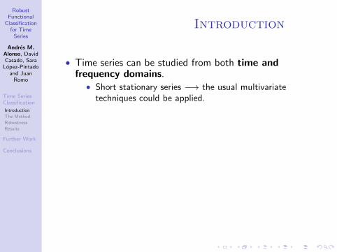
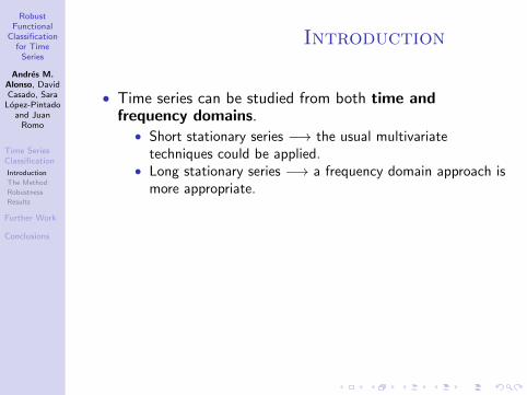
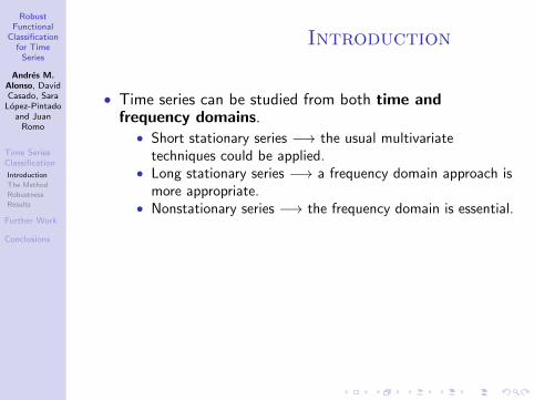
• Time series can be studied from both time andfrequency domains.
• Short stationary series −→ the usual multivariatetechniques could be applied.
• Long stationary series −→ a frequency domain approach ismore appropriate.
• Nonstationary series −→ the frequency domain is essential.
• There are several works on classification methods fromboth domains.
• Most authors have studied the classification of stationarytime series.
RobustFunctional
Classificationfor Time
Series
Andres M.Alonso, DavidCasado, Sara
Lopez-Pintadoand Juan
Romo
Time SeriesClassification
Introduction
The Method
Robustness
Results
Further Work
Conclusions
Introduction
• Time series can be studied from both time andfrequency domains.• Short stationary series −→ the usual multivariate
techniques could be applied.
• Long stationary series −→ a frequency domain approach ismore appropriate.
• Nonstationary series −→ the frequency domain is essential.
• There are several works on classification methods fromboth domains.
• Most authors have studied the classification of stationarytime series.
RobustFunctional
Classificationfor Time
Series
Andres M.Alonso, DavidCasado, Sara
Lopez-Pintadoand Juan
Romo
Time SeriesClassification
Introduction
The Method
Robustness
Results
Further Work
Conclusions
Introduction
• Time series can be studied from both time andfrequency domains.• Short stationary series −→ the usual multivariate
techniques could be applied.• Long stationary series −→ a frequency domain approach is
more appropriate.
• Nonstationary series −→ the frequency domain is essential.
• There are several works on classification methods fromboth domains.
• Most authors have studied the classification of stationarytime series.
RobustFunctional
Classificationfor Time
Series
Andres M.Alonso, DavidCasado, Sara
Lopez-Pintadoand Juan
Romo
Time SeriesClassification
Introduction
The Method
Robustness
Results
Further Work
Conclusions
Introduction
• Time series can be studied from both time andfrequency domains.• Short stationary series −→ the usual multivariate
techniques could be applied.• Long stationary series −→ a frequency domain approach is
more appropriate.• Nonstationary series −→ the frequency domain is essential.
• There are several works on classification methods fromboth domains.
• Most authors have studied the classification of stationarytime series.

RobustFunctional
Classificationfor Time
Series
Andres M.Alonso, DavidCasado, Sara
Lopez-Pintadoand Juan
Romo
Time SeriesClassification
Introduction
The Method
Robustness
Results
Further Work
Conclusions
Introduction
Classification of Stationary Series
• Pulli (1996) considers the ratio of spectra.
• Kakizawa, Shumway and Taniguchi (1998) discriminatemultivariate time series with the Kullback-Leibler’s and theChernoff’s information measures.
Classification of Nonstationary Series
• Ombao et al. (2001) introduce the SLEX spectrum for anonstationary random process.
• Caiado et al. (2006): define a measure, based on theperiodogram, for both clustering and classifying stationaryand nonstationary time series.

RobustFunctional
Classificationfor Time
Series
Andres M.Alonso, DavidCasado, Sara
Lopez-Pintadoand Juan
Romo
Time SeriesClassification
Introduction
The Method
Robustness
Results
Further Work
Conclusions
Introduction
Models for Nonstationary Series
• Priestley (1965) introduces the concept of a Cramerrepresentation with time-varying transfer function.
Xt =
∫ +π
−πe iλtAt(λ)dξ(λ)
• Dahlhaus (1996) establishes an asymptotic framework forlocally stationary processes.
Xt,T = µ( t
T
)+
∫ +π
−πe iλtA0
t,T (λ)dξ(λ)
RobustFunctional
Classificationfor Time
Series
Andres M.Alonso, DavidCasado, Sara
Lopez-Pintadoand Juan
Romo
Time SeriesClassification
Introduction
The Method
Robustness
Results
Further Work
Conclusions
Context
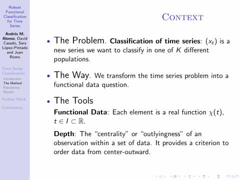
• The Problem. Classification of time series: (xt) is anew series we want to classify in one of K differentpopulations.
• The Way. We transform the time series problem into afunctional data question.
• The ToolsFunctional Data: Each element is a real function χ(t),t ∈ I ⊂ R.
Depth: The “centrality” or “outlyingness” of anobservation within a set of data. It provides a criterion toorder data from center-outward.
RobustFunctional
Classificationfor Time
Series
Andres M.Alonso, DavidCasado, Sara
Lopez-Pintadoand Juan
Romo
Time SeriesClassification
Introduction
The Method
Robustness
Results
Further Work
Conclusions
Context
• The Problem. Classification of time series: (xt) is anew series we want to classify in one of K differentpopulations.
• The Way. We transform the time series problem into afunctional data question.
• The ToolsFunctional Data: Each element is a real function χ(t),t ∈ I ⊂ R.
Depth: The “centrality” or “outlyingness” of anobservation within a set of data. It provides a criterion toorder data from center-outward.

RobustFunctional
Classificationfor Time
Series
Andres M.Alonso, DavidCasado, Sara
Lopez-Pintadoand Juan
Romo
Time SeriesClassification
Introduction
The Method
Robustness
Results
Further Work
Conclusions
Functional Data
Let (xt) = (x1, . . . , xT ) be a time series, the periodogram andits cumulative version, the integrated periodogram, are:
IT (λj) =1
2πT
∣∣∣∣∣T∑
t=+1
xte−itλj
∣∣∣∣∣2
, λj ∈ S
FT (λj) =1
cT
j∑i=1
IT (λi ), λi ∈ S, λj ∈ S
where
S ={λj = 2πj
T , j = −[T−1
2
], . . . ,−1, 0,+1, . . . ,+
[T2
]}is the Fourier set of frequencies.
RobustFunctional
Classificationfor Time
Series
Andres M.Alonso, DavidCasado, Sara
Lopez-Pintadoand Juan
Romo
Time SeriesClassification
Introduction
The Method
Robustness
Results
Further Work
Conclusions
Classification Criterion
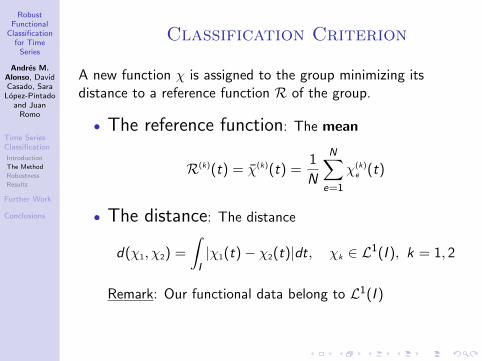
A new function χ is assigned to the group minimizing itsdistance to a reference function R of the group.
• The reference function: The mean
R(k)(t) = χ(k)(t) =1
N
N∑e=1
χ(k)e (t)
• The distance: The distance
d(χ1, χ2) =
∫I|χ1(t)− χ2(t)|dt, χk ∈ L1(I ), k = 1, 2
Remark: Our functional data belong to L1(I )
RobustFunctional
Classificationfor Time
Series
Andres M.Alonso, DavidCasado, Sara
Lopez-Pintadoand Juan
Romo
Time SeriesClassification
Introduction
The Method
Robustness
Results
Further Work
Conclusions
Depth
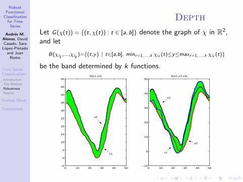
Let G(χ(t)) = {(t, χ(t)) : t ∈ [a, b]} denote the graph of χ in R2,and let
B(χi1,...,χik
)={(t,y) | t∈[a,b], minr=1,...,k χir (t)≤y≤maxr=1,...,k χir (t)}
be the band determined by k functions.
0 10 20 30 40 50−5
0
5
10
15
20
25
30
35
40
45
50B(x1,x2)
0 10 20 30 40 50−10
0
10
20
30
40
50B(x1,x2,x3)
x1
x2
x1
x2
x3
RobustFunctional
Classificationfor Time
Series
Andres M.Alonso, DavidCasado, Sara
Lopez-Pintadoand Juan
Romo
Time SeriesClassification
Introduction
The Method
Robustness
Results
Further Work
Conclusions
Depth
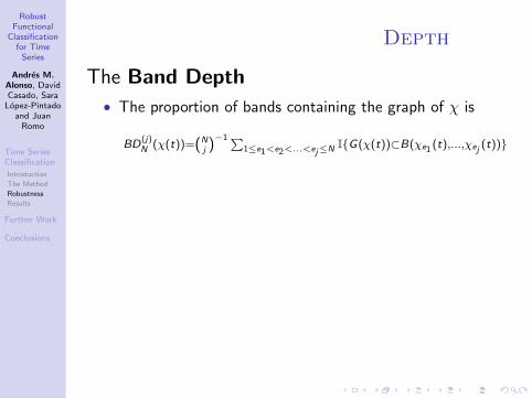
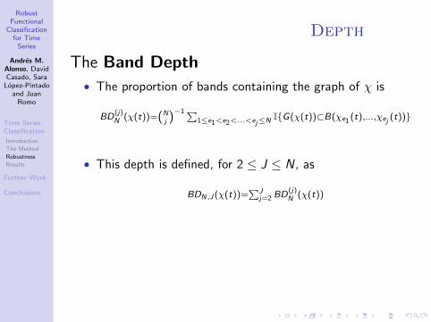
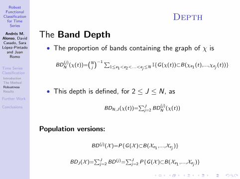
The Band Depth
• The proportion of bands containing the graph of χ is
BD(j)N (χ(t))=(Nj )
−1∑1≤e1<e2<...<ej≤N I{G(χ(t))⊂B(χe1 (t),...,χej
(t))}
• This depth is defined, for 2 ≤ J ≤ N, as
BDN,J(χ(t))=∑J
j=2 BD(j)N (χ(t))
Population versions:
BD(j)(X )=P{G(X )⊂B(Xe1 ,...,Xej)}
BDJ(X )=∑J
j=2 BD(j)=
∑Jj=2 P{G(X )⊂B(Xe1 ,...,Xej
)}
RobustFunctional
Classificationfor Time
Series
Andres M.Alonso, DavidCasado, Sara
Lopez-Pintadoand Juan
Romo
Time SeriesClassification
Introduction
The Method
Robustness
Results
Further Work
Conclusions
Depth
The Band Depth
• The proportion of bands containing the graph of χ is
BD(j)N (χ(t))=(Nj )
−1∑1≤e1<e2<...<ej≤N I{G(χ(t))⊂B(χe1 (t),...,χej
(t))}
• This depth is defined, for 2 ≤ J ≤ N, as
BDN,J(χ(t))=∑J
j=2 BD(j)N (χ(t))
Population versions:
BD(j)(X )=P{G(X )⊂B(Xe1 ,...,Xej)}
BDJ(X )=∑J
j=2 BD(j)=
∑Jj=2 P{G(X )⊂B(Xe1 ,...,Xej
)}
RobustFunctional
Classificationfor Time
Series
Andres M.Alonso, DavidCasado, Sara
Lopez-Pintadoand Juan
Romo
Time SeriesClassification
Introduction
The Method
Robustness
Results
Further Work
Conclusions
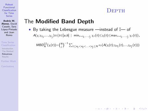
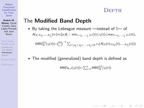
Depth
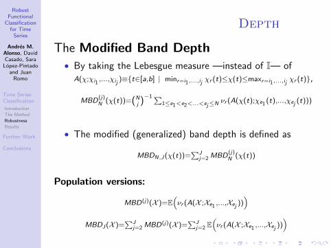
The Modified Band Depth• By taking the Lebesgue measure —instead of I— of
A(χ;χi1,...,χij
)≡{t∈[a,b] | minr=i1,...,ijχr (t)≤χ(t)≤maxr=i1,...,ij
χr (t)},
MBD(j)N (χ(t))=(Nj )
−1∑1≤e1<e2<...<ej≤N νr (A(χ(t);χe1 (t),...,χej
(t)))
• The modified (generalized) band depth is defined as
MBDN,J(χ(t))=∑J
j=2 MBD(j)N (χ(t))
Population versions:
MBD(j)(X )=E(νr (A(X ;Xe1 ,...,Xej
)))
MBDJ(X )=∑J
j=2 MBD(j)(X )=∑J
j=2 E(νr (A(X ;Xe1 ,...,Xej
)))
RobustFunctional
Classificationfor Time
Series
Andres M.Alonso, DavidCasado, Sara
Lopez-Pintadoand Juan
Romo
Time SeriesClassification
Introduction
The Method
Robustness
Results
Further Work
Conclusions
Depth
The Modified Band Depth• By taking the Lebesgue measure —instead of I— of
A(χ;χi1,...,χij
)≡{t∈[a,b] | minr=i1,...,ijχr (t)≤χ(t)≤maxr=i1,...,ij
χr (t)},
MBD(j)N (χ(t))=(Nj )
−1∑1≤e1<e2<...<ej≤N νr (A(χ(t);χe1 (t),...,χej
(t)))
• The modified (generalized) band depth is defined as
MBDN,J(χ(t))=∑J
j=2 MBD(j)N (χ(t))
Population versions:
MBD(j)(X )=E(νr (A(X ;Xe1 ,...,Xej
)))
MBDJ(X )=∑J
j=2 MBD(j)(X )=∑J
j=2 E(νr (A(X ;Xe1 ,...,Xej
)))
RobustFunctional
Classificationfor Time
Series
Andres M.Alonso, DavidCasado, Sara
Lopez-Pintadoand Juan
Romo
Time SeriesClassification
Introduction
The Method
Robustness
Results
Further Work
Conclusions
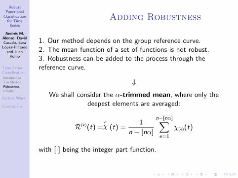
Adding Robustness
1. Our method depends on the group reference curve.2. The mean function of a set of functions is not robust.3. Robustness can be added to the process through thereference curve.
⇓
We shall consider the α-trimmed mean, where only thedeepest elements are averaged:
R(k)(t) =α
χ (t) =1
n − [nα]
n−[nα]∑e=1
χ(e)(t)
with [·] being the integer part function.
RobustFunctional
Classificationfor Time
Series
Andres M.Alonso, DavidCasado, Sara
Lopez-Pintadoand Juan
Romo
Time SeriesClassification
Introduction
The Method
Robustness
Results
Further Work
Conclusions
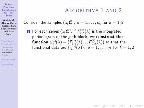
Algorithms 1 and 2
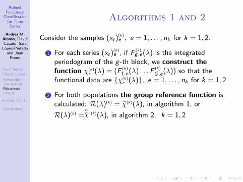
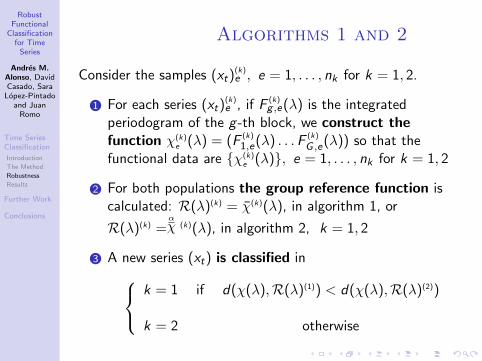
Consider the samples (xt)(k)e , e = 1, . . . , nk for k = 1, 2.
1 For each series (xt)(k)e , if F (k)
g ,e(λ) is the integratedperiodogram of the g -th block, we construct thefunction χ(k)
e (λ) = (F (k)
1,e(λ) . . .F (k)
G ,e(λ)) so that thefunctional data are {χ(k)
e (λ)}, e = 1, . . . , nk for k = 1, 2
2 For both populations the group reference function iscalculated: R(λ)(k) = χ(k)(λ), in algorithm 1, or
R(λ)(k) =α
χ (k)(λ), in algorithm 2, k = 1, 2
3 A new series (xt) is classified ink = 1 if d(χ(λ),R(λ)(1)) < d(χ(λ),R(λ)(2))
k = 2 otherwise
RobustFunctional
Classificationfor Time
Series
Andres M.Alonso, DavidCasado, Sara
Lopez-Pintadoand Juan
Romo
Time SeriesClassification
Introduction
The Method
Robustness
Results
Further Work
Conclusions
Algorithms 1 and 2
Consider the samples (xt)(k)e , e = 1, . . . , nk for k = 1, 2.
1 For each series (xt)(k)e , if F (k)
g ,e(λ) is the integratedperiodogram of the g -th block, we construct thefunction χ(k)
e (λ) = (F (k)
1,e(λ) . . .F (k)
G ,e(λ)) so that thefunctional data are {χ(k)
e (λ)}, e = 1, . . . , nk for k = 1, 2
2 For both populations the group reference function iscalculated: R(λ)(k) = χ(k)(λ), in algorithm 1, or
R(λ)(k) =α
χ (k)(λ), in algorithm 2, k = 1, 2
3 A new series (xt) is classified ink = 1 if d(χ(λ),R(λ)(1)) < d(χ(λ),R(λ)(2))
k = 2 otherwise
RobustFunctional
Classificationfor Time
Series
Andres M.Alonso, DavidCasado, Sara
Lopez-Pintadoand Juan
Romo
Time SeriesClassification
Introduction
The Method
Robustness
Results
Further Work
Conclusions
The SLEXbC Method
Using the SLEX (smooth localized complex exponential) modelof a nonstationary random process, Huang et al. (2004)propose a classification method (SLEXbC).
We compare our algorithms with this method.
How SLEXbC works
1 It finds a basis from the SLEX library that can best detectthe differences.
2 It assigns to the class minimizing the Kullback-Leiblerdivergence between the SLEX spectra.
RobustFunctional
Classificationfor Time
Series
Andres M.Alonso, DavidCasado, Sara
Lopez-Pintadoand Juan
Romo
Time SeriesClassification
Introduction
The Method
Robustness
Results
Further Work
Conclusions
Simulations
Let (xt)(k)e be the e-th series of the k-th population; let εt ∼ N(0, 1) be
Gaussian noise.
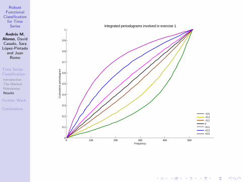
Simulation 1. Series are stationary
X (1)
t = φX (1)
t−1 + ε(1)
t t = 1, . . . ,T
X (2)
t = ε(2)
t t = 1, . . . ,T
Training data sets sizes: n = 8 series of length T = 1024.Testing data sets sizes: n = 10 series of length T = 1024.Six comparisons: Values φ = −0.5, −0.3, −0.1, +0.1, +0.3 and +0.5.
Runs: 1000.
RobustFunctional
Classificationfor Time
Series
Andres M.Alonso, DavidCasado, Sara
Lopez-Pintadoand Juan
Romo
Time SeriesClassification
Introduction
The Method
Robustness
Results
Further Work
Conclusions
Simulations
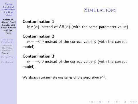
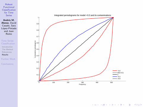
Contamination 1MA(φ) instead of AR(φ) (with the same parameter value).
Contamination 2φ = −0.9 instead of the correct value φ (with the correct
model).
Contamination 3φ = +0.9 instead of the correct value φ (with the correct
model).
We always contaminate one series of the population P (1).
RobustFunctional
Classificationfor Time
Series
Andres M.Alonso, DavidCasado, Sara
Lopez-Pintadoand Juan
Romo
Time SeriesClassification
Introduction
The Method
Robustness
Results
Further Work
Conclusions
0 100 200 300 400 5000
0.1
0.2
0.3
0.4
0.5
0.6
0.7
0.8
0.9
1
Frequency
Cu
mu
lativ
e p
erio
do
gra
m
Integrated periodograms involved in exercise 1
−0.5−0.3−0.10+0.1+0.3+0.5
RobustFunctional
Classificationfor Time
Series
Andres M.Alonso, DavidCasado, Sara
Lopez-Pintadoand Juan
Romo
Time SeriesClassification
Introduction
The Method
Robustness
Results
Further Work
Conclusions
0 100 200 300 400 5000
0.1
0.2
0.3
0.4
0.5
0.6
0.7
0.8
0.9
1
Frequency
Cu
mu
lativ
e p
erio
do
gra
m
Integrated periodograms for model +0.3 and its contaminations
−0.9MA(+0.3)0+0.3+0.9
RobustFunctional
Classificationfor Time
Series
Andres M.Alonso, DavidCasado, Sara
Lopez-Pintadoand Juan
Romo
Time SeriesClassification
Introduction
The Method
Robustness
Results
Further Work
Conclusions
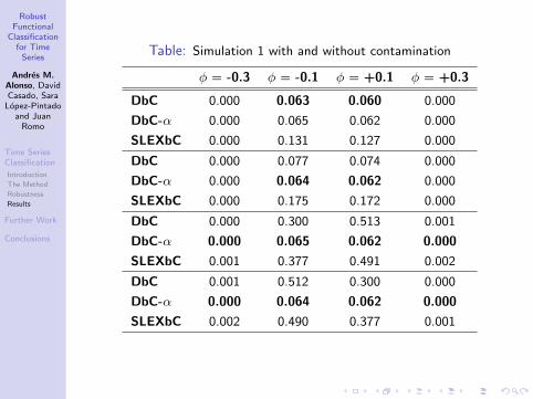
Table: Simulation 1 with and without contamination
φ = -0.3 φ = -0.1 φ = +0.1 φ = +0.3
DbC 0.000 0.063 0.060 0.000
DbC-α 0.000 0.065 0.062 0.000
SLEXbC 0.000 0.131 0.127 0.000
DbC 0.000 0.077 0.074 0.000
DbC-α 0.000 0.064 0.062 0.000
SLEXbC 0.000 0.175 0.172 0.000
DbC 0.000 0.300 0.513 0.001
DbC-α 0.000 0.065 0.062 0.000
SLEXbC 0.001 0.377 0.491 0.002
DbC 0.001 0.512 0.300 0.000
DbC-α 0.000 0.064 0.062 0.000
SLEXbC 0.002 0.490 0.377 0.001

RobustFunctional
Classificationfor Time
Series
Andres M.Alonso, DavidCasado, Sara
Lopez-Pintadoand Juan
Romo
Time SeriesClassification
Introduction
The Method
Robustness
Results
Further Work
Conclusions
DbC DbC−a SLEXbC DbC DbC−a SLEXbC DbC DbC−a SLEXbC DbC DbC−a SLEXbC
0
0.1
0.2
0.3
0.4
0.5
0.6
0.7
Va
lue
s
−0.1 versus 0
RobustFunctional
Classificationfor Time
Series
Andres M.Alonso, DavidCasado, Sara
Lopez-Pintadoand Juan
Romo
Time SeriesClassification
Introduction
The Method
Robustness
Results
Further Work
Conclusions
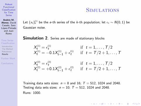
Simulations
Let (xt)(k)e be the e-th series of the k-th population; let εt ∼ N(0, 1) be
Gaussian noise.
Simulation 2. Series are made of stationary blocks
X (1)
t = ε(1)
t if t = 1, . . . ,T/2
X (1)
t = −0.1X (1)
t−1 + ε(1)
t if t = T/2 + 1, . . . ,T
X (2)
t = ε(2)
t if t = 1, . . . ,T/2
X (2)
t = +0.1X (2)
t−1 + ε(2)
t if t = T/2 + 1, . . . ,T
Training data sets sizes: n = 8 and 16; T = 512, 1024 and 2048.Testing data sets sizes: n = 10; T = 512, 1024 and 2048.
Runs: 1000.

RobustFunctional
Classificationfor Time
Series
Andres M.Alonso, DavidCasado, Sara
Lopez-Pintadoand Juan
Romo
Time SeriesClassification
Introduction
The Method
Robustness
Results
Further Work
Conclusions
Simulations
Contamination 1MA(φ) instead of AR(φ) (with the same parameter value).
Contamination 2φ = −0.9 instead of the correct value φ (with the correct
model).
Contamination 3φ = +0.9 instead of the correct value φ (with the correct
model).
We always contaminate one series of the population P (1).
RobustFunctional
Classificationfor Time
Series
Andres M.Alonso, DavidCasado, Sara
Lopez-Pintadoand Juan
Romo
Time SeriesClassification
Introduction
The Method
Robustness
Results
Further Work
Conclusions
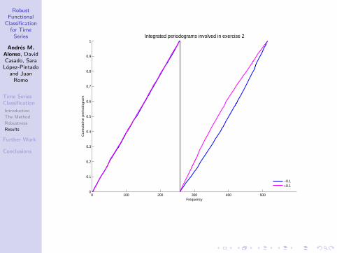
0 100 200 300 400 5000
0.1
0.2
0.3
0.4
0.5
0.6
0.7
0.8
0.9
1Integrated periodograms involved in exercise 2
Frequency
Cu
mu
lativ
e p
erio
do
gra
m
−0.1+0.1
RobustFunctional
Classificationfor Time
Series
Andres M.Alonso, DavidCasado, Sara
Lopez-Pintadoand Juan
Romo
Time SeriesClassification
Introduction
The Method
Robustness
Results
Further Work
Conclusions
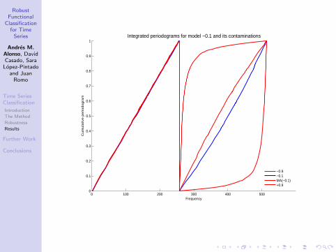
0 100 200 300 400 5000
0.1
0.2
0.3
0.4
0.5
0.6
0.7
0.8
0.9
1Integrated periodograms for model −0.1 and its contaminations
Frequency
Cu
mu
lativ
e p
erio
do
gra
m
−0.9−0.1MA(−0.1)+0.9
RobustFunctional
Classificationfor Time
Series
Andres M.Alonso, DavidCasado, Sara
Lopez-Pintadoand Juan
Romo
Time SeriesClassification
Introduction
The Method
Robustness
Results
Further Work
Conclusions
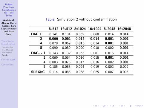
Table: Simulation 2 without contamination
8x512 16x512 8x1024 16x1024 8x2048 16x2048
DbC 1 0.141 0.131 0.062 0.060 0.014 0.014
2 0.066 0.061 0.015 0.014 0.001 0.0014 0.078 0.069 0.015 0.014 0.001 0.0018 0.090 0.080 0.020 0.018 0.002 0.001
DbC-α 1 0.143 0.132 0.063 0.061 0.015 0.014
2 0.069 0.064 0.016 0.015 0.001 0.0014 0.083 0.073 0.017 0.016 0.002 0.0018 0.105 0.088 0.024 0.019 0.002 0.002
SLEXbC 0.114 0.086 0.038 0.025 0.007 0.003
RobustFunctional
Classificationfor Time
Series
Andres M.Alonso, DavidCasado, Sara
Lopez-Pintadoand Juan
Romo
Time SeriesClassification
Introduction
The Method
Robustness
Results
Further Work
Conclusions
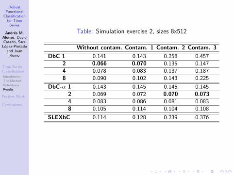
Table: Simulation exercise 2, sizes 8x512
Without contam. Contam. 1 Contam. 2 Contam. 3
DbC 1 0.141 0.143 0.258 0.457
2 0.066 0.070 0.135 0.147
4 0.078 0.083 0.137 0.187
8 0.090 0.102 0.143 0.225
DbC-α 1 0.143 0.145 0.145 0.145
2 0.069 0.072 0.070 0.0734 0.083 0.086 0.081 0.083
8 0.105 0.114 0.104 0.108
SLEXbC 0.114 0.128 0.239 0.376
RobustFunctional
Classificationfor Time
Series
Andres M.Alonso, DavidCasado, Sara
Lopez-Pintadoand Juan
Romo
Time SeriesClassification
Introduction
The Method
Robustness
Results
Further Work
Conclusions
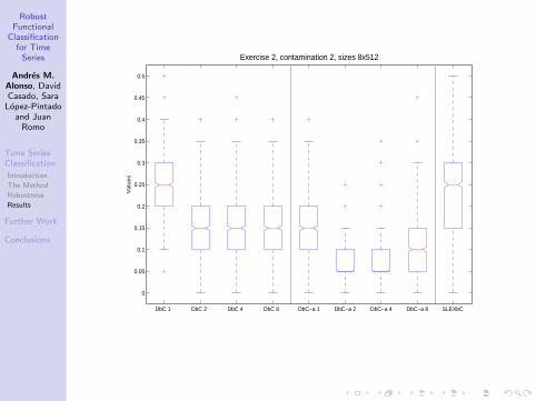
DbC 1 DbC 2 DbC 4 DbC 8 DbC−a 1 DbC−a 2 DbC−a 4 DbC−a 8 SLEXbC
0
0.05
0.1
0.15
0.2
0.25
0.3
0.35
0.4
0.45
0.5
Va
lue
s
Exercise 2, contamination 2, sizes 8x512

RobustFunctional
Classificationfor Time
Series
Andres M.Alonso, DavidCasado, Sara
Lopez-Pintadoand Juan
Romo
Time SeriesClassification
Introduction
The Method
Robustness
Results
Further Work
Conclusions
Simulations
Let (xt)(k)e be the e-th series of the k-th population; let εt ∼ N(0, 1) be
Gaussian noise.
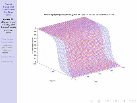
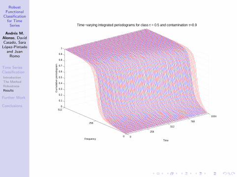
Simulation 3. Series are not stationary
If at;τ = 0.8 · [1− τ cos(πt/1024)], then
X (1)
t = at;0.5X(1)
t−1 − 0.81X (1)
t−2 + ε(1)
t t = 1, . . . ,T
X (2)
t = at;τX(2)
t−1 − 0.81X (2)
t−2 + ε(2)
t t = 1, . . . ,T
Training and testing data sets sizes: n = 10; T = 1024.Three comparisons: τ values 0.4, 0.3 and 0.2.Runs: 1000.
RobustFunctional
Classificationfor Time
Series
Andres M.Alonso, DavidCasado, Sara
Lopez-Pintadoand Juan
Romo
Time SeriesClassification
Introduction
The Method
Robustness
Results
Further Work
Conclusions
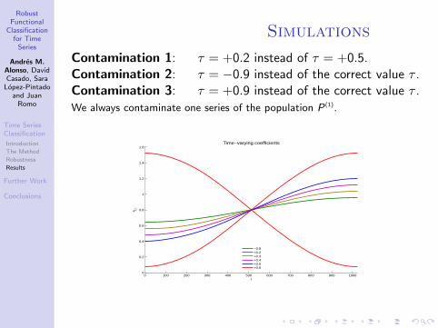
Simulations
Contamination 1: τ = +0.2 instead of τ = +0.5.Contamination 2: τ = −0.9 instead of the correct value τ .Contamination 3: τ = +0.9 instead of the correct value τ .We always contaminate one series of the population P (1).
0 100 200 300 400 500 600 700 800 900 10000
0.2
0.4
0.6
0.8
1
1.2
1.4
1.6
t
a t;τ
Time−varying coefficients
−0.9+0.2+0.3+0.4+0.5+0.9
RobustFunctional
Classificationfor Time
Series
Andres M.Alonso, DavidCasado, Sara
Lopez-Pintadoand Juan
Romo
Time SeriesClassification
Introduction
The Method
Robustness
Results
Further Work
Conclusions
0
256
512
768
1024
0
256
5120
0.1
0.2
0.3
0.4
0.5
0.6
0.7
0.8
0.9
1
Time
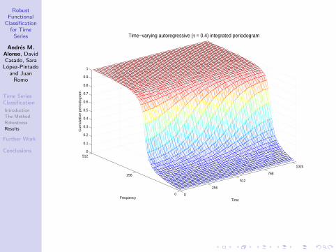
Time−varying autoregressive (τ = 0.4) integrated periodogram
Frequency
Cu
mu
lativ
e p
erio
do
gra
m
RobustFunctional
Classificationfor Time
Series
Andres M.Alonso, DavidCasado, Sara
Lopez-Pintadoand Juan
Romo
Time SeriesClassification
Introduction
The Method
Robustness
Results
Further Work
Conclusions
0
256
512
768
1024
0
256
5120
0.1
0.2
0.3
0.4
0.5
0.6
0.7
0.8
0.9
1
Time
Time−varying integrated periodograms for class τ = 0.5 and contamination τ=−0.9
Frequency
Cu
mu
lativ
e p
erio
do
gra
m
RobustFunctional
Classificationfor Time
Series
Andres M.Alonso, DavidCasado, Sara
Lopez-Pintadoand Juan
Romo
Time SeriesClassification
Introduction
The Method
Robustness
Results
Further Work
Conclusions
0
256
512
768
1024
0
256
5120
0.1
0.2
0.3
0.4
0.5
0.6
0.7
0.8
0.9
1
Time
Time−varying integrated periodograms for class τ = 0.5 and contamination τ=0.9
Frequency
Cu
mu
lativ
e p
erio
do
gra
m
RobustFunctional
Classificationfor Time
Series
Andres M.Alonso, DavidCasado, Sara
Lopez-Pintadoand Juan
Romo
Time SeriesClassification
Introduction
The Method
Robustness
Results
Further Work
Conclusions
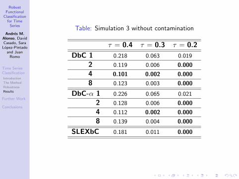
Table: Simulation 3 without contamination
τ = 0.4 τ = 0.3 τ = 0.2
DbC 1 0.218 0.063 0.019
2 0.119 0.006 0.000
4 0.101 0.002 0.000
8 0.123 0.003 0.000
DbC-α 1 0.226 0.065 0.021
2 0.128 0.006 0.000
4 0.112 0.002 0.000
8 0.139 0.004 0.000
SLEXbC 0.181 0.011 0.000
RobustFunctional
Classificationfor Time
Series
Andres M.Alonso, DavidCasado, Sara
Lopez-Pintadoand Juan
Romo
Time SeriesClassification
Introduction
The Method
Robustness
Results
Further Work
Conclusions
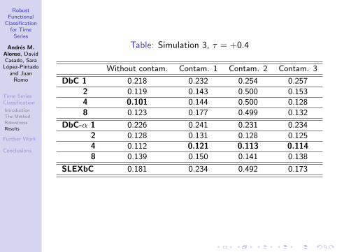
Table: Simulation 3, τ = +0.4
Without contam. Contam. 1 Contam. 2 Contam. 3
DbC 1 0.218 0.232 0.254 0.257
2 0.119 0.143 0.500 0.153
4 0.101 0.144 0.500 0.128
8 0.123 0.177 0.499 0.132
DbC-α 1 0.226 0.241 0.231 0.234
2 0.128 0.131 0.128 0.125
4 0.112 0.121 0.113 0.1148 0.139 0.150 0.141 0.138
SLEXbC 0.181 0.234 0.492 0.173
RobustFunctional
Classificationfor Time
Series
Andres M.Alonso, DavidCasado, Sara
Lopez-Pintadoand Juan
Romo
Time SeriesClassification
Introduction
The Method
Robustness
Results
Further Work
Conclusions
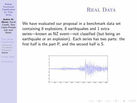
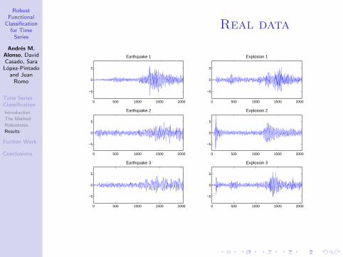
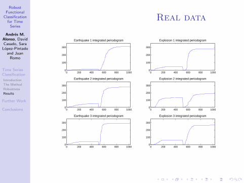
Real Data
We have evaluated our proposal in a benchmark data setcontaining 8 explosions, 8 earthquakes and 1 extraseries—known as NZ event—not classified (but being anearthquake or an explosion). Each series has two parts: thefirst half is the part P, and the second half is S.
0 200 400 600 800 1000 1200 1400 1600 1800 2000−8
−6
−4
−2
0
2
4
6
8
RobustFunctional
Classificationfor Time
Series
Andres M.Alonso, DavidCasado, Sara
Lopez-Pintadoand Juan
Romo
Time SeriesClassification
Introduction
The Method
Robustness
Results
Further Work
Conclusions
Real data
0 500 1000 1500 2000
−5
0
5
Earthquake 1
0 500 1000 1500 2000
−5
0
5
Explosion 1
0 500 1000 1500 2000
−5
0
5
Earthquake 2
0 500 1000 1500 2000
−5
0
5
Explosion 2
0 500 1000 1500 2000
−5
0
5
Earthquake 3
0 500 1000 1500 2000
−5
0
5
Explosion 3
RobustFunctional
Classificationfor Time
Series
Andres M.Alonso, DavidCasado, Sara
Lopez-Pintadoand Juan
Romo
Time SeriesClassification
Introduction
The Method
Robustness
Results
Further Work
Conclusions
Real data
0 200 400 600 800 10000
100
200
300
Earthquake 1 integrated periodogram
0 200 400 600 800 10000
100
200
300
Explosion 1 integrated periodogram
0 200 400 600 800 10000
100
200
300
Earthquake 2 integrated periodogram
0 200 400 600 800 10000
100
200
300
Explosion 2 integrated periodogram
0 200 400 600 800 10000
100
200
300
Earthquake 3 integrated periodogram
0 200 400 600 800 10000
100
200
300
Explosion 3 integrated periodogram
RobustFunctional
Classificationfor Time
Series
Andres M.Alonso, DavidCasado, Sara
Lopez-Pintadoand Juan
Romo
Time SeriesClassification
Introduction
The Method
Robustness
Results
Further Work
Conclusions
Real Data
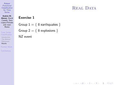
Exercise 1
Group 1 = { 8 earthquakes }
Group 2 = { 8 explosions }
NZ event
• Applying leave-one-out cross validation, both of ouralgorithms misclassify only the first series of thegroup 2 (explosions).
• Respecting the NZ event, both algorithms agree onassigning it to the explosions group, as, for example,Kakizawa et al. (1998) and Huang et al. (2004).
RobustFunctional
Classificationfor Time
Series
Andres M.Alonso, DavidCasado, Sara
Lopez-Pintadoand Juan
Romo
Time SeriesClassification
Introduction
The Method
Robustness
Results
Further Work
Conclusions
Real Data
Exercise 1
Group 1 = { 8 earthquakes }
Group 2 = { 8 explosions }
NZ event
• Applying leave-one-out cross validation, both of ouralgorithms misclassify only the first series of thegroup 2 (explosions).
• Respecting the NZ event, both algorithms agree onassigning it to the explosions group, as, for example,Kakizawa et al. (1998) and Huang et al. (2004).

RobustFunctional
Classificationfor Time
Series
Andres M.Alonso, DavidCasado, Sara
Lopez-Pintadoand Juan
Romo
Time SeriesClassification
Introduction
The Method
Robustness
Results
Further Work
Conclusions
Real Data
Exercise 2
Group 1 = { 8 earthquakes + NZ event }
Group 2 = { 8 explosions }
We can consider that a atypical observation is presented in group 1.
• In this situation, algorithm 1 misclassifies the first andthird elements of group 2 (explosions), not only the first.
• But again algorithm 2 misclassifies only the firstseries of group 2. This illustrates the robustness of oursecond algorithm.

RobustFunctional
Classificationfor Time
Series
Andres M.Alonso, DavidCasado, Sara
Lopez-Pintadoand Juan
Romo
Time SeriesClassification
Introduction
The Method
Robustness
Results
Further Work
Conclusions
Real Data
Results
Table: Misclassified series
Exercise 1 Exercise 2DbC Explosion 1 Explosions 1 and 3DbC-α Explosion 1 Explosions 1

RobustFunctional
Classificationfor Time
Series
Andres M.Alonso, DavidCasado, Sara
Lopez-Pintadoand Juan
Romo
Time SeriesClassification
Introduction
The Method
Robustness
Results
Further Work
Conclusions
Further Work
RobustFunctional
Classificationfor Time
Series
Andres M.Alonso, DavidCasado, Sara
Lopez-Pintadoand Juan
Romo
Time SeriesClassification
Introduction
The Method
Robustness
Results
Further Work
Conclusions
Time Series Method
1 K -group classification can be dealt with
k = argmin{1,...,K}
{d(χ(λ),R(k)(λ))
}.
2 Clustering of time series, by tackling the associatedfunctional data problem in the frequency domain.
3 Other different definitions of depth can be considered, forexample: Fraiman and Muniz (2001), Cuevas et al.(2007).

RobustFunctional
Classificationfor Time
Series
Andres M.Alonso, DavidCasado, Sara
Lopez-Pintadoand Juan
Romo
Time SeriesClassification
Introduction
The Method
Robustness
Results
Further Work
Conclusions
Conclusions
RobustFunctional
Classificationfor Time
Series
Andres M.Alonso, DavidCasado, Sara
Lopez-Pintadoand Juan
Romo
Time SeriesClassification
Introduction
The Method
Robustness
Results
Further Work
Conclusions
Time Series Method
• We define a new time series classification method basedon the integrated periodogram.
• The method can also work with nonstationary series bysplitting them into blocks and computing the integratedperiodogram of each block.
• By substituting the mean by the α-trimmed mean themethod becomes robust.
• The method has shown good behavior in a wide range ofsimulation exercises and with real data, improving onexisting methods.
• It suggests that the integrated periodogram containsuseful information to classify time series.

RobustFunctional
Classificationfor Time
Series
Andres M.Alonso, DavidCasado, Sara
Lopez-Pintadoand Juan
Romo
Time SeriesClassification
Introduction
The Method
Robustness
Results
Further Work
Conclusions
References
Caiado, J., N. Crato and D. Pena (2006). A Periodogram-Based Metricfor Time Series Classification. Computational Statistics &Data Analysis. 50, 2668–2684.
Dahlhaus, R. (1996). Asymptotic Statistical Inference for NonstationaryProcesses with Evolutionary Spectra. Athens Conferenceon Applied Probability and Time Series Analysis, Vol. 2(P.M. Robinson and M. Rosenblatt, eds.). Lecture Notesin Statist. 115 145–159. Springer- -Verlag. 6, 171–191.
Huang, H., H. Ombao and D.S. Stoffer (2004). Discrimination andClassification of Nonstationary Time Series Using theSLEX Model. Journal of the American StatisticalAssociation. 99 (467), 763–774.
Kakizawa, Y., R.H. Shumway and M. Taniguchi (1998). Discriminationand Clustering for Multivariate Time Series. Journal of theAmerican Statistical Association. 93 (441), 328–340.
RobustFunctional
Classificationfor Time
Series
Andres M.Alonso, DavidCasado, Sara
Lopez-Pintadoand Juan
Romo
Time SeriesClassification
Introduction
The Method
Robustness
Results
Further Work
Conclusions
References
Lopez-Pintado, S., and J. Romo (2009). On the Concept of Depth forFunctional Data. Journal of the American StatisticalAssociation. 93 (441), 328–340.
Ombao, H.C., J.A. Raz, R. von Sachs and B.A. Malow (2001). AutomaticStatistical Analysis of Bivariate Nonstationary Time Series.Journal of the American Statistical Association. 104 (486),704–717.
Pulli, J. (1996). Extracting and processing signal parameters forregional seismic event identification, in Monitoring aComprehensive Test Ban Treaty.
Priestley, M. (1965). Evolutionary Spectra and Non-StationaryProcesses. Journal of the Royal Statistical Society. SeriesB, 27 (2), 204–237. NATO Advanced Study InstituteSeries. Vol. 303, Kluwer Press, 743–754 (eds E. Husebyeand A. Dainty).