Detrending the Business Cycles:Hodrick-Prescott and Baxter-King Filters

Bahar Dadashova

Pro¤esor: Regina KaiserIntroduction to Time Series

Master O�cial en Economia de la Empresa y Metodos Cuantitativos,Universidad Carlos III de Madrid

1

Contents

1. Introduction

2. Detrending the business cycles

(a) Hodrick-Prescott �lter

(b) Baxter-King �lter

3. Problems Associated with Hodrick-Prescott �lter

(a) End Point Estimation

(b) Spurious E¤ect

4. Summary

5. Literature

6. Appendix

(a) MATLAB Routines

(b) Graphs

2

Detrending the Business Cycles:Hodrick-Prescott andBaxter-King Filters

Abstract

The purpose of this paper is to see comparative analsis of two �lters,Hodrick-Prescott and Baxter-King �lters. The review of the literature onthis topic show that the applicaion of the Hodrick-Prescott �lter to thetime series would produce spurious e¤ect as well as poor approximationof the data near the end points is observed. Alternative �lter which wasproposed by Baxter- King (1995) is also revised. Although lost of datapoints are observed in the time series by the application of the �lter, theproblem of producing spuriousness in the time series is not as evident asit is in Hodrick-Prescott �lter. Thus it would be more e¤ective to applyBaxter-King �lter to the time series.

1 Introduction

Measurement of the business cycles is very essential for the study of businesscycles. In this context the main issue is separating the evolving trend componentfrom the cyclical component. One of the most used, as well as most critisizeddetrending methods is Hodrick-Prescott �lter, proposed by Hodrick and Prescott(1980). The purpose of this paper is to review the main characteristics and thecritisizm of this �lter found in the time series literature. In this context twomain limitations are of interest: 1) poor approximation near the endpoints,and 2) spurious e¤ect. One of the most considered alternative band-pass �ltersuggested by Baxter and King (1995) is used to carry the analysis.

The paper is built as follows: in the second section general detrending meth-ods of business cycle is revised. Next the two �lters : Hodrick-Prescott (H-P)and Baxter-King (B-K) �lters are analyzed. In the third section the main prob-lems of H-P �lter are discussed and comparison with the B-K �lter is given.Then summary and literature are presented. In the appendix section the MAT-LAB routines and the graphs are presented. For the empirical analysis thedata is taken from the US macroeconomic time series. Three samples are used:gross national product (GNP), government consumption (GC) and governmentinvestment (GI).

2 Detrending the Business Cycles

Macroeconomic time series researchers face the immediate problem of decompos-ing the series into trend and cyclical components. Traditional way of extracting

3

the linear trend from the time series has been a standard way of carrying thisprocedure.This traditional methods are essentially ad hoc which are designedwith priory choice and without taking into consideration the statistical proper-ties of the series it is applied to. This model usually is constructed in followingway: the time series observed over the period t = 1; : : : 1 is decomposed intotrend (growth, signal) and cyclical (noise) component. It is usually assumedthat they are independent. As well as it is assumed that the seasonality hasbeen removed from the time series under consideartion.

yt = gt + ct

E(gt; ct) = 0

Applying the �lter to the time series produces a new time series. As asimplest example we can see moving average �lter

y�t =KX

h=�Kahyt�h = a(L)yt

where L is the lag operator and h = 1; :::;K , such that a(L) =PK

h=�K ahLh:

In the case if the MA process is symmetric , then ah = a�h: If the weights sumto 0 then it is shown that the symmetric MA has trend reduction properties.Thus one can write

a(L) = (1� L)(1� L�1) (L)

where (L) is symmetric moving average with lags and leads K � 1:

The Cramer representation of the stationary time series is:

yt =

�Z��

�(!)d!

That is one can represent the time series as the integral of random periodiccomponents, �(!) , which are mutually orthogonal, E(�(!1)�(!2)) = 0: Thusthe �ltered series can be expressed as:

y�t =

�Z��

a (!) �(!)d!

where a (!) is frequency responce function of the linear �lter, and is equal:a (!) =

PKh=�K ahe

�i!h: The variance of the �ltered series is thus:

var(y�t ) =

�Z��

ja (!)j2 fy(!)d!

4

where ja (!)j2 is squared gain function of teh linear �lter and fy(!) =var(�(!)) . The squared gain indicates the extent to which a moving aver-age raises or loweres the contribution to variance in the �ltered series from thelevel in the original series.

One of the issues of detrending the time series is designing �lters to isolatespeci�c frequencies from the data. A basic building block in �lter designing islow pass �lter, a �lter which retains only slow-moving components of the data.An ideal low pass �lter passes through the frequencies �! � ! � ! . Highpass and band pass �lters are constructed from the low pas �lter. High pass�lter passes components of the data with frequency equal or less than p whilelow pass �lter passes the components of the data with frequency bigger than p:The ideal band pass �lter is constructed using two low pas �lters with cuto¤frequencies ! and !, since it passes only frequencies in the range ! � j!j � !:

Approximate �lter, �K(!) is construced using the strategy of choosing theapprximating �lter�s weights ah to minimize:

Q =

�Z��

j� (!)j2 d!

where � (!) = �(!)� �K(!) is the discrepancy arising from approximationat frequency !. �(!) is speci�c �lter which is to be approximated. The resultof this maximization problem is general: the optimal approximating �lter for agiven maximum length K, is constructed by simly truncating the ideal �lter�sweights ah at lag K:

Next, the charcteristics of two detrending methods, Hodrick-Prescott andBaxter-King �lters are revised.

2.1 Hodrick-Prescott Filter

The Hodrick-Prescott (1980) �lter is an ad hoc �xed, 2- sided MA �lter whichis constructed using penalty-function method. This �lter optimally extractsthe stochastic trend (unit root), moving smoothly over time. The �lter is con-structed as the solution to the problem of minimizing the variability in thecyclical component subject to a penalty for the variation in the second di¤er-ence or the smoothness of the trend or growth component. The smoothnessof cyclical componenet is calculated taking the sum of squares of its seconddi¤erence.

yt = gt + ct

$ = min

"TXt=1

(yt � gt)2 + �TXt=1

((gt+1 � gt)� (gt�1 � gt�2))2#

5

where yt is the natural logarithm of the given series, gt is the growth component, ct are the deviations from the growth and � is the smoothness parameter whichpanalyzes the variability in the growth function. The �rst term in the right-hand side is goodness of �t measure and the second term is sum of squares ofthe growth components second di¤erence, i.e. smoothness of gt.

Taking the derivatives of the minimization problem with respect to growthcomponent the �rst order condition is:

@$

@gt= 0

H(L) =�L�2(1� L)4

�L�2(1� L)4 + 1 (2.1)

where the H(L) is the representation of the trend elimination Hodrick-Prescott�lter.

The Fourier transformation or the spectral representation (frequency re-sponse function) of the �lter by King and Rebelo has the following form:

H(L) =4�(1� cos(!))2

4�(1� cos(!))2 + 1where ! represents the frequency.

An alternative representation of the H-P �lter is the Wiener- Kolmogorovderivation of the �lter which provides an e¢ cient and simple computationalalgorithm (Kaiser and Marvall, 1999). This representation is equivalent withKalman and Danthine and Girardin �lter. The estimator of the cyclical com-ponent is given as:

bct = �(B;F )yt =

"kc(HP )

r2r2

�H�P (B)�H�P (F )

#yt

where �(B;F ) is symmetric, two-sided and convergent linear �lter We aregoing to return to this represention in the next section.

The Hodrick-Prsecott �lter shares some important properties with ideal highpass �lter. An ideal high pass �lter removes the low frequencies or the long cyclecomponent, passing through the data with frequency lower than p. Thereforethe Fourier transformation of ideal high pass �lter is zero. We can see that thespectral H-P �lter is zero at zero frequency, since cos(0) = 1:It implies that theH-P �lter generates stationary time series. [Figures 3; 4; 5]

In the case of H-P �lter the Fourier transformation is also treated as the gainfunction of the �lter since the �lter is symmetric by construction. Symmetricityin its turn eliminates the phase shift from the time series which is another desired

6

property of H-P �lter. Another important property is that the �lter has a nearunit gain at frequency equal to � ,since cos(�) = �1:

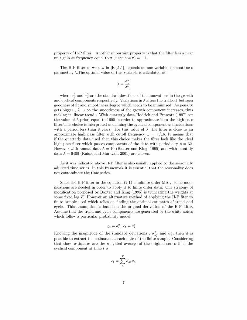
The H-P �lter as we saw in [Eq.1:1] depends on one variable : smoothnessparameter, �:The optimal value of this variable is calculated as:

� =�2g�2c

where �2g and �2c are the standard devations of the innovations in the growth

and cyclical components respectively. Variations in � alters the tradeo¤ betweengoodness of �t and smoothness degree which needs to be minimized. As penaltygets bigger , � ! 1 the smoothness of the growth component increases, thusmaking it linear trend . With quarterly data Hodrick and Prescott (1997) setthe value of � priori equal to 1600 in order to approximate it to the high pass�lter:This choice is interpreted as de�ning the cyclical component as �uctuationswith a period less than 8 years. For this value of � the �lter is close to anapproximate high pass �lter with cuto¤ frequency ! = �=16: It means thatif the quarterly data used then this choice makes the �lter look like the idealhigh pass �lter which passes components of the data with periodicity p = 32.However with annual data � = 10 (Baxter and King, 1995) and with monthlydata � = 6400 (Kaiser and Maravall, 2001) are chosen.

As it was indicated above H-P �lter is also usually applied to the seasonallyadjusted time series. In this framework it is essential that the seasonality doesnot contaminate the time series.

Since the H-P �lter in the equation (2.1) is in�nite order MA , some mod-i�cations are needed in order to apply it to �nite order data. One strategy ofmodi�cation proposed by Baxter and King (1995) is truncating the weights atsome �xed lag K: However an alternative method of applying the H-P �ter to�nite sample used which relies on �nding the optimal estimates of trend andcycle. This assumption is based on the original derivation of the H-P �lter.Assume that the trend and cycle components are generated by the white noiseswhich follow a particular probability model,

gt = agt ; ct = act

Knowing the magnitude of the standard deviations , �2agtand �2act then it is

possible to extract the estimates at each date of the �nite sample. Consideringthat these estimates are the weighted average of the original series then thecyclical component at time t is:

ct =TXh

dhtyh

7

where h is lead/lag index. The weights of the �lter sum to zero,TXh

dht = 0.

The modi�ed �lter behaves as the ideal �lter towards to the middle of the series.But near the end points the gain functions di¤er sharply from each other. Thisproblem is going to be mentioned below.

2.2 Baxter-King Filter

While high pass �lter removes low frequencies from the data , band pass �lterremoves both low an high frequencies from the time series. Based on the Burnsand Mitchell�s (1946) de�nition of the business cycle Baxter and King (1995) de-velop method for measuring the business cycle which isolates the business cyclecomponents bu applying the moving average to the macroeconomic data. Theband pass �lter designed by Baxter and King (1995) (B-K) passes through thecomponents of time series with �uctuations between 6 (18 month) and 32 (96month) quarters, removing higher and lower frequencies. They require 6 obec-tives which the �lter should meet: 1) the �ter should extract a speci�ed rangeof periodicities; 2) ideal band pass �lter should not introduce phase shift; 3)�lter should be optimal approxiamtion to the band pass�lter; 4) approximationof the �lter should result in a stationary time series thus to be able to eliminatethe quadratic trend from the series; 5) the method should yield businss cyclecomponent that are unrelated to the length of the sample period; 6) the methodshould be operational.

The method proposed by Baxter and King (1995) relies on the use of thesymmetric �nite odd-order M = 2K + 1 moving average such that:

y�t =KX

h=�Kahyt�h =

= a0yt +

KXh=1

ah (yt�h + yt+h) (2.2)

which takes the form of a 24- quarter MA when applied to the quarterlydata.

y�t =

12Xh=�12

ahyt�h = a(L)yt

The set of M weights ah is obtained by truncating the ideal �lter weights atM under the frequency response function constraint:

H0 = �t

(N�1)=2Xh=�N=2

ah

8

where N is the number of data points and �t is the sampling periodicity.The frequency response function is built such that at ! = 0 H(0) = 0 for bandpass and high pass �lters and H(0) = 1 for low pass �lters.

The B-K �lter coe¢ cients are driven from the following maximization prob-lem (Noullez and Iacobucci, 2005):

min

(2�t)�1Z�(2�t)�1

�����

KXh=�K

aB�Kh � aidealh

!e�i2�n!�t2

�����2

d!

Solving the maximization problem subject to the (2.2) shows that B-K co-e¢ cients are equal to the ideal �lter coe¢ cients shifted by some constant:

aB�Kh = aidealh +H(0)��t

PKh=�K a

idealh

M�t

Since the �lter depends on M and not on N the performance of the �lterdoes not change as the number of the observations increase.

The B-K �ter has some desirable properties. Because of the symmetrycityproperty the �lter does not present phase shift. Next being of constant �nitelength the �lter is stationary. Another desirable property of the �lter we can seefrom the following implications made by Baxter and King (1995). Consideringthe lag operator a(L) =

PKh=�K ahL

h and applying furher simpli�cations theyshow that their �lter can be factorized as:

a(L) = �(1� L)(1� L�1) K(L)

where K(L) is symmetric moving average with K � 1 lags and leads. Tusthe �lter is able to render stationarity to the time series which contain up totwo unit roots. Further the �lter is incencitive to deterministic trends, so thatit is not used in the edges of the series.

Additionally, adding the �lter to the time series results in the lost of Kobservations both in the beginning and in the end of the series. But choosinglow values for K results in poor approximation of the �ter to the ideal high pass�lter. Thus in order to apply the truncation to the �lter lag , K choice shoulddepend on the length of the data and necessity of how well the �lter should beapproximated. The authors propose putting K � 12; without considering thenumber of observations, sampling frequencs or the band to be extracted, sincea value of K = 12 for the passband (6, 32) quarters is found to be basicallyequivalent to higher values as 16 or 20. Equatng K=12 would thus mean loosing24 observaions from the series

9

3 Problems Associated with Hodrick- PrescottFilter

Above some characteristics of H-P �lter were revised. However there are somedrawbacks associated with H-P �lter. The main problems with H-P which werehighlighted by researchers are the poor approximation of the �lter near theendpoints and the spurious e¤ect it can produce when applied to the series. Inthis part we are going to see these problems in more details.Another problems associated with the �lter is the presence of leakage and

compression when applied to the time series. As it was indicated above forquarterly data setting � = 1600 the �lter can well approximate the ideal high-pass �lter with cut-o¤ frequency ! = �=16. Applying both the ideal highpass and H-P �lter to the data one can observe a rounded peak in the H-P�lter.(Pedersen, 2001 ) which is due to the leakage and the compression of theH-P �lter. Leakage refers to the phenomenon that the �lter passes throughthe frequencies which it was designed to supress whereas compression is thetendency that the �lter has less than unit frequency response for frequenciesabove the cut-of frequency, !.

3.1 End Point Estimation

As it was already mentioned one of the signi�cant critics of the H-P �lter isrelated to its poor approximation near the end points. Above the application ofthe H-P �lter to the �nite samples by Baxter and King was already reviewed.It is shown that in the beginning of the sample period the �lter dht has quitedi¤erent properties that the ideal high pass �lter. Also phase shift is observedin the beginning of the sample. But towards the middle of the series the H-P�lter behaves very close to the ideal band-pass �lter.

In order to evaluate the e¤ect of the �lter they choose AR(1) process:

yt = �yt�1 + at

where the variance of the innovations is V ar(at) = 1 and � = 0:95: Afterapplying the �lter to the series the variance of the observaations di¤er thoughin the real data this pattern is not observed. Their investigation shows thatH-P �lter does not generate as many useful estimates of the cyclical componentas there are data points. That is the �lter weights start to settle down after 12observations.

Another analysis of the revision implied by H-P �ltering was carried outby Kaiser and Maravall (1999). Two features of the revision analyzed are: 1)magnitude and 2) duration of the revision, i.e. the value of K at which the �ltercan be safely truncated. In order to carry the analysis WK version of the �lteris used.Also it should be indicated that the analysis are carried by applying the

10

H-P �lter to the X11-SA series. Assuming that the process is following theARIMA process

�(B)rdyt = �(B)at

with 0 < d < 4, �(B) stationary and �(B) invertible.

After the simpi�cations the estimator of the estimator of the cycle becomes:

bct = �(B;F )at =

�kc(HP )

r4�(B)�H�P (B)�(B)�H�P (B)

�at+2

where kc = V ar(ct)=V ar(at). Analysis of the equation show that the spec-trum of the estimator is determined partially by the structure of the H-P �lterand and partially by the dynamic structure of the series. Thus using the spectralexpression of the estimator the revision of the estimator is found to be:

rtjt =

KXh=�K

�hat+h

Setting the variance of the innovations equal to 1 the variance of the revisionis

V ar(rtjt ) =

KXh=�K

(�h)2

Applying the analysis to three models, white noise, random walk, and IMA(2,2), the magnitude of the revision and duration of the revision, that is the num-ber of the periods needed for the estumatior to converge are exhibited. It wasfound out that the magnitude of the revision was approximately 34% of theone period-ahead foerecast , implying that magnitude was not negligible. As tothe revision period, for all three methods it lasted more than to years (Reginaand Maravall, 2001). Since the H-P �lter is often applied to the seasonally ad-justed X11 series as it was aplready noted above, where �lter X11 also producesrevisions the revisions associated with the analysis would re�ect the combinede¤ect of the two �ltter. In order to see this e¤ect the authors consider the whitenoise case. That is, since yt = at the revision analysis would illustrate �pure�lter� e¤ect. This shows that after 13 quarters 95% of the revision variancedisappers. Thus it takes 13 observations for the �lter to settle down. Also �nalanalysis show that highly moving trends and seasonals are subject to bigger,longer-lasting revisions.

As we can see from the analysis it takes the �lter 12 or 13 observationsto settle down. Thus it iwould be straightforward to drop these amount ofobservations both in the beginning and in the end of the series. But in thiscase H-P �lter is not preferred to B-K �lter since the same or more numberobservations are lost by applying both �lters to the series.

11

3.2 Spurious E¤ect

Another most critisized feature of the H-P �lter is the spurious e¤ect it canproduce when applied to the series.Less smooth comparing with B-K �lter. By construction the spectrum of the

H-P �lter is zero at zero frequency, as well as at seasonal frequencies, ! = �=2and ! = �. This �xed structure results in spurious e¤ect (Kaiser and Maravall,2001). That is two peak structure of the spectrum results in the possibbility ofobtaining spurious autocorrelation structure of the series.. Also the presence ofthree zeros will induce peaks in the spectrum which would result in a spuriousperiodic cycle

In order to detect the spurious crosscorrelation in the H-P �ltered seriesKaiser and Maravall (1999) carry simulations for white noise and random walkseries. For the �rst series no spurious crosscorrelation was detected , althoughfor random walk a moderate spurious e¤ect was detected. The spurious autocor-relations were analyzed using calibration technique, i.e. validating the econmicmodel by comparing the previous ACF with the one implied by the observedeconomic variable. To carry the analysis the following AR(2) process was con-sidered:

(1� 1:293B + :49B2)ct = at

Detrending the SA series with H-P �lter the ACF for observed series wasobtained. The anlysis showed that the ACF of the cycle contained in the se-ries was considerably di¤erent that the one obtained by �ltering, thus showingsigni�cant distortions implied by the H-P �ltering.

For the anaysis of the spurious periodic cycles the series spectrum was con-sidered, in order to see which variation was actually passed. For this purposewhite noise and random walk series were used. For the white noise input itwas found that the peaks of the AR process which was �t to the �ltered seriescapture the peaks of the spectrum of the �ltered white noise series. It was con-cluded that H-P �lter is likely to produce spurious periodic cycles when appliedto white noise series.

In Figures 8, 9, 10 we can see the H-P �ltered series compared with B-K�ltered series. Though there is a close correspondence between the �ltered series,the B-K �ltered series looks more smooth. As well as in the B-K�ltered serieswe can not observe the two-peakedness as we do in H-P �ltered series. Thusthe presence of the spurious results are less probable in the series by applicationB-K �lter to the time series.

4 Summary

The purpose of this paper was to see the review the critics of the Hodrick-Prescott �lter introduced in the literature and compare it to the �lter propsed

12

by Baxter and King (1995). Despite the fact that the �lter has several desir-able features which we saw above there are some problems associated with theapplication of H-P �lter to the time series which limits the usefullness of the�lter for the analysis of the data. These problems included mainly the end pointestimation and spurious e¤ect. That is in the beginning and towards to the endof the data the behavior of the �lter is not reliable, thus some points from thedata are to be dropped o¤. Anther problem associated with the �lter is thespurious e¤ect it could produce when applied to the series.

Another �lter which was represented by Baxter and King (1995) was re-viewed as well. Form the discussion above it could is concluded that thoughB-K �lter also contain the problem of lost of the data in the beginning and in theend of the series. But since the �lter does not produce as much spurious e¤ectas H-P �lter does using B-K �lter in business cycles would be more appropriate.

13

Literature

1. A. Guay and P. St-Amant. Do the Hodrick-Prescott and Baxter-KingFilters Provide a Good Approximation of Business Cycles? CREFE,Université du Québec à Montréal, Cahiers de recherche CREFE / CREFEWorking Paper No. 53, 1997

2. A. Noullez and A. Iacobucci. A frequency-selective �lter for short-lengthtime series. Computing in Economics and Finance 2004 128, Society forComputational Economics, 2005.

3. F. Canova. Detrending and Business Cycle Facts. Journal of MonetaryEconomics, Vol. 41, pg 475-512, 1998.

4. M. Baxter and R.G. King. Measuring business cycles: Approximate band-pass �lters. The Review of Economics and Statistics, 81(4):575�93, 1999.

5. R.J. Hodrick and E.C. Prescot. Postwar US business cycles: an empiricalinvestigation. Journal of Money, Credit, and Banking, 29(1):1�16, 1997.

6. R. Kaiser and A. Maravall. Estimation of the Business Cycle: A Modi�edHodrick-Prescott Filter. Banco de España- Servicio de Estudios, Docu-mento de Trabajo no 9912,1999.

7. R. Kaiser and A. Maravall. Measuring Business Cycles in Economic TimeSeries (Lecture Notes in Statistics, Vol. 154), Springer-Verlag, New York,2001.

8. T. Cogley and J. Nason. E¤ects of the Hodrick-Prescott Filter on Trendand Di¤erence Stationary Time Series: Implications for Business CycleResearch. Journal of Economic Dynamics and Control, Vol. 19, pages253-278, 1995.

9. T. Pedersen. The Hodrick-Prescott Filter, the Slutzky E¤ect, and the Dis-tortionary E¤ect of Filters. Journal of Economic Dynamics and Control,Vol. 25, pages 1081-1101, 2001.

14

5 Appendix

5.1 Matlab Routines

5.1.1 Baxter King Filter

%Program name: BPFfunction yf=bpf(y,up,dn,K);%bpf.m%Program to compute bp filter%Inputs are:%y: data(rows=observations,columns=series)%up:period corresponding to highest frequency (e.g.,6)%dn: period corresponding to lowest frequency (e.g.,32)%K: number of terms in approximating moving average%[calls filtk.m (filter with symmetric weights) as subroutine],

The%frequencies are chosen according to Burns and Mitchell. With quarterly%data x=[32 6]. Since I am using monthly data x vector is [96 18].up=96; %dn=18;K=12;x=[up dn];disp(�)disp(�bpf(y,up,dn,K):band pass filtering of series y with symmetric

MA(2K+1)�)disp(�)disp(� for additional information see:�)disp(�)disp(� M.Baxter and R.G. King�)disp(�)disp(� Measuring Business Cycles:�)disp(� Approximate Band-Bass Filters�)disp(� for Macroeconomic Time Series�)disp(�)disp(�Filter extracts components between period of:�)disp(� up dn�)disp(x)%pause(2)if(up>dn)disp(�Periods reversed: switcing indices up & dn�)disp(�)dn=x(1);up=x(2);endif (up<2)

15

up=2;disp(�Higher periodicity >max: Setting up=2�)disp(�)end%convert to column vector[r c]=size(y);if(r<c)y=y�disp(�There are more columns than rows: Transposing data matrix�)disp(�)end%Implied Frequenciesomubar=2*pi/up;omlbar=2*pi/dn;% An approximate low pass filter , with a cutoff frequency of �ombar�,%has a frequency response function%alpha(om)=a0+2*a1cos(om)+...+2*aKcos(K om)%and the ak�s are given by:%a0=ombar/(pi) ak=sin(k ombar)/(k pi)%where ombar is the cutoff frequency.% A band pass filter is the difference between two%low pass filter,bp(L)=bu(L)-bl(L) with bu(L) being filter with

high cutoff%point and bl(L) being filter with low cutoff%point. Thus the weights are differences of weights for two low

pass%filters.% Construct filter weights for bandpass filter (a(0)...a(K)).akvec=zeros(1,1:K+1);akvec(1)=(omubar-omlbar)/(pi); %weight at k=0for k=1:K;akvec(k+1)=(sin(k*omubar)-sin(k*omlbar))/(k*pi); %weight at k=1,2,...Kend%Impose constraint on frequency response at om=0%If high pass filter this amounts to requiring that weights sum

to zero%If low pass filter this amounts to requiring that weights sum to

oneif (dn>1000)disp(�dn>1000:assuming low pass filter�)phi=1;elsephi=0;end%Sum of weights without constrainttheta=akvec(1)+2*sum(akvec(2:K+1));

16

%amount to add to each nonzero lag/lead to get sum=phitheta=phi-(theta/(2*K+1));%adjustment of weightsakvec=akvec+theta;%filter the time seriesyf=filtk(y,akvec);if(r<c)yf=yf;end

%Program name : FILTK.Mfunction yf=filtk(y,a);%Filter data with a filter with symmetric filter with weights data

is%organized (rows=obs,columns=series)%a=[a0,a1,...,aK];K=max(size(a))-1; %max lag;T=max(size(y)); %number of observations;%Set vector of weightsavec=zeros(1,2*K+1);avec(K+1)=a(1);for i=1:K;avec(K+1-i)=a(i+1);avec(K+1+i)=a(i+1);endyf=zeros(y);for t=K+1:1:T-Kyf(t,:)=avec*y(t-K:t+K,:);end

5.1.2 Hodrick- Prescott Filter

%Program Name: HPF% If x is a column vector of length LENGTH% xtr=HP_matnx; delivers the HP-trend and% xhp=x-xtr; delivers the HP-filtered series% This program computes HP_mat, given the length of% some given column vector x% I will use HP_LAMBDA = 6400, unless you assign a different value

beforehand.HP_LAMBDA = 6400;disp(�If x is a column vector of length LENGTH,�);disp(�xtr=HP_matnx; delivers the HP-trend and�);disp(�xhp=x-xtr; delivers the HP-filtered series�);disp(�This program computes HP_mat, given the length of�);

17

disp(�some given column vector x�);LENGTH = max(size(x));if ~exist(�HP_LAMBDA�),HP_LAMBDA = 1600;end;% The following piece is due to Gerard A. PfannHP_mat = [1+HP_LAMBDA, -2*HP_LAMBDA, HP_LAMBDA, zeros(1,LENGTH-3);-2*HP_LAMBDA,1+5*HP_LAMBDA,-4*HP_LAMBDA,HP_LAMBDA, zeros(1,LENGTH-4);zeros(LENGTH-4,LENGTH);zeros(1,LENGTH-4),HP_LAMBDA,-4*HP_LAMBDA,1+5*HP_LAMBDA,-2*HP_LAMBDA;

zeros(1,LENGTH-3), HP_LAMBDA, -2*HP_LAMBDA, 1+HP_LAMBDA ];for iiiii=3:LENGTH-2;HP_mat(iiiii,iiiii-2)=HP_LAMBDA;HP_mat(iiiii,iiiii-1)=-4*HP_LAMBDA;HP_mat(iiiii,iiiii)=1+6*HP_LAMBDA;HP_mat(iiiii,iiiii+1)=-4*HP_LAMBDA;HP_mat(iiiii,iiiii+2)=HP_LAMBDA;end;xtr=HP_matnx;xhp=x-xtr;

18

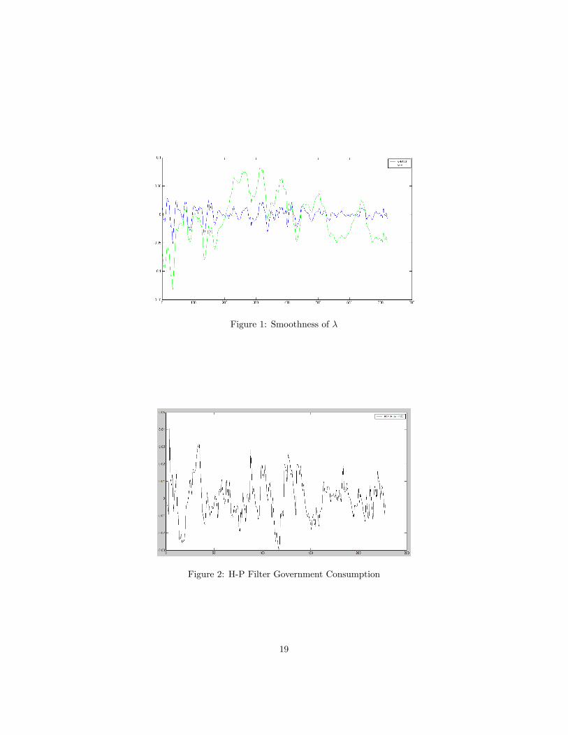
Figure 1: Smoothness of �

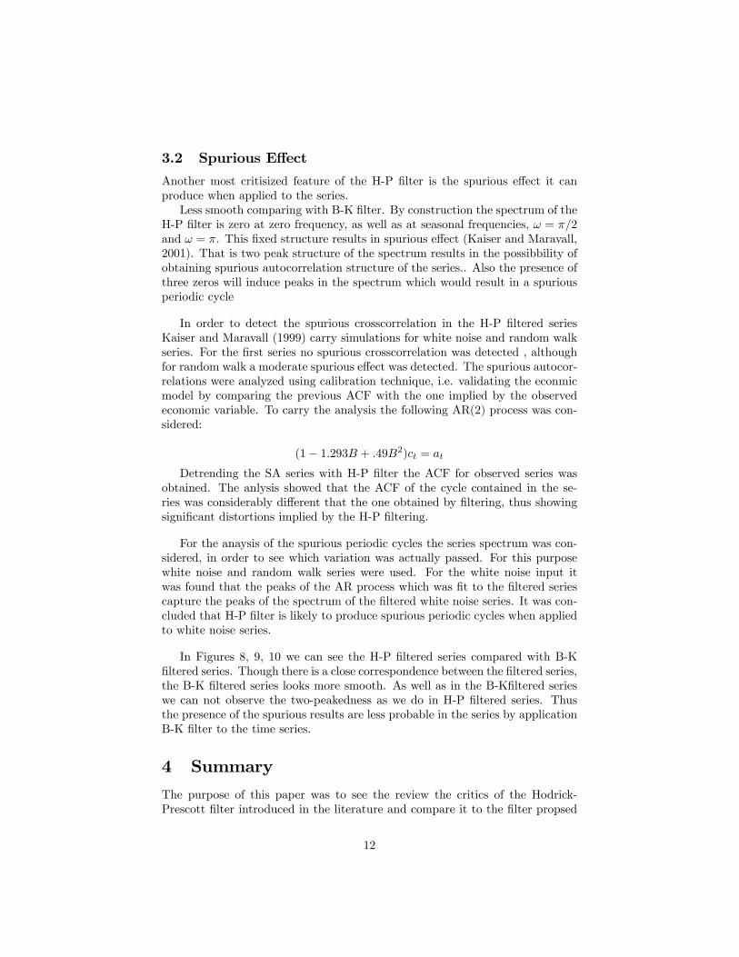
Figure 2: H-P Filter Government Consumption

19

Figure 3: H-P Filter, Gross National Product

Figure 4: H-P Filter, Government Investment

20

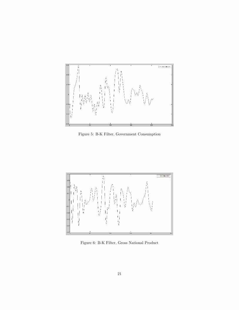
Figure 5: B-K Filter, Government Consumption

Figure 6: B-K Filter, Gross National Product

21

Figure 7: B-K Filter, Government Investment

Figure 8: H-P Filter vs B-K Filter

22

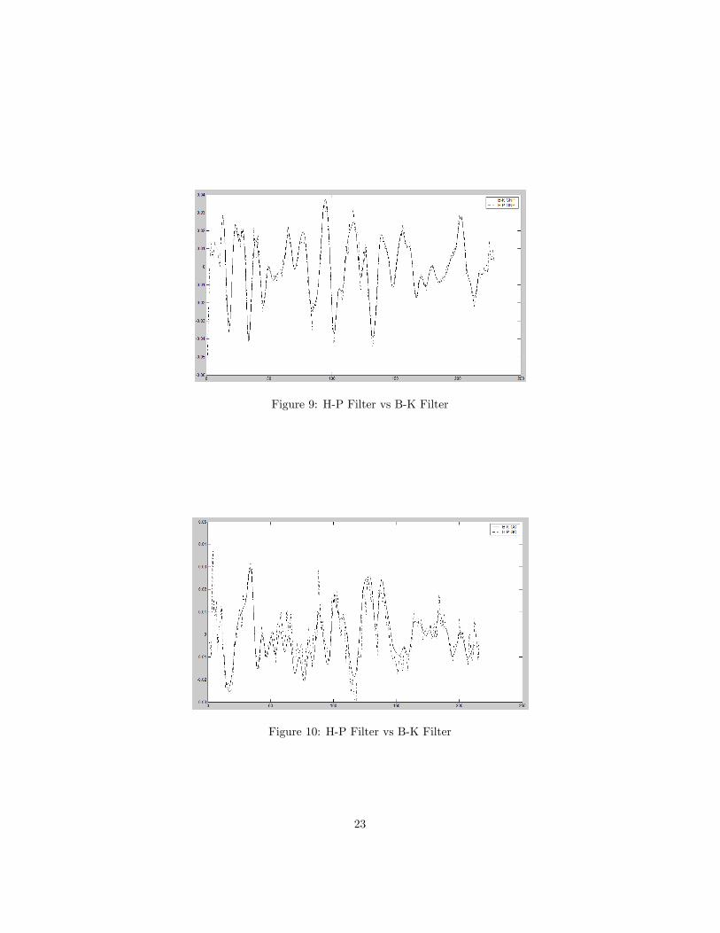
Figure 9: H-P Filter vs B-K Filter

Figure 10: H-P Filter vs B-K Filter

23