Robotics

Notes

Holger Findling

My CI Group

Robotics

© 2015. My CI Group. All rights reserved.

Contents Introduction ................................................................................................................................................... 6

Fundamentals ................................................................................................................................................ 7

Basic Analog Circuits ............................................................................................................................... 7

Voltage Divider ..................................................................................................................................... 9

Angular Position of a Potentiometer ................................................................................................... 11

Powering an LED ................................................................................................................................ 12

Analog and Digital Signals ..................................................................................................................... 13

Basic Mechanics ..................................................................................................................................... 14

Velocity ............................................................................................................................................... 14

Acceleration ........................................................................................................................................ 14

Torque ................................................................................................................................................. 15

Electro-Mechanics .................................................................................................................................. 15

Laplace Transforms ................................................................................................................................ 19

Feedback Circuits ................................................................................................................................ 19

Common Amplifier Configurations .................................................................................................... 20

Servo Systems ............................................................................................................................................. 24

Basic Servo System ................................................................................................................................. 24

Robotic Arm – Gripper with 5 Degree Freedom .................................................................................... 26

Robotic Arm – 6 Degree Freedom .......................................................................................................... 28

Rotation Kinematics .................................................................................................................................... 30

Kinematics .................................................................................................................................................. 31

Rotation about Z axis .......................................................................................................................... 34

Forward Kinematics .................................................................................................................................... 35

Inverse Kinematics ...................................................................................................................................... 36

Software and Sketches ................................................................................................................................ 37

Structure .............................................................................................................................................. 38

setup() ................................................................................................................................................. 38

Control Structures ............................................................................................................................... 38

Further Syntax ..................................................................................................................................... 38

Arithmetic Operators .......................................................................................................................... 38

Comparison Operators ........................................................................................................................ 39

Boolean Operators .............................................................................................................................. 39

Pointer Access Operators .................................................................................................................... 39

Bitwise Operators ................................................................................................................................ 39

Compound Operators .......................................................................................................................... 39

Variables ................................................................................................................................................. 40

Constants ............................................................................................................................................. 40

Data Types .......................................................................................................................................... 40

Conversion .......................................................................................................................................... 41

Variable Scope & Qualifiers ............................................................................................................... 41

Utilities ................................................................................................................................................ 41

Functions ................................................................................................................................................. 41

Digital I/O ........................................................................................................................................... 41

Analog I/O .......................................................................................................................................... 42

Due & Zero only ................................................................................................................................. 42

Advanced I/O ...................................................................................................................................... 42

Time .................................................................................................................................................... 42

Math .................................................................................................................................................... 43

Trigonometry ...................................................................................................................................... 43

Random Numbers ............................................................................................................................... 43

Bits and Bytes ..................................................................................................................................... 43

External Interrupts .............................................................................................................................. 43

Interrupts ............................................................................................................................................. 44

Communication ................................................................................................................................... 44

USB (32u4 based boards and Due/Zero only) .................................................................................... 44

Figure 1- Basic Analog Circuit ..................................................................................................................... 7 Figure 2 - Voltage Divider ............................................................................................................................ 9 Figure 3 – Potentiometer ............................................................................................................................. 10 Figure 4 - LED Circuit ................................................................................................................................ 12 Figure 5 - Signals ........................................................................................................................................ 13 Figure 6 - PWM .......................................................................................................................................... 13 Figure 7 - Servo Motor, RG-SRV 180 ........................................................................................................ 16 Figure 8 – Servo Motor, FS90MG .............................................................................................................. 17 Figure 9 - Amplifier with negative feedback .............................................................................................. 19 Figure 10 - Amplifier with positive feedback ............................................................................................. 20 Figure 11 - Chaining Amplifier Circuits ..................................................................................................... 20 Figure 12 - Summing outputs of two amplifiers ......................................................................................... 21 Figure 13 - Equivalent Circuits .................................................................................................................. 22 Figure 14 - Basic Servo System .................................................................................................................. 24

Figure 15 - Robotic Arm, 5 DOF ................................................................................................................ 26 Figure 16 - Robotic Arm, 5 DOF ................................................................................................................ 27 Figure 17 - 4R Geometry ............................................................................................................................ 27 Figure 18 - Robotic Arm 6 DOF and Laser Endpoint ................................................................................. 28 Figure 19 - Robotic Arm, 6 DOF ................................................................................................................ 28 Figure 20 - Robotic Laser Arm Dimensions ............................................................................................... 29

Table 1 - Power ............................................................................................................................................. 8 Table 2 - Angular Position versus Output Voltage ..................................................................................... 11 Table 3 - Specifications, RG-SRV 180 ....................................................................................................... 16 Table 4 - Specifications, FS90MG .............................................................................................................. 18

Introduction

Fundamentals

Control system components are typically comprised of electrical, mechanical, and electromechanical

devices. Together they build our basic servo system and robotics.

Basic Analog Circuits

Figure 1 shows a basic analog circuit comprised of a battery and a resistor. When the resistor is connected

to the battery a closed circuit is created and current (I) flows through resistor (R). By convention we trace

current flow from the positive terminal of the battery to the negative terminal. The negative terminal is

considered a reference point (ground) for the circuit. All voltages are measured in respect to ground.

Figure 1- Basic Analog Circuit

The voltage measured across the resistor is notated as VR (t) and it has the same voltage potential as the

battery voltage; V = 10 volts. We state that the positive terminal of the battery and the resistor are connected

to the same node. The current and voltage relationship can be expressed in regards to time.

VR (t) = I (t) * R

IR (t) / VR (t) = 1 / R

Since the battery voltage is a constant over some period of time, the current is constant over time as well.

Therefore, the time component is often ignored.

VR = I * R

I / VR = I / R

Since resistance is an opposition to current flow the resistor consumes energy. The energy is converted to

heat energy and designers have to ensure that the power ratings of the resistor are observed. Power

consumption is measured in watts.

P = I * VR (watts)

A good design implements a power safety factor of 3:1, however a 2:1 ratio may be sufficient for circuits

using small amount of voltages and currents. Typically resistors are commercially available in 1/8, 1/4, 1/2,

and 1 watt sizes.

Table 1 shows the relationship between resistance and current using a constant 10 volt source. The data

shows that the power consumption decreases as a function of I2 as the resistance increases.

Substitute VR = I * R into

P = I * V

V = I * (I * R)

P = I2 * R

Table 1 - Power

R (ohm) I (amp) P

(Watts)

100 0.100 1.000

200 0.050 0.500

300 0.033 0.333

400 0.025 0.250

500 0.020 0.200

600 0.017 0.167

700 0.014 0.143

800 0.013 0.125

900 0.011 0.111

1000 0.010 0.100

Example:

Given the data in Figure 1

VR = I * R

I = VR / R

I = 10 v / 1000 ohm

I = 0.01 amp or 10 ma

The power consumed PR by resistor R is a measure of current IR and voltage VR.

PR = IR * VR

PR = 0.01 amp * 10 v

PR = = 0.1 watt or 100 mw

The resistor should have a power rating of 1/4 watt using a power safety factor 2:1.

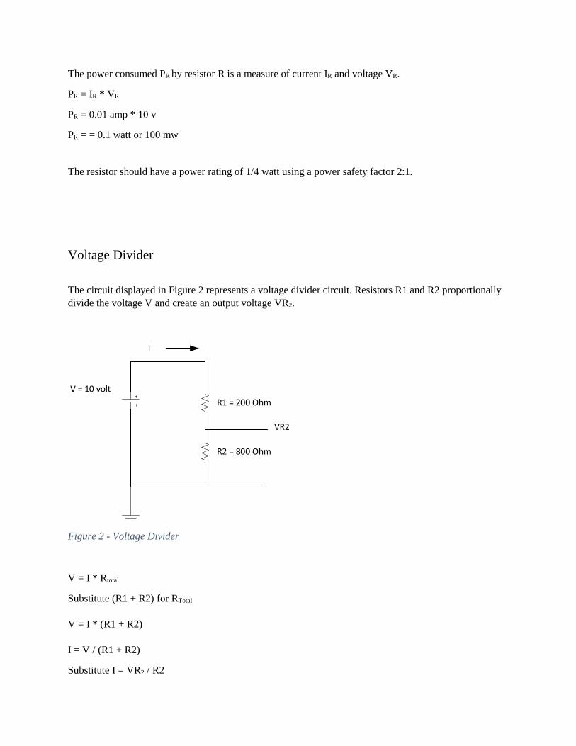
Voltage Divider

The circuit displayed in Figure 2 represents a voltage divider circuit. Resistors R1 and R2 proportionally

divide the voltage V and create an output voltage VR2.

V = 10 volt

R1 = 200 Ohm

I

R2 = 800 Ohm

VR2

Figure 2 - Voltage Divider

V = I * Rtotal

Substitute (R1 + R2) for RTotal

V = I * (R1 + R2)

I = V / (R1 + R2)

Substitute I = VR2 / R2

VR2 / R2 = V / (R1 + R2)

VR2 = V * (R2 / (R1 + R2))

Where

R2 / (R1 + R2) is the voltage divider ratio

Example:

Refer to Figure 2.

V = 10 volts

R1 = 200 ohm, R2 = 800 ohm

VR2 = V * (R2 / (R1 + R2))

VR2 = 10 v * (800 / (200 + 800))

VR2 = 8 volt

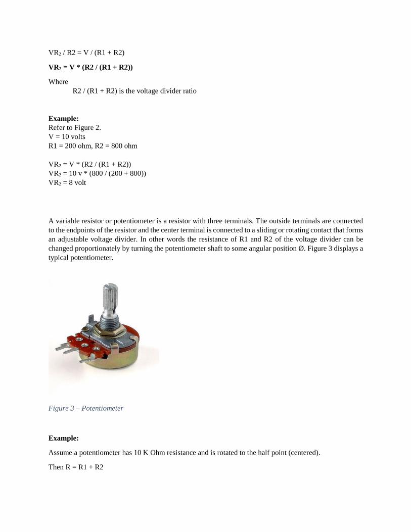
A variable resistor or potentiometer is a resistor with three terminals. The outside terminals are connected

to the endpoints of the resistor and the center terminal is connected to a sliding or rotating contact that forms

an adjustable voltage divider. In other words the resistance of R1 and R2 of the voltage divider can be

changed proportionately by turning the potentiometer shaft to some angular position Ø. Figure 3 displays a

typical potentiometer.

Figure 3 – Potentiometer

Example:

Assume a potentiometer has 10 K Ohm resistance and is rotated to the half point (centered).

Then R = R1 + R2

Where R1 = R2 or 10,000 ohm / 2 = 5000 ohm

If V = 10 volts then

VR2 = V * (R2 / (R1 + R2))

VR2 = 10 * (5000 / (5000 + 5000))

VR2 = 5 volts

Angular Position of a Potentiometer

The voltage divider ratio R2/ (R1 + R2) can be expressed as the angular rotation Ø.

Suppose a 10,000 ohm potentiometer can rotate from 0 to 180 degrees, and the circuit uses a 10 volt

power supply. Table 2 shows the relationship between the angular position and the output voltage.

Table 2 - Angular Position versus Output Voltage

Degrees Radians Resistance Voltage

0 0.0000 0 10.00

45 0.7853 2500 7.50

90 1.5707 5000 5.00

135 2.3560 7500 2.50

180 3.1415 10000 0.00

VR = Kp r

Where Kp is the constant of proportionality between the shaft position and the potentiometer voltage. Kp

equates to the total voltage applied to the potentiometer divided by the maximum angle of rotation Ø max.

Kp = V / Ø max --- V/rad

Example:

Let V = 10 volts and Ø max = 180 deg.

Then

Kp = V / Ø max

Kp = 10 v / 180 degrees

Kp = 10 v / 3.14 Rad

Kp = 3.1847 (V/ Rad)

Example:

Suppose the potentiometer is turned 90 degrees or PI/2 Radians.

Then VR = KP r

VR = (3.1847 V/ Rad)* (PI / 2 Rad)

VR = 4.999979 volts or ~ 5.0 volts

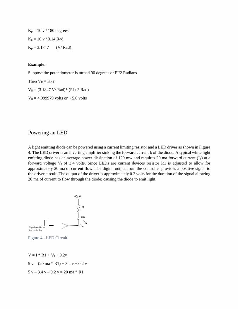
Powering an LED

A light emitting diode can be powered using a current limiting resistor and a LED driver as shown in Figure

4. The LED driver is an inverting amplifier sinking the forward current If of the diode. A typical white light

emitting diode has an average power dissipation of 120 mw and requires 20 ma forward current (IF) at a

forward voltage Vf of 3.4 volts. Since LEDs are current devices resistor R1 is adjusted to allow for

approximately 20 ma of current flow. The digital output from the controller provides a positive signal to

the driver circuit. The output of the driver is approximately 0.2 volts for the duration of the signal allowing

20 ma of current to flow through the diode; causing the diode to emit light.

+5 v

Signal send from the controller

LED

R1

Figure 4 - LED Circuit

V = I * R1 + Vf + 0.2v

5 v = (20 ma * R1) + 3.4 v + 0.2 v

5 v – 3.4 v – 0.2 v = 20 ma * R1

R1 = 1.4 v / 0.02 amp

R1 = 70 ohms

Analog and Digital Signals

Figure 5 displays a digital signal comprised of a stream of continuous pulses equally spaced apart. The

frequency of the signal is determined by

Frequency = 1 / Time

Time = t2 – t1

Amplitute

Gnd

t0 t1 t2

50 % Rise Time

Figure 5 - Signals

The pulse width is typically measured at the 50 percent level of the rise time of the pulse. A signal send to

a servo amplifier is usually pulse width modulated, implying that the pulse width of the signal specifies

the angular position of the servo motor. An advantage of using pulse width modulation is that the angular

position is not functionally dependent on the amplitude of the signal, which may vary considerable from

system to system.

Reference Signal

Pulse Width Modulated

Signal

Figure 6 - PWM

Example:

What is the frequency of a signal where t1 = 10 usec and t2 = 50 usec?

Time = t2 – t1

Time = 50 usec – 10 usec

Time = 40 usec

Frequency = 1/ 40 usec

Frequency = 0.025 MHz or 25 KHz

Example:

Suppose a servo motor can rotate from 0 to 180 degrees, and 1 millisecond represents 0 degrees and 2

milliseconds represents 180 degrees. Determine the angular position given a 1.2 millisecond signal.

(180deg – 0deg) / (180 – X) = (2msec – 1msec) / (2msec - 1.2msec)

180 / (180 – x) = 1 / 0.8

X = 180 – 0.8 * 180

X = 36 degrees

Basic Mechanics

Velocity

The velocity of a rigid object is the rate at which its position changes with time.

V (t) = (r2 – r1) / (t2 – t1) (m/sec)

V = dr / dt

Acceleration

Often the velocity of a moving object changes either in magnitude or direction, or both. The object has

acceleration which is the rate of change of its velocity with time.

a = dv / dt (m/sec2)

Torque

In translational motion we associate a force with the linear acceleration of a body.

ForceMass

Acceleration

F = m * a (N m)

Example:

Determine the acceleration of a 1 Kg mass when a 1 Newton force is applied.

F = m * a

1 N = 1 Kg * a

a = 1N / 1 Kg 1 m/ sec2

In rotational motion we associate torque with the angular acceleration of a body when a force is applied to

a moment arm r.

Ί = r x F (N m)

Electro-Mechanics

Figure 5 and Figure 6 display typical servo motors used for light weight robotic projects and hobby kits.

Their specifications are provided in Table 3 and Table 4. Of particular interest are the Stall Torque and No

Load Speed specifications required to calculate the transfer functions for the basic servo system in section

Servo Systems.

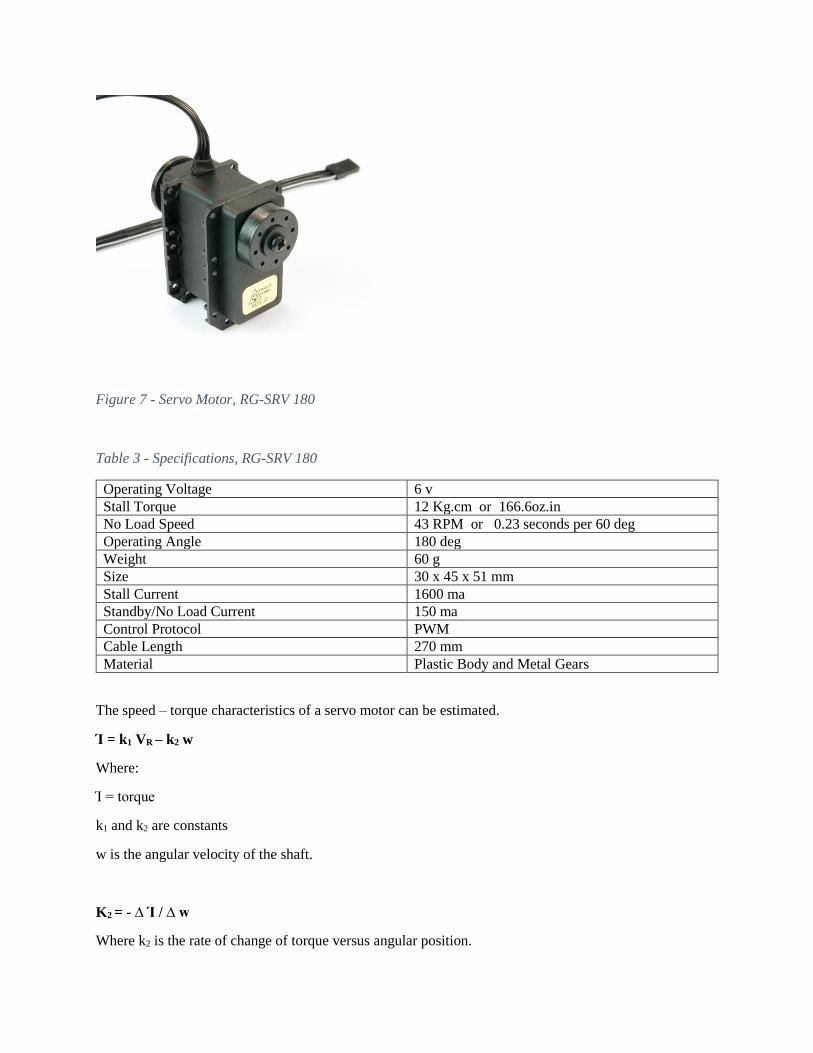
Figure 7 - Servo Motor, RG-SRV 180

Table 3 - Specifications, RG-SRV 180

Operating Voltage 6 v

Stall Torque 12 Kg.cm or 166.6oz.in

No Load Speed 43 RPM or 0.23 seconds per 60 deg

Operating Angle 180 deg

Weight 60 g

Size 30 x 45 x 51 mm

Stall Current 1600 ma

Standby/No Load Current 150 ma

Control Protocol PWM

Cable Length 270 mm

Material Plastic Body and Metal Gears

The speed – torque characteristics of a servo motor can be estimated.

Ί = k1 VR – k2 w

Where:

Ί = torque

k1 and k2 are constants

w is the angular velocity of the shaft.

K2 = - ∆ Ί / ∆ w

Where k2 is the rate of change of torque versus angular position.

Example:

Given the RG SRV 180 servo motor specification determine constant k1 and k2.

K1 = stall torque at rated voltage / max voltage

K1 = 12 Kg cm / 6 v

K1 = 2 Kg cm / v

K2 = stall torque / no-load speed.

K2 = 12 Kg cm / (0.23 sec / 60 deg)

K2 = 0.8695 Kg cm / (sec/deg)

Calculate the maximum torque applied to the shaft with zero load.

Ί = k1 VR – k2 w

Ί = 2 (Kg cm / v) * 6 v – 0.8695 (Kg cm / (sec / deg)) (0.23 sec / 60 deg)

Ί = 12 (Kg cm) – 0.00333 (Kg cm)

Ί = 11.996 (Kg cm) 12 (Kg cm)

Figure 8 – Servo Motor, FS90MG

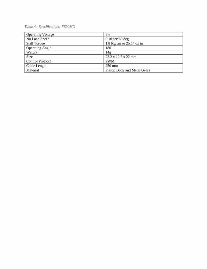
Table 4 - Specifications, FS90MG

Operating Voltage 6 v

No Load Speed 0.10 sec/60 deg

Stall Torque 1.8 Kg cm or 25.04 oz in

Operating Angle 180

Weight 14g

Size 23.2 x 12.5 x 22 mm

Control Protocol PWM

Cable Length 250 mm

Material Plastic Body and Metal Gears

Laplace Transforms

The translation of a system description into the language of mathematics is called modeling. Modeling is a

level of abstraction of the real world whereby the important aspects of a problem are isolated and the minor

ones are ignored. As a result simplicity with sufficient accuracy is obtained. It is important that engineers

understand how far the model deviates from the real world to minimize errors.

By performing a Laplace transform our time-based equations are converted to the s-domain where the

equations become linear algebraic equations. Time and frequency response of a feedback control system

are more readily obtained in the s-domain. Stability of the feedback control system to be modeled requires

that the roots of the characteristic equations reside to the left of the imaginary axis where the components

of the natural system response decay with time. When the roots of the characteristic equations reside on the

right side of the imaginary axis then the system may oscillate and grow in time causing potential damage.

In this case the system is considered unstable and it is not safe for operation.

The Laplace transform of a function is provided below. Refer to a Differential Calculus book for further

information performing various transforms.

𝐿[f (t)] = F(s)

𝐹(𝑠) = ∫ 𝑓 (𝑡) 𝑒−𝑠𝑡∞

0−

𝑑𝑡

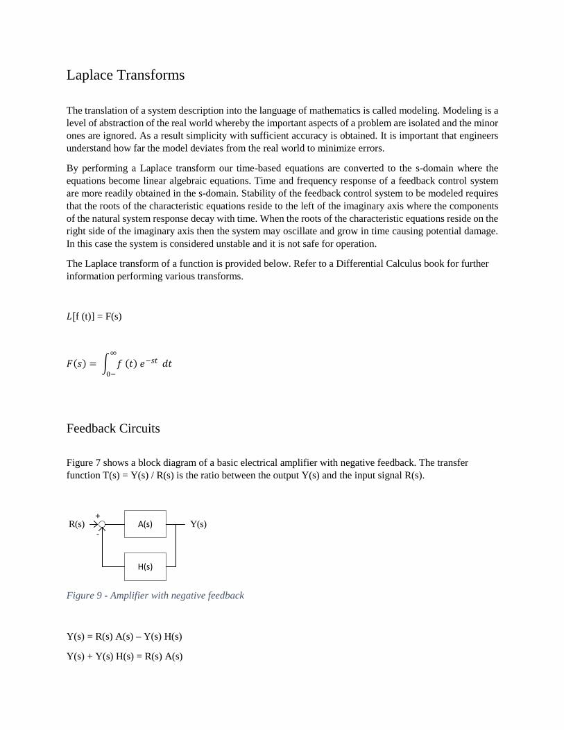
Feedback Circuits

Figure 7 shows a block diagram of a basic electrical amplifier with negative feedback. The transfer

function T(s) = Y(s) / R(s) is the ratio between the output Y(s) and the input signal R(s).

R(s)+

A(s) Y(s)

H(s)

-

Figure 9 - Amplifier with negative feedback

Y(s) = R(s) A(s) – Y(s) H(s)

Y(s) + Y(s) H(s) = R(s) A(s)

Y(s) (1+ H(s)) = R(s) A(s)

Y(s) / R(s) = A(s) / (1+H(s)) where T(s) = Y(s) / R(s)

Figure 8 shows a basic block diagram of an electrical amplifier with positive feedback. Observe that the

negative feedback circuit in Figure 7 results in A(s) / (1+H(s)) and the positive feedback circuit in Figure

8 results in A(s) / (1-H(s)).

R(s)+

A(s) Y(s)

H(s)

+

Figure 10 - Amplifier with positive feedback

Y(s) = R(s) A(s) + Y(s) H(s)

Y(s) - Y(s) H(s) = R(s) A(s)

Y(s) (1 - H(s)) = R(s) A(s)

Y(s) / R(s) = A(s) / (1-H(s)) where T(s) = Y(s) / R(s)

The standard notation for an amplifier with feedback is shown below.

T(s) = A(s) / (1+ H(s))

Common Amplifier Configurations

Figure 9 shows amplifiers chained together. The input signal R(s) is applied to A1(s) and its output is

further amplified by A2(s). Here A1(s) may represent the transfer function for a differential amplifier and

A2(s) may represent the transfer function for a power amplifier driving a servo motor.

R(s) A1(s) Y(s)A2(s)

Figure 11 - Chaining Amplifier Circuits

Y(s) = R(s) A1(s) A2(s)

T(s) = (Y(s) / R(s)) (A1(s) A2(s)

R(s)

A1(s)

Y(s)

A2(s)

+

+

Figure 12 - Summing outputs of two amplifiers

Y(s) = R(s) A1(s) + R(s) A2(s)

T(s) = (Y(s) / R(s)) (A1(s) + A2(s))

Example:

Provide the transfer function for the diagram below.

A(s) = 10 / (s + 10)

R(s) A(s) Y(s)+ + -

-

Y(s) = (A(s) R(s) / (1 + A(s)) – R(s)

T(s) = Y(s) / R(s) = (A(s) / (1 + A(s)) -1

T(s) = (10 / (s + 10)) / (1 + (10 / (s + 10)) - ((s + 10) / (s + 10))

T(s) = -s / (s + 20)

Note:

The diagrams in Figure 11 are equivalent and represent the basic amplifier with negative feedback.

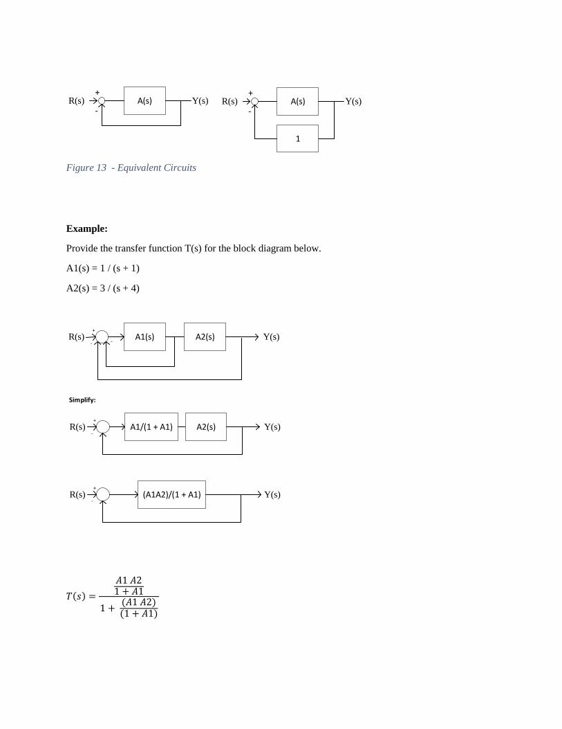
R(s)+

A(s) Y(s)-

R(s)+

A(s) Y(s)-

1

Figure 13 - Equivalent Circuits

Example:

Provide the transfer function T(s) for the block diagram below.

A1(s) = 1 / (s + 1)

A2(s) = 3 / (s + 4)

R(s) A1(s) Y(s)A2(s)--

+

R(s) A1/(1 + A1) Y(s)A2(s)-

+

R(s) (A1A2)/(1 + A1) Y(s)-

+

Simplify:

𝑇(𝑠) =

𝐴1 𝐴21 + 𝐴1

1 + (𝐴1 𝐴2)(1 + 𝐴1)

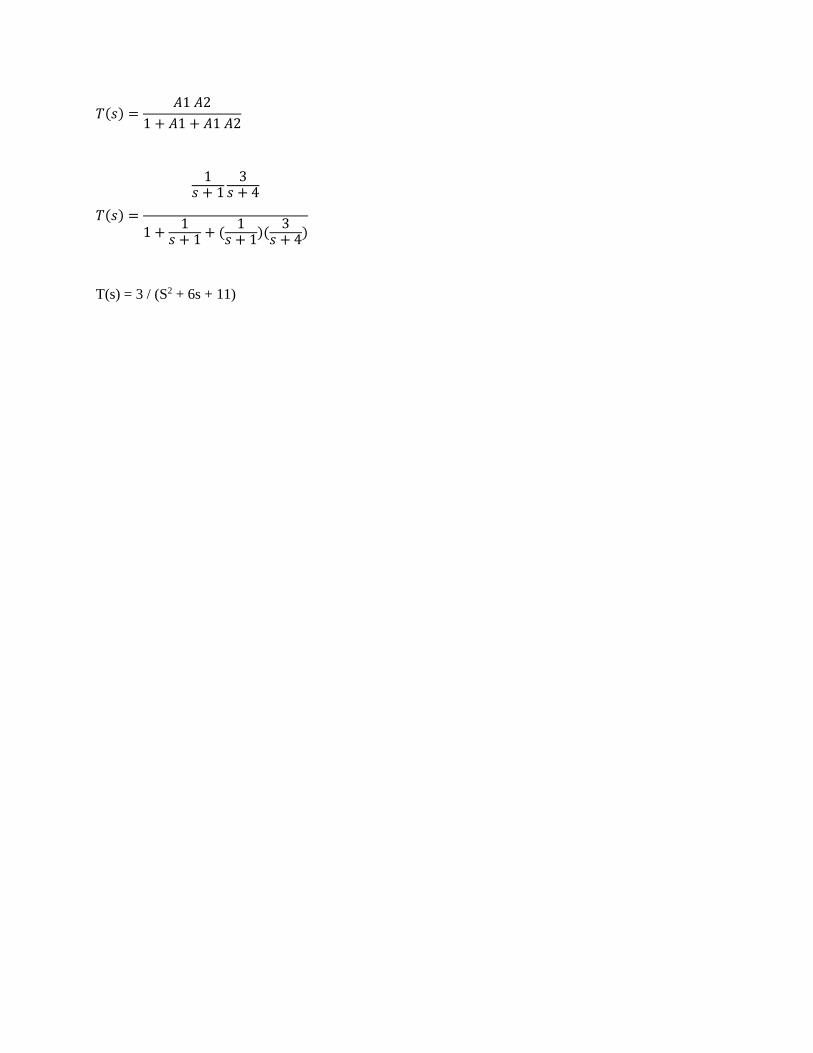
𝑇(𝑠) =𝐴1 𝐴2

1 + 𝐴1 + 𝐴1 𝐴2

𝑇(𝑠) =

1𝑠 + 1

3𝑠 + 4

1 +1

𝑠 + 1 + (1

𝑠 + 1)(3

𝑠 + 4)

T(s) = 3 / (S2 + 6s + 11)

Servo Systems

Basic Servo System

A2A1+-

12 Vdc 12 Vdc

Angular Positioning

Angular Positioning Feedback

Servo Motor

Load

JDifferential Amplifier

Power Amplifier

Figure 14 - Basic Servo System

The input potentiometer provides the angular position to the differential amplifier. The output voltage of

the differential amplifier is also called the error voltage, and it is the difference between the input voltage

and the feedback voltage. A2 is a power amplifier designed to provide the necessary current to drive the

servo motor.

The output signal of A2 is given by

V2 = A1 A2 KP (r – Ø)

Where:

V2 = voltage applied to the servo motor

r = desired angular position

Ø = angular position of the motor shaft

Ί = k1 V2 – k2 w

Ί = k1 V2 – k2 dØ /dt

Ί = k1 A1 A2 KP (r – Ø) – k2 dØ /dt

Ί = J d2Ø /dt2 = k1 A1 A2 KP (r – Ø) – k2 dØ /dt

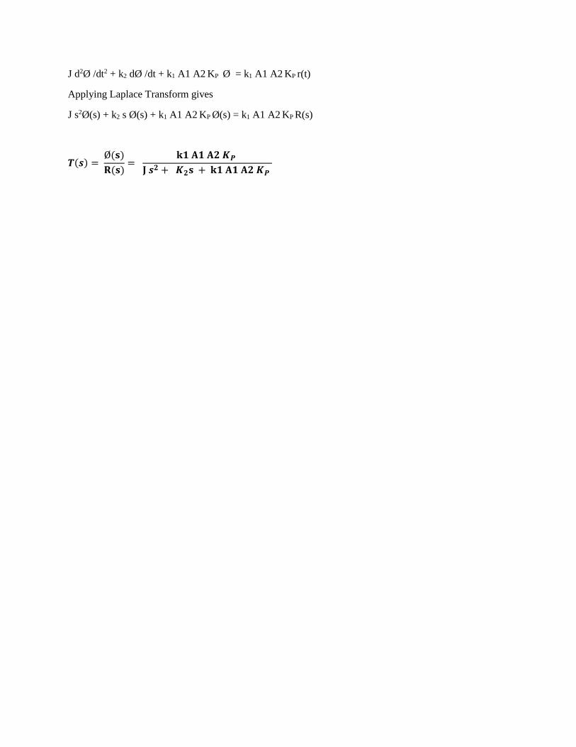
J d2Ø /dt2 + k2 dØ /dt + k1 A1 A2 KP Ø = k1 A1 A2 KP r(t)

Applying Laplace Transform gives

J s2Ø(s) + k2 s Ø(s) + k1 A1 A2 KP Ø(s) = k1 A1 A2 KP R(s)

𝑻(𝒔) = Ø(𝐬)

𝐑(𝐬)=

𝐤𝟏 𝐀𝟏 𝐀𝟐 𝑲𝑷

𝐉 𝒔𝟐 + 𝑲𝟐𝐬 + 𝐤𝟏 𝐀𝟏 𝐀𝟐 𝑲𝑷

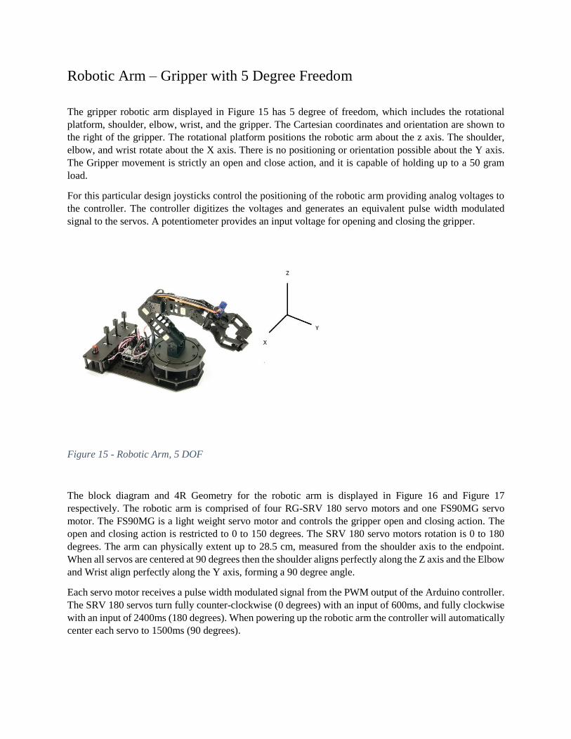
Robotic Arm – Gripper with 5 Degree Freedom

The gripper robotic arm displayed in Figure 15 has 5 degree of freedom, which includes the rotational

platform, shoulder, elbow, wrist, and the gripper. The Cartesian coordinates and orientation are shown to

the right of the gripper. The rotational platform positions the robotic arm about the z axis. The shoulder,

elbow, and wrist rotate about the X axis. There is no positioning or orientation possible about the Y axis.

The Gripper movement is strictly an open and close action, and it is capable of holding up to a 50 gram

load.

For this particular design joysticks control the positioning of the robotic arm providing analog voltages to

the controller. The controller digitizes the voltages and generates an equivalent pulse width modulated

signal to the servos. A potentiometer provides an input voltage for opening and closing the gripper.

Figure 15 - Robotic Arm, 5 DOF

The block diagram and 4R Geometry for the robotic arm is displayed in Figure 16 and Figure 17

respectively. The robotic arm is comprised of four RG-SRV 180 servo motors and one FS90MG servo

motor. The FS90MG is a light weight servo motor and controls the gripper open and closing action. The

open and closing action is restricted to 0 to 150 degrees. The SRV 180 servo motors rotation is 0 to 180

degrees. The arm can physically extent up to 28.5 cm, measured from the shoulder axis to the endpoint.

When all servos are centered at 90 degrees then the shoulder aligns perfectly along the Z axis and the Elbow

and Wrist align perfectly along the Y axis, forming a 90 degree angle.

Each servo motor receives a pulse width modulated signal from the PWM output of the Arduino controller.

The SRV 180 servos turn fully counter-clockwise (0 degrees) with an input of 600ms, and fully clockwise

with an input of 2400ms (180 degrees). When powering up the robotic arm the controller will automatically

center each servo to 1500ms (90 degrees).

The 9g servo turns fully counter-clockwise (0 degrees) with an input of 900ms, and fully clockwise with

an input of 2100ms (180 degrees). 1500ms centers the servo at 90 degrees.

Each servo can be positioned in 1 microsecond (usec) increments which translates to 0.0001 degree per 1

usec.

Degrees per usec = 180 degrees / (2,400,000 – 600,000) usec or 0.0001 degree per 1 usec.

Servo MotorRotational Platform

Z – Axis0 .. 180 deg

Servo MotorShoulder X – Axis

0 .. 180 deg

Servo MotorElbow X-Axis

0 .. 180 deg

Servo MotorWristX-Axis

0 .. 180 deg

Servo MotorGripper

Open/Close0 .. 150 deg

Controller

PWM 5

PC

USB

USB

Analog Controls

SW 1 … SW 5

PWM 4PWM 3

PWM 2PWM 1

Figure 16 - Robotic Arm, 5 DOF

Z Axis

X Axis

Angular PositionAbout Z Axis

Shoulder

Elbow

Wrist

Gripper

Figure 17 - 4R Geometry

Robotic Arm – 6 Degree Freedom

Figure 18 shows a physical view of the robotic arm with the laser mounted as an endpoint. Figure 19 and

Figure 20 show the associated block diagram and physical dimensions of the links, respectively.

Figure 18 - Robotic Arm 6 DOF and Laser Endpoint

Servo MotorRotational Position

Z – Axis0 .. 180 deg

Servo MotorShoulder - Position

X – Axis0 .. 180 deg

Servo MotorElbow - Position

X-Axis0 .. 180 deg

Servo MotorWrist Orientation

Y-Axis0 .. 180 deg

Servo MotorWrist Orientation

X-Axis0 .. 180 deg

PWM 5

PC

USB

Analog Controls

SW 1 … SW 5

PWM 4PWM 3

PWM 2PWM 1

Servo MotorWrist Orientation

Z-Axis0 .. 180 deg

PWM 6

Laser420 nm

(red)

Controller

USB

DIO 3

Figure 19 - Robotic Arm, 6 DOF

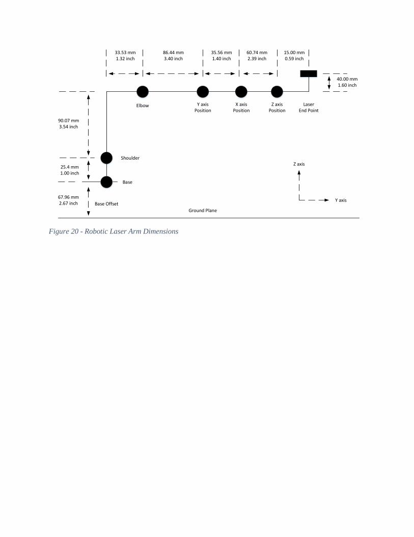
Base

25.4 mm1.00 inch

90.07 mm3.54 inch

Shoulder

Elbow

33.53 mm1.32 inch

Y axisPosition

86.44 mm3.40 inch

X axisPosition

35.56 mm1.40 inch

Z axisPosition

60.74 mm2.39 inch

15.00 mm0.59 inch

LaserEnd Point

40.00 mm1.60 inch

Ground Plane

67.96 mm2.67 inch

Z axis

Y axisBase Offset

Figure 20 - Robotic Laser Arm Dimensions

Rotation Kinematics

Read Theory of Applied Robotics, Chapter 2

Read Theory of Applied Robotics, Chapter 3

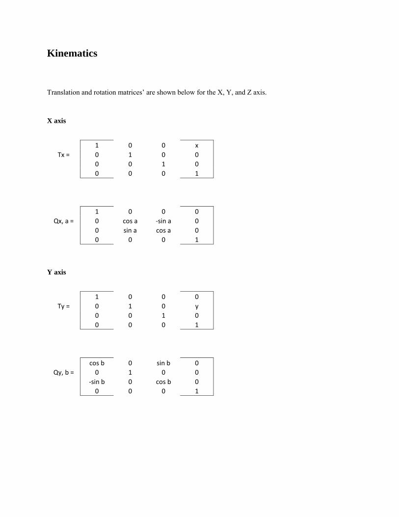
Kinematics

Translation and rotation matrices’ are shown below for the X, Y, and Z axis.

X axis

1 0 0 x

Tx = 0 1 0 0

0 0 1 0

0 0 0 1

1 0 0 0

Qx, a = 0 cos a -sin a 0

0 sin a cos a 0

0 0 0 1

Y axis

1 0 0 0

Ty = 0 1 0 y

0 0 1 0

0 0 0 1

cos b 0 sin b 0

Qy, b = 0 1 0 0

-sin b 0 cos b 0

0 0 0 1

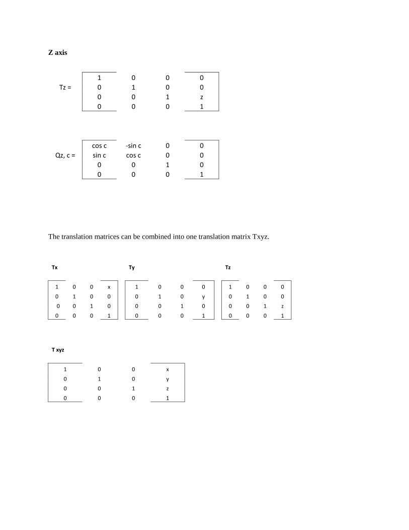
Z axis

1 0 0 0

Tz = 0 1 0 0

0 0 1 z

0 0 0 1

cos c -sin c 0 0

Qz, c = sin c cos c 0 0

0 0 1 0

0 0 0 1

The translation matrices can be combined into one translation matrix Txyz.

Tx Ty Tz

1 0 0 x 1 0 0 0 1 0 0 0

0 1 0 0 0 1 0 y 0 1 0 0

0 0 1 0 0 0 1 0 0 0 1 z

0 0 0 1 0 0 0 1 0 0 0 1

T xyz

1 0 0 x

0 1 0 y

0 0 1 z

0 0 0 1

Example:

The endpoints of a plane along the x-y axis are given below.

Z

X

Y

Points:

Pt1 Pt2 Pt3 Pt4

X 0 0 10 10

y 0 20 0 20

z 0 0 0 0

1 1 1 1

Rotate the points 30 degrees about the Z axis and then translate them two units along the Z axis.

Translation Rotation Points

Pt1 Pt2 Pt3 Pt4

1 0 0 2 cos 30 -sin 30 0 0 0 0 10 10

0 1 0 2 sin 30 cos 30 0 0 0 20 0 20

0 0 1 2 0 0 1 0 0 0 0 0

0 0 0 1 0 0 0 1 1 1 1 1

Translation Points

Pt1 Pt2 Pt3 Pt4

1 0 0 2 0 -10.00 8.66 -1.34

0 1 0 2 0 17.32 5.00 22.32

0 0 1 2 0 0.00 0.00 0.00

0 0 0 1 1 1 1 1

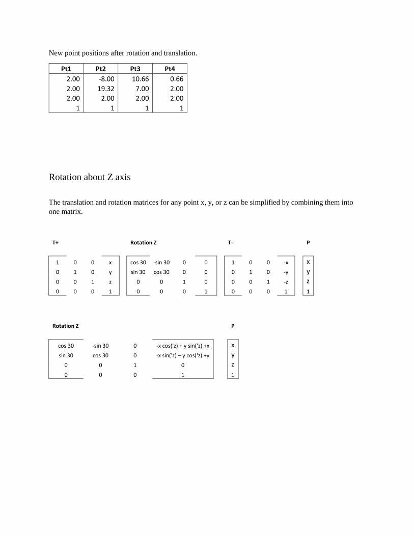
New point positions after rotation and translation.

Pt1 Pt2 Pt3 Pt4

2.00 -8.00 10.66 0.66

2.00 19.32 7.00 2.00

2.00 2.00 2.00 2.00

1 1 1 1

Rotation about Z axis

The translation and rotation matrices for any point x, y, or z can be simplified by combining them into

one matrix.

T+ Rotation Z T- P

1 0 0 x cos 30 -sin 30 0 0 1 0 0 -x x

0 1 0 y sin 30 cos 30 0 0 0 1 0 -y y

0 0 1 z 0 0 1 0 0 0 1 -z z

0 0 0 1 0 0 0 1 0 0 0 1 1

Rotation Z P

cos 30 -sin 30 0 -x cos('z) + y sin('z) +x x

sin 30 cos 30 0 -x sin('z) – y cos('z) +y y

0 0 1 0 z

0 0 0 1 1

Forward Kinematics

Read Theory of Applied Robotics, Chapter 5

Inverse Kinematics

Read Theory of Applied Robotics, Chapter 6

Software and Sketches

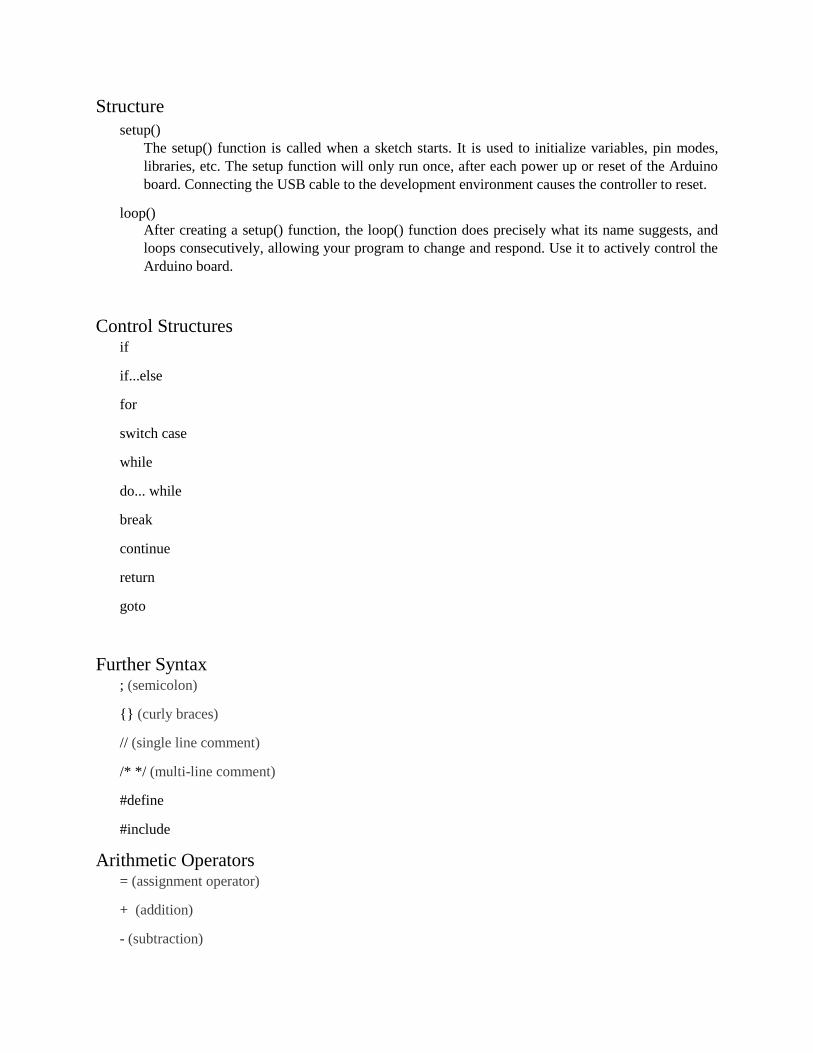
Structure

setup()

The setup() function is called when a sketch starts. It is used to initialize variables, pin modes,

libraries, etc. The setup function will only run once, after each power up or reset of the Arduino

board. Connecting the USB cable to the development environment causes the controller to reset.

loop()

After creating a setup() function, the loop() function does precisely what its name suggests, and

loops consecutively, allowing your program to change and respond. Use it to actively control the

Arduino board.

Control Structures if

if...else

for

switch case

while

do... while

break

continue

return

goto

Further Syntax ; (semicolon)

{} (curly braces)

// (single line comment)

/* */ (multi-line comment)

#define

#include

Arithmetic Operators = (assignment operator)

+ (addition)

- (subtraction)

* (multiplication)

/ (division)

% (modulo)\

Comparison Operators == (equal to)

!= (not equal to)

< (less than)

> (greater than)

<= (less than or equal to)

>= (greater than or equal to)

Boolean Operators && (and)

|| (or)

! (not)

Pointer Access Operators * dereference operator

& reference operator

Bitwise Operators & (bitwise and)

| (bitwise or)

^ (bitwise xor)

~ (bitwise not)

<< (bitshift left)

>> (bitshift right)

Compound Operators ++ (increment)

-- (decrement)

+= (compound addition)

-= (compound subtraction)

*= (compound multiplication)

/= (compound division)

&= (compound bitwise and)

|= (compound bitwise or)

Variables

Constants HIGH | LOW

INPUT | OUTPUT | INPUT_PULLUP

LED_BUILTIN

true | false

integer constants

floating point constants

Data Types void

boolean

char

unsigned char

byte

int

unsigned int

word

long

unsigned long

short

float

double

string - char array

String - object

array

Conversion char()

byte()

int()

word()

long()

float()

Variable Scope & Qualifiers variable scope

static

volatile

const

Utilities sizeof()

PROGMEM

Functions

Digital I/O pinMode()

digitalWrite()

digitalRead()

Analog I/O analogReference()

Configures the reference voltage used for analog input (i.e. the value used as the top of the input

range). The options are:

DEFAULT: the default analog reference of 5 volts (on 5V Arduino boards) or 3.3 volts (on 3.3V

Arduino boards)

INTERNAL: a built-in reference, equal to 1.1 volts on the ATmega168 or ATmega328 and 2.56

volts on the ATmega8 (not available on the Arduino Mega)

INTERNAL1V1: a built-in 1.1V reference (Arduino Mega only)

INTERNAL2V56: a built-in 2.56V reference (Arduino Mega only)

EXTERNAL: the voltage applied to the AREF pin (0 to 5V only) is used as the reference.

analogRead()

analogWrite() – PWM

Due & Zero only analogReadResolution()

analogWriteResolution()

Advanced I/O tone()

noTone()

shiftOut()

shiftIn()

pulseIn()

Time millis()

micros()

delay()

delayMicroseconds()

Math min()

max()

abs()

constrain()

map()

pow()

sqrt()

Trigonometry sin()

cos()

tan()

Random Numbers randomSeed()

random()

Bits and Bytes lowByte()

highByte()

bitRead()

bitWrite()

bitSet()

bitClear()

bit()

External Interrupts attachInterrupt()

detachInterrupt()

Interrupts interrupts()

noInterrupts()

Communication Serial

Stream

USB (32u4 based boards and Due/Zero only) Keyboard

Mouse