rna-seq analysis worksop - · pdf filerna-seq analysis worksop zhangjun fei boyce thompson...
TRANSCRIPT

RNA-seq analysis worksop
Zhangjun Fei
Boyce Thompson Institute for Plant Research
USDA Robert W. Holley Center for Agriculture and Health
Cornell University

Outline
• Background of RNA-seq
• Application of RNA-seq (what RNA-seq can do?)
• Available sequencing platforms and strategies and which one to choose
• RNA-seq data analysis
Read processing and quality assessment
De novo assembly
Alignment to reference genome/transcriptome
Differentially expressed gene identification
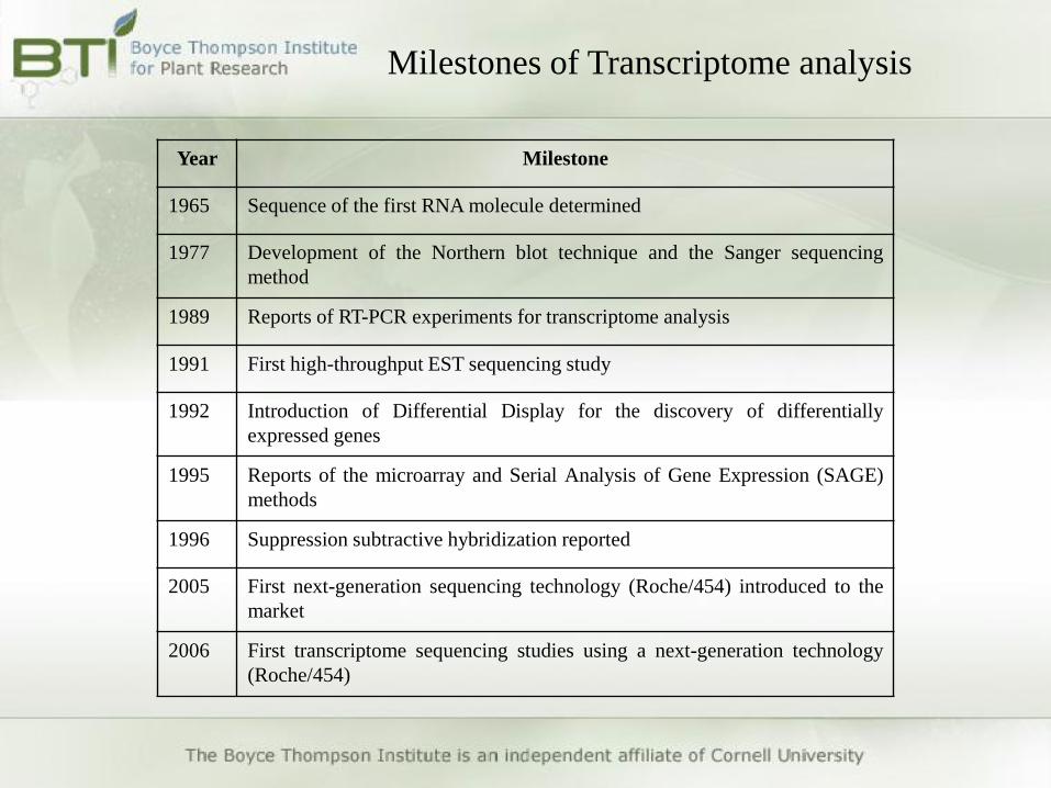
Year Milestone
1965 Sequence of the first RNA molecule determined
1977 Development of the Northern blot technique and the Sanger sequencing
method
1989 Reports of RT-PCR experiments for transcriptome analysis
1991 First high-throughput EST sequencing study
1992 Introduction of Differential Display for the discovery of differentially
expressed genes
1995 Reports of the microarray and Serial Analysis of Gene Expression (SAGE)
methods
1996 Suppression subtractive hybridization reported
2005 First next-generation sequencing technology (Roche/454) introduced to the
market
2006 First transcriptome sequencing studies using a next-generation technology
(Roche/454)
Milestones of Transcriptome analysis

New sequencing technologies
Next generation sequencing
• Pacific Biosciences
• Oxford Nanopore
• Complete Genomics
Third generation sequencing
• Illumina (HiSeq 2000/2500)
• Roche/454
• Ion Torrent (Ion Proton)
• ABI/SOLiD
• Helicos
• Ion Torrent PGM
• Illumina MiSeq
• 454 GS Junior
Desktop sequencer

RNA-seq applications
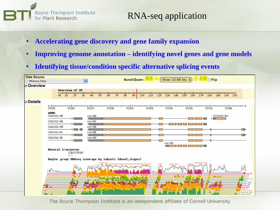
• Accelerating gene discovery and gene family expansion
• Improving genome annotation – identifying novel genes and gene models
• Identifying tissue/condition specific alternative splicing events
RNA-seq application

RNA-seq applications
• Short reads can’t provide the complete structure of an isoform
Alternative splicing

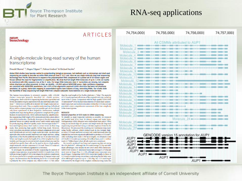
RNA-seq applications
PacBio long reads
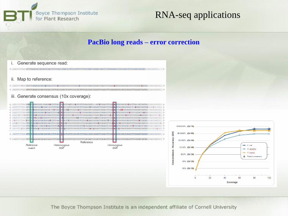
RNA-seq applications
PacBio long reads – error correction

RNA-seq applications
Each sample needs four libraries with different
insert sizes: 1-2K, 2-3K, 3-5K, >5K
RNA-seq applications

Cell 1 Cell 2
No. reads 86,126 80,543
Total base 527,933,678 476,348,201
Average length 6,129 5,914
RNA-seq applications
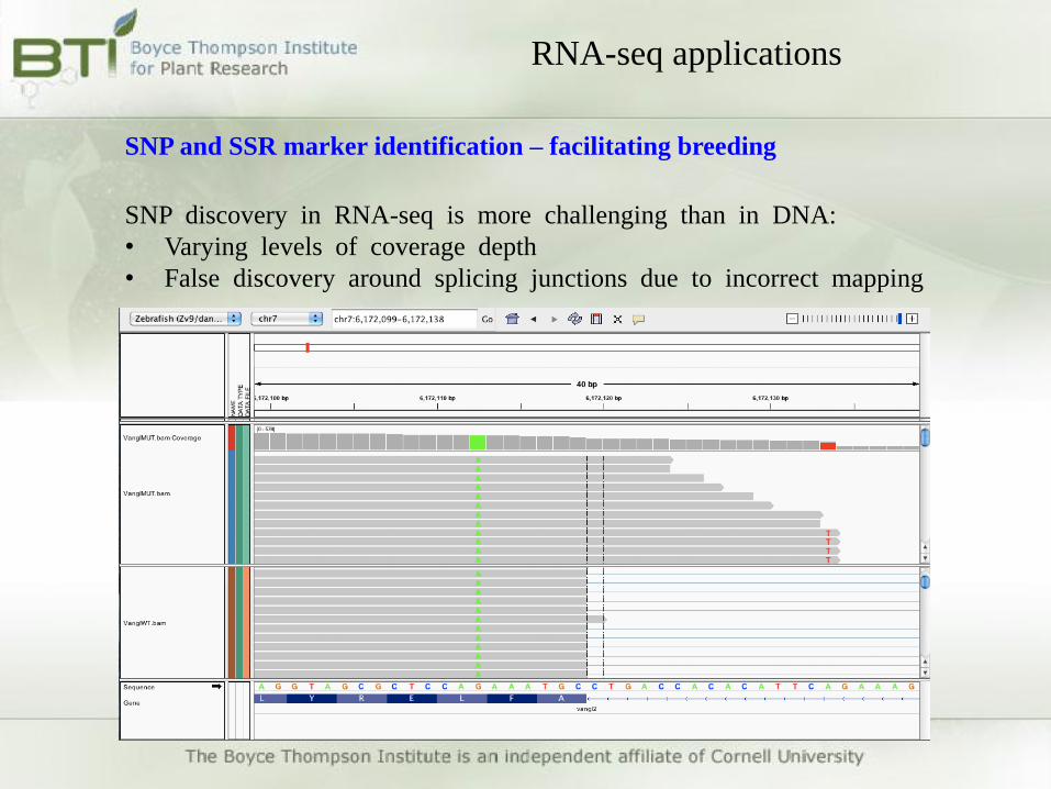
SNP discovery in RNA-seq is more challenging than in DNA:
• Varying levels of coverage depth
• False discovery around splicing junctions due to incorrect mapping
SNP and SSR marker identification – facilitating breeding
RNA-seq applications
RNA-seq applications
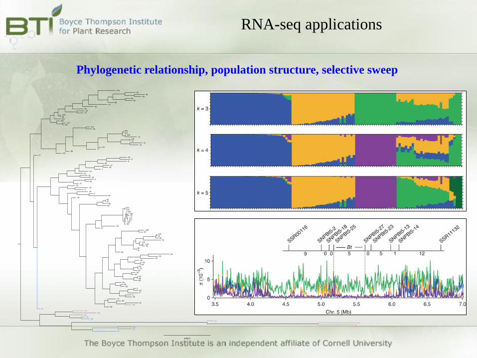
Phylogenetic relationship, population structure, selective sweep
1000.0
16
115
36
20
94
8
7
71
80
68
3
96
51
27
47
67
9
65
15
43
117
93
13
40
6
41
73
60
2
95
50
57
39
90
1
105
119
122
87
49
66
77
62
48
14
58
109
99
111
54
42
46
76
107
30
19
85
97
5
113
24
11017
112
121
11
70
25
92
83
106
26
38
18
82
35
12
23
56
64
53
102
28
22
108
32
61
55
84
75
31
37
118
72
52
59
33
101
98
104
100
114
91
116
4
74
63
81
29
45
10
79
120
103
44
78
86
34
69
21
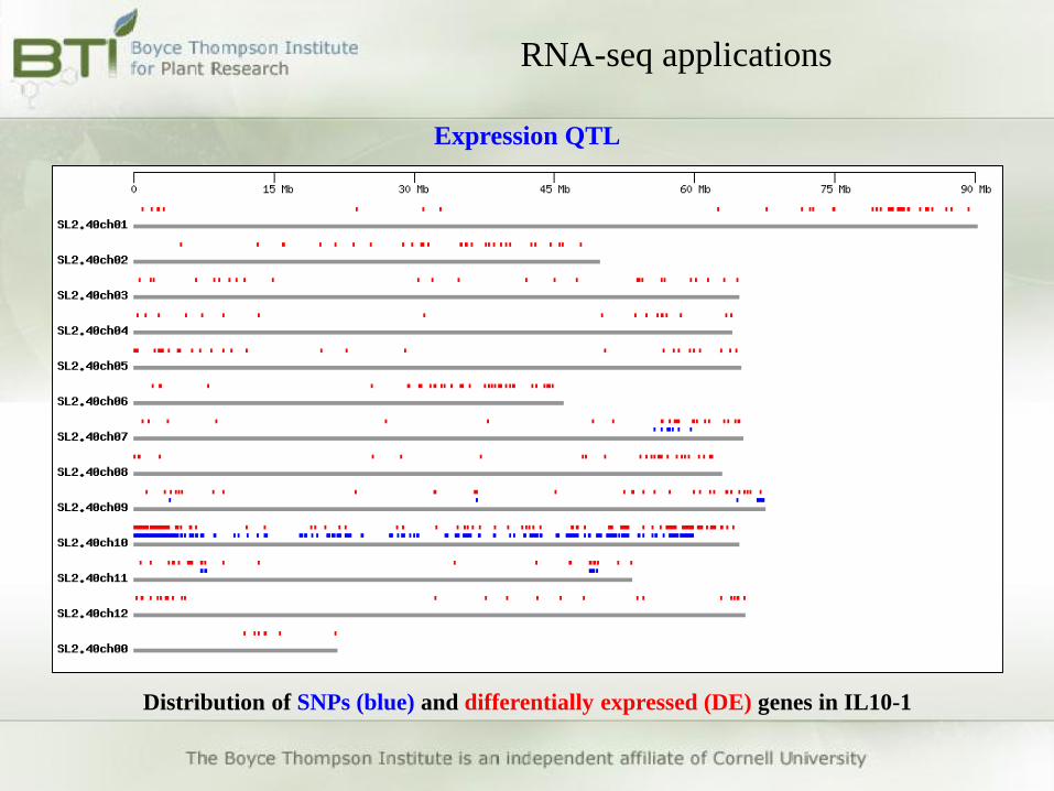
Distribution of SNPs (blue) and differentially expressed (DE) genes in IL10-1
Expression QTL
RNA-seq applications

Mutant gene cloning (BSA RNA-seq)
white fruit x yellow fruit
F1
F2
F3
yellow poolwhite pool
RNA-seq
SNPs and DE genes
132 of 189 SNPs in this region
RNA-seq applications
kb

Distribution of mapped markers associating with the
erucic acid trait
GWAS
RNA-seq applications

Genomic imprinting and allele specific expression
RNA-seq applications

non-coding RNAs (lncRNA, lincRNAs…)
RNA-seq applications
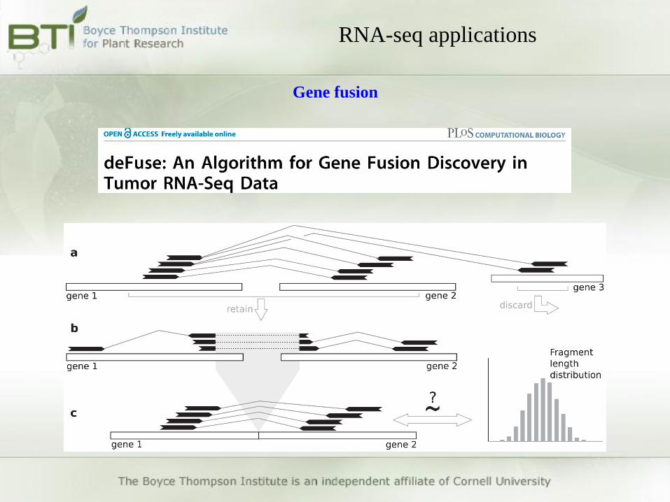
Gene fusion
RNA-seq applications

RNA-seq applications
Gene expression profiling

• Cross-hybridization
• Stable probe secondary structures
• high background (e.g., nonspecific hybridization)
• limited dynamic range (e.g., nonlinear and saturable hybridization
kinetics)
• allow direct enumeration of transcript molecules
• digital expression data are absolute so data can be directly
compared across different experiments and laboratories without
the need for extensive internal controls or other experimental
manipulation
• provide open systems that allow detection of previously
uncharacterized transcripts, as well as rare transcripts
Problem of microarray
RNA-seq (digital expression analysis)
RNA-seq vs microarray
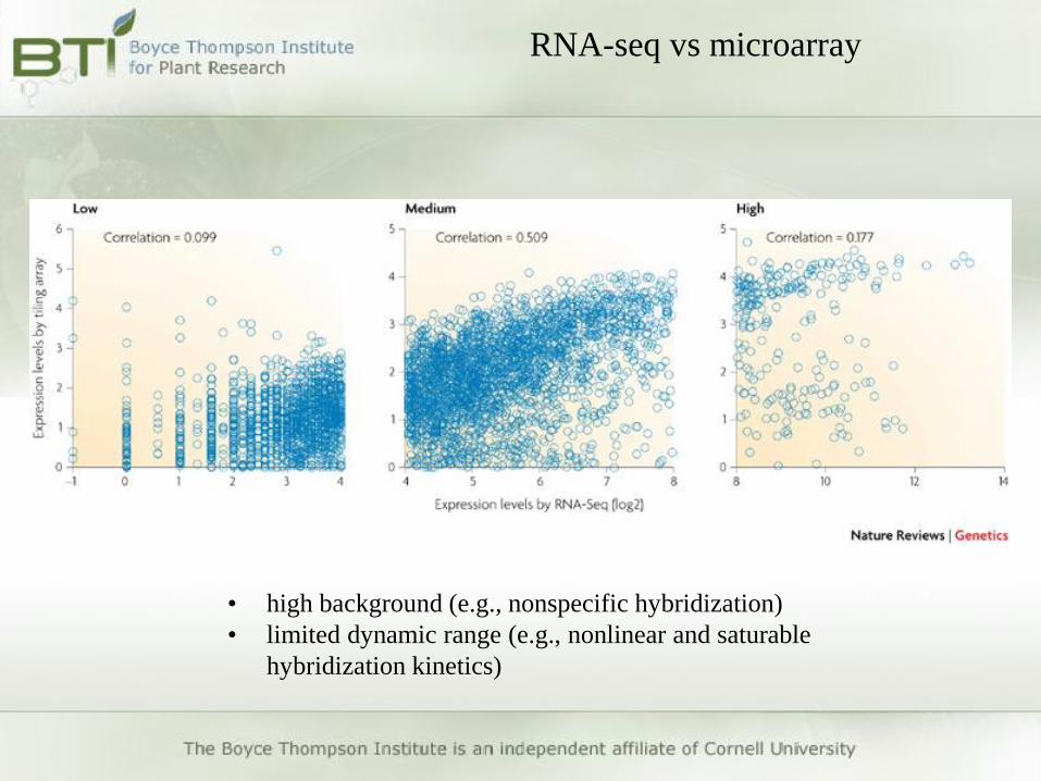
RNA-seq vs microarray
• high background (e.g., nonspecific hybridization)
• limited dynamic range (e.g., nonlinear and saturable
hybridization kinetics)

RNA-seq applications
Summary
Accelerating gene discovery and gene family expansion
Improving genome annotation – identifying novel genes and gene models
Identifying tissue/condition specific alternative splicing events
SNP and SSR marker identification
Phylogenetic relationship, population structure, selective sweep
Expression QTL analysis
Mutant gene cloning (BSA RNA-seq)
Genome (Transcriptome)-wide associate study
Genomic imprinting and allele specific expression analysis
Identifying non-coding RNAs (lncRNA, lincRNAs…)
Identifying gene fusion events
Gene expression profiling analysis

Sequencing platforms and strategies
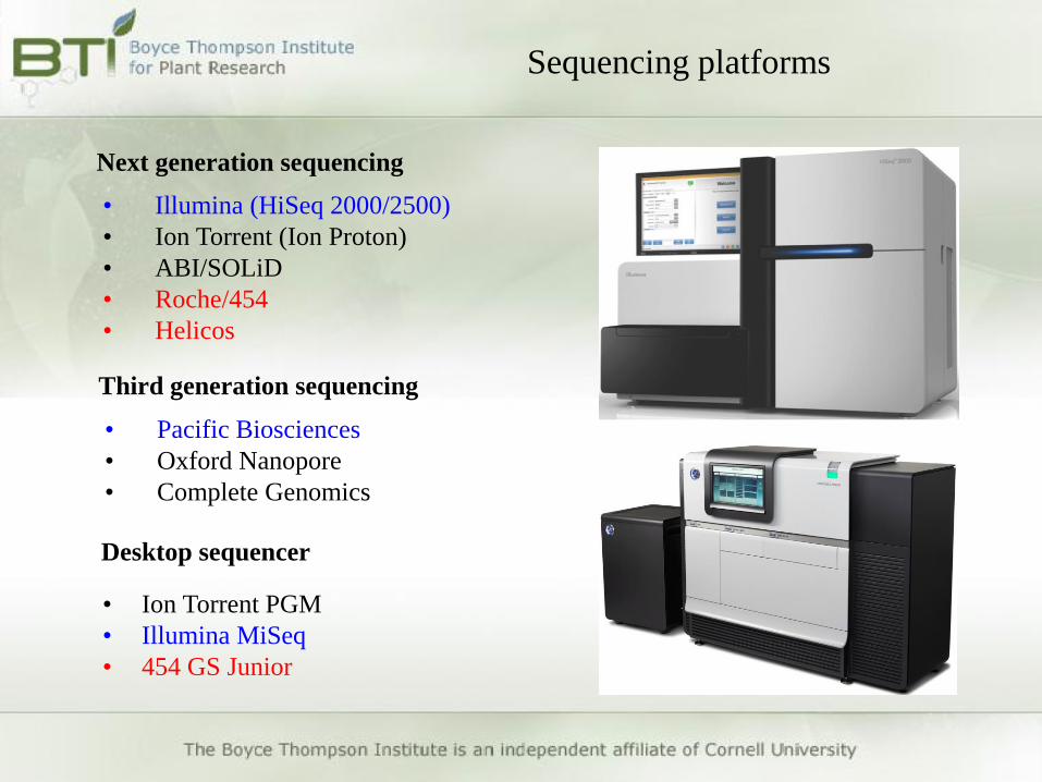
Sequencing platforms
Next generation sequencing
• Pacific Biosciences
• Oxford Nanopore
• Complete Genomics
Third generation sequencing
• Illumina (HiSeq 2000/2500)
• Ion Torrent (Ion Proton)
• ABI/SOLiD
• Roche/454
• Helicos
• Ion Torrent PGM
• Illumina MiSeq
• 454 GS Junior
Desktop sequencer

http://www.biotech.cornell.edu/brc/genomics/services/price-list
High-output mode (150-200M reads/
read pairs per lane)
Single-end, 50 bp lane
Single-end, 100 bp lane
Paired-end, 2 x 100bp lane
Run time: 2-11 days
Rapid run mode (100-150M reads/
read pairs per lane)
Single-end, 50 bp lane
Single-end, 100 bp lane
Paired-end, 2 x 100bp lane
Paired-end, 2 x 150bp lane
Runtime: 7-40 hours
50 bp sequencing kit
300 bp sequencing kit (e.g. 2 x 150 bp)
500 bp sequencing kit (e.g. 2 x 250 bp)
150 bp sequencing kit (e.g. 2 x 75 bp)
600 bp sequencing kit (e.g. 2 x 300 bp)
Run time: 5-65 hours
Illumina HiSeq 2000/2500 Illumina MiSeq
Sequencing platforms
Sequencing platforms
Single-end or paired-end
For gene expression analysis with a reference genome, single-
end is enough
For de novo assembly, genome annotation, alternative splicing
identification……, it’s better to use paired-end
Strand-specific or non strand-specific
Always choose strand-specific RNA-seq if possible

Strand-specific RNA sequencing
• More accurately determine the expression level
• Significantly reduce false positives in identifying alternatively
spliced transcripts
• Identify antisense transcripts – another level of gene regulation
in important biological processes
• Determine the transcribed strand of non-coding RNAs (e.g.
lincRNAs)

Strand-specific RNA-seq library construction

Up to 96 libraries in two days
Paired-end compatible
multiplexing
High throughput ssRNA-seq
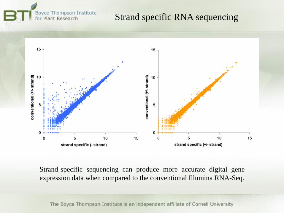
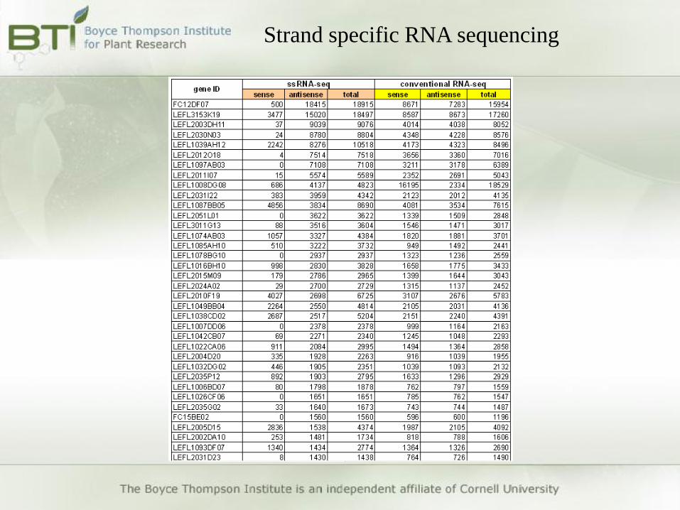
Strand specific RNA sequencing
Strand-specific sequencing can produce more accurate digital gene
expression data when compared to the conventional Illumina RNA-Seq.
Strand specific RNA sequencing

Strand specific RNA sequencing
Antisense transcript
cis-natural antisense transcripts (cis-NAT)
1340 cis-NAT pairs in Arabidopsis (Wang et al., 2005)
687 cis-NAT pairs in rice (Osato et al., 2003)
trans-natural antisense transcripts (trans-NAT)
1,320 trans-NAT pairs in Arabidopsis (Wang et al., 2006)
alternative splicing
RNA editing
DNA methylation
genomic imprinting
X-chromosome inactivation
function
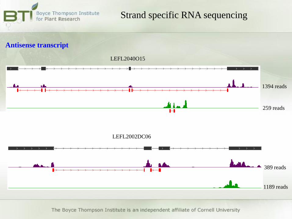
LEFL2040O15
1394 reads
259 reads
LEFL2002DC06
1189 reads
389 reads
Strand specific RNA sequencing
Antisense transcript
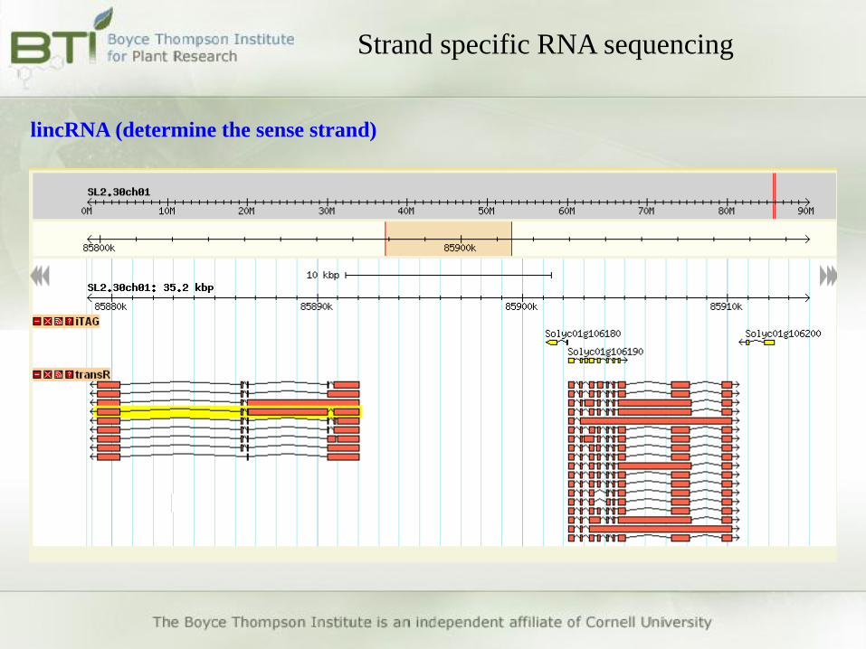
Strand specific RNA sequencing
lincRNA (determine the sense strand)

RNA-seq strategies
Most frequently asked question
• “How many samples should I multiplex in one lane?” or “How many reads
should I generate for each of my samples?”
• Depend on $$$
• Depends on the quality of the library and the reads
rRNA, tRNA, organelle, adaptor contamination
• No. of biological replicates for expression call
At least three
• Effects of read numbers on expression call
Mature green fruit library (22M reads)
Randomly select 0.1-0.9, 1-22M reads from the library and calculate
gene expression for each dataset (20 different randomizations)
Sequencing depth and no. of biological replicates
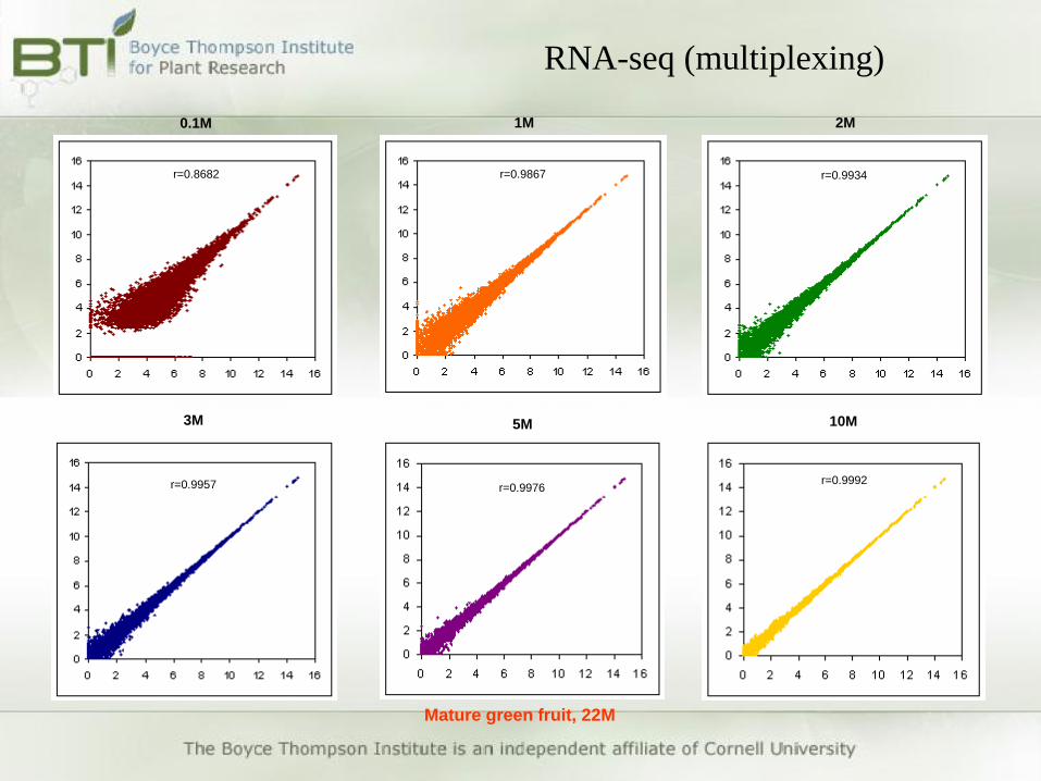
RNA-seq (multiplexing)
r=0.9867
r=0.9992r=0.9976
r=0.9934
r=0.9957
r=0.8682
0.1M 1M 2M
3M 5M 10M
Mature green fruit, 22M

RNA-seq (multiplexing)

RNA-seq (multiplexing)

RNA-seq data analysis

Read quality control (fastqc)
Read processing

Read processing
Read quality control (fastqc)

Read processing
Read quality control (fastqc)
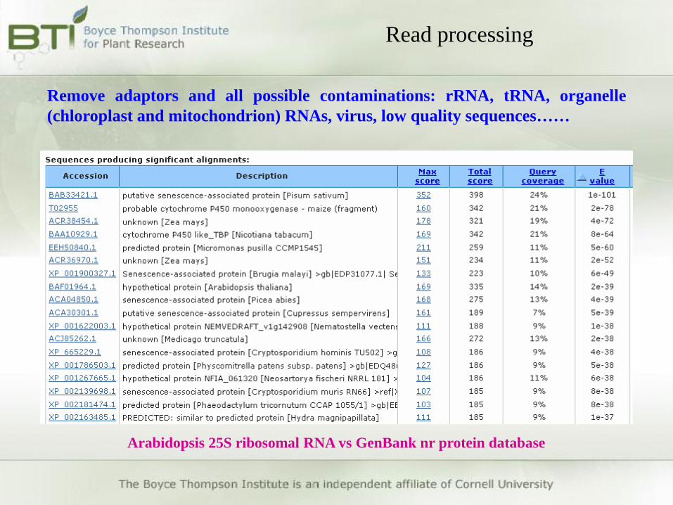
Remove adaptors and all possible contaminations: rRNA, tRNA, organelle
(chloroplast and mitochondrion) RNAs, virus, low quality sequences……
Arabidopsis 25S ribosomal RNA vs GenBank nr protein database
Read processing

Remove contaminated sequences
• Align reads to rRNA and organelle
sequence database (bowtie or BWA)
• Affect RPKM values if not removed
Trim adaptor and low quality sequences
• FASTX-Toolkit
• AdapterRemoval
• Trimmomatic
• Cutadapt
• Condetri
• ERNE-filter
• Prinseq
• SolexaQA-bwa
• Sickle
Read processing

Read processing
RNA-seq data analysis
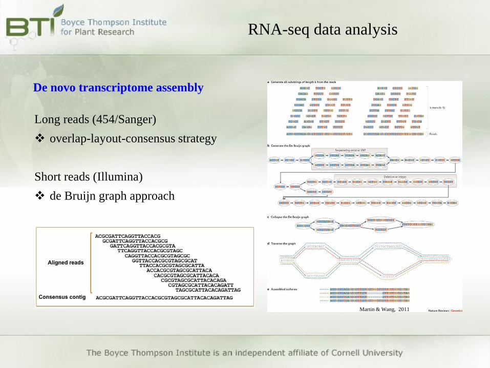
De novo transcriptome assembly
Long reads (454/Sanger)
overlap-layout-consensus strategy
Short reads (Illumina)
de Bruijn graph approach
Martin & Wang, 2011
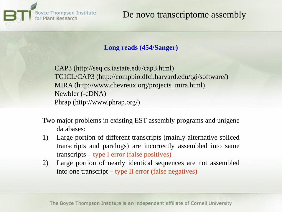
Two major problems in existing EST assembly programs and unigene
databases:
1) Large portion of different transcripts (mainly alternative spliced
transcripts and paralogs) are incorrectly assembled into same
transcripts – type I error (false positives)
2) Large portion of nearly identical sequences are not assembled
into one transcript – type II error (false negatives)
De novo transcriptome assembly
CAP3 (http://seq.cs.iastate.edu/cap3.html)
TGICL/CAP3 (http://compbio.dfci.harvard.edu/tgi/software/)
MIRA (http://www.chevreux.org/projects_mira.html)
Newbler (-cDNA)
Phrap (http://www.phrap.org/)
Long reads (454/Sanger)
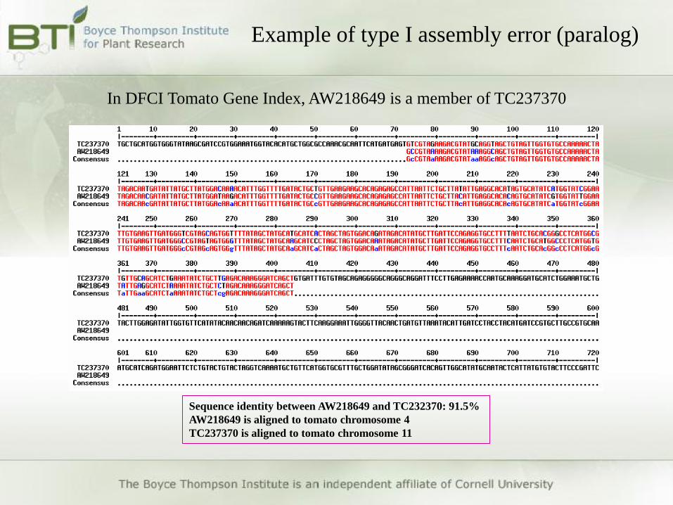
Example of type I assembly error (paralog)
In DFCI Tomato Gene Index, AW218649 is a member of TC237370
Sequence identity between AW218649 and TC232370: 91.5%
AW218649 is aligned to tomato chromosome 4
TC237370 is aligned to tomato chromosome 11
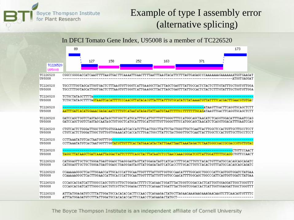
Example of type I assembly error
(alternative splicing)
In DFCI Tomato Gene Index, U95008 is a member of TC226520

Example of type II assembly error
In DFCI Tomato Gene Index, two unigenes, TC219875 and TC221582, are identical
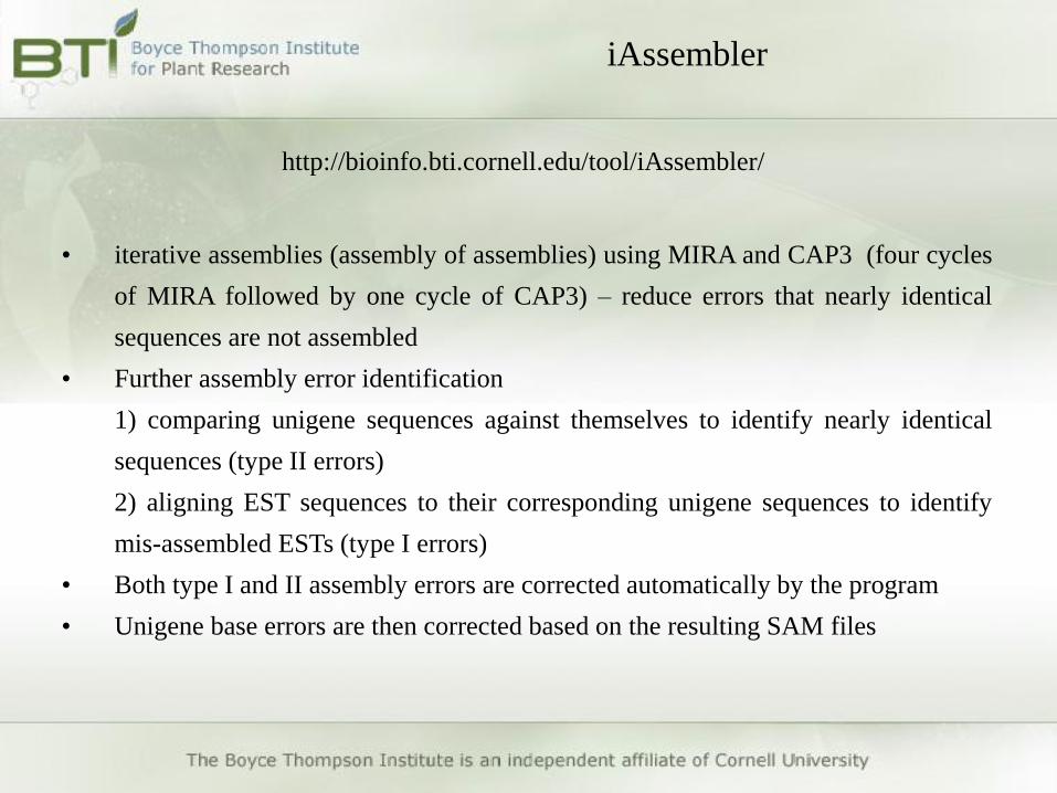
iAssembler
http://bioinfo.bti.cornell.edu/tool/iAssembler/
• iterative assemblies (assembly of assemblies) using MIRA and CAP3 (four cycles
of MIRA followed by one cycle of CAP3) – reduce errors that nearly identical
sequences are not assembled
• Further assembly error identification
1) comparing unigene sequences against themselves to identify nearly identical
sequences (type II errors)
2) aligning EST sequences to their corresponding unigene sequences to identify
mis-assembled ESTs (type I errors)
• Both type I and II assembly errors are corrected automatically by the program
• Unigene base errors are then corrected based on the resulting SAM files
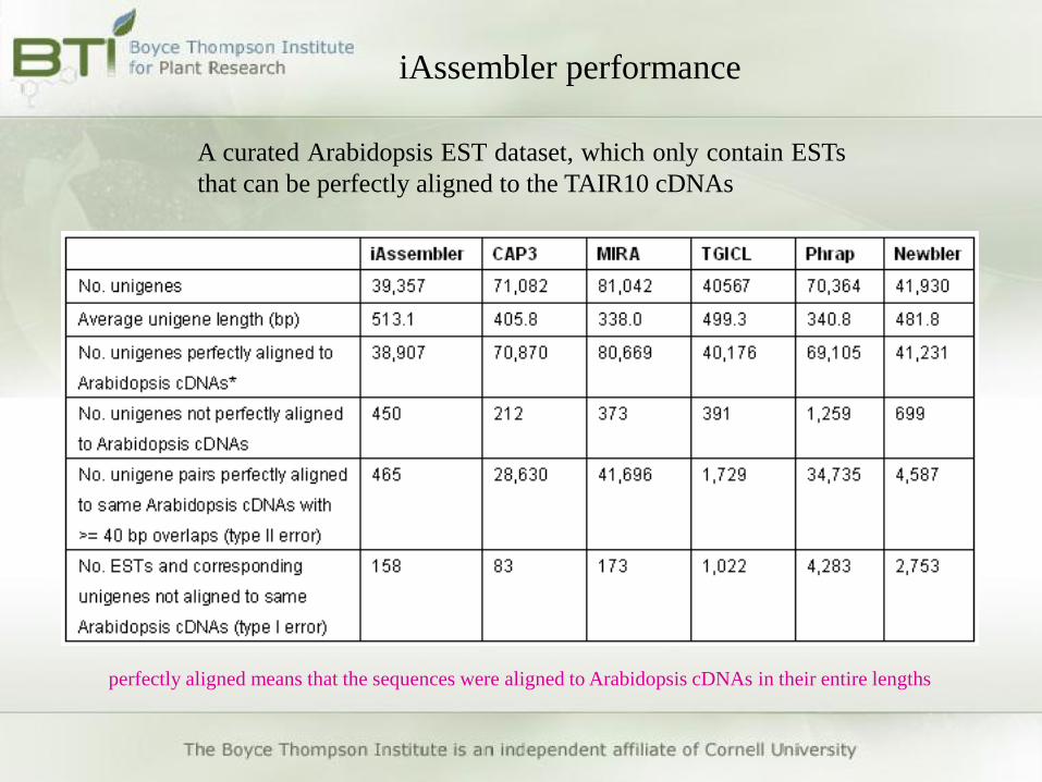
iAssembler performance
A curated Arabidopsis EST dataset, which only contain ESTs
that can be perfectly aligned to the TAIR10 cDNAs
perfectly aligned means that the sequences were aligned to Arabidopsis cDNAs in their entire lengths

Trinity
Trans-ABySS
Oases/velvet
SOAPdenovo-Trans
De novo transcriptome assembly
Short reads (Illumina)
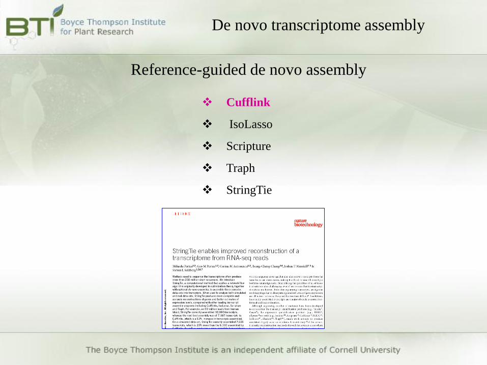
De novo transcriptome assembly
Reference-guided de novo assembly
Cufflink
IsoLasso
Scripture
Traph
StringTie

De novo transcriptome assembly
Trinity
De novo transcriptome assembly
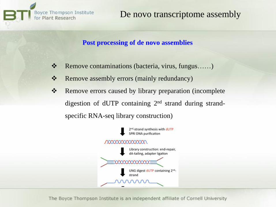
Post processing of de novo assemblies
Remove contaminations (bacteria, virus, fungus……)
Remove assembly errors (mainly redundancy)
Remove errors caused by library preparation (incomplete
digestion of dUTP containing 2nd strand during strand-
specific RNA-seq library construction)

De novo transcriptome assembly
Remove contamination
blastn
blastx

De novo transcriptome assembly
DeconSeq
SeqClean
Remove contamination
De novo transcriptome assembly
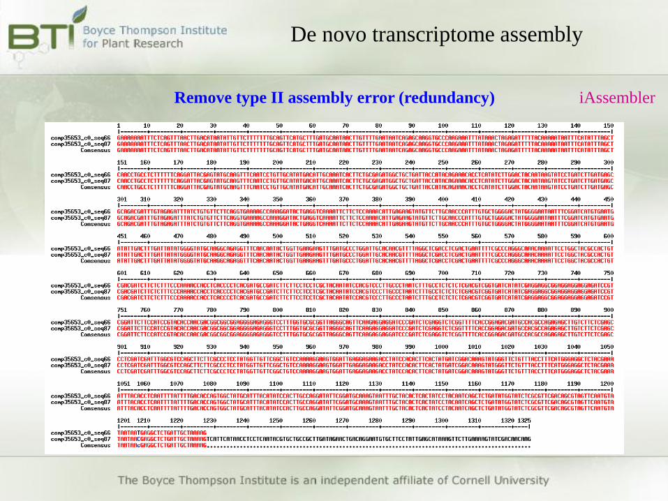
Remove type II assembly error (redundancy) iAssembler

Gene ID length antisense sense
UN22492 1504 97 48138
comp38294_c0_seq1 526 10822 103
De novo transcriptome assembly
Remove transcripts derived from incomplete 2nd digestion
removed

De novo transcriptome assembly
High number of assembled transcripts
Alternative splicing
Non-coding RNAs
Incomplete coverage of full length transcripts
DFCI gene index

RNA-seq data analysis
Alignment
Align reads to reference genome
TopHat
HISAT
Alignment reads to reference transcriptome
bowtie
BWA
If you have a reference genome, it’s not a good
idea to align the reads to the predicted CDS or
cDNA, due to the incomplete prediction of UTRs
and alternative splicing

Visualization tools
RNA-seq data analysis
Integrative Genomics Viewer (IGV)

RNA-seq data analysis
Read counting and normalization
Read counting
htseq-count
samtools (samtools view –c)
Normalization
RPKM: reads per kilobase of exon model per
million mapped reads
FPKM: fragments per kilobase of exon model per
million mapped reads

Sample correlation matrix
Quality control – biological replicates
RNA-seq data analysis
RNA-seq data analysis
Differentially expressed gene detection
Pair-wise comparison
DESeq
edgeR
Time course data
first data transformation using getVarianceStabilizedData
function in DESeq (to get normal distribution). Then DE
gene identification using F tests in LIMMA
Multiple test correction
False Discovery Rate (FDR)
q value

RNA-seq data analysis
Differentially expressed gene detection