response of stream chemistry during base flow to - usgs
TRANSCRIPT

U.S. Department of the InteriorU.S. Geological Survey
Scientific Investigations Report 2007–5083
National Water-Quality Assessment Program
Response of Stream Chemistry During Base Flow toGradients of Urbanization in Selected LocationsAcross the Conterminous United States, 2002–04

Response of Stream Chemistry During Base Flow to Gradients of Urbanization in Selected Locations Across the Conterminous United States, 2002–04
By Lori A. Sprague, Douglas A. Harned, David W. Hall, Lisa H. Nowell, Nancy J. Bauch, and Kevin D. Richards
National Water-Quality Assessment Program
Scientific Investigations Report 2007–5083
U.S. Department of the InteriorU.S. Geological Survey

U.S. Department of the InteriorDIRK KEMPTHORNE, Secretary
U.S. Geological SurveyMark D. Myers, Director
U.S. Geological Survey, Reston, Virginia: 2007
For product and ordering information: World Wide Web: http://www.usgs.gov/pubprod Telephone: 1-888-ASK-USGS
For more information on the USGS--the Federal source for science about the Earth, its natural and living resources, natural hazards, and the environment: World Wide Web: http://www.usgs.gov Telephone: 1-888-ASK-USGS
Any use of trade, product, or firm names is for descriptive purposes only and does not imply endorsement by the U.S. Government.
Although this report is in the public domain, permission must be secured from the individual copyright owners to reproduce any copyrighted materials contained within this report.
Suggested citation:Sprague, L.A., Harned, D.A., Hall, D.W., Nowell, L.H., Bauch, N.J., and Richards, K.D., 2007, Response of stream chemistry during base flow to gradients of urbanization in selected locations across the conterminous United States, 2002–04: U.S. Geological Survey Scientific Investigations Report 2007–5083, 133 p.

iii
Foreword
The U.S. Geological Survey (USGS) is committed to providing the Nation with credible scientific information that helps to enhance and protect the overall quality of life and that facilitates effective management of water, biological, energy, and mineral resources (http://www.usgs.gov/). Information on the Nation’s water resources is critical to ensuring long-term availability of water that is safe for drinking and recreation and is suitable for industry, irrigation, and fish and wildlife. Population growth and increasing demands for water make the availability of that water, now measured in terms of quantity and quality, even more essential to the long-term sustainability of our communities and ecosystems.
The USGS implemented the National Water-Quality Assessment (NAWQA) Program in 1991 to support national, regional, State, and local information needs and decisions related to water-quality management and policy (http://water.usgs.gov/nawqa). The NAWQA Program is designed to answer: What is the condition of our Nation’s streams and ground water? How are conditions changing over time? How do natural features and human activities affect the quality of streams and ground water, and where are those effects most pronounced? By combining information on water chemistry, physical characteristics, stream habitat, and aquatic life, the NAWQA Program aims to provide science-based insights for current and emerging water issues and priorities. From 1991–2001, the NAWQA Program completed interdisciplinary assessments and established a baseline understanding of water-quality conditions in 51 of the Nation’s river basins and aquifers, referred to as Study Units (http://water.usgs.gov/nawqa/studyu.html).
Multiple national and regional assessments are ongoing in the second decade (2001–2012) of the NAWQA Program as 42 of the 51 Study Units are reassessed. These assessments extend the findings in the Study Units by determining status and trends at sites that have been consis-tently monitored for more than a decade, and filling critical gaps in characterizing the quality of surface water and ground water. For example, increased emphasis has been placed on assess-ing the quality of source water and finished water associated with many of the Nation’s largest community water systems. During the second decade, NAWQA is addressing five national priority topics that build an understanding of how natural features and human activities affect water quality, and establish links between sources of contaminants, the transport of those con-taminants through the hydrologic system, and the potential effects of contaminants on humans and aquatic ecosystems. Included are topics on the fate of agricultural chemicals, effects of urbanization on stream ecosystems, bioaccumulation of mercury in stream ecosystems, effects of nutrient enrichment on aquatic ecosystems, and transport of contaminants to public-supply wells. These topical studies are conducted in those Study Units most affected by these issues; they comprise a set of multi-Study-Unit designs for systematic national assessment. In addition, national syntheses of information on pesticides, volatile organic compounds (VOCs), nutrients, selected trace elements, and aquatic ecology are continuing.
The USGS aims to disseminate credible, timely, and relevant science information to address practical and effective water-resource management and strategies that protect and restore water quality. We hope this NAWQA publication will provide you with insights and information to meet your needs, and will foster increased citizen awareness and involvement in the protec-tion and restoration of our Nation’s waters.

iv
The USGS recognizes that a national assessment by a single program cannot address all water-resource issues of interest. External coordination at all levels is critical for cost-effective man-agement, regulation, and conservation of our Nation’s water resources. The NAWQA Program, therefore, depends on advice and information from other agencies—Federal, State, regional, interstate, Tribal, and local—as well as nongovernmental organizations, industry, academia, and other stakeholder groups. Your assistance and suggestions are greatly appreciated.
Robert M. Hirsch Associate Director for Water

v
Contents
Abstract ...........................................................................................................................................................1Introduction.....................................................................................................................................................2
Background............................................................................................................................................2Nutrients ........................................................................................................................................2Pesticides ......................................................................................................................................3Suspended Sediment ..................................................................................................................3Sulfate and Chloride ....................................................................................................................3
NAWQA study on the Effects of Urbanization on Stream Ecosystems ........................................4Purpose and Scope ..............................................................................................................................4Description of the Study Areas ..........................................................................................................4
Atlanta ...........................................................................................................................................5Raleigh-Durham ...........................................................................................................................5Milwaukee-Green Bay ................................................................................................................6Dallas-Fort Worth .........................................................................................................................6Denver ...........................................................................................................................................7Portland .........................................................................................................................................7
Acknowledgments ................................................................................................................................7Approach .........................................................................................................................................................7
Geographic Information System Data ...............................................................................................7Site Selection.........................................................................................................................................8
Variability in Natural Landscape Features ..............................................................................8Gradient in the Degree of Urbanization ...................................................................................9
Data Collection ......................................................................................................................................9Environmental Samples ..............................................................................................................9Quality-Control Samples ...........................................................................................................10
Data Analysis .......................................................................................................................................10Data Compilation ........................................................................................................................10Quality-Control Analysis ...........................................................................................................14Patterns of Response to Urbanization ...................................................................................14Benchmark Exceedances ........................................................................................................24
Human-Health and Drinking-Water Benchmarks .......................................................24Aquatic-Life Benchmarks ................................................................................................25
Ambient Water-Quality Criteria for Aquatic Organisms ....................................25Toxicity Values from Pesticide Risk Assessments .............................................25
Ecoregional Nutrient Criteria .........................................................................................26Response of Stream Chemistry to Gradients of Urbanization ..............................................................26
Patterns of Response to Urbanization .............................................................................................27Nutrients ......................................................................................................................................27
Nitrogen ..............................................................................................................................27Phosphorus ........................................................................................................................29
Pesticides ....................................................................................................................................30Total Herbicide Concentrations ......................................................................................30
vi
Total Insecticide Concentrations ...................................................................................37Individual Pesticide Detections and Pesticide Toxicity Index ...................................38
Suspended Sediment ................................................................................................................52Sulfate .........................................................................................................................................52Chloride........................................................................................................................................61Comparison of the patterns of response to urbanization among study areas ................62
Benchmark Exceedances .................................................................................................................63Nutrients, pH, Sulfate, and Chloride .......................................................................................63Pesticides ....................................................................................................................................63
Summary........................................................................................................................................................66References Cited..........................................................................................................................................68Appendix 1. Seasonal response of base-flow chemistry to urbanization ......................................78Appendix 2. Quality-control data: 2a. Concentrations in blank samples ..........................................................................88 2b. Relative percent difference between replicate samples ..................................96 2c. Percent recovery of spiked pesticide compounds ...........................................106Appendix 3. Water-quality benchmarks for nutrients, sulfate, chloride, and pH ........................114Appendix 4. Water-quality benchmarks for pesticide compounds ................................................116Appendix 5. Site-specific exceedances of water-quality benchmarks ........................................121
Figures 1. Location of the study areas.........................................................................................................5 2. Land cover for basins in the Atlanta, Raleigh-Durham, Milwaukee-Green Bay, Dallas-Fort Worth, Denver, and Portland study areas, 2001. ..........................................6 3. (A) Total nitrogen, (B) dissolved nitrate, (C) total phosphorus, and (D) dissolved orthophosphate concentrations during high and low base flow compared to the percentage of urban land cover in the basin in the Atlanta, Raleigh-Durham, Milwaukee-Green Bay, Dallas-Fort Worth, Denver,
and Portland study areas ...................................................................................................28 4. (A) Total herbicide and (B) total insecticide concentrations during high and low base flow compared to the percentage of urban land cover in the basin in the Atlanta, Raleigh-Durham, Milwaukee-Green Bay, Dallas-Fort Worth, Denver, and Portland study areas ...................................................31 5. Pesticide concentrations (A) measured in stream water, (B) normalized by the cladoceran pesticide toxicity index, and (C) normalized by the fish pesticide toxicity index during high base-flow conditions compared to the percentage of urban land cover in the basin in the Atlanta study area ..............39 6. Pesticide concentrations (A) measured in stream water, (B) normalized by the cladoceran pesticide toxicity index, and (C) normalized by the fish pesticide toxicity index during low base-flow conditions compared to the percentage of urban land cover in the Atlanta study area ....................................40

vii
7. Pesticide concentrations (A) measured in stream water, (B) normalized by the cladoceran pesticide toxicity index, and (C) normalized by the fish pesticide toxicity index during high base-flow conditions compared to the percentage of urban land cover in the Raleigh-Durham study area ...............41 8. Pesticide concentrations (A) measured in stream water, (B) normalized by the cladoceran pesticide toxicity index, and (C) normalized by the fish pesticide toxicity index during low base-flow conditions compared to the percentage of urban land cover in the basin in the Raleigh-Durham study area .............................................................................................................................42 9. Pesticide concentrations (A) measured in stream water, (B) normalized by the cladoceran pesticide toxicity index, and (C) normalized by the fish pesticide toxicity index during high base-flow conditions compared to the percentage of urban land cover in the basin in the Milwaukee-Green Bay study area ....................................................................................43 10. Pesticide concentrations (A) measured in stream water, (B) normalized by the cladoceran pesticide toxicity index, and (C) normalized by the fish pesticide toxicity index during low base-flow conditions compared to the percentage of urban land cover in the basin in the Milwaukee-Green Bay study area ...............44 11. Pesticide concentrations (A) measured in stream water, (B) normalized by the cladoceran pesticide toxicity index, and (C) normalized by the fish pesticide toxicity index during high base-flow conditions compared to the percentage of urban land cover in the basin in the Dallas-Fort Worth study area .................................................................................................................45 12. Pesticide concentrations (A) measured in stream water, (B) normalized by the cladoceran pesticide toxicity index, and (C) normalized by the fish pesticide toxicity index during low base-flow conditions compared to the percentage of urban land cover in the basin in the Dallas-Fort Worth study area .................................................................................................................46 13. Pesticide concentrations (A) measured in stream water, (B) normalized by the cladoceran pesticide toxicity index, and (C) normalized by the fish pesticide toxicity index during high base-flow conditions compared to the percentage of urban land cover in the basin in the Denver study area ..........................................47 14. Pesticide concentrations (A) measured in stream water, (B) normalized by the cladoceran pesticide toxicity index, and (C) normalized by the fish pesticide toxicity index during low base-flow conditions compared to the percentage of urban land cover in the basin in the Denver study area ..............48 15. Pesticide concentrations (A) measured in stream water, (B) normalized by the cladoceran pesticide toxicity index, and (C) normalized by the fish pesticide toxicity index during high base-flow conditions compared to the percentage of urban land cover in the basin in the Portland study area .............................................................................................................................49

viii
16. Pesticide concentrations (A) measured in stream water, (B) normalized by the cladoceran pesticide toxicity index, and (C) normalized by the fish pesticide toxicity index during low base-flow conditions compared to the percentage of urban land cover in the basin in the Portland study area .............................................................................................................................50 17. (A) Suspended-sediment, (B) dissolved sulfate, and (C) dissolved chloride concentrations during high and low base flow compared to the percentage of urban land cover in the basin in the Atlanta, Raleigh-Durham, Milwaukee-Green Bay, Dallas-Fort Worth, Denver, and Portland study areas ........53 18. The number and type of benchmark exceedances for all constituents combined in the Atlanta, Raleigh-Durham, Milwaukee-Green Bay, Dallas-Fort Worth, Denver, and Portland study areas. ..................................................65
Appendix 1 Figure 1.1. Bimonthly total nitrogen concentrations compared to the percentage of urban land cover in the basin ...................................................................................79Figure 1.2. Bimonthly dissolved nitrate concentrations compared to the percentage of urban land cover in the basin ...............................................................80 Figure 1.3. Bimonthly total phosphorus concentrations compared to the percentage of urban land cover in the basin. ...............................................................81Figure 1.4. Bimonthly dissolved orthophosphate concentrations compared to the percentage of urban land cover in the basin ....................................................82Figure 1.5. Bimonthly total herbicide concentrations compared to the percentage of urban land cover in the basin ................................................................83Figure 1.6. Bimonthly total insecticide concentrations compared to the percentage of urbanland cover in the basin .......................................................................................84Figure 1.7. Bimonthly suspended-sediment concentrations compared to the percentage of urban land cover in the basin ................................................................85Figure 1.8. Bimonthly dissolved sulfate concentrations compared to the percentage of urban land cover in the basin ................................................................86Figure 1.9. Bimonthly dissolved chloride concentrations compared to the percentage of urban land cover in the basin ................................................................87
Tables 1. Dates of sample collection during high and low base-flow conditions for each of the six study areas ..................................................................................................9 2. Chemical constituents analyzed in base-flow samples .......................................................11 3. Spearman’s rank correlations between (A) total nitrogen concentrations, (B) dissolved nitrate concentrations, (C) total phosphorus concentrations, and (D) dissolved orthophosphate concentrations during high and low base flow and selected urban and landscape variables ......................................16

ix
4. Spearman’s rank correlations between (A) total herbicide concentrations and (B) total insecticide concentrations during high and low base flow and selected urban and landscape variables. .......................................................32 5. Spearman’s rank correlations between (A) suspended-sediment concentrations, (B) dissolved sulfate concentrations, and (C) dissolved chloride concentrations during high and low base flow and selected urban and landscape variables. .............................................54
Conversion Factors, Datum, and Acronyms
Multiply By To obtain
Length
micrometer (µm) 0.00003937 inch (in)
centimeter (cm) 0.3937 inch (in)
meter (m) 3.281 foot (ft)
kilometer (km) 0.6215 mile (mi)
Area
square meter (m2) 0.0002471 acre
Volume
liter (L) 0.2642 gallon (gal)
milliliter (mL) 1,000 microliter (µL)
Masskilogram (kg) 2.205 pound, avoirdupois (lb)
kilogram (kg) 0.001102 ton [short, US] (t)
Application rate
kilogram per square meter per year (kg/m2/yr)
4.460ton [short, US] per acre per year (t/acre/yr)
Temperature in degrees Celsius (°C) may be converted to degrees Fahrenheit (°F) as follows:
°F=(1.8×°C)+32
Temperature in degrees Fahrenheit (°F) may be converted to degrees Celsius (°C) as follows:
°C=(°F-32)/1.8
Vertical coordinate information is referenced to the North American Vertical Datum of 1988 (NAVD 88).
Horizontal coordinate information is referenced to the North American Datum of 1983 (NAD 83).
Altitude, as used in this report, refers to distance above the vertical datum.
Specific conductance is given in microsiemens per centimeter at 25 degrees Celsius (µS/cm at 25 °C).
Concentrations of chemical constituents in water are given either in milligrams per liter (mg/L) or micrograms per liter (µg/L).

x
Acronyms10-6 CRC U.S. Environmental Protection Agency 10-6 cancer risk concentrationAI acute-invertebrate benchmarkAWQC-AL ambient water-quality criteria for protection of aquatic organismsCI chronic-invertebrate benchmarkEC
50 50-percent effect concentration
GIS geographic information systemLHA U.S. Environmental Protection Agency lifetime health advisoryHBSL health-based screening levelLC
50 50-percent lethal concentration
LOC level of concern LOWESS locally weighted scatterplot smoothMCL U.S. Environmental Protection Agency Maximum Contaminant LevelNAWQA National Water-Quality Assessment ProgramNOAA National Oceanic and Atmospheric AdministrationNLCD national land-cover data setPTI pesticide toxicity index SDWR U.S. Environmental Protection Agency Secondary Drinking-Water RegulationUII urban intensity index USEPA U.S. Environmental Protection AgencyUSGS U.S. Geological SurveyVOC volatile organic compoundWWTP wastewater-treatment plant

AbstractDuring 2002–2004, the U.S. Geological Survey’s
National Water-Quality Assessment Program conducted a study to determine the effects of urbanization on stream water quality and aquatic communities in six environmentally het-erogeneous areas of the conterminous United States— Atlanta, Georgia; Raleigh-Durham, North Carolina; Milwaukee-Green Bay, Wisconsin; Dallas-Fort Worth, Texas; Denver, Colorado; and Portland, Oregon. This report compares and contrasts the response of stream chemistry during base flow to urbanization in different environmental settings and examines the relation between the exceedance of water-quality benchmarks and the level of urbanization in these areas. Chemical characteristics studied included concentrations of nutrients, dissolved pesti-cides, suspended sediment, sulfate, and chloride in base flow.
In three study areas where the background land cover in minimally urbanized basins was predominantly forested (Atlanta, Raleigh-Durham, and Portland), urban development was associated with increased concentrations of nitrogen and total herbicides in streams. In Portland, there was evidence of mixed agricultural and urban influences at sites with 20 to 50 percent urban land cover. In two study areas where agriculture was the predominant background land cover (Milwaukee-Green Bay and Dallas-Fort Worth), concentra-tions of nitrogen and herbicides were flat or decreasing as urbanization increased. In Denver, which had predominantly shrub/grass as background land cover, nitrogen concentrations were only weakly related to urbanization, and total herbicide concentrations did not show any clear pattern relative to land cover—perhaps because of extensive water management in the study area. In contrast, total insecticide concentrations increased with increasing urbanization in all six study areas, likely due to high use of insecticides in urban applications and, for some study areas, the proximity of urban land cover to the sampling sites. Phosphorus concentrations increased with urbanization only in Portland; in Atlanta and Raleigh-Durham, leachate from septic tanks may have increased phosphorus concentrations in basins with minimal urban development. Concentrations of suspended sediment were only weakly asso-ciated with urbanization, probably because this study analyzed
only base-flow samples, and the bulk of sediment loads to streams is transported in storm runoff rather than base flow. Sulfate and chloride concentrations increased with increasing urbanization in four study areas (Atlanta, Raleigh-Durham, Milwaukee-Green Bay, and Portland), likely due to increasing contributions from urban sources of these constituents. The weak relation between sulfate and chloride concentrations and urbanization in Dallas-Fort Worth and Denver was likely due in part to high sulfate and chloride concentrations in ground-water inflow, which would have obscured any pattern of increasing concentration with urbanization.
Pesticides often were detected at multiple sites within a study area, so that the pesticide “signature” for a given study area—the mixtures of pesticides detected, and their relative concentrations, at streams within the study area—tended to show some pesticides as dominant. The type and concentra-tions of the dominant pesticides varied markedly among sites within a study area. There were differences between pesticide signatures during high and low base-flow conditions in five of the six study areas. Normalization of absolute pesticide concentrations by the pesticide toxicity index (a relative index indicating potential toxicity to aquatic organisms) dramatically changed the pesticide signatures, indicating that the pesticides with the greatest potential to adversely affect cladocerans or fish were not necessarily the pesticides detected at the highest concentrations.
In a screening-level assessment, measured contami-nant concentrations in individual base-flow water samples were compared with various water-quality benchmarks. One or more recommended Ecoregional nutrient criteria were exceeded at about 70 percent of the 173 total sites—less often for sites with less than about 3 percent urban land cover; these criteria are intended to represent baseline conditions for sur-face water that is minimally affected by human activities. Sec-ondary drinking-water regulations for pH, sulfate, and chloride were exceeded at 24 sites, indicating some possibility of taste and odor problems at these sites if the stream water were to be used as drinking water without treatment. Otherwise, benchmarks were rarely exceeded: one or more human-health benchmarks was exceeded at 15 sites (for nitrate, atrazine, dieldrin, or simazine), and aquatic-life benchmarks at 12 sites
Response of Stream Chemistry During Base Flow to Gradients of Urbanization in Selected Locations Across the Conterminous United States, 2002–04
By Lori A. Sprague, Douglas A. Harned, David W. Hall, Lisa H. Nowell, Nancy J. Bauch, and Kevin D. Richards

(for pH, chloride, ammonia, chlorpyrifos, diazinon, and mala-thion). Benchmark exceedances were not related to the degree of urbanization, except that the dieldrin exceedances always occurred at sites with more than 60-percent urban land cover. Comparison of ambient stream water concentrations to human-health benchmarks (which apply to lifetime consumption of drinking water), as was done in this study, is not appropriate for human exposure assessment, but serves only to put the data in a human-health context. Because this study sampled stream water only twice per year during base-flow conditions, it is likely that the contaminant occurrence and benchmark exceed-ance rates described here may underestimate occurrence and exceedances in individual ambient water samples collected at other times, such as in peak pesticide- or fertilizer-use periods or during storm events or irrigation return flow.
The response of stream-water quality in base flow to urbanization differed by chemical constituent and by envi-ronmental setting. In areas where land cover in minimally urbanized basins was predominantly forest or shrub/grass, urbanization generally was associated with increasing chemi-cal concentrations, although other nonurban factors may have been related to chemical concentrations as well. In areas where minimally urbanized basins were already affected by other stressors, such as agriculture, water management, or inflow of relatively saline ground water, the effects of urbanization were less clear. Maintenance or protection of stream quality may be addressed by identifying all important stressors and supplementing the management practices currently used in urbanizing areas with additional steps to mitigate the effects of these other stressors.
Introduction
Background
Impervious surfaces—impenetrable surfaces such as parking lots, rooftops, and roads—can alter the movement of water above and below the land surface in urbanizing areas. Impervious surfaces prevent rainfall from infiltrating into soil and ground water, leading to increased runoff to streams. Run-off can transport contaminants from a variety of urban sources, including automobiles (hydrocarbons and metals); rooftops (metals); wood preservatives (hydrocarbons); construction sites (sediment and any adsorbed contaminants); and golf courses, parks, and residential areas (pesticides, nutrients, bac-teria) (for example, Pitt and others, 1995; House and others, 1993). During dry weather, contaminants can enter the stream from additional sources including wastewater-treatment plants, industrial discharge, leaking septic systems, ground water, and dry atmospheric deposition. Concentrations of some con-taminants may be higher during dry periods than wet periods because rainwater can dilute concentrations during wet periods (Burton and Pitt, 2002).
Nutrients
Increased concentrations and loads of nutrients in streams long have been associated with urbanization (Haith, 1976; Klein, 1979; Heany and Huber, 1984; U.S. Environmental Protection Agency, 2000e). With more than 75 percent of the current population of the United States living in urban areas, urban development has led to the potential for increased phosphorus and nitrogen loading to streams (Paul and Meyer, 2001).
The U.S. Geological Survey’s (USGS) National Water-Quality Assessment (NAWQA) Program found that ammonia and phosphorus concentrations were higher downstream from urban areas than from areas with other land uses and were often high enough to warrant concerns about fish toxicity (Mueller and others, 1995; Mueller and Helsel, 1996). These increased concentrations likely were due to upstream sewage effluent (Graffy and others, 1996). Total phosphorus concen-trations measured in urban streams across the country gener-ally were found to be as high as those in agricultural streams; concentrations in 70 percent of urban streams measured in the NAWQA program exceeded U.S. Environmental Protection Agency (USEPA) guidelines for preventing nuisance algal growth (Miller and Hamilton, 2001).
Nutrient sources in urban areas include discharge from wastewater-treatment plants (WWTP) and industrial point sources, leachate from septic tanks, land application of sludge and fertilizer, and atmospheric deposition of nitrogen derived from fuel combustion. Acid rain is a particular concern in the northeastern United States and may contribute substantial nitrate to surface water (Mueller and others, 1995). Heisig (2000) reported that increasing nitrate concentrations in base flow in southeastern New York were associated with increas-ing density of housing served by septic tanks. Nutrient budgets calculated for the major streams of the Chesapeake Bay basin indicated that urban runoff generally was the second largest source of nitrogen after agricultural runoff and that point sources also contributed substantial phosphorus loads to steams draining to Chesapeake Bay (Sprague and others, 2000). In addition to increased source loading of nutrients, enhanced nutrient transport has been associated with land-scape changes caused by urban development. Impervious-sur-face coverage of as little as 5 percent of the drainage area has been associated with increased nutrient concentrations (Roy and others, 2003; Schoonover and others, 2005). Increased impervious area, drainage alteration, soil compaction, and other physical changes caused by urbanization may contribute to increased transport of nutrients (House and others, 1993; Booth and others, 2002).
The causes of nutrient enrichment in urban streams go beyond increased source loading and enhanced transport. Alteration of the ecosystem may lead to decreased benthic nutrient uptake (Meyer and others, 2005; Walsh and others, 2005). The complex multivariate nature of changes in stream quality caused by urbanization is reflected only in part by
2 Response of Stream Chemistry During Base Flow Across United States, 2002–04

changes in stream nutrient chemistry (Cuffney and others, 2005).
Pesticides
The amount of pesticides used in the United States in 2001 exceeded 544 million kg (1.2 billion lb), with nearly one-third of that amount resulting from nonagricultural use in industrial, commercial, and residential areas (Kiely and others, 2004). Total pesticide concentrations in streams gener-ally are higher in agricultural areas than in urban areas, but seasonal peak concentrations are of longer duration in urban areas (Gilliom, 2001). In addition, herbicides and insecticides commonly used in urban areas are frequently detected in urban streams (Phillips and Bode, 2004; Bailey and others, 2000; Hoffman and others, 2000), often at higher concentra-tions than in agricultural streams (Gilliom and others, 2006; Crawford, 2001). Organochlorine pesticides, whose uses have been restricted or discontinued since the 1970s, were detected in streambed sediment and fish tissue in agricultural and urban streams, often in greater numbers or at higher concentrations in urban or mixed urban and agricultural streams (Black and others, 2000; Parker and others, 2000; Pereira and others, 1996; Tate and Heiny, 1996).
Herbicides are the most common type of pesticide found in agricultural streams, whereas insecticides are the most com-mon type found in urban streams (Fuhrer and others, 1999). Estimates of herbicide and insecticide mass contributed to streams by agricultural and urban areas have indicated that contributions of herbicides from agricultural areas likely are far greater than those from urban areas, but that contributions of insecticides from urban areas may be similar to those from agricultural areas (Hoffman and others, 2000). The USGS NAWQA Program found that diazinon, chlorpyrifos, carbaryl, and malathion accounted for most insecticide detections in urban streams during 1992–2001; diazinon and carbaryl were the most frequently detected (Gilliom and others, 2006).
These detections likely reflect contributions from a combination of residential, commercial, and industrial sources. The most commonly used insecticides within the home and garden sector in 2001 were diazinon, carbaryl, and malathion, and the most commonly used insecticides in the commer-cial and industrial sector were chlorpyrifos and malathion (Kiely and others, 2004). Among industrial, commercial, and residential areas, concentrations of diazinon have been found to be highest in residential streams (Bailey and others, 2000). Whether from industrial, commercial, or residential sources, pesticides in urban streams have the potential to harm aquatic life. In results from the NAWQA Program, 83 percent of urban stream sites nationwide had concentrations that exceeded one or more aquatic-life benchmarks (Gilliom and others, 2006).
Suspended SedimentAs basins urbanize, landscape disturbance and increased
runoff associated with increased impervious area can lead to increased sediment loading to streams. The Wisconsin Department of Natural Resources estimated that the typical erosion rate for construction sites is 8 to 10 kg/m2/yr compared to 0.22 to 2.2 kg/m2/yr for farmland (Johnson and Juengst, 1997). Goldman and others (1986) estimate that erosion from construction sites puts 7.26 x10¹⁰ kg of sediment into receiving waters each year. A study in an urban stream basin in Austin, Texas, concluded that concentrations of sediment in stormwa-ter greatly increased with increasing impervious area—median concentrations of total suspended solids in samples collected during rising stage from a rural stream were 6 mg/L compared to 4,100 mg/L in similar samples from urban streams (Veen-huis and Slade, 1990).
In addition to increased sediment loading to the stream from surface runoff, widening and incision of the stream chan-nel can occur in urban areas. A study of an urbanizing basin in Wisconsin found changes in morphology, increased erosion and sediment loading, lowering of mean streambed elevation by almost 0.6 m, and widening of mean channel width by 35 percent (Krug and Goddard, 1986). Streambank erosion can be another large source of sediment in urban streams; measure-ments from 1983 to 1993 in an urban basin in southern Cali-fornia indicated that stream channel erosion furnished about two-thirds of the total sediment yield (Trimble, 1997).
Sediment can transport adsorbed pollutants and nutrients to streams (Stone and Droppo, 1994) and affect the health of aquatic organisms. In addition, reduced light penetration in streams with higher sediment concentrations can impair pho-tosynthesis. Sediment also can damage critical aquatic habitat and interfere with feeding and reproduction in fish by clogging gills and burying eggs.
Sulfate and ChlorideSulfate in urban areas can be derived from natural and
anthropogenic sources, including weathering of rocks, com-bustion of fossil fuels (including coal, oil, and diesel), dis-charge from industrial sources (including smelting of sulfide ores, tanneries, and pulp and textile mills), and discharge from WWTPs (Hem, 1985). Combustion of fossil fuels accounts for a majority of sulfur in the atmosphere, which can return to the surface as sulfate through precipitation or dry deposition. Increases in sulfate concentrations in the Great Lakes and the lower Mississippi River have occurred in the last century as a result of increased industrial and agricultural activities (Hem, 1985). Although necessary in small concentrations for plant growth, at higher concentrations sulfate can contribute to the release of metals from streambed sediments and increases in stream pH that can affect aquatic organisms.
Chloride concentrations in urban streams have been found to increase as a function of impervious surface area, exceeding tolerance levels for aquatic organisms in some areas
Introduction 3
(Kaushal and others, 2005). Chloride also has been found to be a good surrogate for the amount of anthropogenic activ-ity in urban basins (Herlihy and others, 1998). Chloride is not subject to any substantial natural attenuation (Environ-ment Canada, 2001), and its accumulation and persistence in streams may affect aquatic organisms and water quality. Chloride can contribute to the release of metals from stream-bed sediments and in high concentrations can be toxic to fish and plants.
Chloride enters urban streams from several sources including weathering of rocks containing chloride, discharge from WWTPs, and surface runoff in areas where chloride is used for deicing roads and parking lots. Sodium chloride is the most widely used road and parking lot deicer in the United States. According to the Federal Highway Administration, there were 4 million km of paved roads in the United States in 2000, and deicer use ranged from 7.2 x10⁹ to 11x109 kg annually (Kunze and Sroka, 2004). Approximately 55 percent of chloride in deicers is transported in surface runoff, and the remaining 45 percent typically infiltrates through soils into ground water (Church and Friesz, 1993). Chloride also may be present in particulate matter from vehicle exhaust (Lough and others, 2005). Sodium chloride commonly is used in water softeners, and chloride concentrations in discharge from WWTPs may be high in locations where water softeners are used frequently in homes and businesses. Ferric chloride, fer-rous chloride, and sodium hypochlorite also are used in many WWTPs during the treatment process (Santa Clarita Valley Joint Sewerage System, 2002)
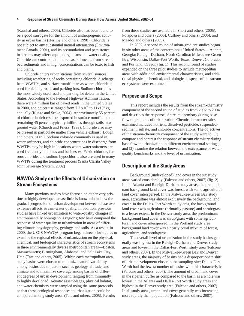
NAWQA Study on the Effects of Urbanization on Stream Ecosystems
Many previous studies have focused on either very pris-tine or highly developed areas; little is known about how the gradual progression of urban development between these two extremes affects stream-water quality. In addition, previous studies have linked urbanization to water-quality changes in environmentally homogenous regions; few have compared the response of water quality to urbanization in areas of differ-ing climate, physiography, geology, and soils. As a result, in 2000, the USGS NAWQA program began three pilot studies to examine the regional effects of urbanization on the physical, chemical, and biological characteristics of stream ecosystems in three environmentally diverse metropolitan areas—Boston, Massachusetts; Birmingham, Alabama; and Salt Lake City, Utah (Tate and others, 2005). Within each metropolitan area, study basins were chosen to minimize natural variability among basins due to factors such as geology, altitude, and climate and to maximize coverage among basins of differ-ent degrees of urban development, ranging from minimally to highly developed. Aquatic assemblages, physical habitat, and water chemistry were sampled using the same protocols so that these ecological responses to urbanization could be compared among study areas (Tate and others, 2005). Results
from these studies are available in Short and others (2005), Potapova and others (2005), Cuffney and others (2005), and Meador and others (2005).
In 2002, a second round of urban-gradient studies began in six other areas of the conterminous United States— Atlanta, Georgia; Raleigh-Durham, North Carolina; Milwaukee-Green Bay, Wisconsin; Dallas-Fort Worth, Texas; Denver, Colorado; and Portland, Oregon (fig. 1). This second round of studies expanded on the three pilot studies to include metropolitan areas with additional environmental characteristics, and addi-tional physical, chemical, and biological aspects of the stream ecosystems were examined.
Purpose and Scope
This report includes the results from the stream-chemistry component of the second round of studies from 2002 to 2004 and describes the response of stream chemistry during base flow to gradients of urbanization. Chemical characteristics examined included nutrient, dissolved pesticide, suspended-sediment, sulfate, and chloride concentrations. The objectives of the stream-chemistry component of the study were to: (1) compare and contrast the response of stream chemistry during base flow to urbanization in different environmental settings; and (2) examine the relation between the exceedance of water-quality benchmarks and the level of urbanization.
Description of the Study Areas
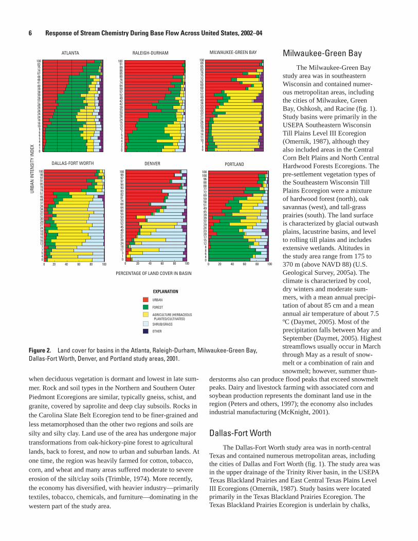
Background (undeveloped) land cover in the six study areas varied considerably (Falcone and others, 2007) (fig. 2). In the Atlanta and Raleigh-Durham study areas, the predomi-nant background land cover was forest, with some agricultural land cover interspersed. In the Milwaukee-Green Bay study area, agriculture was almost exclusively the background land cover. In the Dallas-Fort Worth study area, the background land cover was agriculture (primarily pasture) and shrub/grass to a lesser extent. In the Denver study area, the predominant background land cover was shrub/grass with some agricul-tural land cover interspersed. In the Portland study area, background land cover was a nearly equal mixture of forest, agriculture, and shrub/grass.
The overall level of urbanization in the study basins gen-erally was highest in the Raleigh-Durham and Denver study areas and lowest in the Dallas-Fort Worth study area (Falcone and others, 2007). In the Milwaukee-Green Bay and Denver study areas, the majority of basins had a disproportionate shift of urban development closer to the sampling site; Dallas-Fort Worth had the fewest number of basins with this characteristic (Falcone and others, 2007). The amount of urban land cover in the riparian buffer as compared to the basin as a whole was lowest in the Atlanta and Dallas-Fort Worth study areas and highest in the Denver study area (Falcone and others, 2007). In all study areas, urban land cover generally was increasing more rapidly than population (Falcone and others, 2007).
4 Response of Stream Chemistry During Base Flow Across United States, 2002–04

Salem
Dallas
Durham
Denver
Racine
Eugene
Atlanta
Boulder
Oshkosh
Marietta
Cheyenne
Portland
Green Bay
Corvallis
Fort Worth
EXPLANATION
Study area
City
WASHINGTON
WISCONSIN
NORTH CAROLINA
Denver
Portland
AtlantaGEORGIAALABAMA
TEXAS
COLORADO
WYOMING
OREGON
TEXAS State
Denver Study area name
Milwaukee-Green Bay
Raleigh-Durham
Winston-Salem Raleigh
Dallas-Fort Worth
Milwaukee
Fort Collins
Figure 1. Location of the study areas.
A general description of the six study areas follows (Fal-cone and others, 2007). These descriptions are based on the basins included in this study and may not be representative of the larger metropolitan areas.
Atlanta
The Atlanta study area was in north-central Georgia and portions of eastern Alabama and contained numerous met-ropolitan areas, including the cities of Atlanta and Marietta (fig. 1). Study basins were located entirely in the USEPA Piedmont Level III Ecoregion (Omernik, 1987), specifically in the Southern Inner and the Southern Outer Piedmont Level IV Ecoregions (U.S. Environmental Protection Agency, 2006a). The study area is characterized by gently rolling topography and dissected irregular plains, with altitudes ranging from about 100 to 465 m (above NAVD 88) (U.S. Geological Survey, 2005a). The climate is warm and humid, with a mean annual precipitation of about 131 cm and a mean annual air temperature of about 16.6 ºC (Daymet, 2005). Streams are typified by low to moderate gradients with cobble, gravel, and sandy substrates. Streamflow in the Southern Inner and Outer Piedmont Ecoregions generally is highest in the winter when rainfall primarily is derived from slow-moving frontal systems and lowest in late summer and fall when fast-moving thunderstorms are more prevalent. Potential natural vegeta-tion in the Southern Inner and Outer Piedmont Ecoregions is
oak–hickory–pine forest; however, current (2007) land use and land cover includes forested areas in silviculture as well as in agricultural production of hay, cattle, and poultry. The economy is well diversified, and although it includes industrial activities, it contains more commercial and service-oriented activity than heavy industry (McKnight, 2001).
Raleigh-Durham
The Raleigh-Durham study area was in north-central North Carolina and contained numerous metropolitan areas, including the cities of Raleigh, Durham, and Winston-Salem (fig. 1). Study basins were located entirely in the USEPA Piedmont Level III Ecoregion (Omernik, 1987), specifically in the Northern Outer Piedmont, Southern Outer Piedmont, and Carolina Slate Belt Level IV Ecoregions (U.S. Environmental Protection Agency, 2006a). The study area is characterized by irregular plains with some hills, with altitudes ranging from about 50 to 315 m (above NAVD 88) (U.S. Geological Survey, 2005a). The climate is warm and humid, with a mean annual precipitation of about 118 cm and a mean annual air tempera-ture of about 15.0 ºC (Daymet, 2005). Rainfall is evenly dis-tributed throughout the year, with slightly more rainfall in July and August and slightly less in October through December (Daymet, 2005). Streams in all three Level IV Ecoregions have low to moderate gradients and typically have gravel to cobble substrate. Streamflow typically is highest in the winter months
Introduction 5
when deciduous vegetation is dormant and lowest in late sum-mer. Rock and soil types in the Northern and Southern Outer Piedmont Ecoregions are similar, typically gneiss, schist, and granite, covered by saprolite and deep clay subsoils. Rocks in the Carolina Slate Belt Ecoregion tend to be finer-grained and less metamorphosed than the other two regions and soils are silty and silty clay. Land use of the area has undergone major transformations from oak-hickory-pine forest to agricultural lands, back to forest, and now to urban and suburban lands. At one time, the region was heavily farmed for cotton, tobacco, corn, and wheat and many areas suffered moderate to severe erosion of the silt/clay soils (Trimble, 1974). More recently, the economy has diversified, with heavier industry—primarily textiles, tobacco, chemicals, and furniture—dominating in the western part of the study area.
Milwaukee-Green BayThe Milwaukee-Green Bay
study area was in southeastern Wisconsin and contained numer-ous metropolitan areas, including the cities of Milwaukee, Green Bay, Oshkosh, and Racine (fig. 1). Study basins were primarily in the USEPA Southeastern Wisconsin Till Plains Level III Ecoregion (Omernik, 1987), although they also included areas in the Central Corn Belt Plains and North Central Hardwood Forests Ecoregions. The pre-settlement vegetation types of the Southeastern Wisconsin Till Plains Ecoregion were a mixture of hardwood forest (north), oak savannas (west), and tall-grass prairies (south). The land surface is characterized by glacial outwash plains, lacustrine basins, and level to rolling till plains and includes extensive wetlands. Altitudes in the study area range from 175 to 370 m (above NAVD 88) (U.S. Geological Survey, 2005a). The climate is characterized by cool, dry winters and moderate sum-mers, with a mean annual precipi-tation of about 85 cm and a mean annual air temperature of about 7.5 ºC (Daymet, 2005). Most of the precipitation falls between May and September (Daymet, 2005). Highest streamflows usually occur in March through May as a result of snow-melt or a combination of rain and snowmelt; however, summer thun-
derstorms also can produce flood peaks that exceed snowmelt peaks. Dairy and livestock farming with associated corn and soybean production represents the dominant land use in the region (Peters and others, 1997); the economy also includes industrial manufacturing (McKnight, 2001).
Dallas-Fort WorthThe Dallas-Fort Worth study area was in north-central
Texas and contained numerous metropolitan areas, including the cities of Dallas and Fort Worth (fig. 1). The study area was in the upper drainage of the Trinity River basin, in the USEPA Texas Blackland Prairies and East Central Texas Plains Level III Ecoregions (Omernik, 1987). Study basins were located primarily in the Texas Blackland Prairies Ecoregion. The Texas Blackland Prairies Ecoregion is underlain by chalks,
0 20 40 60 80 100 0 20 40 60 80 100
URBA
N IN
TEN
SITY
INDE
X
PERCENTAGE OF LAND COVER IN BASIN
DALLAS-FORT WORTH DENVER
0 20 40 60 80 100
PORTLAND
04577
1316161818242729303132343437444651747885919798
100
013
171824283737404552535354606468748182839394979799
100
04688
121517202324293239394549515859697277888896
100100
ATLANTA RALEIGH-DURHAM MILWAUKEE-GREEN BAY
01445669
101618242426262627283038394041464667747583
100
0224457
12131524282933394242495257596474768085868991
100
047
1011141919222627313333333840495253606062727576838589
100
EXPLANATION
URBAN
FOREST
AGRICULTURE (HERBACEOUS PLANTED/CULTIVATED)SHRUB/GRASS
OTHER
Figure 2. Land cover for basins in the Atlanta, Raleigh-Durham, Milwaukee-Green Bay, Dallas-Fort Worth, Denver, and Portland study areas, 2001.
6 Response of Stream Chemistry During Base Flow Across United States, 2002–04

marls, limestones, and shales and is a rolling to level plain with natural vegetation dominated by little bluestem, yel-low Indiangrass, sugar hackberry, bur oak, elm, and eastern cottonwood. Altitude in the study area ranges from about 80 to 270 m (above NAVD 88) (U.S. Geological Survey, 2005a). The climate is semiarid, with precipitation falling primarily in the spring and from summer thunderstorms. Mean annual precipitation is about 105 cm and mean annual air tempera-ture is about 18.2 ºC (Daymet, 2005). Streamflow in the study area is affected by reservoirs, intrabasin transfers, diversion of water for municipal water supply, and discharge from WWTPs. Smaller streams generally are intermittent. Land cover includes grassland, pasture, row crops, and urban areas. The economy includes finance, oil, transportation, aerospace, electronics, cattle, railways, and agriculture (McKnight, 2001).
Denver
The Denver study area was in north-central Colorado and southeastern Wyoming and contained numerous metropolitan areas, including the cities of Denver, Boulder, Fort Collins, and Cheyenne (fig. 1). Study basins were almost entirely in the USEPA Western High Plains Level III Ecoregion (Omernik, 1987), although one basin included a small area in the Southwestern Tablelands Ecoregion. Altitude in the study area ranges from about 1,465 to 2,545 m (above NAVD 88) (U.S. Geological Survey, 2005a); however, it is bordered by the Southern Rockies Ecoregion to the west, where altitudes are considerably higher. The climate is dry, with precipita-tion affected by topography. Most precipitation on the plains results from rainfall, primarily between April and September; however, during late spring and early summer, streamflow also is fed by snowmelt from the mountains, where snow falls dur-ing the winter. Mean annual precipitation is about 43 cm and mean annual air temperature is about 8.1 ºC (Daymet, 2005). A complex network of canals and pipes moves water between different areas for municipal water supply, agricultural irriga-tion, and power generation (Sprague and others, 2006). Land cover in the study area is dominated by grassland and agricul-ture in the plains, with conifer forest in the western mountains. The economy is diversified and includes agriculture, mining, and industry (McKnight, 2001).
Portland
The Portland study area was in western Oregon and parts of southern Washington and contained numerous metropolitan areas, including the cities of Portland, Salem, Corvallis, and Eugene (fig. 1). Study basins were primarily in the USEPA Willamette Valley Level III Ecoregion (Omernik, 1987), although they also included areas in the Coast Range and Cascades Ecoregions. The Willamette Valley Ecoregion is characterized as a broad, lowland valley with a mosaic of veg-etation of rolling prairies, deciduous and coniferous forests, and extensive wetlands. Landforms consist of terraces and
flood plains that are interlaced and surrounded by rolling hills. Altitude in the study area ranges from 0 to 1,330 m (above NAVD 88) (U.S. Geological Survey, 2005a) in the foothills of the Cascade Mountains. The climate is characterized by cool, wet winters and warm, dry summers with a mean annual precipitation of about 145 cm and a mean annual air tempera-ture of about 11.1 ºC (Daymet, 2005). Most of the precipita-tion falls between October and April. Highest streamflows are recorded from November to March and lowest streamflows occur in summer and fall. The economy includes forestry, fruit and wheat farming, dairying, and wood and food processing (McKnight, 2001).
Acknowledgments
The authors wish to thank all of those who conducted field work during this study and the many landowners and organizations that provided access to study sites. They also wish to acknowledge Barbara C. Ruddy and V. Cory Stephens with the U.S. Geological Survey for their assistance with data analysis.
ApproachWithin each study area, about 30 sites representing
minimal natural variability and a range of urbanization were selected. Water samples were collected twice at each site, once during low base-flow conditions and once during high base-flow conditions. Methods of site selection, sample collection, and data analysis are described as follows.
Geographic Information System Data
Using a Geographic Information System (GIS), about 300 urban and environmental variables were used to aid in site selection and data analysis (Falcone and others, 2007). Basin boundaries in most cases were derived from USGS 30-m resolution National Elevation Data (U.S. Geological Survey, 2005a) and in a small number of cases were refined from higher resolution data. Most variables were derived based on basin boundaries (basin-level variables); however, several categories of variables were calculated on finer scales (ripar-ian- and segment-level variables). Streams were based on the USGS National Hydrography Data 1:100,000 stream set (U.S. Geological Survey, 2005b). The GIS-derived variables fell into 11 broad categories:
(1) Population and housing: Counts of basin population and population density were calculated based on 2000 Census block-level data (GeoLytics, 2001). All other Census variables (demographic, labor, income, and housing characteristics) were calculated based on 2000 Census block-group data. In addition, four socioeconomic indices were derived based on principal component ordination of 63 Census variables, as
Approach 7

described in McMahon and Cuffney (2000). Each socioeco-nomic index represented a positive association with a subset of those variables and varied between study areas.
(2) Climate: Basin-level mean air temperature and pre-cipitation statistics were derived from 1-km resolution Daymet model data (Daymet, 2005), which represented temperature and precipitation averages over an 18-year period from 1980 to 1997. These data were obtained from terrain-adjusted daily climatological observations.
(3) Ecologic and hydrologic regions: Ecologic Region boundaries were based on USEPA level III Ecoregions for all study areas (Omernik, 1987). Additional level IV boundaries were used in the Raleigh-Durham, Milwaukee-Green Bay, and Dallas-Fort Worth study areas. Hydrologic Region boundaries were based on USGS Hydrologic Landscape Regions (Winter, 2001)).
(4) Infrastructure: Road data were based on Census 2000 Topologically Integrated Geographic Encoding and Reference line roads (GeoLytics, 2001). Point-source dischargers were derived from USEPA National Pollutant Discharge Elimina-tion System locations (U.S. Environmental Protection Agency, 2005f). Toxic release locations were derived from the USEPA Toxic Release Inventory (U.S. Environmental Protection Agency, 2005i). Dam location data were based on the U.S. Army Corps of Engineers National Inventory of Dams (U.S. Army Corps of Engineers, 1996).
(5) Land cover 2001, basin level: The 2001 land-cover data were based on the National Land Cover Data (NLCD) 2001 data set (for the Atlanta and Raleigh-Durham study areas) (U.S. Geological Survey, 2005c), National Oceanic and Atmospheric Administration (NOAA) Coastal Change Analysis Program (Portland study area) (National Oceanic and Atmospheric Administration, 2005), or derived using meth-ods and protocols identical to those used in the NLCD 2001 program (Milwaukee-Green Bay, Denver, and Dallas-Fort Worth study areas) (U.S. Geological Survey, 2006a). Likewise, NOAA land-cover data for the Portland study area were pro-duced using NLCD 2001 protocols, but these data contained slightly different class structures that were recoded to match the NLCD 2001 classes. The NLCD 2001 is a 30-m resolu-tion data set based primarily on Landsat-7 Enhanced Thematic Mapper imagery covering the period from 1999 to 2002. The NLCD 2001 program also contains a subpixel-percentage impervious-surface data layer, which was acquired or derived from imagery.
(6) Land cover 2001, riparian level: NLCD 2001 land-cover statistics were derived for riparian buffer based on the National Hydrography Data stream lines for the entire basin. The riparian buffer was defined as the area covering 100 m to each side of the stream centerline.
(7) Land cover 2001, distance weighted: Land cover in a number of basins was not spatially distributed evenly through-out the basin. Some basins had a small percentage of basin-level urban land use, but in the lower part of the basin near the sampling site, the percentage of urban land use was much higher. To address this finding, distance-weighted land-cover
data were calculated for each basin. The distance-weighted data were NLCD 2001 basin-level data re-weighted according to distance from the sampling site. Pixels representing land cover close to the sampling site were given a higher weight than those farther away; weights were calculated as the inverse distance from the sampling site. Distance-weighted land cover for each class then was calculated based on the distance-weighted data and normalized to 100 percent. The result was a percentage for each class that captured its spatial proximity to the sampling site.
(8) Land cover 2001, segment level: NLCD 2001 land-cover statistics were derived for the riparian zone (100 m on each side of stream centerline) of the segment of stream just upstream from the sampling location. The distance upstream was a function of the basin area. Segment statistics also were calculated for non-land cover physical characteristics—sinu-osity, gradient, mean distance to nearest road, and density of road and stream intersections on the length of the segment.
(9) Land cover 1992, basin level: The 1992 land-cover data were based on the NLCD 1992 data set.
(10) Landscape pattern: Landscape-pattern metrics char-acterizing the shape, size, and spatial configuration of land-cover patches were derived using the FRAGSTATS software package (McGarigal and others, 2002). FRAGSTATS metrics were calculated for patches of each land-cover class. An addi-tional metric (basin-shape index) was calculated based on the entire basin boundary.
(11) Soils and topography: Soil properties were derived from the U.S. Department of Agriculture State Soil Geo-graphic data base (U.S. Department of Agriculture, 1994). Topographic characteristics were derived from USGS 30-m resolution National Elevation Data (U.S. Geological Survey, 2005a).
Site Selection
About 30 sites within each study area were selected on the basis of two major factors: (1) variability in natural land-scape features and (2) gradient in the degree of urbanization.
Variability in Natural Landscape FeaturesWithin each study area, sites were selected to minimize
natural variability between basins to reduce the potential for natural factors to confound the interpretation of the chemical response along the urban land-use gradient (Falcone and oth-ers, 2007). GIS-derived data were used to identify candidate basins in each area with similar environmental characteris-tics. Basin boundaries were delineated based on USGS 30-m National Elevation Data (U.S. Geological Survey, 2005a). The major initial filtering criteria for natural landscape features were ecoregion, soils, and topography. USEPA Ecoregions (Omernik, 1987) provided a coarse framework of relatively homogenous climate, altitude, soils, geology, and vegetation (Tate and others, 2005). Most candidate basins for each study
8 Response of Stream Chemistry During Base Flow Across United States, 2002–04

area fell within a single USEPA level III Ecoregion. Cluster analysis (Everitt and others, 2001) of climate, altitude, slope, soils, vegetation, and geology variables then was performed to group the candidate basins on the basis of environmental char-acteristics. From the resulting clusters, a final set of candidate basins was identified with similar natural landscape features. Each study area had a different number of final candidate basins (Atlanta–217; Raleigh-Durham–1,245; Milwaukee-Green Bay–51; Dallas-Fort Worth–57; Denver–162; Portland–171), but all were selected with the same goal of minimizing natural variability.
Gradient in the Degree of UrbanizationRather than studying a single site over a long period
as it urbanized, the goal of this study was to look at a larger number of sites that ranged from minimally to highly devel-oped over a short time. In theory, the pattern of the chemical response among environmentally homogenous sites spanning a range of urbanization in space could reflect the same pattern of response that would be seen as a minimally disturbed site urbanized over time. Therefore, the second consideration for site selection was the need to obtain study sites that covered a gradient of urbanization from minimally to highly developed.
Previous studies of urban ecosystems have suggested that land use alone is not an adequate measure of urbaniza-tion (McMahon and Cuffney, 2000; Grove and Burch, 1997). In this study, land cover, infrastructure, and socioeconomic variables were integrated in a multimetric urban intensity index (UII) that was used to represent overall urbanization. A UII value was calculated for each of the basins by using a five-step procedure described in McMahon and Cuffney (2000). In brief, the procedure consisted of the following: (1) adjust-ing urban variables for basin size and measurement units, (2) range standardizing the original variables so the values ranged from 0 to 100, (3) retaining variables correlated with popula-tion density and uncorrelated with basin area and adjusting the variables so they all increased with increasing population den-sity, (4) averaging retained variables across each site to obtain a UII, and (5) range standardizing the UII at each site so the values collectively ranged from 0 to 100. The criteria used in determining whether variables were correlated with popula-tion density varied among study areas; details are provided in Falcone and others (2007). The final variables included in the UII for each metropolitan area also are provided in Falcone and others (2007).
Once the candidate sites were identified through cluster analysis and the UII values were calculated for each, field reconnaissance took place to ground-truth the GIS data and to evaluate logistical issues, such as site access and safety condi-tions. Some sites were relocated short distances up or down-stream to provide better access, to obtain reaches with cobble or riffle substrate, or to minimize local effects from wastewa-ter-treatment-plant effluent, major diversions, or upstream res-ervoir releases. Some sites automatically were excluded based upon evidence that the stream was ephemeral. Other sites were
excluded if access permissions could not be obtained from landowners. Ultimately, about 30 sites were selected in each study area; these sites were selected to be as evenly distributed as possible between minimally and highly developed condi-tions. The desired number of sites was set at about 30 for each study area because when a sample size is greater than 25–30, the sampling distribution of the mean becomes approximately normal (Hogg and Tanis, 1993). The final list of sites in each study area is provided in Falcone and others (2007).
Data Collection
Environmental Samples
Environmental water-chemistry samples were collected from October 2002 through September 2004. Samples were collected twice at each site, once during low base-flow condi-tions and once during high base-flow conditions (table 1). In addition, 10 out of the approximately 30 sites included in each study area were sampled bimonthly for 1 year to document potential seasonal variability in the response of base-flow chemistry to urbanization that may have been missed by sam-pling only twice at the majority of sites. The results from the samples collected during high and low base-flow conditions are the focus of this report; the results from the bimonthly
Table 1. Dates of sample collection during high and low base-flow conditions for each of the six study areas.
Study area
High base-flowsample
Low base-flowsample
Atlanta, Georgia March 2003 September 2003
Raleigh-Durham, North Carolina
February 2003 July 2003
Milwaukee-Green Bay, Wisconsin
May – June 2004
August 2004
Dallas-Fort Worth, Texas May 2004 February 2004Denver, Colorado June 2003 August 2003
Portland, Oregon May 2004 August 2004
sampling to evaluate seasonal variability are presented and discussed briefly in Appendix 1. For this report, the low base-flow period was defined as a period in which, under average climatic conditions, there are few precipitation events; the high base-flow period was defined as a period in which, under average climatic conditions, there are more frequent precipi-tation events and streamflow is derived to a greater degree from recent rain and(or) snowfall. The low and high base-flow periods were determined based on seasonal variability in streamflow and climate, as summarized in the “Description of the Study Areas” section.
In the Raleigh-Durham, Milwaukee-Green Bay, and Dallas-Fort Worth study areas, a slightly different set of sites was sampled during low base-flow conditions than during high
Approach 9

base-flow conditions because some sites went dry between the two sampling periods and some sites that were sampled once were later deemed inappropriate for subsequent sampling of aquatic communities (Falcone and others, 2007). In some instances, a dropped site was replaced with another site with similar urban characteristics; in other instances, no replace-ment was made. Although water-chemistry conditions can vary substantially between base-flow and storm-runoff condi-tions because of differing transport mechanisms and instream dilution capacities, the scope of this study was not large enough to fully characterize chemical conditions during base flow and stormflow runoff.
All sites were sampled for nutrients, dissolved pesticides and pesticide degradates, suspended sediment, sulfate, and chloride in water (table 2). In addition, field measurements were obtained for water temperature, dissolved oxygen, pH, specific conductance, and discharge at the time of sampling. Water samples were collected using standardized depth- and width-integrating techniques and were processed and preserved onsite using standard methods described in U.S. Geological Survey (variously dated). Samples were filtered prior to analysis of dissolved constituents, including pesticides (0.7-µm pore diameter) and some nutrients (0.45-µm pore diameter), to remove suspended particulate matter. Nutrient and pesticide samples were analyzed at the USGS National Water-Quality Laboratory in Denver, Colo., by using methods described in Fishman (1993) and Zaugg and others (1995), respectively. Suspended-sediment samples were analyzed at USGS Water Science Center Sediment Laboratories in Louisi-ana, Iowa, and Kentucky, and at the USGS Cascades Volcano Observatory in Washington (Guy, 1969). Water-chemistry data are available in the USGS National Water Information System, accessible at http://waterdata.usgs.gov/nwis/qw.
Quality-Control SamplesQuality-control samples, including field blanks, repli-
cates, and laboratory spikes, were collected throughout the study. Quality-control data are presented in Appendix 2. Over-all, 57 field blanks were collected to identify the presence and magnitude of any contamination, 23 replicates were collected to evaluate variability due to sample collection and process-ing and laboratory analysis, and 21 field spikes were collected to evaluate bias in the recovery of pesticides. More detail on quality-control design and sampling for surface-water studies in the NAWQA program is available in Mueller and others (1997).
Data Analysis
Data CompilationWhenever possible, chemical samples were collected
during base-flow conditions. Some samples, however, were
collected during unavoidable or unanticipated elevated streamflow conditions caused by snowmelt, reservoir releases, or localized storm runoff. Examination of the hydrographs at each site indicates that less than about 15 percent of the samples were collected during elevated streamflow conditions; these samples were collected at sites covering a wide range of UII values. Such samples will increase the nonurban-related variability in the data. However, these were not high-leverage or influential points, and they were retained in the data set to maintain coverage over the urban gradient.
Total nitrogen was calculated for each sample by sum-ming either: (1) total Kjeldahl nitrogen and dissolved nitrite-plus-nitrate or (2) dissolved ammonia, dissolved nitrite-plus-nitrate, and particulate nitrogen. If all addends were censored, total nitrogen was censored to the maximum of the censoring levels; if one was uncensored and the others were censored, total nitrogen was set equal to the uncensored value; if two were uncensored and the other was censored, total nitrogen was set equal to the sum of the uncensored values. Total herbicide and total insecticide concentrations were calculated for each sample as the sum of their respective components. Censored values were set to zero and estimated values were used without modification during these calculations.
A pesticide toxicity index (PTI) value, which takes into account the presence of multiple pesticides in a sample (Munn and Gilliom, 2001), also was calculated for each sample. The PTI combines information on exposure of aquatic biota to pes-ticides (measured concentrations of pesticides in stream water) with toxicity estimates (results from laboratory toxicity stud-ies) to produce a relative index value for a sample or stream. The PTI value was computed for each sample of stream water by summing the toxicity quotients for all pesticides detected in the sample. The toxicity quotient was the measured concentra-tion of a pesticide in a stream sample divided by its median toxicity concentration from bioassays (such as a 50-percent lethal concentration [LC50
] or a 50-percent effect concentration [EC
50]). Separate PTI values were computed for fish and cla-
docerans (commonly referred to as water fleas). In this report, PTI values were computed using median toxicity concentra-tions obtained from Munn and others (2006).
The PTI has several important limitations. First, the PTI approach assumes that toxicity is additive and combines toxic-ity-weighted concentrations of pesticides from multiple chemi-cal classes without regard to mode of action. This approach, likewise, does not account for synergistic or antagonistic effects. Moreover, toxicity values are based on bioassays of acute exposure and do not include effects of chronic exposure. Environmental factors that can affect bioavailability and toxic-ity (such as dissolved organic carbon and temperature) are not accounted for in the PTI. The PTI is limited to pesticides measured in the water column; hydrophobic pesticides may be underrepresented in potential toxicity (especially to benthic organisms). Because toxicity values from different sources vary, there is considerable uncertainty in the relative toxicity of pesticides with only a few bioassays available (the number of bioassays varied among pesticides from 1 to 165 for a given
10 Response of Stream Chemistry During Base Flow Across United States, 2002–04

ConstituentUSGS
parameter code
Chemical class
Pesticide use
Parent compound
Ammonia plus organic (Kjeldahl) nitrogen, water, unfiltered (mg/L as N) 00625 na na na
Nitrite plus nitrate, water, filtered (mg/L as N) 00631 na na na
Ammonia, water, filtered (mg/L as N) 00608 na na na
Particulate nitrogen, suspended in water (mg/L as N) 49570 na na na
Nitrate, water, filtered (mg/L as N) 00618 na na na
Phosphorus, water, unfiltered (mg/L as P) 00665 na na na
Orthophosphate, water, filtered (mg/L as P) 00671 na na na
1-Naphthol, water, filtered, recoverable (µg/L) 49295 Phenol Degradate Carbaryl, napropamide
2,6-Diethylaniline, water, filtered, recoverable (µg/L) 82660 Degradate Degradate Alachlor
2-[(2-Ethyl-6-methylphenyl)-amino]-1-propanol, water, filtered, recoverable (µg/L) 61615 Aniline Degradate Metolachlor
2-Chloro-2’,6’-diethylacetanilide, water, filtered, recoverable (µg/L) 61618 Acetanilide Degradate Alachlor
2-Chloro-4-isopropylamino-6-amino-s-triazine, water, filtered, recoverable (µg/L) 04040 Triazine Degradate Atrazine
2-Ethyl-6-methylaniline, water, filtered, recoverable (µg/L) 61620 Aniline Degradate Metolachlor
3,4-Dichloroaniline, water, filtered, recoverable (µg/L) 61625 Aniline Degradate Diuron/propanil/linuron/neburon
4-Chloro-2-methylphenol, water, filtered, recoverable (µg/L) 61633 Phenol Degradate MCPA/MCPB
Acetochlor, water, filtered, recoverable (µg/L) 49260 Acetanilide Herbicide na
Alachlor, water, filtered, recoverable (µg/L) 46342 Acetanilide Herbicide na
Atrazine, water, filtered, recoverable (µg/L) 39632 Triazine Herbicide na
Azinphos-methyl oxygen analog, water, filtered, recoverable (µg/L) 61635 Organophosphate Degradate Azinphos-methyl
Azinphos-methyl, water, filtered, recoverable (µg/L) 82686 Organophosphate Insecticide na
Benfluralin, water, filtered, recoverable (µg/L) 82673 Dinitroaniline Herbicide na
Carbaryl, water, filtered, recoverable (µg/L) 82680 Carbamate Insecticide na
Chlorpyrifos oxygen analog, water, filtered, recoverable (µg/L) 61636 Organophosphate Degradate Chlorpyrifos
Chlorpyrifos, water, filtered, recoverable (µg/L) 38933 Organophosphate Insecticide na
cis-Permethrin, water, filtered, recoverable (µg/L) 82687 Pyrethroid Insecticide na
Cyfluthrin, water, filtered, recoverable (µg/L) 61585 Pyrethroid Insecticide na
Cypermethrin, water, filtered, recoverable (µg/L) 61586 Pyrethroid Insecticide na
Dacthal (DCPA), water, filtered, recoverable (µg/L) 82682 Chlorobenzoic acid ester Herbicide na
Desulfinyl fipronil, water, filtered, recoverable (µg/L) 62170 Phenyl pyrazole Degradate Fipronil
Diazinon oxygen analog, water, filtered, recoverable (µg/L) 61638 Organophosphate Degradate Diazinon
Table 2. Chemical constituents analyzed in base-flow samples.
[USGS, U.S. Geological Survey; na, not applicable; mg/L, milligrams per liter; N, nitrogen; P, phosphorus; mg/L, micrograms per liter; MCPA, (4-chloro-2-methyphenoxy) acetic acid; MCPB, Thistol]
Approach
11
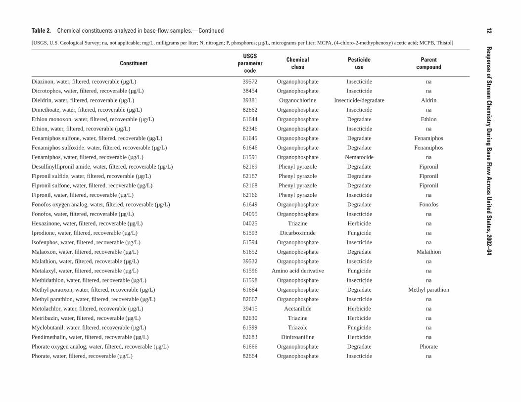
ConstituentUSGS
parameter code
Chemical class
Pesticide use
Parent compound
Diazinon, water, filtered, recoverable (µg/L) 39572 Organophosphate Insecticide na
Dicrotophos, water, filtered, recoverable (µg/L) 38454 Organophosphate Insecticide na
Dieldrin, water, filtered, recoverable (µg/L) 39381 Organochlorine Insecticide/degradate Aldrin
Dimethoate, water, filtered, recoverable (µg/L) 82662 Organophosphate Insecticide na
Ethion monoxon, water, filtered, recoverable (µg/L) 61644 Organophosphate Degradate Ethion
Ethion, water, filtered, recoverable (µg/L) 82346 Organophosphate Insecticide na
Fenamiphos sulfone, water, filtered, recoverable (µg/L) 61645 Organophosphate Degradate Fenamiphos
Fenamiphos sulfoxide, water, filtered, recoverable (µg/L) 61646 Organophosphate Degradate Fenamiphos
Fenamiphos, water, filtered, recoverable (µg/L) 61591 Organophosphate Nematocide na
Desulfinylfipronil amide, water, filtered, recoverable (µg/L) 62169 Phenyl pyrazole Degradate Fipronil
Fipronil sulfide, water, filtered, recoverable (µg/L) 62167 Phenyl pyrazole Degradate Fipronil
Fipronil sulfone, water, filtered, recoverable (µg/L) 62168 Phenyl pyrazole Degradate Fipronil
Fipronil, water, filtered, recoverable (µg/L) 62166 Phenyl pyrazole Insecticide na
Fonofos oxygen analog, water, filtered, recoverable (µg/L) 61649 Organophosphate Degradate Fonofos
Fonofos, water, filtered, recoverable (µg/L) 04095 Organophosphate Insecticide na
Hexazinone, water, filtered, recoverable (µg/L) 04025 Triazine Herbicide na
Iprodione, water, filtered, recoverable (µg/L) 61593 Dicarboximide Fungicide na
Isofenphos, water, filtered, recoverable (µg/L) 61594 Organophosphate Insecticide na
Malaoxon, water, filtered, recoverable (µg/L) 61652 Organophosphate Degradate Malathion
Malathion, water, filtered, recoverable (µg/L) 39532 Organophosphate Insecticide na
Metalaxyl, water, filtered, recoverable (µg/L) 61596 Amino acid derivative Fungicide na
Methidathion, water, filtered, recoverable (µg/L) 61598 Organophosphate Insecticide na
Methyl paraoxon, water, filtered, recoverable (µg/L) 61664 Organophosphate Degradate Methyl parathion
Methyl parathion, water, filtered, recoverable (µg/L) 82667 Organophosphate Insecticide na
Metolachlor, water, filtered, recoverable (µg/L) 39415 Acetanilide Herbicide na
Metribuzin, water, filtered, recoverable (µg/L) 82630 Triazine Herbicide na
Myclobutanil, water, filtered, recoverable (µg/L) 61599 Triazole Fungicide na
Pendimethalin, water, filtered, recoverable (µg/L) 82683 Dinitroaniline Herbicide na
Phorate oxygen analog, water, filtered, recoverable (µg/L) 61666 Organophosphate Degradate Phorate
Phorate, water, filtered, recoverable (µg/L) 82664 Organophosphate Insecticide na
Table 2. Chemical constituents analyzed in base-flow samples.—Continued
[USGS, U.S. Geological Survey; na, not applicable; mg/L, milligrams per liter; N, nitrogen; P, phosphorus; mg/L, micrograms per liter; MCPA, (4-chloro-2-methyphenoxy) acetic acid; MCPB, Thistol]
12
Response of Stream Chem
istry During Base Flow Across United States, 2002–04

ConstituentUSGS
parameter code
Chemical class
Pesticide use
Parent compound
Phosmet oxygen analog, water, filtered, recoverable (µg/L) 61668 Organophosphate Degradate Phosmet
Phosmet, water, filtered, recoverable (µg/L) 61601 Organophosphate Insecticide na
Prometon, water, filtered, recoverable (µg/L) 04037 Triazine Herbicide na
Prometryn, water, filtered, recoverable (µg/L) 04036 Triazine Herbicide na
Pronamide, water, filtered, recoverable (µg/L) 82676 Amide Herbicide na
Simazine, water, filtered, recoverable (µg/L) 04035 Triazine Herbicide na
Tebuthiuron, water, filtered, recoverable (µg/L) 82670 Urea Herbicide na
Terbufos oxygen analog sulfone, water, filtered, recoverable (µg/L) 61674 Organophosphate Degradate Terbufos
Terbufos, water, filtered, recoverable (µg/L) 82675 Organophosphate Insecticide na
Terbuthylazine, water, filtered, recoverable (µg/L) 04022 Triazine Herbicide na
Trifluralin, water, filtered, recoverable (µg/L) 82661 Dinitroaniline Herbicide na
Dichlorvos, water, filtered, recoverable (µg/L) 38775 OrganophosphateInsecticide, fumigant,
degradateNaled
pH, water, unfiltered (standard units) 00400 na na na
Suspended sediment concentration (mg/L) 80154 na na na
Sulfate, water, filtered (mg/L) 00945 na na na
Chloride, water, filtered (mg/L) 00940 na na na
Table 2. Chemical constituents analyzed in base-flow samples.—Continued
[USGS, U.S. Geological Survey; na, not applicable; mg/L, milligrams per liter; N, nitrogen; P, phosphorus; mg/L, micrograms per liter; MCPA, (4-chloro-2-methyphenoxy) acetic acid; MCPB, Thistol]
Approach
13

taxonomic group). Finally, not all important local species were included in bioassays. Despite its limitations, the PTI approach can be a useful tool for examining pesticide mixtures in streams—such as in investigating relations between concentra-tions of multiple pesticides detected in a stream and the quality of aquatic ecosystems. It also provides a mechanism for con-sidering the potential contribution to toxicity of pesticides that do not have established benchmarks for aquatic life. The PTI does not indicate whether water in a sample or stream is toxic; however, its value can be used to rank or compare the relative potential toxicity of different samples or different streams.
Quality-Control AnalysisQuality-control samples, including blanks, replicates,
and laboratory spikes, were evaluated prior to data analysis (Appendix 2). Concentrations in the blanks generally were below the laboratory reporting levels; two blanks from the Raleigh-Durham study area had total ammonia plus organic (Kjeldahl) nitrogen concentrations greater than the reporting level. Because the main focus of the data analysis in this report is comparing responses among sites (as opposed to looking at chemical characteristics at a single site), this isolated, low-level contamination likely did not substantially influence the results.
The mean relative percent difference (relative percent difference =|A-B|/[(A+B)/2], where A is the environmental sample concentration and B is the replicate sample concentra-tion) between the paired replicate samples was greater than 10 percent for particulate nitrogen, total phosphorus, 2-chloro-4-isopropylamino-6-amino-s-triazine, 3,4-dichloroaniline, 4-chloro-2-methylphenol, desulfinyl fipronil, diazinon, dieldrin, prometon, tebuthiuron, and suspended sediment, indicting that for these constituents, the variability in concentration due to field and laboratory procedures may have been greater than the variability in concentration between some sites. Concentra-tions of other constituents were consistent between the paired replicate samples; mean relative percent differences were less than 10 percent.
Phosmet and phosmet oxygen analog had false negatives (no detections in spike) in nine pesticide spikes from multiple study areas, likely indicating a systemic problem in the labora-tory. As a result, phosmet and phosmet oxygen analog were treated as missing in all environmental samples. Two con-stituents (2-[(2-ethyl-6-methylphenyl)-amino]-1-propanol and iprodione) had false negatives from sites in the Atlanta study area, indicating that something at those sites may have caused incorrect quantitation; these constituents were treated as miss-ing in all environmental samples from the affected sites only.
When a given constituent shows a false negative in a spike, there is a chance that true, detectable concentrations are being reported as censored in environmental samples. In environmental samples with reported detections, the constitu-ent is most likely present but the reported concentration may be biased low. When a false negative occurs, treating detect-able environmental concentrations as missing results in a loss
of information. However, because the main focus of the data analysis is comparing responses among sites (as opposed to looking at chemical characteristics at a single site), the pos-sibility of false negatives in censored environmental samples would introduce too much uncertainty.
Mean spike recoveries of less than 50 percent were found for 1-naphthol, 2-chloro-4-isopropylamino-6-amino-s-triazine, dicrotophos, dimethoate, iprodione, phosmet oxygen analog, and phosmet. Recoveries consistently were low among all spikes for phosmet and phosmet oxygen analog, dimethoate, dicrotophos, and 2-chloro-4-isopropylamino-6-amino-s-tri-azine; low but consistent recoveries are suitable for the data analysis in this study. Recoveries were much more variable for 1-naphthol (mean of 27 percent, standard deviation of 22 percent) and iprodione (mean of 32 percent, standard deviation of 24 percent); this degree of variability was not acceptable for the data analysis in this study. As a result, 1-naphthol and ipro-dione were treated as missing in all environmental samples.
Patterns of Response to Urbanization Correlation analysis was used to assess the strength of the
relation between each chemical constituent and the percent-age of urban land cover in the basin. Because of the potential for nonlinear relations, Spearman’s rho, which is based on the ranks of the values and thus can account for monotonic curvi-linearity, was used as the measure of correlation. Spearman’s rho is dimensionless and scaled to range from -1 to 1 (Helsel and Hirsch, 1992). When there was no correlation between the concentration of a chemical and the percentage of urban land cover in the basin, Spearman’s rho equaled 0; when the chemi-cal concentration increased as the percentage of urban land cover in the basin increased, Spearman’s rho was positive; when they varied in opposite directions, Spearman’s rho was negative. In this application, the results of significance tests may be inaccurate because single test p-values can underesti-mate the probability of error when many dependent correla-tions (that is, comparisons to the same variable) are tested (Van Sickle, 2003). In addition, the sample size within each study area was small relative to the variance, resulting in low power to detect real correlations; rejecting the null hypotheses (x and y are not correlated) would likely be far less common than not rejecting the null hypothesis (Parkhurst, 2001). As a result, the focus in this report is on the strength of the rela-tions instead of the apparent significance of the relations. Relative classifications of the strength of the relations were based on the range of correlation values in the data for the six study areas. Typically, relations were described as “strong” if the absolute value of Spearman’s rho was approximately 0.5 or greater, although the use of an absolute threshold value to characterize “strong” relations (for example, in which a cor-relation coefficient of 0.50 was “strong” and 0.49 was “weak”) was rejected as arbitrary.
A scatterplot with a locally weighted scatterplot smooth (LOWESS) also was made to examine the pattern of the rela-tion between each chemical constituent and the percentage of
14 Response of Stream Chemistry During Base Flow Across United States, 2002–04

urban land cover in the basin (urban land cover as used here is the aggregated NLCD 2001 level 1 “developed” category, including developed open space and low-, medium-, and high-intensity development). Comparisons were made among study areas to examine the response of water chemistry to urbaniza-tion in different environmental settings.
The strengths of these relations also were compared during high and low base-flow conditions within each study area to examine the influence of hydrologic variability on the response of water chemistry to urbanization. When the sites sampled during high and low base-flow conditions differed (Raleigh-Durham, Milwaukee-Green Bay, and Dallas Fort-Worth), Fisher’s test for nonoverlapping correlations (Fisher, 1921) was used to test whether the correlations between the percentage of urban land cover in the basin and chemical concentrations at high base flow were significantly different from the correlation between the percentage of urban land cover in the basin and chemical concentrations at low base flow. When the sites sampled during high and low base-flow conditions were the same (Atlanta, Denver, and Portland), the method described in Meng and others (1992) for overlapping correlations was used. The strengths of the relations during high and low base-flow conditions were considered signifi-cantly different if the p-value for Fisher’s or Meng’s test was less than or equal to 0.05. These tests likely were subject to the same low-power limitation as was the Spearman’s rank correlation analysis; therefore, the null hypothesis of Fisher’s and Meng’s test (correlations during high and low base-flow conditions were not different) may have been rejected less fre-quently than would have occurred if more data were available. In some instances, the relation between two variables was “strong” (absolute value of Spearman’s rho was approximately 0.5 or greater) during one base-flow condition and “weak” (absolute value of Spearman’s rho was less than approximately 0.5) during the other base-flow condition, but the results from the Fisher’s or Meng’s test indicated there was no statistically significant difference. In these instances, no distinction could be made between the strength of these relations during inter-pretation—lacking evidence to the contrary, if one relation was strong, both were considered to be strong.
Because the multimetric UII values were range standard-ized using values at just the sites within each study area, and because a different set of urban variables was used to calculate the UII in each study area, these local UII values were not directly comparable across study areas. To create a common basis for comparing sites across all study areas, a common UII was developed by using the same urban variables to calculate the UII at all sites in all study areas and then range standard-izing across all of these sites (Falcone and others, 2007). However, local differences led to difficulties in identifying consistent, representative urban gradients in individual study areas and in creating common UII values that corresponded to the local UII values used during site selection (Falcone and others, 2007). As a result, neither the local UII values nor the common UII values were used in the data analysis for this report. Instead, the response of water chemistry to urbaniza-
tion was examined by using the percentage of urban land cover in the basin as a surrogate for “urbanization.” The percentage of urban land cover in the basin does not reflect simultaneous urban influences as the UII does, but because it was con-sistently derived in all study areas, it is directly comparable across environmental settings. With this approach, differences among environmental settings in the relation between water chemistry and urbanization can be attributed to regional differ-ences in the gradient of urban land cover without the potential confounding influence of regional differences in the calcula-tion of the UII. Spearman’s rank correlations between the local UII and the percentage of urban land cover in the basin were high (0.98 in Atlanta, 0.98 in Raleigh-Durham, 0.98 in Mil-waukee-Green Bay, 0.87 in Dallas-Fort Worth, 0.96 in Denver, and 0.97 in Portland); therefore, any differences in interpreta-tion should be minimal in all study areas.
Spearman’s rank correlation analysis also was used to assess the strength of the association between each chemical variable and additional urban and landscape variables. The goal of this analysis was to determine which urban variables were most strongly associated with the chemical variables and to identify any nonurban landscape variables that may have been confounding the response to urbanization. Of the approx-imately 300 urban and landscape variables produced to aid in site selection and data analysis, 22 are highlighted in this report (table 3). (See Sprague and others (2006) for a full list of urban and landscape variables produced to aid in site selec-tion and data analysis). These 22 variables were selected from among groups of related variables (for example, road density was chosen from among road length, road-area index, road-traffic index, road-area density, road-traffic density, and road density; the percentage of forested land cover in the basin was strongly related to the percentage of urban land cover in the basin, so only the percentage of urban land cover in the basin was highlighted) or in lieu of a group of categorical variables that each contained a large number of zeros (for example, a variable representing the sand content of the soil was chosen in lieu of individual soil texture classification and hydrologic soil groups). As with the percentage of urban land cover in the basin, Fisher’s test for nonoverlapping correlations and the method described in Meng and others (1992) for overlapping correlations were used to test whether the correlations between these additional urban and landscape features and chemical concentrations were significantly different during high base-flow and low base-flow conditions.
There is an important limitation in the interpretation of the relations between chemical concentrations and landscape variables in this study. In the hypothetical case of a strong relation between total nitrogen concentrations and the land-scape variable basin slope in the Denver study area, basin slope would not necessarily be strongly related to total nitro-gen concentrations in the greater (unsampled) Denver-Fort Collins-Cheyenne area. The 28 sites in the Denver study area were chosen to cover an urban gradient with the intent of mini-mizing variability in natural landscape features, such as basin slope. As a result, the range of basin slope covered by the
Approach 15
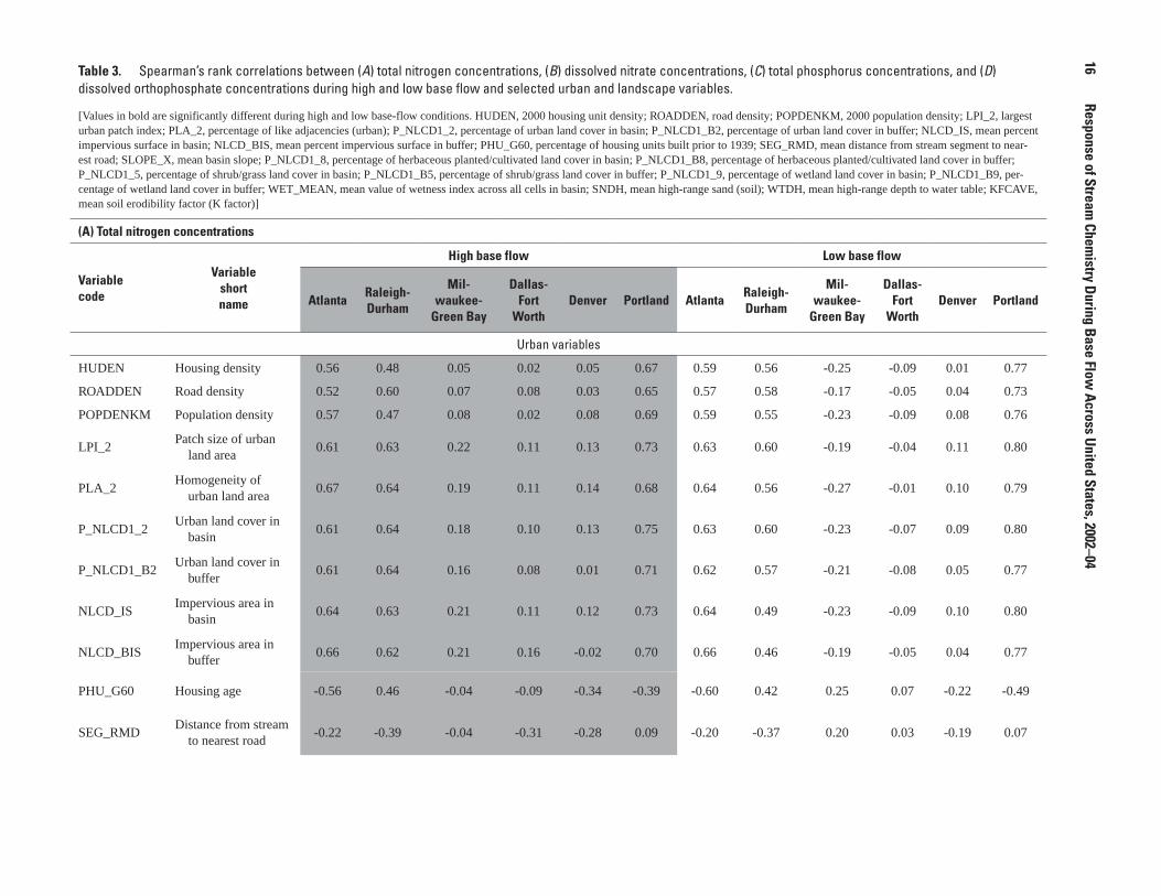
Table 3. Spearman’s rank correlations between (A) total nitrogen concentrations, (B) dissolved nitrate concentrations, (C) total phosphorus concentrations, and (D) dissolved orthophosphate concentrations during high and low base flow and selected urban and landscape variables.
[Values in bold are significantly different during high and low base-flow conditions. HUDEN, 2000 housing unit density; ROADDEN, road density; POPDENKM, 2000 population density; LPI_2, largest urban patch index; PLA_2, percentage of like adjacencies (urban); P_NLCD1_2, percentage of urban land cover in basin; P_NLCD1_B2, percentage of urban land cover in buffer; NLCD_IS, mean percent impervious surface in basin; NLCD_BIS, mean percent impervious surface in buffer; PHU_G60, percentage of housing units built prior to 1939; SEG_RMD, mean distance from stream segment to near-est road; SLOPE_X, mean basin slope; P_NLCD1_8, percentage of herbaceous planted/cultivated land cover in basin; P_NLCD1_B8, percentage of herbaceous planted/cultivated land cover in buffer; P_NLCD1_5, percentage of shrub/grass land cover in basin; P_NLCD1_B5, percentage of shrub/grass land cover in buffer; P_NLCD1_9, percentage of wetland land cover in basin; P_NLCD1_B9, per-centage of wetland land cover in buffer; WET_MEAN, mean value of wetness index across all cells in basin; SNDH, mean high-range sand (soil); WTDH, mean high-range depth to water table; KFCAVE, mean soil erodibility factor (K factor)]
(A) Total nitrogen concentrations
Variable code
Variable short name
High base flow Low base flow
AtlantaRaleigh-Durham
Mil -waukee-
Green Bay
Dallas-Fort
WorthDenver Portland Atlanta
Raleigh-Durham
Mil -waukee-
Green Bay
Dallas-Fort
WorthDenver Portland
Urban variables
HUDEN Housing density 0.56 0.48 0.05 0.02 0.05 0.67 0.59 0.56 -0.25 -0.09 0.01 0.77
ROADDEN Road density 0.52 0.60 0.07 0.08 0.03 0.65 0.57 0.58 -0.17 -0.05 0.04 0.73
POPDENKM Population density 0.57 0.47 0.08 0.02 0.08 0.69 0.59 0.55 -0.23 -0.09 0.08 0.76
LPI_2Patch size of urban
land area0.61 0.63 0.22 0.11 0.13 0.73 0.63 0.60 -0.19 -0.04 0.11 0.80
PLA_2Homogeneity of
urban land area0.67 0.64 0.19 0.11 0.14 0.68 0.64 0.56 -0.27 -0.01 0.10 0.79
P_NLCD1_2Urban land cover in
basin0.61 0.64 0.18 0.10 0.13 0.75 0.63 0.60 -0.23 -0.07 0.09 0.80
P_NLCD1_B2Urban land cover in
buffer0.61 0.64 0.16 0.08 0.01 0.71 0.62 0.57 -0.21 -0.08 0.05 0.77
NLCD_ISImpervious area in
basin0.64 0.63 0.21 0.11 0.12 0.73 0.64 0.49 -0.23 -0.09 0.10 0.80
NLCD_BISImpervious area in
buffer0.66 0.62 0.21 0.16 -0.02 0.70 0.66 0.46 -0.19 -0.05 0.04 0.77
PHU_G60 Housing age -0.56 0.46 -0.04 -0.09 -0.34 -0.39 -0.60 0.42 0.25 0.07 -0.22 -0.49
SEG_RMDDistance from stream
to nearest road-0.22 -0.39 -0.04 -0.31 -0.28 0.09 -0.20 -0.37 0.20 0.03 -0.19 0.07
16
Response of Stream Chem
istry During Base Flow Across United States, 2002–04

Table 3. Spearman’s rank correlations between (A) total nitrogen concentrations, (B) dissolved nitrate concentrations, (C) total phosphorus concentrations, and (D) dissolved orthophosphate concentrations during high and low base flow and selected urban and landscape variables.
[Values in bold are significantly different during high and low base-flow conditions. HUDEN, 2000 housing unit density; ROADDEN, road density; POPDENKM, 2000 population density; LPI_2, largest urban patch index; PLA_2, percentage of like adjacencies (urban); P_NLCD1_2, percentage of urban land cover in basin; P_NLCD1_B2, percentage of urban land cover in buffer; NLCD_IS, mean percent impervious surface in basin; NLCD_BIS, mean percent impervious surface in buffer; PHU_G60, percentage of housing units built prior to 1939; SEG_RMD, mean distance from stream segment to near-est road; SLOPE_X, mean basin slope; P_NLCD1_8, percentage of herbaceous planted/cultivated land cover in basin; P_NLCD1_B8, percentage of herbaceous planted/cultivated land cover in buffer; P_NLCD1_5, percentage of shrub/grass land cover in basin; P_NLCD1_B5, percentage of shrub/grass land cover in buffer; P_NLCD1_9, percentage of wetland land cover in basin; P_NLCD1_B9, per-centage of wetland land cover in buffer; WET_MEAN, mean value of wetness index across all cells in basin; SNDH, mean high-range sand (soil); WTDH, mean high-range depth to water table; KFCAVE, mean soil erodibility factor (K factor)]
(A) Total nitrogen concentrations
Variable code
Variable short name
High base flow Low base flow
AtlantaRaleigh-Durham
Mil -waukee-
Green Bay
Dallas-Fort
WorthDenver Portland Atlanta
Raleigh-Durham
Mil -waukee-
Green Bay
Dallas-Fort
WorthDenver Portland
Lanscape variables
SLOPE_X Basin slope 0.01 -0.40 -0.04 0.10 -0.24 -0.80 -0.10 -0.44 0.15 -0.11 -0.34 -0.79
P_NLCD1_8Agricultural land
cover in basin-0.20 -0.46 0.03 0.01 -0.12 0.21 -0.12 -0.48 -0.03 0.38 0.15 0.14
P_NLCD1_B8Agricultural land
cover in buffer-0.10 -0.43 0.18 0.05 -0.09 0.17 -0.09 -0.42 -0.01 0.37 0.09 0.14
P_NLCD1_5Shrub/grass land
cover in basin-0.62 -0.57 0.02 -0.18 -0.06 -0.73 -0.65 -0.47 -0.11 -0.02 -0.13 -0.78
P_NLCD1_B5Shrub/grass land
cover in buffer-0.52 -0.55 0.03 -0.22 0.09 -0.68 -0.58 -0.43 -0.18 0.07 0.00 -0.77
P_NLCD1_9Wetland land cover in
basin-0.10 -0.44 -0.31 0.18 0.14 0.08 0.00 -0.51 0.25 0.26 0.07 -0.07
P_NLCD1_B9Wetland land cover in
buffer-0.12 -0.47 -0.26 0.25 0.14 -0.06 0.00 -0.47 0.23 0.36 0.08 -0.14
WET_MEAN Basin-wetness index -0.05 0.18 -0.04 -0.04 0.02 0.74 0.05 0.19 -0.15 0.07 0.33 0.70
SNDH Sand content in soil -0.11 -0.17 -0.41 0.33 -0.04 -0.28 0.18 0.10 0.33 0.36 -0.06 -0.33
WTDH Depth to water table 0.44 0.18 -0.34 -0.15 -0.03 -0.36 0.42 0.29 0.08 -0.32 -0.02 -0.41
KFCAVE Soil erodibility 0.31 -0.47 0.22 0.05 0.27 0.39 0.29 -0.58 -0.09 0.13 0.56 0.39
Approach
17

Table 3. Spearman’s rank correlations between (A) total nitrogen concentrations, (B) dissolved nitrate concentrations, (C) total phosphorus concentrations, and (D) dissolved orthophosphate concentrations during high and low base flow and selected urban and landscape variables.—Continued
[Values in bold are significantly different during high and low base-flow conditions. HUDEN, 2000 housing unit density; ROADDEN, road density; POPDENKM, 2000 population density; LPI_2, largest urban patch index; PLA_2, percentage of like adjacencies (urban); P_NLCD1_2, percentage of urban land cover in basin; P_NLCD1_B2, percentage of urban land cover in buffer; NLCD_IS, mean percent impervious surface in basin; NLCD_BIS, mean percent impervious surface in buffer; PHU_G60, percentage of housing units built prior to 1939; SEG_RMD, mean distance from stream segment to near-est road; SLOPE_X, mean basin slope; P_NLCD1_8, percentage of herbaceous planted/cultivated land cover in basin; P_NLCD1_B8, percentage of herbaceous planted/cultivated land cover in buffer; P_NLCD1_5, percentage of shrub/grass land cover in basin; P_NLCD1_B5, percentage of shrub/grass land cover in buffer; P_NLCD1_9, percentage of wetland land cover in basin; P_NLCD1_B9, percent-age of wetland land cover in buffer; WET_MEAN, mean value of wetness index across all cells in basin; SNDH, mean high-range sand (soil); WTDH, mean high-range depth to water table; KFCAVE, mean soil erodibility factor (K factor)]
(B) Dissolved nitrate concentrations
Variable code
Variable short name
High base flow Low base flow
AtlantaRaleigh-Durham
Mil-waukee-
Green Bay
Dallas-Fort
WorthDenver Portland Atlanta
Raleigh-Durham
Mil-waukee-
Green Bay
Dallas-Fort
WorthDenver Portland
Urban variables
HUDEN Housing density 0.55 0.42 0.08 0.10 0.11 0.60 0.58 0.33 -0.27 -0.08 0.03 0.70
ROADDEN Road density 0.55 0.52 0.10 0.16 0.05 0.59 0.57 0.41 -0.19 -0.05 0.07 0.68
POPDENKM Population density 0.58 0.40 0.11 0.08 0.14 0.63 0.59 0.32 -0.25 -0.10 0.10 0.69
LPI_2Patch size of urban
land area0.59 0.54 0.27 0.16 0.14 0.67 0.64 0.43 -0.21 -0.06 0.13 0.73
PLA_2Homogeneity of
urban land area0.63 0.51 0.24 0.15 0.16 0.60 0.63 0.40 -0.29 -0.03 0.09 0.72
P_NLCD1_2Urban land cover in
basin0.59 0.55 0.21 0.15 0.13 0.68 0.63 0.43 -0.25 -0.08 0.11 0.74
P_NLCD1_B2Urban land cover in
buffer0.59 0.55 0.20 0.17 0.01 0.65 0.63 0.43 -0.23 -0.08 0.06 0.70
NLCD_ISImpervious area in
basin0.61 0.49 0.25 0.16 0.12 0.67 0.64 0.36 -0.25 -0.11 0.12 0.75
NLCD_BISImpervious area in
buffer0.64 0.48 0.27 0.23 -0.02 0.63 0.68 0.36 -0.22 -0.07 0.04 0.70
PHU_G60 Housing age -0.60 0.59 -0.01 -0.15 -0.32 -0.31 -0.66 0.56 0.25 0.05 -0.30 -0.40
SEG_RMDDistance from
stream to nearest road
-0.16 -0.47 -0.08 -0.37 -0.34 0.14 -0.16 -0.49 0.22 0.02 -0.13 0.15
18
Response of Stream Chem
istry During Base Flow Across United States, 2002–04

Table 3. Spearman’s rank correlations between (A) total nitrogen concentrations, (B) dissolved nitrate concentrations, (C) total phosphorus concentrations, and (D) dissolved orthophosphate concentrations during high and low base flow and selected urban and landscape variables.—Continued
[Values in bold are significantly different during high and low base-flow conditions. HUDEN, 2000 housing unit density; ROADDEN, road density; POPDENKM, 2000 population density; LPI_2, largest urban patch index; PLA_2, percentage of like adjacencies (urban); P_NLCD1_2, percentage of urban land cover in basin; P_NLCD1_B2, percentage of urban land cover in buffer; NLCD_IS, mean percent impervious surface in basin; NLCD_BIS, mean percent impervious surface in buffer; PHU_G60, percentage of housing units built prior to 1939; SEG_RMD, mean distance from stream segment to near-est road; SLOPE_X, mean basin slope; P_NLCD1_8, percentage of herbaceous planted/cultivated land cover in basin; P_NLCD1_B8, percentage of herbaceous planted/cultivated land cover in buffer; P_NLCD1_5, percentage of shrub/grass land cover in basin; P_NLCD1_B5, percentage of shrub/grass land cover in buffer; P_NLCD1_9, percentage of wetland land cover in basin; P_NLCD1_B9, percent-age of wetland land cover in buffer; WET_MEAN, mean value of wetness index across all cells in basin; SNDH, mean high-range sand (soil); WTDH, mean high-range depth to water table; KFCAVE, mean soil erodibility factor (K factor)]
(B) Dissolved nitrate concentrations
Variable code
Variable short name
High base flow Low base flow
AtlantaRaleigh-Durham
Mil-waukee-
Green Bay
Dallas-Fort
WorthDenver Portland Atlanta
Raleigh-Durham
Mil-waukee-
Green Bay
Dallas-Fort
WorthDenver Portland
Landscape variablesSLOPE_X Basin slope 0.25 -0.40 -0.10 0.22 -0.24 -0.75 -0.02 -0.42 0.20 -0.07 -0.48 -0.72
P_NLCD1_8Agricultural land
cover in basin-0.11 -0.43 0.02 -0.03 -0.09 0.17 -0.11 -0.33 -0.03 0.38 0.23 0.05
P_NLCD1_B8Agricultural land
cover in buffer0.10 -0.43 0.17 0.00 -0.08 0.11 -0.01 -0.32 -0.02 0.36 0.16 0.04
P_NLCD1_5Shrub/grass land
cover in basin-0.59 -0.52 0.01 -0.19 -0.02 -0.67 -0.66 -0.36 -0.10 -0.03 -0.13 -0.70
P_NLCD1_B5Shrub/grass land
cover in buffer-0.51 -0.55 0.04 -0.27 0.13 -0.60 -0.60 -0.42 -0.17 0.05 -0.06 -0.68
P_NLCD1_9Wetland land cover
in basin-0.23 -0.53 -0.36 0.16 0.11 0.09 -0.04 -0.56 0.27 0.25 0.00 -0.09
P_NLCD1_B9Wetland land cover
in buffer-0.20 -0.52 -0.33 0.23 0.11 -0.06 -0.02 -0.63 0.26 0.34 0.02 -0.16
WET_MEAN Basin-wetness index -0.21 0.19 0.00 -0.11 0.07 0.68 -0.09 0.23 -0.20 0.05 0.48 0.62
SNDH Sand content in soil -0.03 -0.09 -0.50 0.31 -0.04 -0.22 0.04 0.05 0.34 0.29 -0.12 -0.27
WTDH Depth to water table 0.31 0.19 -0.35 -0.12 -0.08 -0.30 0.39 0.23 0.15 -0.27 -0.02 -0.37
KFCAVE Soil erodibility 0.22 -0.47 0.30 0.03 0.29 0.34 0.33 -0.46 -0.09 0.09 0.70 0.30
Approach
19

Table 3. Spearman’s rank correlations between (A) total nitrogen concentrations, (B) dissolved nitrate concentrations, (C) total phosphorus concentrations, and (D) dissolved orthophosphate concentrations during high and low base flow and selected urban and landscape variables.—Continued
[Values in bold are significantly different during high and low base-flow conditions. HUDEN, 2000 housing unit density; ROADDEN, road density; POPDENKM, 2000 population density; LPI_2, larg-est urban patch index; PLA_2, percentage of like adjacencies (urban); P_NLCD1_2, percentage of urban land cover in basin; P_NLCD1_B2, percentage of urban land cover in buffer; NLCD_IS, mean percent impervious surface in basin; NLCD_BIS, mean percent impervious surface in buffer; PHU_G60, percentage of housing units built prior to 1939; SEG_RMD, mean distance from stream segment to nearest road; SLOPE_X, mean basin slope; P_NLCD1_8, percentage of herbaceous planted/cultivated land cover in basin; P_NLCD1_B8, percentage of herbaceous planted/cultivated land cover in buffer; P_NLCD1_5, percentage of shrub/grass land cover in basin; P_NLCD1_B5, percentage of shrub/grass land cover in buffer; P_NLCD1_9, percentage of wetland land cover in basin; P_NLCD1_B9, percentage of wetland land cover in buffer; WET_MEAN, mean value of wetness index across all cells in basin; SNDH, mean high-range sand (soil); WTDH, mean high-range depth to water table; KFCAVE, mean soil erodibility factor (K factor)]
(C) Total phosphorus concentrations
Variable code
Variableshort name
High base flow Low base flow
AtlantaRaleigh-Durham
Mil-waukee-
Green Bay
Dallas-Fort
Worth Denver Portland Atlanta
Raleigh-Durham
Mil-waukee-
Green Bay
Dallas-Fort
Worth Denver Portland
Urban variables
HUDEN Housing density 0.08 0.01 -0.61 -0.06 0.26 0.65 0.23 0.17 -0.22 0.22 0.34 0.76
ROADDEN Road density 0.00 0.01 -0.63 -0.13 0.31 0.61 0.16 0.19 -0.28 0.17 0.30 0.65
POPDENKM Population density 0.01 0.02 -0.62 -0.08 0.26 0.67 0.15 0.20 -0.20 0.21 0.35 0.76
LPI_2Patch size of urban
land area0.08 0.03 -0.61 -0.08 0.38 0.65 0.22 0.10 -0.13 0.25 0.36 0.75
PLA_2Homogeneity of
urban land area0.13 0.04 -0.61 -0.07 0.40 0.66 0.28 0.12 -0.15 0.27 0.41 0.76
P_NLCD1_2Urban land cover in
basin0.07 0.05 -0.58 -0.06 0.38 0.64 0.22 0.14 -0.16 0.25 0.35 0.71
P_NLCD1_B2Urban land cover in
buffer0.07 0.00 -0.64 -0.15 0.33 0.60 0.19 0.10 -0.23 0.10 0.34 0.69
NLCD_ISImpervious area in
basin0.06 0.08 -0.56 -0.08 0.39 0.65 0.22 0.16 -0.12 0.25 0.37 0.73
NLCD_BISImpervious area in
buffer0.06 0.10 -0.61 -0.11 0.34 0.61 0.21 0.11 -0.10 0.14 0.35 0.69
PHU_G60 Housing age 0.01 -0.21 0.44 0.05 -0.32 -0.30 -0.10 -0.06 0.21 -0.15 -0.19 -0.42
SEG_RMDDistance from
stream to nearest road
0.07 0.12 0.56 0.01 -0.33 -0.11 -0.11 0.21 0.14 -0.11 -0.33 -0.05
Landscape variables
SLOPE_X Basin slope -0.69 -0.09 -0.19 -0.35 -0.29 -0.53 -0.37 0.09 -0.47 -0.21 0.11 -0.61
P_NLCD1_8Agricultural land
cover in basin0.02 0.13 0.66 0.15 -0.21 0.04 -0.08 -0.04 0.34 -0.02 -0.36 0.11
P_NLCD1_B8Agricultural land
cover in buffer-0.12 0.22 0.67 0.23 -0.18 0.02 -0.17 0.03 0.43 0.02 -0.32 0.03
20
Response of Stream Chem
istry During Base Flow Across United States, 2002–04

Table 3. Spearman’s rank correlations between (A) total nitrogen concentrations, (B) dissolved nitrate concentrations, (C) total phosphorus concentrations, and (D) dissolved orthophosphate concentrations during high and low base flow and selected urban and landscape variables.—Continued
[Values in bold are significantly different during high and low base-flow conditions. HUDEN, 2000 housing unit density; ROADDEN, road density; POPDENKM, 2000 population density; LPI_2, larg-est urban patch index; PLA_2, percentage of like adjacencies (urban); P_NLCD1_2, percentage of urban land cover in basin; P_NLCD1_B2, percentage of urban land cover in buffer; NLCD_IS, mean percent impervious surface in basin; NLCD_BIS, mean percent impervious surface in buffer; PHU_G60, percentage of housing units built prior to 1939; SEG_RMD, mean distance from stream segment to nearest road; SLOPE_X, mean basin slope; P_NLCD1_8, percentage of herbaceous planted/cultivated land cover in basin; P_NLCD1_B8, percentage of herbaceous planted/cultivated land cover in buffer; P_NLCD1_5, percentage of shrub/grass land cover in basin; P_NLCD1_B5, percentage of shrub/grass land cover in buffer; P_NLCD1_9, percentage of wetland land cover in basin; P_NLCD1_B9, percentage of wetland land cover in buffer; WET_MEAN, mean value of wetness index across all cells in basin; SNDH, mean high-range sand (soil); WTDH, mean high-range depth to water table; KFCAVE, mean soil erodibility factor (K factor)]
(C) Total phosphorus concentrations
Variable code
Variableshort name
High base flow Low base flow
AtlantaRaleigh-Durham
Mil-waukee-
Green Bay
Dallas-Fort
Worth Denver Portland AtlantaRaleigh-Durham
Mil-waukee-
Green Bay
Dallas-Fort
Worth Denver Portland
Landscape variables
P_NLCD1_5Shrub/grass land
cover in basin-0.18 -0.07 -0.35 -0.09 -0.14 -0.56 -0.16 -0.20 -0.23 -0.37 -0.07 -0.66
P_NLCD1_B5Shrub/grass land
cover in buffer-0.11 0.02 -0.56 0.02 -0.17 -0.59 -0.10 -0.11 -0.33 -0.19 -0.05 -0.69
P_NLCD1_9Wetland land cover
in basin 0.47 0.16 0.33 0.07 0.19 0.16 0.37 0.02 -0.15 0.31 0.15 0.05
P_NLCD1_B9Wetland land cover
in buffer 0.39 0.03 0.27 0.06 0.23 0.11 0.29 0.11 -0.22 0.41 0.13 -0.02
WET_MEAN Basin-wetness index 0.54 0.15 0.17 0.34 0.35 0.47 0.40 -0.07 0.49 0.26 -0.04 0.52
SNDH Sand content in soil 0.10 -0.11 0.22 0.07 -0.18 -0.67 0.23 0.09 -0.11 0.19 -0.24 -0.77WTDH Depth to water table 0.42 -0.08 0.24 -0.26 -0.12 -0.77 0.36 0.11 0.18 -0.24 -0.22 -0.77KFCAVE Soil erodibility 0.42 0.03 -0.33 0.36 0.47 0.63 0.28 -0.16 -0.10 0.34 0.15 0.73
Approach
21

Table 3. Spearman’s rank correlations between (A) total nitrogen concentrations, (B) dissolved nitrate concentrations, (C) total phosphorus concentrations, and (D) dissolved orthophosphate concentrations during high and low base flow and selected urban and landscape variables.—Continued
[Values in bold are significantly different during high and low base-flow conditions. HUDEN, 2000 housing unit density; ROADDEN, road density; POPDENKM, 2000 population density; LPI_2, largest urban patch index; PLA_2, percentage of like adjacencies (urban); P_NLCD1_2, percentage of urban land cover in basin; P_NLCD1_B2, percentage of urban land cover in buffer; NLCD_IS, mean percent impervious surface in basin; NLCD_BIS, mean percent impervious surface in buffer; PHU_G60, percentage of housing units built prior to 1939; SEG_RMD, mean distance from stream segment to near-est road; SLOPE_X, mean basin slope; P_NLCD1_8, percentage of herbaceous planted/cultivated land cover in basin; P_NLCD1_B8, percentage of herbaceous planted/cultivated land cover in buffer; P_NLCD1_5, percentage of shrub/grass land cover in basin; P_NLCD1_B5, percentage of shrub/grass land cover in buffer; P_NLCD1_9, percentage of wetland land cover in basin; P_NLCD1_B9, percent-age of wetland land cover in buffer; WET_MEAN, mean value of wetness index across all cells in basin; SNDH, mean high-range sand (soil); WTDH, mean high-range depth to water table; KFCAVE, mean soil erodibility factor (K factor)]
(D) Dissolved orthophosphate concentrations
Variable code
Variable short name
High base flow Low base flow
Atlanta Raleigh-Durham
Mil-waukee-
Green Bay
Dallas-Fort
WorthDenver Portland Atlanta
Raleigh-Durham
Mil-wakee-
Green Bay
Dallas-Fort
WorthDenver Portland
Urban variablesHUDEN Housing density 0.16 -0.33 -0.53 0.05 -0.01 0.58 -0.34 -0.12 -0.33 0.08 0.22 0.60
ROADDEN Road density 0.18 -0.30 -0.56 -0.05 -0.03 0.47 -0.35 -0.03 -0.35 0.03 0.19 0.50
POPDENKM Population density 0.15 -0.32 -0.55 0.01 0.02 0.57 -0.34 -0.13 -0.30 0.04 0.23 0.60
LPI_2Patch size of urban land area
0.18 -0.30 -0.48 -0.06 -0.05 0.58 -0.23 -0.05 -0.25 0.07 0.26 0.61
PLA_2Homogeneity of
urban land area0.17 -0.28 -0.49 -0.08 0.04 0.59 -0.20 -0.04 -0.28 0.11 0.33 0.61
P_NLCD1_2Urban land cover
in basin0.17 -0.29 -0.48 -0.01 -0.05 0.55 -0.24 -0.03 -0.29 0.09 0.25 0.58
P_NLCD1_B2Urban land cover
in buffer0.18 -0.31 -0.53 0.01 -0.08 0.52 -0.25 -0.05 -0.33 -0.02 0.24 0.53
NLCD_ISImpervious area in
basin0.12 -0.23 -0.45 -0.07 -0.03 0.57 -0.27 0.06 -0.24 0.06 0.29 0.60
NLCD_BISImpervious area in
buffer0.12 -0.27 -0.48 0.04 -0.06 0.52 -0.25 0.06 -0.22 0.02 0.25 0.54
PHU_G60 Housing age 0.08 -0.26 0.53 -0.10 0.35 -0.30 0.25 0.31 0.34 -0.13 -0.11 -0.29
SEG_RMDDistance from
stream to near-est road
-0.30 0.04 0.48 -0.18 -0.07 0.14 0.36 0.14 0.22 -0.03 -0.19 0.15
Landscape variablesSLOPE_X Basin slope -0.23 -0.14 -0.31 -0.13 -0.21 -0.49 -0.28 -0.16 -0.35 0.08 0.01 -0.54
P_NLCD1_8Agricultural land
cover in basin-0.24 0.26 0.66 -0.06 0.11 -0.14 -0.09 0.16 0.42 -0.01 -0.21 -0.02
P_NLCD1_B8Agricultural land
cover in buffer-0.29 0.26 0.71 -0.01 0.13 -0.18 -0.14 0.31 0.49 0.00 -0.20 -0.07
22
Response of Stream Chem
istry During Base Flow Across United States, 2002–04
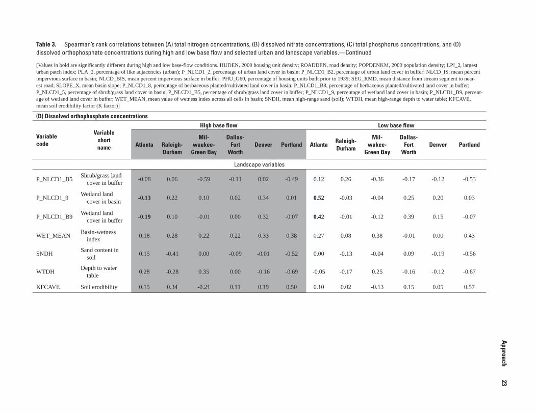
Table 3. Spearman’s rank correlations between (A) total nitrogen concentrations, (B) dissolved nitrate concentrations, (C) total phosphorus concentrations, and (D) dissolved orthophosphate concentrations during high and low base flow and selected urban and landscape variables.—Continued
[Values in bold are significantly different during high and low base-flow conditions. HUDEN, 2000 housing unit density; ROADDEN, road density; POPDENKM, 2000 population density; LPI_2, largest urban patch index; PLA_2, percentage of like adjacencies (urban); P_NLCD1_2, percentage of urban land cover in basin; P_NLCD1_B2, percentage of urban land cover in buffer; NLCD_IS, mean percent impervious surface in basin; NLCD_BIS, mean percent impervious surface in buffer; PHU_G60, percentage of housing units built prior to 1939; SEG_RMD, mean distance from stream segment to near-est road; SLOPE_X, mean basin slope; P_NLCD1_8, percentage of herbaceous planted/cultivated land cover in basin; P_NLCD1_B8, percentage of herbaceous planted/cultivated land cover in buffer; P_NLCD1_5, percentage of shrub/grass land cover in basin; P_NLCD1_B5, percentage of shrub/grass land cover in buffer; P_NLCD1_9, percentage of wetland land cover in basin; P_NLCD1_B9, percent-age of wetland land cover in buffer; WET_MEAN, mean value of wetness index across all cells in basin; SNDH, mean high-range sand (soil); WTDH, mean high-range depth to water table; KFCAVE, mean soil erodibility factor (K factor)]
(D) Dissolved orthophosphate concentrations
Variable code
Variable short name
High base flow Low base flow
Atlanta Raleigh-Durham
Mil-waukee-
Green Bay
Dallas-Fort
WorthDenver Portland Atlanta
Raleigh-Durham
Mil-wakee-
Green Bay
Dallas-Fort
WorthDenver Portland
Landscape variables
P_NLCD1_B5Shrub/grass land
cover in buffer-0.08 0.06 -0.59 -0.11 0.02 -0.49 0.12 0.26 -0.36 -0.17 -0.12 -0.53
P_NLCD1_9Wetland land
cover in basin-0.13 0.22 0.10 0.02 0.34 0.01 0.52 -0.03 -0.04 0.25 0.20 0.03
P_NLCD1_B9Wetland land
cover in buffer-0.19 0.10 -0.01 0.00 0.32 -0.07 0.42 -0.01 -0.12 0.39 0.15 -0.07
WET_MEANBasin-wetness
index0.18 0.28 0.22 0.22 0.33 0.38 0.27 0.08 0.38 -0.01 0.00 0.43
SNDHSand content in
soil0.15 -0.41 0.00 -0.09 -0.01 -0.52 0.00 -0.13 -0.04 0.09 -0.19 -0.56
WTDHDepth to water
table0.28 -0.28 0.35 0.00 -0.16 -0.69 -0.05 -0.17 0.25 -0.16 -0.12 -0.67
KFCAVE Soil erodibility 0.15 0.34 -0.21 0.11 0.19 0.50 0.10 0.02 -0.13 0.15 0.05 0.57
Approach
23

study basins may not be representative of the range in basin slope encountered in the greater Denver-Fort Collins-Chey-enne area. If that full range in basin slope had been covered by the study basins, the strength of the relation between total nitrogen concentrations and basin slope might have been sig-nificantly different (as likely also would be the strength of the relation between total nitrogen concentrations and urbaniza-tion). The relations with landscape variables were determined in this study to identify potential confounding influences along the urban gradient and to examine how those influences varied among environmental settings.
The analyses described previously were repeated for each chemical constituent under 12 scenarios. Each of the six study areas was examined independently, with the high base-flow and low base-flow data examined separately.
Benchmark ExceedancesChemical concentrations were compared to water-quality
benchmarks in a screening-level assessment of the potential importance of nutrients, pesticides, pH, sulfate, and chloride to human health and aquatic life in each study area. The screen-ing-level assessment is not a substitute for risk assessment, which includes many more factors, such as additional avenues of exposure. The screening-level results are intended primarily to identify areas for further investigation and as a tool to assess the relative potential for effects in relation to urbanization in different environmental settings.
Human-Health and Drinking-Water Benchmarks
Four types of human-health benchmarks were used to assess the potential for nutrients and pesticides in base flow to affect human health. Of the constituents that were sampled, one or more human-health benchmarks currently (2007) are available for four nutrients (Appendix 3), 36 of the 41 pesti-cides, and none of the 24 pesticide degradates (Appendix 4) measured in this study. Technically, these benchmarks apply to finished drinking water consumed over a lifetime, whereas this study measured nutrients and pesticides in relatively few samples of stream water over a year; for the most part, these stream sites were not near drinking-water intakes. Therefore, these human-health benchmarks were not used to evaluate actual human exposure to contaminants or to ascertain viola-tion of any drinking-water standards, but rather as general reference levels for putting measured concentrations in a human-health context.
In addition to the four types of human-health benchmarks for nutrients and pesticides, pH and concentrations of sulfate and chloride were compared with USEPA secondary drink-ing-water regulations (SDWRs), which pertain to the cosmetic and aesthetic effects of drinking water (Appendix 3). As with the human-health benchmarks for nutrients and pesticides, SDWRs apply to finished drinking water; as a result, the SDWRs have been used as general benchmarks or reference levels in this report.
The four types of human-health benchmarks and relevant SDWRs used in this study are as follows:
USEPA Maximum Contaminant Level (MCL)• —The maximum permissible concentration of a contaminant in water that is delivered to any user of a public-water system. This is an enforceable standard issued by USEPA under the Safe Drinking Water Act and is established on the basis of health effects and other factors (analytical and treatment technologies, and cost). As noted above, MCLs are used in this report as general benchmarks; the sampling design of this study does not meet the sampling and analytical conditions required to ascertain violation of drinking-water stan-dards. MCLs are available for three nutrients and three pesticides (U.S. Environmental Protection Agency, 2006b) analyzed for this study (Appendixes 3 and 4).
USEPA Lifetime Health Advisory (LHA)• —The concentration of a chemical in drinking water that is not expected to cause any adverse, noncarcinogenic effects over a lifetime exposure. A health advisory is a human-health guideline (issued in advisory capacity), not a legally enforceable Federal standard. It assumes lifetime consumption of 2 L of water per day by a 70-kg adult, and that 20 percent of total exposure to the contaminant comes from drinking water (80 percent is assumed to come from other sources). LHA values are available for 1 nutrient and for 14 unregulated pesti-cides (that is, pesticides without MCLs) (U.S. Envi-ronmental Protection Agency, 2006b) analyzed for this study (Appendixes 3 and 4).
USEPA 10• -6 Cancer Risk Concentration (10-6 CRC)—The concentration of a chemical in drinking water corresponding to an excess estimated lifetime cancer risk of 1 in a million (10-6). These human-health guidelines are calculated from the estimated cancer potency, which is derived using a conservative (protec-tive) model of carcinogenesis, so that the cancer risk is an upper-limit estimate. The definition of “acceptable” level of cancer risk is a policy issue, not a scientific one. USEPA reviews individual State and Tribal poli-cies on cancer risk levels as part of its oversight of water-quality standards under the Clean Water Act. USEPA’s policy is to accept measures adopted by States to limit cancer risk to the range of 10-6 to 10-4 (U.S. Environmental Protection Agency, 1992). The concentration corresponding to a cancer risk of 10-6 was used as the benchmark for the screening-level assessment in this study, consistent with the protective nature of such assessments. Values of 10-6 CRC are available for four unregulated pesticides (U.S. Environ-mental Protection Agency, 2005d, 2006b) analyzed for this study (Appendix 4).
USGS Health-Based Screening Level (HBSL)• —An estimate of concentration (for a noncarcinogen)
24 Response of Stream Chemistry During Base Flow Across United States, 2002–04
or concentration range (for a carcinogen) in water that may be of potential human-health concern, if exceeded. HBSLs are nonenforceable benchmarks that were developed by the USGS in collaboration with USEPA and others using USEPA methodologies for establishing drinking-water guidelines and the most current, USEPA peer-reviewed, publicly available human-health toxicity information (Toccalino and oth-ers, 2003, 2006). HBSLs were derived for unregulated pesticides only (those without USEPA MCLs) and on the basis of health effects only, to assist with evaluation of concentrations of unregulated pesticides in water-quality assessments. Note that, for contaminants that are likely or potential carcinogens, the HBSL assumes a specific cancer risk. Consistent with the 10-6 CRC values, in this study HBSL values for carcinogens assumed a 10-6 cancer risk. HBSLs are available for 33 pesticides (many of which also have LHA or 10-6 CRC values), but not for any nutrients (U.S. Geological Sur-vey, 2006b) analyzed for this study (Appendix 4).
USEPA Secondary Drinking-Water Regulations •(SDWR)—Nonenforceable Federal guidelines regard-ing cosmetic effects (such as tooth or skin discolor-ation) or aesthetic effects (such as taste, odor, or color) of drinking water. SDWRs are drinking-water bench-marks, but not human-health benchmarks. They are available for pH, chloride, and sulfate (U.S. Environ-mental Protection Agency, 2006b) (Appendix 3).
Human-health benchmarks were selected for each constituent as follows—if available, the MCL was used as the human-health benchmark. For constituents with no MCL, comparisons were made with all applicable guidelines (LHA, 10-6 CRC, and(or) HBSL). For this report, human-health and SDWR benchmarks were compared to constituent concentra-tions in individual samples because too few samples were collected to compute annual mean concentrations.
Aquatic-Life Benchmarks
Benchmarks for assessing the potential for nutrients, pesticides, pH, and chloride in base flow to adversely affect aquatic life fall into two groups: (1) USEPA ambient water-quality criteria for the protection of aquatic life (AWQC-AL), which were developed by the USEPA Office of Water and are available for selected nutrients, pesticides, pH, and chloride; and (2) additional pesticide benchmarks derived from toxicity values in pesticide registration and risk-assessment documents prepared by the USEPA Office of Pesticide Programs. One or more aquatic-life benchmarks are available for one nutrient, pH, chloride, (Appendix 3), and 37 of the 65 pesticides and degradates (Appendix 4) measured in this study.
Ambient Water-Quality Criteria for Aquatic Organisms
The USEPA Office of Water derives aquatic-life criteria for priority pollutants and other selected contaminants under
acute and chronic exposure conditions. Each acute and chronic criterion specifies a threshold concentration for unacceptable potential for effects, an averaging period, and an acceptable frequency of exceedance. AWQC-ALs are available for one nutrient, pH, chloride, 4 of the 41 pesticides, and none of the 24 pesticide degradates measured for this study (Appendixes 3 and 4). For ammonia, numeric criteria values were calcu-lated for each water sample because the criteria are a function of pH, temperature, and the presence of salmonids at the site (U.S. Environmental Protection Agency, 2006c).
Acute AWQC-AL• —The highest concentration of a chemical to which an aquatic community can be exposed briefly without resulting in an unacceptable effect. Except where a locally important species is very sensitive, aquatic organisms should not be unaccept-ably affected if the 1-hour average concentration does not exceed the acute criterion more than once every 3 years, on average. The intent is to protect 95 percent of a diverse group of organisms.
Chronic AWQC-AL• —The highest concentration of a chemical to which an aquatic community can be exposed indefinitely without resulting in an unaccept-able effect. Except where a locally important species is very sensitive, aquatic organisms should not be unac-ceptably affected if the 4-day average concentration does not exceed the chronic criterion more than once every 3 years, on average. The intent is to protect 95 percent of a diverse group of organisms.
Toxicity Values from Pesticide Risk Assessments
For pesticides, acute and chronic AWQC-ALs were supplemented by up to seven benchmarks derived from aquatic toxicity values in the USEPA Office of Pesticide Programs’ pesticide registration and risk-assessment documents (Appen-dix 4). Six toxicity values and their associated benchmarks pertain to a specific type of organism (fish, invertebrates, or plants) and exposure period (acute or chronic). The seventh—for chronic aquatic-community effects—was available for only one pesticide (atrazine). The USGS derived these benchmarks from USEPA toxicity values using USEPA procedures, and the benchmark values were reviewed by USEPA. Briefly, to compute each benchmark, the lowest of the applicable toxicity values was selected and then multiplied by the appropriate USEPA level of concern (LOC), so that the benchmark cor-responds to the acute or chronic risk level defined by the U.S. Environmental Protection Agency (2005h). More detail on calculation of benchmarks is provided in Gilliom and oth-ers (2006). One or more benchmarks derived from USEPA’s aquatic-life toxicity values are available for 33 of the 41 pesticides and 3 of the 24 pesticide degradates measured in this study.
All acute benchmarks are intended for comparison with instantaneous, or maximum, contaminant concentrations, whereas chronic benchmarks are intended for comparison
Approach 25

with mean concentrations over an averaging period (specified, as follows, under each definition). The seven types of bench-marks based on USEPA’s aquatic-life toxicity values are listed, as follows:
Acute fish• —The lowest tested LC50
for acute (typically 96-hour) toxicity tests with freshwater fish, multiplied by the LOC of 0.5.
Chronic fish• —The lowest no-observed-adverse-effects concentration, or the lowest-observed-adverse-effects concentration if a no-observed-adverse-effects con-centration is not available, for freshwater fish in early life-stage or full life-cycle tests. Intended for com-parison with 60-day average pesticide concentrations, multiplied by the LOC of 1.0.
Acute invertebrate• —The lowest tested LC50
or EC50
for acute (typically 48- or 96-hour) toxicity tests with freshwater invertebrates, multiplied by the LOC of 0.5.
Chronic invertebrate• —The lowest no-observed-adverse-effects concentration, or the lowest-observed-adverse-effects concentration if a no-observed-adverse-effects concentration is not available, for freshwater invertebrates in life-cycle tests, multiplied by the LOC of 1.0. Intended for comparison with 21-day average pesticide concentrations.
Acute nonvascular plant• —The lowest tested EC50
for freshwater nonvascular plants (algae) in acute toxicity tests (typically less than 10 days), multiplied by the LOC of 1.0.
Acute vascular plant• —The lowest tested EC50
for freshwater vascular plants in acute toxicity tests (typi-cally less than 10 days), multiplied by the LOC of 1.0.
Chronic aquatic community• —Computed only for atrazine by USEPA, this endpoint includes community-level effects on aquatic plants and indirect effects on fish and aquatic invertebrates that could result from disturbance of the plant community. Intended for com-parison with 60-day average atrazine concentrations.
In this study, all aquatic-life benchmarks were compared to constituent concentrations in individual base-flow samples. Although chronic aquatic-life benchmarks are intended to be compared with average concentrations over a longer time period (see above), insufficient data were available in this study to compute average concentrations over the desired time periods (4 to 60 days). As a result, the screening-level assess-ment in this study may overestimate the potential for effects; however, this assessment is consistent with the screening-level objective to use a sensitive screen to identify sites with potential for effects. However, because each site had so few samples collected (two per year), these samples were unlikely to capture peak concentrations of constituents; therefore, the
screening-level assessment in this report probably underesti-mates potential for adverse effects on aquatic life.
Ecoregional Nutrient Criteria
Nutrient concentrations were compared with USEPA’s recommended Ecoregional criteria, which are numerical val-ues associated with the prevention and assessment of eutro-phic conditions (Appendix 3). They represent surface-water conditions that are minimally affected by human activities and are suggested baselines for use by States and Tribes to identify problem areas, serve as a basis for State and Tribal water-qual-ity criteria for nutrients, and evaluate relative success in reduc-ing eutrophication (U.S. Environmental Protection Agency, 2002a). Two nutrients measured in this study (total nitrogen and total phosphorus) have Ecoregional criteria for rivers and streams, which are available for each of 14 Ecoregions in the United States (U.S. Environmental Protection Agency, 2002g).
Because nutrients typically manifest their effects over an extended time, such as a growing season, the frequency of sampling should be adequate to characterize long-term conditions and an appropriate averaging period should be used (U.S. Environmental Protection Agency, 2006d). In this study, however, the number of water samples collected at each site (two per year) was insufficient to compute meaningful mean or median concentrations, so nutrient concentrations in each individual sample were compared to Ecoregional criteria as part of the screening-level assessment.
Response of Stream Chemistry to Gradients of Urbanization
Results from the analysis of the relations between each chemical constituent and the percentage of urban land cover in the basin are presented in the following sections. In addition, the strengths of the relation between each chemical constituent and urban and landscape variables within each study area are compared during high and low base-flow conditions to exam-ine the influence of hydrologic variability on the response of water chemistry to urbanization. In some instances, the relation between two variables was “strong” (absolute value of Spearman’s rho was approximately 0.5 or greater) during one base-flow condition and “weak” (absolute value of Spearman’s rho was less than approximately 0.5) during the other base-flow condition, but the results from the Fisher’s or Meng’s test indicated there was no statistically significant difference between base-flow conditions. In these instances, no distinc-tion could be made between the strength of these relations during interpretation—lacking evidence to the contrary, if one relation was strong, both were considered to be strong. Finally, chemical concentrations are compared to water-quality bench-marks in a screening-level assessment of the potential impor-tance of nutrients, pesticides, pH, sulfate, and chloride to human health and aquatic life in each study area. The
26 Response of Stream Chemistry During Base Flow Across United States, 2002–04

screening-level assessment is not a substitute for risk assess-ment, which includes many more factors, such as additional avenues of exposure. The screening-level results are intended primarily to identify areas for further investigation and as a tool to assess the relative potential for effects in relation to urbanization in different environmental settings.
Patterns of Response to Urbanization
Nutrients
Nitrogen
In Atlanta, total nitrogen and nitrate concentrations increased with increasing urban land cover in the basin (fig. 3A and B). A pattern of increase in concentration with initial urbanization followed by considerable variation in concentration at higher percentages of urban land cover was evident during high and low base-flow conditions for nitrogen. Total nitrogen and nitrate concentrations also increased as most measures of urbanization—including housing density, road density, population density, patch size and homogeneity of urban land area, urban land cover in the basin and buffer, and impervious area in the basin and the buffer—increased, and decreased as a measure of housing age increased (table 3A and B). In general, the relations with urban variables were stronger than with the landscape variables. Shrub/grass land cover was the only landscape variable strongly related to total nitrogen and nitrate concentrations, which decreased as the percentage of shrub/grass land cover in the basin and buffer increased. This relation may reflect a reduction in agricul-tural influences on nitrogen concentrations as abandoned agricultural fields in the study area reverted to forested and shrub/grass land cover prior to development; shrub/grass and forested land cover were strongly related to one another in the Atlanta study area.
In Raleigh-Durham, total nitrogen concentrations increased with increasing urban land cover in the basin; the relation between nitrate concentrations and urban land cover in the basin was slightly weaker (fig. 3A and B). The responses of nitrogen concentrations to urban land cover in the basin did not show the initial increases evident in Atlanta; some nitrogen concentrations in basins with minimal urban development were higher in Raleigh-Durham than in Atlanta. Total nitrogen concentrations also increased as most measures of urbaniza-tion—including housing density, road density, population density, patch size and homogeneity of urban land area, urban land cover in the basin and buffer, and impervious area in the basin and the buffer—increased (table 3A). In general, the relations between nitrate concentrations and these measures of urbanization were slightly weaker (table 3B). The rela-tions with urban variables were slightly stronger than with the landscape variables for both nitrogen constituents. However,
total nitrogen and nitrate concentrations also were strongly and negatively related to the percentage of shrub/grass land cover in the basin and buffer, and nitrate concentrations were negatively related to the percentage of wetland land cover in the basin and buffer. The relations with shrub/grass land cover may reflect the reversion of agricultural fields to forested and shrub/grass land cover prior to development; shrub/grass and forested land cover were strongly related to one another in this study area. The relations between nitrate and wetlands may have been related to denitrification, as wetlands can promote denitrification (Seitzinger and others, 2006). Wetlands in the greater Raleigh-Durham metropolitan area usually are associ-ated with the least-developed land areas.
In general, the strongest relations of nitrogen to urban and landscape variables were observed in Portland (table 3A and B). The pattern of response to the percentage of urban land cover in the basin was similar to that observed for Atlanta—an initial increase in concentration of total nitrogen and nitrate with urbanization, followed by considerable varia-tion and a plateau in concentration at higher percentages of urban land cover (fig. 3A and B). Notably, nitrogen concentra-tions in basins with minimal urban development were lower in Portland than in Atlanta, indicating that the Atlanta basins had nonurban nitrogen sources, such as agricultural runoff or atmospheric deposition. In Portland, concentrations of total nitrogen and nitrate also increased as many other measures of urbanization—including housing density, road density, population density, patch size and homogeneity of urban land area, urban land cover in the buffer, and impervious area in the basin and buffer—increased. Concentrations of total nitrogen and nitrate increased as basin slope decreased, as the basin-wetness index increased, and as the percentage of shrub/grass land cover in the basin and buffer decreased. Conceptually, slope and wetness index are inversely proportional—a higher wetness index usually indicates flatter land and conditions more conducive to saturation during streamflow generation. Generally in the Portland study area, as basin slope increased and the basin-wetness index decreased, the background shrub/grass and forested land cover also increased.
Relations between total nitrogen and nitrate concentra-tions and urbanization were weak in Milwaukee-Green Bay, Dallas-Fort Worth, and Denver (fig. 3A and B, table 3A and B). Relations between total nitrogen and nitrate concentra-tions and landscape variables also were weak in these three areas; the one exception was a strong positive relation between nitrogen concentrations and soil erodibility in Denver dur-ing low base-flow conditions (table 3A and B). This relation may reflect increased mobility of water and dissolved nitrate through loose, friable, erodible soil that may be found in some of these basins. A notable distinction of the Milwaukee-Green Bay, Dallas-Fort Worth, and Denver areas is that the nitrogen concentrations in basins with minimal urban development were considerably higher than in the Atlanta, Raleigh-Dur-ham, and Portland areas, and they showed a high degree of variation in concentration in the highly developed basins. In the Milwaukee-Green Bay and Dallas-Fort Worth areas,
Response of Stream Chemistry to Gradients of Urbanization 27

PERCENTAGE OF URBAN LAND COVER IN BASIN
TOTA
L PH
OSPH
ORUS
CO
NCE
NTR
ATIO
N, I
NM
ILLI
GRAM
S PE
R LI
TER
AS P
HOSP
HORU
S
C
D
00
0 00 0
00
00
100 100 100 100 100100
0.05
0
0 0 0
0.5
1.0
1.5
2.0
2.5
0 0
20 40 60 80 20 40 60 80 20 40 60 80 20 40 60 80 20 40 60 80 20 40 60 80
0.07 0.22 0.05 0.14 -0.58 -0.16 -0.06 0.25 0.38 0.35 0.64 0.71
0.17 -0.24 -0.29 -0.03 -0.48 -0.29 -0.01 0.09 -0.05 0.25 0.55 0.58
0
0.50 0.50 0.502.00
2.50
0.25
0.50 0.502.00
2.50
2.000.10
2.50
2.00
2.50
2.0
1.5
1.0
0.5
2.5
0.25 0.25
0.502.00
2.50
0.502.00
2.50
0.25 0.25
2.00
2.50
0.25
2.00
2.50
0.25
0.502.00
2.50
0.25
0.502.00
2.50
0.25
0
0 0 0 0 0100 100 100 100 10010020 40 60 80 20 40 60 80 20 40 60 80 20 40 60 80 20 40 60 80 20 40 60 800
DISS
OLVE
D OR
THOP
HOSP
HATE
CON
CEN
TRAT
ION
, IN
MIL
LIGR
AMS
PER
LITE
R AS
PHO
SPHO
RUS
EXPLANATION
High base-flow sample
Low base-flow sampleLOWESS smooth line (high base-flow sample)
LOWESS smooth line(low base-flow sample)
Spearman’s rankcorrelation coefficient(high base-flow sample)
Spearman’s rankcorrelation coefficent(low base-flow sample)
0.10 0.19
ATLANTA RALEIGH-DURHAMMILWAUKEE-GREEN BAY
DALLAS-FORT WORTH DENVER PORTLAND
DISS
OLVE
D N
ITRA
TE
CON
CEN
TRAT
ION
, IN
MIL
LIGR
AMS
PER
LITE
R AS
NIT
ROGE
N
TOTA
L N
ITRO
GEN
CO
NCE
NTR
ATIO
N, I
N
MIL
LIGR
AMS
PER
LITE
R AS
NIT
ROGE
N
A
B
00
2
4
6
8
10
12
14
16
100
0 20 40 60 80
20 40 60 80 00
2
4
6
8
10
12
14
16
10020 40 60 80 00
2
4
6
8
10
12
14
16
10020 40 60 80 00
2
4
6
8
10
12
14
16
10020 40 60 80 00
2
4
6
8
10
12
14
16
10020 40 60 80 00
2
4
6
8
10
12
14
16
10020 40 60 80
0
5
10
15
20
0
5
10
15
20
0
5
10
15
20
0
5
10
15
20
0
5
10
15
20
0
5
10
15
200.64 0.60 0.18 -0.23 0.10 -0.07 0.13 0.09 0.75 0.80
100 0 20 40 60 80 100 0 20 40 60 80 100 0 20 40 60 80 100 0 20 40 60 80 100 0 20 40 60 80 100
0.61
0.59
0.63
0.63 0.55 0.43 0.21 -0.25 0.15 -0.08 0.13 0.11 0.68 0.74
Figure 3. (A) Total nitrogen, (B) dissolved nitrate, (C) total phosphorus, and (D) dissolved orthophosphate concentrations during high and low base flow compared to the percentage of urban land cover in the basin in the Atlanta, Raleigh-Durham, Milwaukee-Green Bay, Dallas-Fort Worth, Denver, and Portland study areas. (LOWESS, locally weighted scatterplot smooth.)
28
Response of Stream Chem
istry During Base Flow Across United States, 2002–04

agriculture was a predominant background land cover in basins with minimal urban development; agricultural fertil-izer and farm-animal manure may be a source of the elevated concentrations in these basins. Nitrogen concentrations in the Denver study area were particularly variable across the gradient of development. The extensive water management in the Denver study area may account for this variation; move-ment and storage of water in the upstream drainage areas may have led to a disconnect between the land surface and streams, resulting in concentrations that were to some degree indepen-dent of land-cover characteristics (Sprague and others, 2006).
The results for total nitrogen and nitrate concentrations indicate that management strategies to control nitrogen in urban areas may need to consider background, pre-develop-ment land cover. Particularly if the developing area was previ-ously in agricultural land cover, nutrient concentrations may be high even before development occurs.
Phosphorus
The relation between phosphorus concentrations and urban and landscape variables was weak in Atlanta, Raleigh-Durham, Dallas-Fort Worth, and Denver, with a few excep-tions—total phosphorus concentrations increased as basin slope decreased and the basin-wetness index increased in Atlanta during high base-flow conditions (table 3C and D). Phosphorus concentrations in Raleigh-Durham were moderate at all levels of urbanization; concentrations in Atlanta gener-ally were low, although there were a few particularly high values (fig. 3C and D). Phosphorus tends to bind to suspended sediment, which is generally present at low concentrations during base flow but can be at higher concentrations in storm-water runoff. Characterization of the effect of urbanization on phosphorus concentrations, therefore, is incomplete without a measure of the response at high flow across the urban gradi-ent. The greater sediment-associated transport of phosphorus at high flows as compared to nitrogen in part may account for the differences in the response of nitrogen and phospho-rus concentrations to urbanization. In addition, basins with greater slopes in Atlanta may be more effectively scoured than basins with lower slopes, removing phosphorus bound to sediment and thus decreasing total phosphorus concentrations. The effects of scouring may have contributed to the stronger negative relation between slope and total phosphorus concen-trations during high base-flow conditions as compared to low base-flow conditions in Atlanta (table 3C); more scour may have been occurring during periods of more recent stormwa-ter runoff. The response of phosphorus concentrations to all urban and landscape variables was statistically similar during high and low base-flow conditions in all other areas, with the exception of a small number of urban and landscape variables for which the relations, although statistically different, were both weak. Finally, no detailed accounting was made in this study of decreased benthic nutrient uptake by alteration of the ecosystem caused by urban development. Ecosystem differ-
ences between study areas likely played an important role in regional differences in the observed responses to urbanization.
The strongest relation between total phosphorous and orthophosphate and both urban and landscape variables was observed in Portland (table 3C and D). The same measures of urbanization that were strongly associated with increases in nitrogen concentrations—including housing density, road density, population density, patch size and homogeneity of urban land area, urban land cover in the basin and buffer, and impervious area in the basin and buffer—generally were related to increases in total phosphorous and orthophosphate concentrations. In Portland, phosphorus concentrations gener-ally were low in basins with minimal urban development, but were high in more urban basins (fig. 3C and D). The clear response observed for Portland may be source related—the principal sources for phosphorus are natural geologic sources, fertilizer, animal manure, and sewage. The low phosphorus concentrations in minimally developed basins may be due to fewer sewage or animal manure inputs compared to more developed basins. In contrast, inputs of sewage from septic tanks in particular may have boosted concentrations in lesser developed basins in Raleigh-Durham and Atlanta. Similar landscape variables were related to nitrogen and phosphorus concentrations as well; concentrations of total phosphorus and orthophosphate increased as basin slope and the percentage of shrub/grass land cover in the basin and buffer decreased.. Unlike nitrogen, concentrations of total phosphorus and orthophosphate also increased as measures of the sand content in soil and the depth to the water table decreased and as soil erodibility increased. Phosphorous readily binds to particulate organic material, so areas with greater soil erodibility and lower permeability may have experienced increased particle-associated phosphorus transport in Portland. Shrub/grass land typically is less susceptible to soil erosion than agricultural or urban land, which may explain the negative relation between phosphorus concentrations and the percentage of shrub/grass land cover. Greater depths to the water table may exist in drier areas with less soil erosion or in areas less likely to be used for urban development.
The response of total phosphorous concentrations to urbanization was distinctly different in Milwaukee-Green Bay as compared to the other study areas (fig. 3C and D, table 3C and D). Concentrations of total phosphorus decreased as measures of urbanization—including housing density, road density, population density, patch size and homogeneity of urban land area, urban land cover in the basin and buffer, and impervious area in the basin and the buffer—increased, and increased as the distance from the stream to the nearest road increased. Concentrations of total phosphorous in basins with minimal urban development were high in Milwaukee-Green Bay relative to the other study areas and decreased substantially as urbanization increased. Land use in the basins with minimal urban development in Milwaukee-Green Bay included substantial agriculture, including dairy farming; ani-mal waste is an important source of phosphorus in agricultural areas. Concentrations of total phosphorous and orthophosphate
Response of Stream Chemistry to Gradients of Urbanization 29

increased as the percentage of agricultural land cover in the basin and buffer increased. High in-stream phosphorous con-centrations in heavily fertilized agricultural or dairy farm areas of the Milwaukee-Green Bay study area may have resulted from runoff of particle-associated phosphorus. As agricultural areas were developed and application of fertilizer to cropland and(or) animal manure production was reduced, the phospho-rus sources were removed and not replaced with urban sources of the same magnitude, likely resulting in less phosphorus run-off to streams. Although nitrogen inputs may have followed a similar pattern to that of phosphorus, urban inputs of nitrogen in more developed basins may have been as high as the likely agricultural inputs. The net result of high agricultural nitrogen inputs in areas of minimal urban development and high urban nitrogen inputs in more developed areas is a flat response across the urban gradient for nitrogen concentrations.
As in Milwaukee-Green Bay, concentrations of total phosphorous and orthophosphate in basins with minimal urban development were relatively high in Dallas-Fort Worth, prob-ably because of the high percentage of agricultural land cover in these basins (fig. 3C and D, table 3C and D). Variation in phosphorous concentrations was greater, however, in the more developed basins in Dallas-Fort Worth than in Milwaukee-Green Bay, and overall, there were no strong relations between phosphorus concentrations and measures of urbanization in Dallas-Fort Worth. Phosphorus concentrations in Dallas-Fort Worth generally were high in the minimally developed agricul-tural basins, possibly due to animal-waste inputs, and in the urban basins, possibly due to septic inputs. The net response across the urban gradient is highly variable concentrations without a discernable trend. As with nitrogen, there were no strong relations between phosphorus concentrations and any landscape variables.
Concentrations of total phosphorous and orthophos-phate in Denver were low relative to the other study areas and showed little to no response to increasing urbanization (fig. 3C and D, table 3C and D). Unlike nitrogen, concentrations of phosphorus were not strongly related to soil erodibility or any other landscape variable, perhaps because of the influence of water-management practices in the Denver area on phosphorus concentrations. This factor was not accounted for in the study design.
The results for phosphorus concentrations indicate that management strategies to control phosphorus in urban areas need to take background, pre-development land cover into account. When intensely farmed areas are converted to urban areas, there initially may be a reduction in nutrient loading to streams, followed by increased loading with further develop-ment. In addition, because of the association of phosphorus with sediment, phosphorus management logically can be coupled with sedimentation controls. Finally, urban effects are evident almost immediately with development or at very low levels of land-use change; nutrient management strategies may need to consider multiple facets of urban development (for example, road density, impervious area, and fragmentation of the landscape). In areas where background land cover already
has had discernable effects on stream nutrient loading, as in agricultural areas, nutrient management strategies also may need to consider both agricultural and urban influences.
Pesticides
Total Herbicide Concentrations
In Atlanta, total herbicide concentrations increased as the percentage of urban land cover in the basin increased (fig. 4A). The two highest concentrations were measured during high base-flow conditions at sites with 20 to 40 percent urban land cover, but the overall pattern of increasing concentrations with increasing urban land cover held during high base-flow conditions in March and low base-flow conditions in Septem-ber (table 1). Total herbicide concentrations also increased as most measures of urbanization—including housing density, road density, population density, patch size and homogeneity of urban land area, urban land cover in the buffer, and impervi-ous area in the basin and the buffer—increased and decreased as a measure of housing age increased (table 4A). In general, the relations with urban variables were stronger than with the landscape variables; notable exceptions were the decrease in total herbicide concentrations as the percentage of shrub/grass land cover in the basin increased and as the depth to the water table decreased. The response to all urban and landscape vari-ables was statistically similar during high and low base-flow conditions.
In Raleigh-Durham, total herbicide concentrations also increased as the percentage of urban land cover in the basin increased (fig. 4A). In general, the highest concentrations during high base-flow conditions in February and low base-flow conditions in July were measured at sites with 60 to 100 percent urban land cover. Total herbicide concentrations also increased as most measures of urbanization—including hous-ing density, road density, population density, patch size and homogeneity of urban land area, urban land cover in the buf-fer, and impervious area in the basin and the buffer—increased (table 4A). The relations with urban variables generally were stronger than with the landscape variables, with the exception of the increase in total herbicide concentrations as the percent-ages of both agricultural and shrub/grass land covers in the basin and the buffer decreased. The response to all urban and landscape variables was statistically similar during high and low base-flow conditions, with the exception of the percent-age of shrub/grass land cover in the basin, which was more strongly related to total herbicide concentrations during high base-flow conditions in February.
In Milwaukee-Green Bay, the relation between total herbicide concentrations and the percentage of urban land cover in the basin was weak (fig. 4A). In general, the highest concentrations were measured during high base-flow condi-tions in May and June. In both high base-flow conditions and low base-flow conditions in August, the highest concentrations were measured at sites with 0 to 20 percent urban land cover.
30 Response of Stream Chemistry During Base Flow Across United States, 2002–04

High base-flow sample
Low base-flow sample
Spearman’s rankcorrelation coefficient(high base-flow sample)
Spearman’s rankcorrelation coefficent(low base-flow sample)
LOWESS smooth line(high base-flow sample) LOWESS smooth line(low base-flow sample)
EXPLANATION
0
2
10
0
0.501.50
2.00
0
0.5
1.01.5
2.0
4
0.25
0
0.501.50
2.00
0.25
0
0.501.50
2.00
0.25
0 0
0.501.50
2.00
0.25
20
0
2
104
20
0
2
104
20
0
2
104
20
0
2
104
20
0
5
15
10
20
0.5
1.5
1.0
2.0
PERCENTAGE OF URBAN LAND COVER IN BASIN
0 20 40 60 80 100 0 20 40 60 80 100 0 20 40 60 80 100 0 20 40 60 80 100 0 20 40 60 80 100 0 20 40 60 80 100
0 20 40 60 80 100 0 20 40 60 80 100 0 20 40 60 80 100 0 20 40 60 80 100 0 20 40 60 80 100 0 20 40 60 80 100
TOTA
L IN
SECT
ICID
ECO
NCE
NTR
ATIO
N, I
NM
ICRO
GRAM
S PE
R LI
TER
TOTA
L HE
RBIC
IDE
CON
CEN
TRAT
ION
, IN
MIC
ROGR
AMS
PER
LITE
R
B
AATLANTA RALEIGH-DURHAM
MILWAUKEE-GREEN BAY
DALLAS-FORT WORTH DENVER PORTLAND
0.71 0.76 0.72 0.45 0.28 -0.18 0.26 0.10 0.17 0.09 0.59 0.52
0.73 0.57 0.48 0.66 0.40 0.07 0.90 0.48
0.90
0.48
0.55 0.45 0.61 0.56
-
Figure 4. (A) Total herbicide and (B) total insecticide concentrations during high and low base flow compared to the percentage of urban land cover in the basin in the Atlanta, Raleigh-Durham, Milwaukee-Green Bay, Dallas-Fort Worth, Denver, and Portland study areas. (LOWESS, locally weighted scatterplot smooth.)
Response of Stream Chem
istry to Gradients of Urbanization
31

Table 4. Spearman’s rank correlations between (A) total herbicide concentrations and (B) total insecticide concentrations during high and low base flow and selected urban and landscape variables.
[Values in bold are significantly different during high and low base-flow conditions. HUDEN, 2000 housing unit density; ROADDEN, road density; POPDENKM, 2000 population density; LPI_2, larg-est urban patch index; PLA_2, percentage of like adjacencies (urban); P_NLCD1_2, percentage of urban land cover in basin; P_NLCD1_B2, percentage of urban land cover in buffer; NLCD_IS, mean percent impervious surface in basin; NLCD_BIS, mean percent impervious surface in buffer; PHU_G60, percentage of housing units built prior to 1939; SEG_RMD, mean distance from stream segment to nearest road; SLOPE_X, mean basin slope; P_NLCD1_8, percentage of herbaceous planted/cultivated land cover in basin; P_NLCD1_B8, percentage of herbaceous planted/cultivated land cover in buffer; P_NLCD1_5, percentage of shrub/grass land cover in basin; P_NLCD1_B5, percentage of shrub/grass land cover in buffer; P_NLCD1_9, percentage of wetland land cover in basin; P_NLCD1_B9, percentage of wetland land cover in buffer; WET_MEAN, mean value of wetness index across all cells in basin; SNDH, mean high-range sand (soil); WTDH, mean high-range depth to water table; KFCAVE, mean soil erodibility factor (K factor)]
(A) Total herbicide concentrations
Variable code
Variable short name
High base flow Low base flow
AtlantaRaleigh-Durham
Mil-waukee-
Green Bay
Dallas-Fort
WorthDenver Portland Atlanta
Raleigh-Durham
Mil-waukee-
Green Bay
Dallas-Fort
WorthDenver Portland
Urban variablesHUDEN Housing density 0.67 0.64 -0.33 0.28 0.12 0.59 0.74 0.27 -0.18 0.08 0.04 0.52
ROADDEN Road density 0.65 0.67 -0.40 0.29 0.09 0.56 0.73 0.36 -0.22 0.19 0.08 0.52
POPDENKM Population density 0.68 0.66 -0.32 0.28 0.12 0.61 0.74 0.29 -0.19 0.09 0.09 0.52
LPI_2Patch size of urban
land area0.71 0.72 -0.30 0.24 0.19 0.59 0.75 0.44 -0.17 0.09 0.12 0.54
PLA_2Homogeneity of
urban land area0.70 0.70 -0.26 0.37 0.24 0.62 0.74 0.47 -0.19 0.13 0.07 0.57
P_NLCD1_2Urban land cover in
basin0.71 0.72 -0.28 0.26 0.17 0.59 0.76 0.45 -0.18 0.10 0.09 0.52
P_NLCD1_B2Urban land cover in
buffer0.73 0.72 -0.37 0.11 0.06 0.57 0.74 0.46 -0.26 -0.02 0.02 0.53
NLCD_ISImpervious area in
basin0.69 0.67 -0.21 0.36 0.17 0.58 0.75 0.48 -0.12 0.16 0.09 0.53
NLCD_BISImpervious area in
buffer0.74 0.67 -0.19 0.19 0.06 0.59 0.74 0.47 -0.13 -0.01 -0.01 0.54
PHU_G60 Housing age -0.71 0.12 0.32 -0.27 -0.27 -0.32 -0.59 0.45 0.14 -0.17 -0.26 -0.14
SEG_RMDDistance from
stream to nearest road
-0.44 -0.23 0.28 0.07 -0.33 -0.18 -0.53 -0.31 0.28 -0.13 -0.36 -0.22
Landscape variablesSLOPE_X Basin slope 0.12 -0.20 -0.50 -0.06 -0.27 -0.67 -0.03 -0.54 -0.52 -0.03 -0.43 -0.55
P_NLCD1_8Agricultural land
cover in basin-0.34 -0.57 0.62 0.21 -0.13 0.47 -0.52 -0.22 0.40 0.39 0.09 0.37
32
Response of Stream Chem
istry During Base Flow Across United States, 2002–04

Table 4. Spearman’s rank correlations between (A) total herbicide concentrations and (B) total insecticide concentrations during high and low base flow and selected urban and landscape variables.—Continued
[Values in bold are significantly different during high and low base-flow conditions. HUDEN, 2000 housing unit density; ROADDEN, road density; POPDENKM, 2000 population density; LPI_2, larg-est urban patch index; PLA_2, percentage of like adjacencies (urban); P_NLCD1_2, percentage of urban land cover in basin; P_NLCD1_B2, percentage of urban land cover in buffer; NLCD_IS, mean percent impervious surface in basin; NLCD_BIS, mean percent impervious surface in buffer; PHU_G60, percentage of housing units built prior to 1939; SEG_RMD, mean distance from stream segment to nearest road; SLOPE_X, mean basin slope; P_NLCD1_8, percentage of herbaceous planted/cultivated land cover in basin; P_NLCD1_B8, percentage of herbaceous planted/cultivated land cover in buffer; P_NLCD1_5, percentage of shrub/grass land cover in basin; P_NLCD1_B5, percentage of shrub/grass land cover in buffer; P_NLCD1_9, percentage of wetland land cover in basin; P_NLCD1_B9, percentage of wetland land cover in buffer; WET_MEAN, mean value of wetness index across all cells in basin; SNDH, mean high-range sand (soil); WTDH, mean high-range depth to water table; KFCAVE, mean soil erodibility factor (K factor)]
(A) Total herbicide concentrations
Variable code
Variable short name
High base flow Low base flow
AtlantaRaleigh-Durham
Mil-waukee-
Green Bay
Dallas-Fort
WorthDenver Portland Atlanta
Raleigh-Durham
Mil-waukee-
Green Bay
Dallas-Fort
WorthDenver Portland
Landscape variables
P_NLCD1_B8Agricultural land
cover in buffer-0.14 -0.60 0.62 0.34 -0.07 0.37 -0.43 -0.23 0.43 0.33 0.02 0.34
P_NLCD1_5Shrub/grass land
cover in basin-0.59 -0.72 -0.16 -0.53 -0.08 -0.81 -0.43 -0.30 -0.33 -0.43 -0.24 -0.72
P_NLCD1_B5Shrub/grass land
cover in buffer-0.49 -0.70 -0.27 -0.20 0.08 -0.75 -0.35 -0.33 -0.38 -0.16 -0.04 -0.66
P_NLCD1_9Wetland land cover
in basin-0.11 -0.40 -0.03 0.22 0.14 -0.13 -0.14 -0.38 -0.23 0.19 -0.07 -0.08
P_NLCD1_B9Wetland land cover
in buffer-0.12 -0.26 -0.10 0.28 0.22 -0.25 -0.15 -0.44 -0.24 0.28 -0.02 -0.27
WET_MEAN Basin-wetness index -0.13 0.02 0.56 0.11 0.08 0.65 0.03 0.31 0.55 0.05 0.28 0.47
SNDH Sand content in soil 0.03 0.15 -0.05 0.03 0.03 -0.49 -0.02 -0.24 0.01 0.13 0.04 -0.41
WTDH Depth to water table 0.55 0.38 -0.03 0.02 -0.06 -0.30 0.45 0.03 -0.08 0.04 0.13 -0.26
KFCAVE Soil erodibility 0.47 -0.49 -0.35 0.05 0.22 0.54 0.19 -0.45 -0.23 -0.05 0.42 0.49
Response of Stream Chem
istry to Gradients of Urbanization
33

Table 4. Spearman’s rank correlations between (A) total herbicide concentrations and (B) total insecticide concentrations during high and low base flow and selected urban and landscape variables.—Continued
[Values in bold are significantly different during high and low base-flow conditions. HUDEN, 2000 housing unit density; ROADDEN, road density; POPDENKM, 2000 population density; LPI_2, largest urban patch index; PLA_2, percentage of like adjacencies (urban); P_NLCD1_2, percentage of urban land cover in basin; P_NLCD1_B2, percentage of urban land cover in buffer; NLCD_IS, mean percent impervious surface in basin; NLCD_BIS, mean percent impervious surface in buffer; PHU_G60, percentage of housing units built prior to 1939; SEG_RMD, mean distance from stream segment to near-est road; SLOPE_X, mean basin slope; P_NLCD1_8, percentage of herbaceous planted/cultivated land cover in basin; P_NLCD1_B8, percentage of herbaceous planted/cultivated land cover in buffer; P_NLCD1_5, percentage of shrub/grass land cover in basin; P_NLCD1_B5, percentage of shrub/grass land cover in buffer; P_NLCD1_9, percentage of wetland land cover in basin; P_NLCD1_B9, percentage of wetland land cover in buffer; WET_MEAN, mean value of wetness index across all cells in basin; SNDH, mean high-range sand (soil); WTDH, mean high-range depth to water table; KFCAVE, mean soil erodibility factor (K factor)]
(B) Total insecticide concentrations
Variable code
Variable short name
High base flow Low base flow
AtlantaRaleigh-Durham
Mil-waukee-
Green Bay
Dallas-Fort
Worth Denver Portland AtlantaRaleigh-Durham
Mil-waukee-
Green Bay
Dallas-Fort
Worth Denver Portland
Urban variables
HUDEN Housing density 0.68 0.54 0.42 0.88 0.48 0.65 0.58 0.77 0.10 0.38 0.44 0.59
ROADDEN Road density 0.68 0.50 0.31 0.89 0.47 0.63 0.55 0.69 0.06 0.51 0.41 0.58
POPDENKM Population density 0.69 0.55 0.44 0.89 0.50 0.66 0.55 0.78 0.09 0.39 0.44 0.58
LPI_2Patch size of urban
land area0.73 0.49 0.32 0.88 0.55 0.62 0.57 0.65 0.05 0.47 0.45 0.56
PLA_2Homogeneity of
urban land area0.72 0.43 0.40 0.89 0.51 0.65 0.51 0.65 0.09 0.45 0.48 0.52
P_NLCD1_2Urban land cover in
basin0.73 0.48 0.40 0.90 0.55 0.61 0.57 0.66 0.07 0.48 0.45 0.56
P_NLCD1_B2Urban land cover in
buffer0.74 0.45 0.25 0.85 0.44 0.60 0.57 0.62 0.08 0.39 0.40 0.54
NLCD_ISImpervious area in
basin0.72 0.36 0.41 0.89 0.54 0.60 0.55 0.60 0.10 0.42 0.44 0.54
NLCD_BISImpervious area in
buffer0.73 0.42 0.34 0.87 0.42 0.61 0.56 0.56 0.08 0.32 0.36 0.55
PHU_G60 Housing age -0.59 -0.15 -0.39 -0.78 -0.43 -0.34 -0.47 -0.19 0.00 -0.33 -0.25 -0.14
SEG_RMDDistance from
stream to nearest road
-0.47 -0.13 -0.09 -0.70 -0.59 -0.14 -0.28 -0.26 -0.27 -0.32 -0.59 -0.12
Landscape variables
SLOPE_X Basin slope -0.03 0.06 -0.13 -0.07 -0.34 -0.48 -0.13 0.15 -0.11 -0.31 -0.01 -0.46
P_NLCD1_8Agricultural land
cover in basin-0.44 -0.54 -0.30 -0.63 -0.44 0.27 -0.40 -0.69 -0.07 0.05 -0.54 -0.06
34
Response of Stream Chem
istry During Base Flow Across United States, 2002–04

Table 4. Spearman’s rank correlations between (A) total herbicide concentrations and (B) total insecticide concentrations during high and low base flow and selected urban and landscape variables.—Continued
[Values in bold are significantly different during high and low base-flow conditions. HUDEN, 2000 housing unit density; ROADDEN, road density; POPDENKM, 2000 population density; LPI_2, largest urban patch index; PLA_2, percentage of like adjacencies (urban); P_NLCD1_2, percentage of urban land cover in basin; P_NLCD1_B2, percentage of urban land cover in buffer; NLCD_IS, mean percent impervious surface in basin; NLCD_BIS, mean percent impervious surface in buffer; PHU_G60, percentage of housing units built prior to 1939; SEG_RMD, mean distance from stream segment to near-est road; SLOPE_X, mean basin slope; P_NLCD1_8, percentage of herbaceous planted/cultivated land cover in basin; P_NLCD1_B8, percentage of herbaceous planted/cultivated land cover in buffer; P_NLCD1_5, percentage of shrub/grass land cover in basin; P_NLCD1_B5, percentage of shrub/grass land cover in buffer; P_NLCD1_9, percentage of wetland land cover in basin; P_NLCD1_B9, percentage of wetland land cover in buffer; WET_MEAN, mean value of wetness index across all cells in basin; SNDH, mean high-range sand (soil); WTDH, mean high-range depth to water table; KFCAVE, mean soil erodibility factor (K factor)]
(B) Total insecticide concentrations
Variable code
Variable short name
High base flow Low base flow
AtlantaRaleigh-Durham
Mil-waukee-
Green Bay
Dallas-Fort
Worth Denver Portland AtlantaRaleigh-Durham
Mil-waukee-
Green Bay
Dallas-Fort
Worth Denver Portland
Landscape variables
P_NLCD1B8Agricultural land
cover in buffer-0.32 -0.48 -0.33 -0.55 -0.42 0.19 -0.41 -0.63 -0.02 -0.03 -0.53 -0.06
P_NLCD1_5Shrub/grass land
cover in basin-0.54 -0.51 0.17 -0.78 -0.28 -0.67 -0.31 -0.66 0.13 -0.59 -0.16 -0.62
P_NLCD1_B5Shrub/grass land
cover in buffer-0.44 -0.39 0.22 -0.76 -0.22 -0.66 -0.27 -0.59 0.15 -0.31 -0.18 -0.65
P_NLCD1_9Wetland land cover
in basin-0.24 -0.06 -0.39 0.06 -0.04 0.07 -0.05 -0.27 -0.22 0.11 -0.09 -0.22
P_NLCD1_B9Wetland land cover
in buffer-0.25 0.02 -0.39 0.02 -0.03 0.02 -0.09 -0.18 -0.31 0.17 -0.16 -0.14
WET_MEAN Basin-wetness index -0.01 -0.05 0.13 0.38 0.27 0.43 0.16 -0.22 0.05 0.39 -0.01 0.46
SNDH Sand content in soil -0.01 0.18 -0.24 -0.06 -0.26 -0.76 0.19 0.33 -0.09 0.03 -0.27 -0.24
WTDH Depth to water table 0.54 0.28 -0.12 -0.08 -0.06 -0.55 0.35 0.43 0.02 -0.06 -0.19 -0.32
KFCAVE Soil erodibility 0.42 0.03 0.12 0.09 0.30 0.57 0.18 -0.24 -0.06 -0.04 0.09 0.14
Response of Stream Chem
istry to Gradients of Urbanization
35

The relation between total herbicide concentrations and most urban and landscape variables was weak, with the exception of the increase in concentration as the percentages of agricultural land cover in the basin and buffer and the basin-wetness index increased (table 4A). The response to all urban and landscape variables was statistically similar during high and low base-flow conditions.
In Dallas-Fort Worth, the relation between total herbicide concentrations and the percentage of urban land cover in the basin also was weak (fig. 4A). In general, higher concentra-tions were measured during low base-flow conditions in February than during high base-flow conditions in May. In addition, during low base-flow conditions, the highest concen-trations were measured at sites with 0 to 10 percent and 80 to 90 percent urban land cover; during high base-flow conditions, the highest concentrations were measured at sites with 0 to 10 percent urban land cover only. The relation between total her-bicide concentrations and most urban and landscape variables was weak, with the exception of the decrease in concentra-tions as the percentage of shrub/grass land cover in the basin increased (table 4A). The response to all urban and landscape variables was statistically similar during high and low base-flow conditions.
In Denver, the relation between total herbicide concentra-tions and the percentage of urban land cover in the basin also was weak (fig. 4A). The highest concentration was measured during low base-flow conditions at a site with very little urban land cover, and overall, there was a lack of a consistent pattern with increasing urban land cover during both high base-flow conditions in June and low base-flow conditions in August. The relation between total herbicide concentrations and all urban and landscape variables was weak (table 4A).
In Portland, total herbicide concentrations increased as the percentage of urban land cover in the basin increased (fig. 4A). In general, the highest concentrations during high base-flow conditions in May and low base-flow conditions in August were measured at sites with 35 to 45 percent urban land cover, where the percentage of agriculture in the basins was highest, indicating mixed agricultural and urban influ-ences at these sites. Total herbicide concentrations increased as most measures of urbanization—including housing density, road density, population density, patch size and homogeneity of urban land area, urban land cover in the buffer, and impervi-ous area in the basin and the buffer—increased (table 4A). The negative relations between total herbicide concentrations and basin slope and the percentage of shrub/grass land cover in the basin and buffer and the positive relation between concentra-tions and the basin-wetness index and soil erodibility generally were as strong as the relations with the urban variables (table 4A). The response to all urban and landscape variables was statistically similar during high and low base-flow conditions, with the exception of the basin-wetness index, which was more strongly related to total herbicide concentrations during high base-flow conditions in May.
When the responses of individual study areas were compared, two distinct groups were evident. Total herbicide
concentrations increased as most measures of urbaniza-tion increased in Atlanta, Raleigh-Durham, and Portland; in contrast, relations between total herbicide concentrations and urbanization were weak in Milwaukee-Green Bay, Dallas-Fort Worth, and Denver. In Atlanta, Raleigh-Durham, and Port-land, a predominant background (nonurban) land cover was forested, and urban land cover increased as forested land cover decreased (fig. 2). In Portland, there was evidence of mixed agricultural and urban influences at sites with 20 to 50 percent urban land cover; however, the overall relation between herbi-cide concentrations and urbanization was strong. The increase in total herbicide concentrations in these three study areas generally followed the change in land cover from forested to urban, with isolated exceptions in Atlanta and Portland in basins with relatively higher percentages of agricultural land cover (fig. 4A). The same measures of urbanization were related to total herbicide concentrations in Atlanta, Raleigh-Durham, and Portland, with the exception of housing age (table 4A). In Atlanta, total herbicide concentrations decreased as a measure of housing age increased; this relation did not hold in Raleigh-Durham or Portland. Many older homes in the Atlanta study area were in rural areas; as a result, housing age may be representative of nonurban land cover in this relation. The preponderance of older homes in rural areas, however, may be an artifact of the basin selection for this study rather than a reflection of land-development patterns in the greater Atlanta area.
In Milwaukee-Green Bay, the background land cover was predominantly agriculture; the majority of study sites had 50 to 60 percent agricultural land cover and very little forested or shrub/grass land cover (fig. 2). Urban land cover increased as agricultural land cover decreased, reflecting the conver-sion of agricultural to urban land in the Milwaukee-Green Bay area. Total herbicide concentrations in Milwaukee-Green Bay decreased somewhat as most measures of urbanization increased and as agricultural land cover in the basin and buffer decreased. In the semiarid Dallas-Fort Worth area, agriculture also was one of the predominant background land covers, along with shrub/grass land cover (fig. 2). Similar to forested areas, typically there is little herbicide application in shrub/grass land areas. The presence of shrub/grass lands contributed to a nonlinear relation between total herbicide concentrations and urban land cover in Dallas-Fort Worth (fig. 3A); total herbicide concentrations were highest in basins with low urban and relatively high agricultural land cover, then decreased sharply as agricultural land cover decreased and shrub/grass land cover increased, and finally increased slightly again as urban land cover increased and both agricultural and shrub/grass land cover decreased in the most urbanized basins. In Denver, the predominant background land cover was shrub/grass land (fig. 2). However, total herbicide concentrations did not increase or decrease in a clear pattern relative to any type of land cover (table 4A) or to any other urban or landscape variables. In Denver, it appears that concentrations are related to a factor or factors not measured in this study; one possibil-ity may be the extensive water management in the greater
36 Response of Stream Chemistry During Base Flow Across United States, 2002–04

Denver metropolitan area. The movement and storage of water in the upstream drainage areas may have disrupted the transport of herbicides to the sampling sites, resulting in concentrations that to some degree were independent of basin-level urban and landscape characteristics (Sprague and others, 2006).
Different landscape variables were related to total herbicide concentrations in the six study areas (table 4A). In Raleigh-Durham, total herbicide concentrations decreased as the percentage of agricultural land cover in the basin and buffer increased. Because the percentage of agricultural land cover was small compared to the combined percentages of for-ested and urban land cover (fig. 2), this relation likely reflected the larger increase in forested land cover and decrease in urban land cover as agricultural land cover increased. Similarly, in Portland, total herbicide concentrations decreased as the percentage of shrub/grass land cover in the buffer increased; this relation likely reflected the larger increase in forested land cover and decrease in urban land cover as shrub/grass land cover increased (fig. 2). In contrast, agriculture was the predominant land use in the majority of basins in Milwaukee-Green Bay, and the increase in total herbicide concentrations as the percentages of agricultural land cover in the basin and buffer increased likely was a direct reflection of agricultural influences in that area. In Portland, total herbicide concentra-tions decreased as basin slope increased and as the basin-wet-ness index decreased (conceptually, slope and wetness index are inversely proportional—a higher wetness index usually indicates flatter land and conditions more conducive to satura-tion during precipitation, which then results in streamflow generation). The negative relation between total herbicide con-centrations and basin slope and the positive relation between concentrations and the basin-wetness index likely reflected the increase in the background forested and shrub/grass land cover as basin slope increased and the basin-wetness index decreased in Portland. These relations were not observed in most other areas, likely because the variability in these two landscape variables was greatest in Portland (Falcone and oth-ers, 2007).
The response of total herbicide concentrations to all urban and landscape variables was statistically similar during high and low base-flow conditions, with the exception of the percentage of shrub/grass land cover in the basin in Raleigh-Durham, which was more strongly related to total herbicide concentrations during high base-flow conditions in February, and the basin-wetness index in Portland, which was more strongly related to total herbicide concentrations during high base-flow conditions in May. In both areas, the differences may have been due to higher herbicide application rates and more frequent, sustained rainfall events in the high base-flow months.
The results for total herbicide concentrations indicate that strategies to control herbicide transport to streams in urban-izing areas may be most effective when developed locally. In addition, in areas where agricultural land may be converted to
urban land, such strategies may need to consider both agricul-tural and urban influences.
Total Insecticide Concentrations
Although total insecticide concentrations were lower than total herbicide concentrations in Atlanta, Raleigh-Durham, and Portland, the pattern and strength of the response of total insecticide concentrations to urbanization generally was simi-lar to that of total herbicide concentrations (fig. 4B, table 4B). Total insecticide concentrations increased as most measures of urbanization increased, generally following the decrease in forested land cover and the increase in urban land cover. The same measures of urbanization—including housing density, road density, population density, patch size and homogeneity of urban land area, urban land cover in the basin and buffer, and impervious area in the basin and the buffer—were related to total insecticide concentrations in all three areas, with the exception of housing age (table 4B). In Atlanta, total insec-ticide concentrations decreased as a measure of housing age increased; this relation did not hold in Raleigh-Durham or Portland. Many older homes in the Atlanta study area were in rural areas; as a result, housing age may be representative of nonurban land cover in this relation. The preponderance of older homes in rural areas, however, may be an artifact of the basin selection for this study rather than a reflection of land-development patterns in the greater Atlanta area.
In contrast, the pattern and strength of the response of total insecticide concentrations to urbanization generally was different from that of total herbicide concentrations in Mil-waukee-Green Bay, Dallas-Fort Worth, and Denver (fig. 4B, table 4B). In Milwaukee-Green Bay, like total herbicide concentrations, the relations between total insecticide concen-trations and measures of urbanization were weak. However, unlike total herbicide concentrations, total insecticide concen-trations increased somewhat as most measures of urbanization increased and as agricultural land cover in the basin and buffer decreased (table 4B). In Dallas-Fort Worth, total insecticide concentrations were more strongly related to measures of urbanization than were total herbicide concentrations, particu-larly during high base-flow conditions in May. Likewise, in Denver, total insecticide concentrations generally increased as most measures of urbanization increased, whereas there were no clear patterns in total herbicide concentrations as urbaniza-tion increased.
In Milwaukee-Green Bay and Denver, most study basins had a disproportionate amount of urban land cover in the lowland portion of the drainage area near the sampling sites (Falcone and others, 2007). In addition, although the contribu-tion of herbicides from agricultural areas likely is far greater than from urban areas, contributions of insecticides from urban areas may be similar to those from agricultural areas (Hoffman and others, 2000). Therefore, the proximity of urban areas to the sampling sites may have led to stronger relations between total insecticide concentrations and urbanization as compared to total herbicide concentrations, because much of
Response of Stream Chemistry to Gradients of Urbanization 37

the herbicide loading may have originated further upstream. In addition, with a large contribution of insecticides likely origi-nating from areas in close proximity to the sampling sites in Denver, the transport of insecticides to the sampling sites may have been less affected by the movement and storage of water in the upstream drainage area than the transport of herbicides. In Dallas-Fort Worth, numerous herbicides were detected in all study basins, but very few insecticides were detected in the 10 basins with the lowest percentage of urban land cover (see the following section “Individual Pesticide Detections and Pes-ticide Toxicity Index” for more detail). Therefore, it appears that insecticides may be selectively applied in more urbanized basins in the Dallas-Fort Worth study area.
The response of total insecticide concentrations to land-scape variables generally was similar to that of total herbicide concentrations in Atlanta, Raleigh-Durham, Denver, and Portland (table 4B). In Milwaukee-Green Bay, the relation between the percentage of agricultural land cover in the basin and buffer and total insecticide concentrations was opposite in direction and somewhat weaker compared to total herbicide concentrations; this outcome may have been due to the greater relative use of insecticides in urban areas in close proximity to the sites. In Dallas-Fort Worth, the relations between total insecticide concentrations and agricultural and shrub/grass land cover in the basin and buffer were negative and somewhat stronger compared to total herbicide concentrations. Shrub/grass and agriculture were the predominant background land covers in Dallas-Fort Worth (fig. 2); as the percentage of the background land cover decreased, urban land cover increased, contributing to the strong negative relations with shrub/grass and agricultural land cover and the strong positive relations with urban land cover. These relations were stronger for total insecticide concentrations than for total herbicide concentra-tions in part because insecticides may be selectively applied in more urbanized basins in the Dallas-Fort Worth study area, whereas herbicides may be more widely applied across all of the basins in this study area.
The response of total insecticide concentrations to all urban and landscape variables was statistically similar during high and low base-flow conditions in all study areas except Dallas-Fort Worth and Portland (table 4B). In Dallas-Fort Worth, total insecticide concentrations were more strongly related to most measures of urbanization, the percentage of agricultural land cover in the basin, and the percentages of shrub/grass land cover in the basin and buffer during high base-flow conditions in May than during low base-flow condi-tions in February. This difference may have been due in part to more frequent, sustained rainfall events in May contributing to higher rates of runoff. In Portland, total insecticide concentra-tions were more strongly related to measures of sand content in the soil and soil erodibility during high base-flow condi-tions in May. The stronger positive relation with soil erod-ibility and the stronger negative relation with sand content in the soil during high base-flow conditions indicated that areas with greater soil erodibility and lower permeability may have experienced increased particle-associated insecticide transport
during periods of greater recent surface runoff in Portland. Although there are exceptions, many insecticides tend to sorb more strongly to particulate material than herbicides (Gilliom and others, 2006); the difference in sorption may explain why a difference between low and high base-flow conditions was observed for insecticide concentrations but not for herbicide concentrations.
The results for total insecticide concentrations indicate that, in contrast to herbicides, strategies to control insecticide transport to streams in urbanizing areas may be effective when developed nationally, although consideration of local factors likely will improve the outcome. In addition, such strategies may need to consider the potential for surface runoff of insec-ticides from impervious areas.
Individual Pesticide Detections and Pesticide Toxicity Index
The concentrations of individual pesticides detected at each site within the six study areas are shown in figures 5 through 16 as a function of the percentage of urban land cover in the basin. Each stacked bar graph of pesticide concentra-tions in stream water (the top graph, figs. 5-16) shows a certain pesticide “signature” for that study area—a pattern that reflects the pesticides used within the study area, as well as (to some degree) the extent of urbanization within the basin. In addition, patterns in individual pesticide concentrations after normalization by the PTI for both cladocerans (the middle graph, figs. 5-16) and fish (the bottom graph, figs. 5-16) are shown.
Comparison of the pesticide signatures among study areas showed some similarities and some differences. In Atlanta, pesticide concentrations generally increased with increasing urban land cover within the basin under both high and low base-flow conditions, except that the highest pesticide concentrations occurred at about 25 percent urban land cover (at high base flow); the detections at this site were largely herbicides (figs. 5 and 6). At high base flow, the pesticide sig-nature was dominated by the triazine herbicides simazine and atrazine. Low base-flow samples contained a greater variety of pesticides, including atrazine and simazine, plus additional herbicides prometon and tebuthiuron, the herbicide degradate 3,4-dichloroaniline (“other herbicides,” fig. 6A), and the insec-ticides carbaryl and fipronil.
Both Raleigh-Durham and Portland showed somewhat similar patterns to Atlanta (figs. 7, 8, 15, 16). Pesticide concentrations were higher at moderately to highly urban-ized sites High base-flow samples were dominated by one or two triazine herbicides, either simazine (Atlanta, Raleigh-Durham) and(or) atrazine (Atlanta, Portland), whereas there was a greater variety of pesticides in low base-flow samples. In addition to atrazine and simazine, pesticides detected at low base flow in Portland and Raleigh-Durham included the herbicides hexazinone (“other herbicides,” figs. 8A and 16A), metolachlor, and prometon, and the insecticides carbaryl and diazinon. One site in Raleigh-Durham also had the herbicide
38 Response of Stream Chemistry During Base Flow Across United States, 2002–04
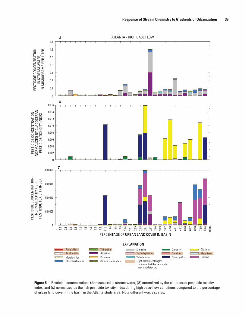
0
A
B
C
EXPLANATIONFungicidesAcetochlor
MetolachlorOther herbicides
TrifluralinAtrazinePrometonOther insecticides
SimazineTerbuthylazineTebuthiuron
CarbarylDieldrinChlorpyrifos
DiazinonMalathionFipronil
Light brown rectangles indicate that the pesticide was not detected
PEST
ICID
E CO
NCE
NTR
ATIO
NN
ORM
ALIZ
ED B
Y FI
SHPE
STIC
IDE
TOXI
CITY
INDE
X
PEST
ICID
E CO
NCE
NTR
ATIO
NN
ORM
ALIZ
ED B
Y CL
ADOC
ERAN
PEST
ICID
E TO
XICI
TY IN
DEX
PEST
ICID
E CO
NCE
NTR
ATIO
NIN
STR
EAM
WAT
ER,
IN M
ICRO
GRAM
S PE
R LI
TER
0
0
0
0.002
0.004
0.006
0.008
0.010
0.012
0.014
0.016
0.00005
0.00010
0.00015
0.00020
ATLANTA - HIGH BASE FLOW
0.2
0.4
0.6
0.8
1.0
1.2
1.4
2.3
2.8
3.6
3.8
4.5
4.8
4.9
5.9
7.3
11.0
13.4
16.4
17.8
20.4
22.1
22.9
24.8
25.1
25.7
35.6
38.3
39.7
42.6
43.1
43.2
60.6
66.2
67.0
72.5
85.4
100.
0
PERCENTAGE OF URBAN LAND COVER IN BASIN
Figure 5. Pesticide concentrations (A) measured in stream water, (B) normalized by the cladoceran pesticide toxicity index, and (C) normalized by the fish pesticide toxicity index during high base-flow conditions compared to the percentage of urban land cover in the basin in the Atlanta study area. Note different y-axis scales.
Response of Stream Chemistry to Gradients of Urbanization 39

Figure 6. Pesticide concentrations (A) measured in stream water, (B) normalized by the cladoceran pesticide toxicity index, and (C) normalized by the fish pesticide toxicity index during low base-flow conditions compared to the percentage of urban land cover in the basin in the Atlanta study area. Note different y-axis scales.
EXPLANATIONPERCENTAGE OF URBAN LAND COVER IN BASIN
TrifluralinAtrazinePrometonOther insecticides
SimazineTerbuthylazineTebuthiuron
CarbarylDieldrinChlorpyrifos
DiazinonMalathionFipronil
Light brown rectangles indicate that the pesticide was not detected
FungicidesAcetochlor
MetolachlorOther herbicides
PEST
ICID
E CO
NCE
NTR
ATIO
NN
ORM
ALIZ
ED B
Y FI
SHPE
STIC
IDE
TOXI
CITY
INDE
X
PEST
ICID
E CO
NCE
NTR
ATIO
NN
ORM
ALIZ
ED B
Y CL
ADOC
ERAN
PEST
ICID
E TO
XICI
TY IN
DEX
PEST
ICID
E CO
NCE
NTR
ATIO
NIN
STR
EAM
WAT
ER,
IN M
ICRO
GRAM
S PE
R LI
TER
0
0
0
0
0.1
0.2
0.3
0.4
0.01
0.02
0.03
0.04
0.05
0.0001
0.0002
0.0003
ATLANTA - LOW BASE FLOW
2.3
2.8
3.6
3.8
4.5
4.8
4.9
5.9
7.3
11.0
13.4
16.4
17.8
20.4
22.1
22.9
24.8
25.1
25.7
35.6
38.3
39.7
42.6
43.1
43.2
60.6
66.2
67.0
72.5
85.4
100.
0
A
B
C
40 Response of Stream Chemistry During Base Flow Across United States, 2002–04

Figure 7. Pesticide concentrations (A) measured in stream water, (B) normalized by the cladoceran pesticide toxicity index, and (C) normalized by the fish pesticide toxicity index during high base-flow conditions compared to the percentage of urban land cover in the basin in the Raleigh-Durham study area. Note different y-axis scales.
EXPLANATION
PEST
ICID
E CO
NCE
NTR
ATIO
NN
ORM
ALIZ
ED B
Y FI
SHPE
STIC
IDE
TOXI
CITY
INDE
X
PEST
ICID
E CO
NCE
NTR
ATIO
NN
ORM
ALIZ
ED B
Y CL
ADOC
ERAN
PEST
ICID
E TO
XICI
TY IN
DEX
PEST
ICID
E CO
NCE
NTR
ATIO
NIN
STR
EAM
WAT
ER,
IN M
ICRO
GRAM
S PE
R LI
TER
0
0
0
0
0.2
0.4
0.6
0.8
1.0
1.2
1.4
1.6
0.02
0.04
0.06
0.08
0.10
0.12
0.14
0.16
0.0002
0.0004
0.0006
0.0008
0.0010
RALEIGH-DURHAM - HIGH BASE FLOW
3.0
3.1
4.4
5.2
6.0
7.3
12.4
20.0
20.7
23.7
38.8
39.3
55.9
60.1
65.7
66.8
72.2
76.1
76.4
79.0
82.1
92.6
94.2
96.8
96.9
96.9
98.4
100.
0
PERCENTAGE OF URBAN LAND COVER IN BASIN
A
B
C
FungicidesAcetochlor
MetolachlorOther herbicides
TrifluralinAtrazinePrometonOther insecticides
SimazineTerbuthylazineTebuthiuron
CarbarylDieldrinChlorpyrifos
DiazinonMalathionFipronil
Light brown rectangles indicate that the pesticide was not detected
Response of Stream Chemistry to Gradients of Urbanization 41

Figure 8. Pesticide concentrations (A) measured in stream water, (B) normalized by the cladoceran pesticide toxicity index, and (C) normalized by the fish pesticide toxicity index during low base-flow conditions compared to the percentage of urban land cover in the basin in the Raleigh-Durham study area. Note different y-axis scales.
EXPLANATION
PEST
ICID
E CO
NCE
NTR
ATIO
NN
ORM
ALIZ
ED B
Y FI
SHPE
STIC
IDE
TOXI
CITY
INDE
XPE
STIC
IDE
CON
CEN
TRAT
ION
NOR
MAL
IZED
BY
CLAD
OCER
ANPE
STIC
IDE
TOXI
CITY
INDE
X
PEST
ICID
E CO
NCE
NTR
ATIO
NIN
STR
EAM
WAT
ER,
IN M
ICRO
GRAM
S PE
R LI
TER
0
0
0
0
0.2
0.4
0.6
0.8
0.05
0.10
0.15
0.20
0.25
0.0002
0.0004
0.0006
0.0008
0.0010
0.0012
0.0014
0.0016
RALEIGH-DURHAM - LOW BASE FLOW
3.0
3.1
4.4
5.2
6.0
7.3
18.2
20.0
20.0
20.7
23.7
38.8
39.3
44.3
53.0
55.9
60.1
65.7
66.8
72.2
76.1
76.4
79.0
82.1
92.6
94.2
96.8
96.9
96.9
98.4
100.
0
PERCENTAGE OF URBAN LAND COVER IN BASIN
A
B
C
FungicidesAcetochlor
MetolachlorOther herbicides
TrifluralinAtrazinePrometonOther insecticides
SimazineTerbuthylazineTebuthiuron
CarbarylDieldrinChlorpyrifos
DiazinonMalathionFipronil
Light brown rectangles indicate that the pesticide was not detected
42 Response of Stream Chemistry During Base Flow Across United States, 2002–04

Figure 9. Pesticide concentrations (A) measured in stream water, (B) normalized by the cladoceran pesticide toxicity index, and (C) normalized by the fish pesticide toxicity index during high base-flow conditions compared to the percentage of urban land cover in the basin in the Milwaukee-Green Bay study area. Note different y-axis scales.
EXPLANATION
PEST
ICID
E CO
NCE
NTR
ATIO
NN
ORM
ALIZ
ED B
Y FI
SHPE
STIC
IDE
TOXI
CITY
INDE
X
PEST
ICID
E CO
NCE
NTR
ATIO
NN
ORM
ALIZ
ED B
Y CL
ADOC
ERAN
PEST
ICID
E TO
XICI
TY IN
DEX
PEST
ICID
E CO
NCE
NTR
ATIO
NIN
STR
EAM
WAT
ER,
IN M
ICRO
GRAM
S PE
R LI
TER
0
0
0
4
2
6
8
10
12
14
0.0005
0.0010
0.0015
0.0020
0.0025
0.0030
0.0035
0
0.010
0.015
0.020
0.025
0.005
MILWAUKEE-GREEN BAY - HIGH BASE FLOW
3.2
3.5
3.7
4.0
4.4
5.0
5.0
5.4
5.5
5.7
7.4
11.7
13.8
14.9
16.3
17.6
20.2
24.4
27.3
30.4
58.8
62.9
68.9
78.0
86.0
87.2
92.8
97.6
99.1
100.
0
A
B
C
PERCENTAGE OF URBAN LAND COVER IN BASIN
FungicidesAcetochlor
MetolachlorOther herbicides
TrifluralinAtrazinePrometonOther insecticides
SimazineTerbuthylazineTebuthiuron
CarbarylDieldrinChlorpyrifos
DiazinonMalathionFipronil
Light brown rectangles indicate that the pesticide was not detected
Response of Stream Chemistry to Gradients of Urbanization 43

Figure 10. Pesticide concentrations (A) measured in stream water, (B) normalized by the cladoceran pesticide toxicity index, and (C) normalized by the fish pesticide toxicity index during low base-flow conditions compared to the percentage of urban land cover in the basin in the Milwaukee-Green Bay study area. Note different y-axis scales.
EXPLANATION
PEST
ICID
E CO
NCE
NTR
ATIO
NN
ORM
ALIZ
ED B
Y FI
SHPE
STIC
IDE
TOXI
CITY
INDE
X
PEST
ICID
E CO
NCE
NTR
ATIO
NN
ORM
ALIZ
ED B
Y CL
ADOC
ERAN
PEST
ICID
E TO
XICI
TY IN
DEX
PEST
ICID
E CO
NCE
NTR
ATIO
NIN
STR
EAM
WAT
ER,
IN M
ICRO
GRAM
S PE
R LI
TER
0
0
0.001
0.002
0.003
0.004
3.2
3.5
3.7
4.0
4.4
5.0
5.0
5.4
5.5
5.7
7.4
11.7
13.8
14.9
16.3
17.6
20.2
24.4
27.3
30.4
44.3
58.8
62.9
68.9
78.0
86.0
87.2
92.8
97.6
99.1
100.
0
0
0.1
0.2
0.3
0.4
0
0.2
0.4
0.6
0.8
1.0MILWAUKEE-GREEN BAY - LOW BASE FLOW
PERCENTAGE OF URBAN LAND COVER IN BASIN
A
B
C
FungicidesAcetochlor
MetolachlorOther herbicides
TrifluralinAtrazinePrometonOther insecticides
SimazineTerbuthylazineTebuthiuron
CarbarylDieldrinChlorpyrifos
DiazinonMalathionFipronil
Light brown rectangles indicate that the pesticide was not detected
44 Response of Stream Chemistry During Base Flow Across United States, 2002–04
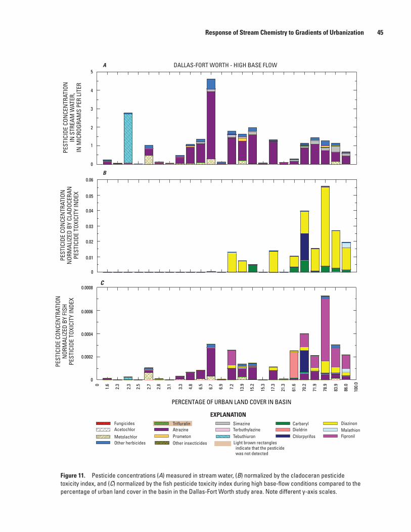
Figure 11. Pesticide concentrations (A) measured in stream water, (B) normalized by the cladoceran pesticide toxicity index, and (C) normalized by the fish pesticide toxicity index during high base-flow conditions compared to the percentage of urban land cover in the basin in the Dallas-Fort Worth study area. Note different y-axis scales.
EXPLANATION
PEST
ICID
E CO
NCE
NTR
ATIO
NN
ORM
ALIZ
ED B
Y FI
SHPE
STIC
IDE
TOXI
CITY
INDE
XPE
STIC
IDE
CON
CEN
TRAT
ION
NOR
MAL
IZED
BY
CLAD
OCER
ANPE
STIC
IDE
TOXI
CITY
INDE
X
PEST
ICID
E CO
NCE
NTR
ATIO
NIN
STR
EAM
WAT
ER,
IN M
ICRO
GRAM
S PE
R LI
TER
0
1.6
2.3
2.3
2.5
2.7
2.8
3.1
3.3
4.8
6.5
6.7
6.9
7.2
13.9
15.2
15.3
17.3
21.3
61.6
70.2
71.9
78.9
83.9
86.0
100.
0
0
0
0
1
2
3
4
5
0.01
0.02
0.03
0.04
0.05
0.06
0.0002
0.0004
0.0006
0.0008
DALLAS-FORT WORTH - HIGH BASE FLOW
PERCENTAGE OF URBAN LAND COVER IN BASIN
A
B
C
FungicidesAcetochlor
MetolachlorOther herbicides
TrifluralinAtrazinePrometonOther insecticides
SimazineTerbuthylazineTebuthiuron
CarbarylDieldrinChlorpyrifos
DiazinonMalathionFipronil
Light brown rectangles indicate that the pesticide was not detected
Response of Stream Chemistry to Gradients of Urbanization 45

Figure 12. Pesticide concentrations (A) measured in stream water, (B) normalized by the cladoceran pesticide toxicity index, and (C) normalized by the fish pesticide toxicity index during low base-flow conditions compared to the percentage of urban land cover in the basin in the Dallas-Fort Worth study area. Note different y-axis scales.
EXPLANATION
PEST
ICID
E CO
NCE
NTR
ATIO
NN
ORM
ALIZ
ED B
Y FI
SHPE
STIC
IDE
TOXI
CITY
INDE
X
PEST
ICID
E CO
NCE
NTR
ATIO
NN
ORM
ALIZ
ED B
Y CL
ADOC
ERAN
PEST
ICID
E TO
XICI
TY IN
DEX
PEST
ICID
E CO
NCE
NTR
ATIO
NIN
STR
EAM
WAT
ER,
IN M
ICRO
GRAM
S PE
R LI
TER
0
0
0
0
2
4
6
8
10
12
14
16
18
0.01
0.02
0.03
0.04
0.05
0.06
0.07
0.08
0.09
0.0005
0.0010
0.0015
0.0020
2.3
2.3
2.5
2.5
2.7
2.8
3.3
4.8
6.5
6.7
6.9
7.2
9.4
13.9
15.2
15.3
17.3
21.3
70.2
71.9
78.9
83.9
86.0
88.8
100.
0
DALLAS-FORT WORTH - LOW BASE FLOW
PERCENTAGE OF URBAN LAND COVER IN BASIN
A
B
C
FungicidesAcetochlor
MetolachlorOther herbicides
TrifluralinAtrazinePrometonOther insecticides
SimazineTerbuthylazineTebuthiuron
CarbarylDieldrinChlorpyrifos
DiazinonMalathionFipronil
Light brown rectangles indicate that the pesticide was not detected
46 Response of Stream Chemistry During Base Flow Across United States, 2002–04

Figure 13. Pesticide concentrations (A) measured in stream water, (B) normalized by the cladoceran pesticide toxicity index, and (C) normalized by the fish pesticide toxicity index during high base-flow conditions compared to the percentage of urban land cover in the basin in the Denver study area. Note different y-axis scales.
EXPLANATION
PEST
ICID
E CO
NCE
NTR
ATIO
NN
ORM
ALIZ
ED B
Y FI
SHPE
STIC
IDE
TOXI
CITY
INDE
X
PEST
ICID
E CO
NCE
NTR
ATIO
NN
ORM
ALIZ
ED B
Y CL
ADOC
ERAN
PEST
ICID
E TO
XICI
TY IN
DEX
PEST
ICID
E CO
NCE
NTR
ATIO
NIN
STR
EAM
WAT
ER,
IN M
ICRO
GRAM
S PE
R LI
TER
0
1.5
2.8
4.4
5.8
8.7
8.7
10.4
16.6
17.4
19.2
20.9
22.2
25.2
33.3
38.0
41.4
49.4
58.9
59.1
62.6
63.5
68.8
72.0
79.6
88.1
89.3
90.4
90.4
100.
0
0
0.00005
0.00011
0.00017
0.00023
0.00029
0.00035
0
0.02
0.04
0.06
0.08
0.10
0
0.1
0.2
0.3
0.4
0.5
0.6DENVER - HIGH BASE FLOW
PERCENTAGE OF URBAN LAND COVER IN BASIN
A
B
C
FungicidesAcetochlor
MetolachlorOther herbicides
TrifluralinAtrazinePrometonOther insecticides
SimazineTerbuthylazineTebuthiuron
CarbarylDieldrinChlorpyrifos
DiazinonMalathionFipronil
Light brown rectangles indicate that the pesticide was not detected
Response of Stream Chemistry to Gradients of Urbanization 47

Figure 14. Pesticide concentrations (A) measured in stream water, (B) normalized by the cladoceran pesticide toxicity index, and (C) normalized by the fish pesticide toxicity index during low base-flow conditions compared to the percentage of urban land cover in the basin in the Denver study area. Note different y-axis scales.
EXPLANATION
PEST
ICID
E CO
NCE
NTR
ATIO
NN
ORM
ALIZ
ED B
Y FI
SHPE
STIC
IDE
TOXI
CITY
INDE
X
PEST
ICID
E CO
NCE
NTR
ATIO
NN
ORM
ALIZ
ED B
Y CL
ADOC
ERAN
PEST
ICID
E TO
XICI
TY IN
DEX
PEST
ICID
E CO
NCE
NTR
ATIO
NIN
STR
EAM
WAT
ER,
IN M
ICRO
GRAM
S PE
R LI
TER
0
1.5
2.8
4.4
5.8
8.7
8.7
10.4
16.6
17.4
19.2
20.9
22.2
25.2
33.3
38.0
41.4
49.4
58.9
59.1
62.6
63.5
68.8
72.0
79.6
88.1
89.3
90.4
90.4
100.
0
0
0.0004
0.0002
0.0006
0.0008
0.0010
0.0012
0.0014
0.0016
0
0.05
0.10
0.15
0.20
0.25
0.30
0.6
1.2
1.8
2.4
3.0
3.6
0
DENVER - LOW BASE FLOW
PERCENTAGE OF URBAN LAND COVER IN BASIN
A
B
C
FungicidesAcetochlor
MetolachlorOther herbicides
TrifluralinAtrazinePrometonOther insecticides
SimazineTerbuthylazineTebuthiuron
CarbarylDieldrinChlorpyrifos
DiazinonMalathionFipronil
Light brown rectangles indicate that the pesticide was not detected
48 Response of Stream Chemistry During Base Flow Across United States, 2002–04
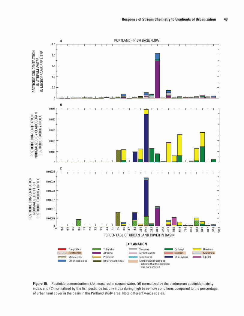
Figure 15. Pesticide concentrations (A) measured in stream water, (B) normalized by the cladoceran pesticide toxicity index, and (C) normalized by the fish pesticide toxicity index during high base-flow conditions compared to the percentage of urban land cover in the basin in the Portland study area. Note different y-axis scales.
EXPLANATION
PEST
ICID
E CO
NCE
NTR
ATIO
NN
ORM
ALIZ
ED B
Y FI
SHPE
STIC
IDE
TOXI
CITY
INDE
X
PEST
ICID
E CO
NCE
NTR
ATIO
NN
ORM
ALIZ
ED B
Y CL
ADOC
ERAN
PEST
ICID
E TO
XICI
TY IN
DEX
PEST
ICID
E CO
NCE
NTR
ATIO
NIN
STR
EAM
WAT
ER,
IN M
ICRO
GRAM
S PE
R LI
TER
0 0.2
0.4
0.5
0.6
1.9
2.3
3.3
3.5
4.4
7.1
7.5
8.6
13.2
19.0
22.0
27.1
28.2
33.0
37.6
41.9
59.5
61.9
72.4
81.0
82.9
84.3
88.7
97.8
100.
00
0.00005
0.00011
0.00017
0.00023
0.00029
0.00035
0
0.005
0.010
0.015
0.020
0.025
0
0.5
1.0
1.5
2.0
2.5PORTLAND - HIGH BASE FLOW
PERCENTAGE OF URBAN LAND COVER IN BASIN
A
B
C
FungicidesAcetochlor
MetolachlorOther herbicides
TrifluralinAtrazinePrometonOther insecticides
SimazineTerbuthylazineTebuthiuron
CarbarylDieldrinChlorpyrifos
DiazinonMalathionFipronil
Light brown rectangles indicate that the pesticide was not detected
Response of Stream Chemistry to Gradients of Urbanization 49

Figure 16. Pesticide concentrations (A) measured in stream water, (B) normalized by the cladoceran pesticide toxicity index, and (C) normalized by the fish pesticide toxicity index during low base-flow conditions compared to the percentage of urban land cover in the basin in the Portland study area. Note different y-axis scales.
EXPLANATION
PEST
ICID
E CO
NCE
NTR
ATIO
NN
ORM
ALIZ
ED B
Y FI
SHPE
STIC
IDE
TOXI
CITY
INDE
X
PEST
ICID
E CO
NCE
NTR
ATIO
NN
ORM
ALIZ
ED B
Y CL
ADOC
ERAN
PEST
ICID
E TO
XICI
TY IN
DEX
PEST
ICID
E CO
NCE
NTR
ATIO
NIN
STR
EAM
WAT
ER,
IN M
ICRO
GRAM
S PE
R LI
TER
0 0.2
0.4
0.5
0.6
1.9
2.3
3.3
3.5
4.4
7.1
7.5
8.6
13.2
19.0
22.0
27.1
28.2
33.0
37.6
41.9
59.5
61.9
72.4
82.9
88.7
100.
0
81.0
84.3
97.8
0
0.00002
0.00004
0.00006
0.00008
0.00010
0.00012
0.00014
0
0.005
0.010
0.015
0.020
0.025
0
0.05
0.10
0.15
0.20
0.25PORTLAND - LOW BASE FLOW
PERCENTAGE OF URBAN LAND COVER IN BASIN
A
B
C
FungicidesAcetochlor
MetolachlorOther herbicides
TrifluralinAtrazinePrometonOther insecticides
SimazineTerbuthylazineTebuthiuron
CarbarylDieldrinChlorpyrifos
DiazinonMalathionFipronil
Light brown rectangles indicate that the pesticide was not detected
50 Response of Stream Chemistry During Base Flow Across United States, 2002–04
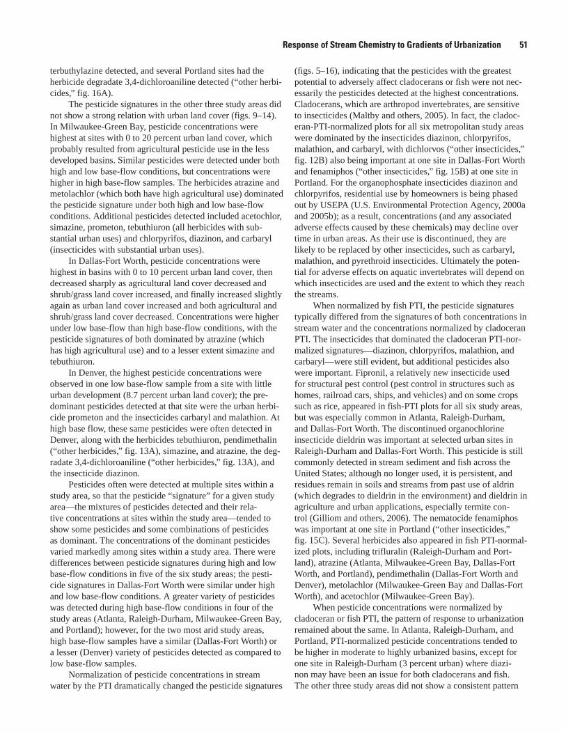
terbuthylazine detected, and several Portland sites had the herbicide degradate 3,4-dichloroaniline detected (“other herbi-cides,” fig. 16A).
The pesticide signatures in the other three study areas did not show a strong relation with urban land cover (figs. 9–14). In Milwaukee-Green Bay, pesticide concentrations were highest at sites with 0 to 20 percent urban land cover, which probably resulted from agricultural pesticide use in the less developed basins. Similar pesticides were detected under both high and low base-flow conditions, but concentrations were higher in high base-flow samples. The herbicides atrazine and metolachlor (which both have high agricultural use) dominated the pesticide signature under both high and low base-flow conditions. Additional pesticides detected included acetochlor, simazine, prometon, tebuthiuron (all herbicides with sub-stantial urban uses) and chlorpyrifos, diazinon, and carbaryl (insecticides with substantial urban uses).
In Dallas-Fort Worth, pesticide concentrations were highest in basins with 0 to 10 percent urban land cover, then decreased sharply as agricultural land cover decreased and shrub/grass land cover increased, and finally increased slightly again as urban land cover increased and both agricultural and shrub/grass land cover decreased. Concentrations were higher under low base-flow than high base-flow conditions, with the pesticide signatures of both dominated by atrazine (which has high agricultural use) and to a lesser extent simazine and tebuthiuron.
In Denver, the highest pesticide concentrations were observed in one low base-flow sample from a site with little urban development (8.7 percent urban land cover); the pre-dominant pesticides detected at that site were the urban herbi-cide prometon and the insecticides carbaryl and malathion. At high base flow, these same pesticides were often detected in Denver, along with the herbicides tebuthiuron, pendimethalin (“other herbicides,” fig. 13A), simazine, and atrazine, the deg-radate 3,4-dichloroaniline (“other herbicides,” fig. 13A), and the insecticide diazinon.
Pesticides often were detected at multiple sites within a study area, so that the pesticide “signature” for a given study area—the mixtures of pesticides detected and their rela-tive concentrations at sites within the study area—tended to show some pesticides and some combinations of pesticides as dominant. The concentrations of the dominant pesticides varied markedly among sites within a study area. There were differences between pesticide signatures during high and low base-flow conditions in five of the six study areas; the pesti-cide signatures in Dallas-Fort Worth were similar under high and low base-flow conditions. A greater variety of pesticides was detected during high base-flow conditions in four of the study areas (Atlanta, Raleigh-Durham, Milwaukee-Green Bay, and Portland); however, for the two most arid study areas, high base-flow samples have a similar (Dallas-Fort Worth) or a lesser (Denver) variety of pesticides detected as compared to low base-flow samples.
Normalization of pesticide concentrations in stream water by the PTI dramatically changed the pesticide signatures
(figs. 5–16), indicating that the pesticides with the greatest potential to adversely affect cladocerans or fish were not nec-essarily the pesticides detected at the highest concentrations. Cladocerans, which are arthropod invertebrates, are sensitive to insecticides (Maltby and others, 2005). In fact, the cladoc-eran-PTI-normalized plots for all six metropolitan study areas were dominated by the insecticides diazinon, chlorpyrifos, malathion, and carbaryl, with dichlorvos (“other insecticides,” fig. 12B) also being important at one site in Dallas-Fort Worth and fenamiphos (“other insecticides,” fig. 15B) at one site in Portland. For the organophosphate insecticides diazinon and chlorpyrifos, residential use by homeowners is being phased out by USEPA (U.S. Environmental Protection Agency, 2000a and 2005b); as a result, concentrations (and any associated adverse effects caused by these chemicals) may decline over time in urban areas. As their use is discontinued, they are likely to be replaced by other insecticides, such as carbaryl, malathion, and pyrethroid insecticides. Ultimately the poten-tial for adverse effects on aquatic invertebrates will depend on which insecticides are used and the extent to which they reach the streams.
When normalized by fish PTI, the pesticide signatures typically differed from the signatures of both concentrations in stream water and the concentrations normalized by cladoceran PTI. The insecticides that dominated the cladoceran PTI-nor-malized signatures—diazinon, chlorpyrifos, malathion, and carbaryl—were still evident, but additional pesticides also were important. Fipronil, a relatively new insecticide used for structural pest control (pest control in structures such as homes, railroad cars, ships, and vehicles) and on some crops such as rice, appeared in fish-PTI plots for all six study areas, but was especially common in Atlanta, Raleigh-Durham, and Dallas-Fort Worth. The discontinued organochlorine insecticide dieldrin was important at selected urban sites in Raleigh-Durham and Dallas-Fort Worth. This pesticide is still commonly detected in stream sediment and fish across the United States; although no longer used, it is persistent, and residues remain in soils and streams from past use of aldrin (which degrades to dieldrin in the environment) and dieldrin in agriculture and urban applications, especially termite con-trol (Gilliom and others, 2006). The nematocide fenamiphos was important at one site in Portland (“other insecticides,” fig. 15C). Several herbicides also appeared in fish PTI-normal-ized plots, including trifluralin (Raleigh-Durham and Port-land), atrazine (Atlanta, Milwaukee-Green Bay, Dallas-Fort Worth, and Portland), pendimethalin (Dallas-Fort Worth and Denver), metolachlor (Milwaukee-Green Bay and Dallas-Fort Worth), and acetochlor (Milwaukee-Green Bay).
When pesticide concentrations were normalized by cladoceran or fish PTI, the pattern of response to urbanization remained about the same. In Atlanta, Raleigh-Durham, and Portland, PTI-normalized pesticide concentrations tended to be higher in moderate to highly urbanized basins, except for one site in Raleigh-Durham (3 percent urban) where diazi-non may have been an issue for both cladocerans and fish. The other three study areas did not show a consistent pattern
Response of Stream Chemistry to Gradients of Urbanization 51

of response to urban land cover. In Dallas-Fort Worth and Denver, high base-flow samples showed higher PTI-normal-ized pesticide concentrations in moderate-to-highly urbanized basins, but low base-flow samples did not. At low base-flow in Milwaukee-Green Bay, Dallas-Fort Worth, and Denver, a single site with less than 10 percent urban land cover had the highest PTI-normalized pesticide concentrations; the high relative potential toxicity largely was due to the insecticides chlorpyrifos, diazinon, malathion, and carbaryl.
The PTI is designed to indicate relative potential toxicity; it cannot be used to evaluate whether actual toxicity is occur-ring. Nonetheless, PTI-normalization provides information on which pesticides may be most important from a toxicity perspective to aquatic organisms in the streams sampled.
Suspended SedimentIn all six study areas, the relation between suspended-
sediment concentrations and the percentage of urban land cover in the basin was weak during high and low base-flow conditions (fig. 17A). The highest concentrations of sus-pended sediment were not consistently present in more urbanized basins. Maximum suspended-sediment concentra-tions occurred during high base-flow conditions in four study areas (Atlanta, Milwaukee-Green Bay, Dallas-Fort Worth, and Denver), during low base-flow conditions in one study area (Raleigh-Durham), and during both high and low base-flow conditions in one study area (Portland).
For the most part, relations between suspended-sediment concentrations and urban and landscape variables were weak in all six study areas (table 5A). In Atlanta, suspended-sedi-ment concentrations were positively related to the distance from the stream to the nearest road. In Atlanta and Dallas-Fort Worth, suspended-sediment concentrations were positively related to the percentage of wetlands in the basin and buffer; fine particles, such as silt and clays, may have been mobilized from wetland sediment deposits. In Milwaukee-Green Bay and Denver, suspended-sediment concentrations were negatively related to a measure of housing age. In older communities in Denver, more mature vegetative cover and lack of surface disturbance from new construction may have contributed to a decrease in the amount of sediment in runoff (Sprague and others, 2006). Likewise, well-established lawns and low-inten-sity traffic along streets of older, nonurban, residential areas in Milwaukee-Green Bay may have led to relatively smaller amounts of sediment in runoff. In Portland, suspended-sedi-ment concentrations were negatively related to the percentage of shrub/grass land cover in the basin and buffer, sand content in the soil, and depth to the water table, and positively related to soil erodibility. The depth to the water table likely is great-est beneath upland areas in the stream headwaters; land use in these areas was typically forested and shrub/grass land. Forest and shrub/grass land may have been more resistant to erosion than agricultural or urban land, resulting in decreas-ing suspended-sediment concentrations as the percentage of forested or shrub/grass land area, or both, increased. Rainfall
and snowmelt may have infiltrated readily through sandy soils, reducing the intensity of surface runoff and associated sedi-ment transport in these urbanizing basins in Portland.
The results for suspended-sediment concentrations from this study support previous research indicating that strategies to control sediment transport to streams in urbanizing areas may need to focus on conditions during stormwater runoff to a greater degree than conditions during base flow. Base flow has been found to transport only about 1 percent of the annual suspended-sediment load in streams, whereas stormwater run-off typically transports the remaining 99 percent (Landers and others, 2002). As a result, management strategies may be most effective when considering factors related to runoff generation.
SulfateIn Atlanta, the relation between sulfate concentrations
and the percentage of urban land cover in the basin was strong during high and low base-flow conditions (fig. 17B). Sulfate concentrations increased as most measures of urban-ization—including housing density, road density, population density, patch size and homogeneity of urban land area, urban land cover in the basin and buffer, and impervious area in the basin and buffer—increased (table 5B). Sulfate concentrations decreased as a measure of housing age increased. Relations with sulfate concentrations generally were stronger with the urban variables than with the landscape variables. Two notable exceptions were the negative relation with the percentage of shrub/grass land cover in the basin and buffer during high and low base-flow conditions and the negative relation with the percentage of agricultural land cover in the basin during high base-flow conditions. These relations likely reflect a decrease in background forested land cover as urban land cover increased (fig. 2).
In Raleigh-Durham, the relation between sulfate concen-trations and the percentage of urban land cover in the basin also was strong during high and low base-flow conditions (fig. 17B). Sulfate concentrations increased as most measures of urbanization—including housing density, road density, popula-tion density, patch size and homogeneity of urban land area, urban land cover in the basin and buffer, impervious area in the basin and buffer, and housing age—increased (table 5B). Sulfate concentrations generally decreased with increasing distance from the stream to the nearest road. In addition to the urban variables, there were several strong relations between sulfate concentrations and landscape variables. During high and low base-flow conditions, sulfate concentrations gener-ally decreased as the percentage of agricultural, shrub/grass, wetland land cover in the basin and buffer, and soil erod-ibility increased. These relations likely reflect a decrease in background forested land cover and an increase in impervious surface area as urban land cover increased (fig. 2).
In Milwaukee-Green Bay, the relation between sulfate concentrations and the percentage of urban land cover in the basin was strong (fig. 17B). Sulfate concentrations increased as most measures of urbanization—including housing density,
52 Response of Stream Chemistry During Base Flow Across United States, 2002–04

Figure 17. (A) Suspended-sediment, (B) dissolved sulfate, and (C) dissolved chloride concentrations during high and low base flow compared to the percentage of urban land cover in the basin in the Atlanta, Raleigh-Durham, Milwaukee-Green Bay, Dallas-Fort Worth, Denver, and Portland study areas.
EXPLANATIONHigh base-flow sample
Low base-flow sampleLOWESS smooth line (high base-flow sample)
LOWESS smooth line(low base-flow sample)
Spearman’s rankcorrelation coefficient(high base-flow sample)
Spearman’s rankcorrelation coefficent(low base-flow sample)
ATLANTA RALEIGH-DURHAMMILWAUKEE-GREEN BAY
DALLAS-FORT WORTH DENVER PORTLAND
DISS
OLVE
D CH
LORI
DE
CON
CEN
TRAT
ION
, IN
MIL
LIGR
AMS
PER
LITE
R
DISS
OLVE
D SU
LFAT
E CO
NCE
NTR
ATIO
N, I
N
MIL
LIGR
AMS
PER
LITE
R
SUSP
ENDE
D-SE
DIM
ENT
CON
CEN
TRAT
ION
, IN
M
ILLI
GRAM
S PE
R LI
TER
PERCENTAGE OF URBAN LAND COVER IN BASIN
0.10
0.19
350
300100
50
0
0
0
50
100
150400
500
0
50
100
150400
500
0
50
100
150400
500
0
50
100
150400
500
0
50
100
150400
500
0
100
200
300
400
500
50
1001,500
1,600
0 0
200
400
600
8001,000
1,200
1,4001,600
0200
400600800
1,000
1,2001,400
1,600
0
200
400600
800
1,000
1,200
1,4001,600
50
1001,500
1,600
0
50
1001,500
1,600
350
300100
50
0
350
300100
50
00
50
100
150
200
250
300
350
0
50
100
150
200
250
300
350
0
50
100
150
200
250
300
350-0.32
0 20 40 60 80 100 0 20 40 60 80 100 0 20 40 60 80 100 0 20 40 60 80 100 0 20 40 60 80 100 0 20 40 60 80 100
0 20 40 60 80 100 0 20 40 60 80 100 0 20 40 60 80 100 0 20 40 60 80 100 0 20 40 60 80 100 0 20 40 60 80 100
0 20 40 60 80 100 0 20 40 60 80 100 0 20 40 60 80 100 0 20 40 60 80 100 0 20 40 60 80 100 0 20 40 60 80 100
0.07
0.83 0.85
0.84 0.82 0.69 0.66 0.85 0.71 0.18 0.53 0.25 0.56 0.62 0.49
0.81 0.82 0.63 0.37 0.04 0.24 -0.03 0.13 0.76 0.57
-0.18 0.07 0.41 0.22 -0.24 0.15 0.11 0.23 0.30 0.44
B
C
A
Response of Stream Chem
istry to Gradients of Urbanization
53

Table 5. Spearman’s rank correlations between (A) suspended-sediment concentrations, (B) dissolved sulfate concentrations, and (C) dissolved chloride concentrations during high and low base flow and selected urban and landscape variables.
[Values in bold are significantly different during high and low base-flow conditions. HUDEN, 2000 housing unit density; ROADDEN, road density; POPDENKM, 2000 population density; LPI_2, larg-est urban patch index; PLA_2, percentage of like adjacencies (urban); P_NLCD1_2, percentage of urban land cover in basin; P_NLCD1_B2, percentage of urban land cover in buffer; NLCD_IS, mean percent impervious surface in basin; NLCD_BIS, mean percent impervious surface in buffer; PHU_G60, percentage of housing units built prior to 1939; SEG_RMD, mean distance from stream segment to nearest road; SLOPE_X, mean basin slope; P_NLCD1_8, percentage of herbaceous planted/cultivated land cover in basin; P_NLCD1_B8, percentage of herbaceous planted/cultivated land cover in buf-fer; P_NLCD1_5, percentage of shrub/grass land cover in basin; P_NLCD1_B5, percentage of shrub/grass land cover in buffer; P_NLCD1_9, percentage of wetland land cover in basin; P_NLCD1_B9, percentage of wetland land cover in buffer; WET_MEAN, mean value of wetness index across all cells in basin; SNDH, mean high-range sand (soil); WTDH, mean high-range depth to water table; KFCAVE, mean soil erodibility factor (K factor)]
(A) Suspended-sediment concentrations
Variable code
Variable short name
High base flow Low base flow
AtlantaRa-
leigh-Durham
Mil-waukee-
Green Bay
Dallas-Fort
WorthDenver Portland Atlanta
Raleigh-Durham
Mil-waukee-
Green Bay
Dallas-Fort
WorthDenver Portland
Urban variables
HUDEN Housing density -0.38 -0.15 0.46 -0.31 -0.09 0.36 0.07 0.11 0.21 0.31 0.08 0.58
ROADDEN Road density -0.38 -0.18 0.42 -0.25 0.03 0.35 0.05 0.08 0.18 0.24 0.22 0.42
POPDENKM Population density -0.40 -0.12 0.42 -0.27 -0.05 0.36 0.12 0.15 0.21 0.25 0.13 0.52
LPI_2Patch size of urban
land area-0.30 -0.18 0.35 -0.22 0.11 0.28 0.08 0.05 0.17 0.11 0.24 0.50
PLA_2Homogeneity of urban
land area-0.27 -0.20 0.36 -0.18 0.09 0.32 0.16 0.10 0.18 0.16 0.15 0.53
P_NLCD1_2Urban land cover in
basin-0.32 -0.18 0.41 -0.24 0.11 0.30 0.07 0.07 0.22 0.15 0.23 0.44
P_NLCD1_B2Urban land cover in
buffer-0.28 -0.21 0.35 -0.34 0.13 0.30 0.07 0.05 0.12 0.25 0.18 0.48
NLCD_ISImpervious area in
basin-0.33 -0.14 0.35 -0.24 0.11 0.30 0.07 0.18 0.15 0.18 0.22 0.45
NLCD_BISImpervious area in
buffer-0.30 -0.13 0.27 -0.29 0.13 0.32 0.08 0.10 0.08 0.28 0.14 0.49
PHU_G60 Housing age 0.20 -0.35 -0.64 0.34 -0.33 -0.02 -0.10 -0.39 -0.35 -0.28 -0.62 -0.40
SEG_RMDDistance from stream
to nearest road0.57 0.25 -0.11 0.20 0.09 -0.35 0.18 0.32 -0.08 -0.28 -0.04 -0.23
Landscape variables
SLOPE_X Basin slope -0.57 0.36 -0.03 -0.37 -0.11 -0.10 -0.34 0.30 -0.06 -0.13 -0.21 -0.31
P_NLCD1_8Agricultural land
cover in basin0.32 0.24 -0.39 0.45 -0.04 0.01 0.14 0.01 -0.22 -0.05 -0.07 0.19
54
Response of Stream Chem
istry During Base Flow Across United States, 2002–04

Table 5. Spearman’s rank correlations between (A) suspended-sediment concentrations, (B) dissolved sulfate concentrations, and (C) dissolved chloride concentrations during high and low base flow and selected urban and landscape variables.—Continued
[Values in bold are significantly different during high and low base-flow conditions. HUDEN, 2000 housing unit density; ROADDEN, road density; POPDENKM, 2000 population density; LPI_2, larg-est urban patch index; PLA_2, percentage of like adjacencies (urban); P_NLCD1_2, percentage of urban land cover in basin; P_NLCD1_B2, percentage of urban land cover in buffer; NLCD_IS, mean percent impervious surface in basin; NLCD_BIS, mean percent impervious surface in buffer; PHU_G60, percentage of housing units built prior to 1939; SEG_RMD, mean distance from stream segment to nearest road; SLOPE_X, mean basin slope; P_NLCD1_8, percentage of herbaceous planted/cultivated land cover in basin; P_NLCD1_B8, percentage of herbaceous planted/cultivated land cover in buf-fer; P_NLCD1_5, percentage of shrub/grass land cover in basin; P_NLCD1_B5, percentage of shrub/grass land cover in buffer; P_NLCD1_9, percentage of wetland land cover in basin; P_NLCD1_B9, percentage of wetland land cover in buffer; WET_MEAN, mean value of wetness index across all cells in basin; SNDH, mean high-range sand (soil); WTDH, mean high-range depth to water table; KFCAVE, mean soil erodibility factor (K factor)]
(A) Suspended-sediment concentrations
Variable code
Variable short name
High base flow Low base flow
AtlantaRa-
leigh-Durham
Mil-waukee-
Green Bay
Dallas-Fort
WorthDenver Portland Atlanta
Raleigh-Durham
Mil-waukee-
Green Bay
Dallas-Fort
WorthDenver Portland
Landscape variables
P_NLCD1_B8Agricultural land
cover in buffer0.27 0.30 -0.46 0.39 -0.05 0.09 0.16 -0.13 -0.29 -0.10 -0.12 0.12
P_NLCD1_5Shrub/grass land cover
in basin0.09 0.27 0.31 0.17 -0.14 -0.20 -0.07 -0.12 0.23 -0.02 -0.23 -0.47
P_NLCD1_B5Shrub/grass land cover
in buffer0.12 0.36 0.28 0.35 -0.35 -0.28 -0.09 -0.08 0.11 -0.06 -0.19 -0.56
P_NLCD1_9Wetland land cover in
basin0.62 0.35 -0.29 0.47 -0.15 0.26 0.37 0.30 0.03 0.14 -0.26 -0.04
P_NLCD1_B9Wetland land cover in
buffer0.53 0.32 -0.16 0.60 -0.18 0.25 0.34 0.28 0.18 0.10 -0.23 -0.04
WET_MEAN Basin-wetness index 0.49 -0.19 0.01 0.25 0.12 0.14 0.33 -0.28 -0.02 0.30 0.12 0.27
SNDH Sand content in soil -0.01 -0.10 -0.03 0.03 -0.08 -0.53 0.33 0.28 -0.22 -0.33 0.03 -0.65
WTDH Depth to water table 0.10 -0.17 0.08 0.00 0.03 -0.61 0.16 0.13 -0.15 0.43 0.05 -0.53
KFCAVE Soil erodibility 0.32 0.26 0.01 0.13 0.36 0.42 0.09 -0.06 0.26 -0.42 0.46 0.67
Response of Stream Chem
istry to Gradients of Urbanization
55

Table 5. Spearman’s rank correlations between (A) suspended-sediment concentrations, (B) dissolved sulfate concentrations, and (C) dissolved chloride concentrations during high and low base flow and selected urban and landscape variables.—Continued
[Values in bold are significantly different during high and low base-flow conditions. HUDEN, 2000 housing unit density; ROADDEN, road density; POPDENKM, 2000 population density; LPI_2, largest urban patch index; PLA_2, percentage of like adjacencies (urban); P_NLCD1_2, percentage of urban land cover in basin; P_NLCD1_B2, percentage of urban land cover in buffer; NLCD_IS, mean percent impervious surface in basin; NLCD_BIS, mean percent impervious surface in buffer; PHU_G60, percentage of housing units built prior to 1939; SEG_RMD, mean distance from stream segment to nearest road; SLOPE_X, mean basin slope; P_NLCD1_8, percentage of herbaceous planted/cultivated land cover in basin; P_NLCD1_B8, percentage of herbaceous planted/cultivated land cover in buffer; P_NLCD1_5, percentage of shrub/grass land cover in basin; P_NLCD1_B5, percentage of shrub/grass land cover in buffer; P_NLCD1_9, percentage of wetland land cover in basin; P_NLCD1_B9, percentage of wetland land cover in buffer; WET_MEAN, mean value of wetness index across all cells in basin; SNDH, mean high-range sand (soil); WTDH, mean high-range depth to water table; KFCAVE, mean soil erodibility factor (K factor)]
(B) Dissolved sulfate concentrations
Variable code
Variable short name
High base flow Low base flow
AtlantaRaleigh-Durham
Mil-waukee-
Green Bay
Dallas-Fort
Worth Denver Portland AtlantaRaleigh-Durham
Mil-waukee-
Green Bay
Dallas-Fort
Worth Denver Portland
Urban variables
HUDEN Housing density 0.80 0.70 0.61 0.02 -0.10 0.78 0.84 0.71 0.33 0.22 -0.06 0.57
ROADDEN Road density 0.79 0.78 0.53 0.08 -0.09 0.70 0.82 0.80 0.24 0.29 0.08 0.56
POPDENKM Population density 0.80 0.70 0.61 0.00 -0.06 0.76 0.83 0.72 0.31 0.25 0.03 0.56
LPI_2Patch size of urban
land area0.83 0.80 0.57 -0.03 -0.02 0.79 0.85 0.82 0.32 0.22 0.11 0.57
PLA_2Homogeneity of
urban land area0.83 0.82 0.63 -0.01 -0.04 0.78 0.84 0.82 0.38 0.20 0.00 0.58
P_NLCD1_2Urban land cover in
basin0.83 0.81 0.63 0.04 -0.03 0.76 0.85 0.82 0.37 0.24 0.13 0.57
P_NLCD1_B2Urban land cover in
buffer0.83 0.85 0.53 -0.03 -0.10 0.77 0.86 0.84 0.25 0.13 0.06 0.56
NLCD_ISImpervious area in
basin0.82 0.87 0.65 -0.02 -0.02 0.77 0.85 0.83 0.36 0.23 0.12 0.59
NLCD_BISImpervious area in
buffer0.82 0.88 0.61 -0.12 -0.14 0.78 0.87 0.82 0.31 0.07 0.02 0.58
PHU_G60 Housing age -0.70 0.51 -0.69 -0.16 -0.32 -0.52 -0.77 0.50 -0.43 -0.23 -0.43 -0.49
SEG_RMDDistance from stream
to nearest road-0.45 -0.50 -0.18 0.21 -0.05 -0.14 -0.52 -0.61 -0.14 0.05 -0.03 -0.07
Landscape variables
SLOPE_X Basin slope -0.24 -0.26 -0.52 -0.03 -0.30 -0.52 -0.08 -0.29 -0.21 -0.19 -0.61 -0.38
P_NLCD1_8Agricultural land
cover in basin-0.68 -0.59 -0.35 0.03 0.09 -0.22 -0.47 -0.62 -0.20 0.10 0.17 -0.22
56
Response of Stream Chem
istry During Base Flow Across United States, 2002–04
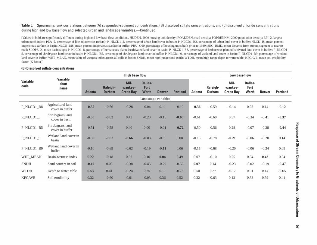
Table 5. Spearman’s rank correlations between (A) suspended-sediment concentrations, (B) dissolved sulfate concentrations, and (C) dissolved chloride concentrations during high and low base flow and selected urban and landscape variables.—Continued
[Values in bold are significantly different during high and low base-flow conditions. HUDEN, 2000 housing unit density; ROADDEN, road density; POPDENKM, 2000 population density; LPI_2, largest urban patch index; PLA_2, percentage of like adjacencies (urban); P_NLCD1_2, percentage of urban land cover in basin; P_NLCD1_B2, percentage of urban land cover in buffer; NLCD_IS, mean percent impervious surface in basin; NLCD_BIS, mean percent impervious surface in buffer; PHU_G60, percentage of housing units built prior to 1939; SEG_RMD, mean distance from stream segment to nearest road; SLOPE_X, mean basin slope; P_NLCD1_8, percentage of herbaceous planted/cultivated land cover in basin; P_NLCD1_B8, percentage of herbaceous planted/cultivated land cover in buffer; P_NLCD1_5, percentage of shrub/grass land cover in basin; P_NLCD1_B5, percentage of shrub/grass land cover in buffer; P_NLCD1_9, percentage of wetland land cover in basin; P_NLCD1_B9, percentage of wetland land cover in buffer; WET_MEAN, mean value of wetness index across all cells in basin; SNDH, mean high-range sand (soil); WTDH, mean high-range depth to water table; KFCAVE, mean soil erodibility factor (K factor)]
(B) Dissolved sulfate concentrations
Variable code
Variable short name
High base flow Low base flow
AtlantaRaleigh-Durham
Mil-waukee-
Green Bay
Dallas-Fort
Worth Denver Portland AtlantaRaleigh-Durham
Mil-waukee-
Green Bay
Dallas-Fort
Worth Denver Portland
Landscape variables
P_NLCD1_B8Agricultural land
cover in buffer-0.52 -0.56 -0.28 -0.04 0.11 -0.10 -0.36 -0.59 -0.14 0.03 0.14 -0.12
P_NLCD1_5Shrub/grass land
cover in basin-0.63 -0.62 0.43 -0.23 -0.16 -0.63 -0.61 -0.60 0.37 -0.34 -0.41 -0.37
P_NLCD1_B5Shrub/grass land
cover in buffer-0.51 -0.58 0.40 0.00 -0.01 -0.72 -0.50 -0.56 0.28 -0.07 -0.28 -0.44
P_NLCD1_9Wetland land cover in
basin-0.08 -0.83 -0.66 -0.03 -0.06 0.08 -0.15 -0.78 -0.21 -0.06 -0.20 0.14
P_NLCD1_B9Wetland land cover in
buffer-0.10 -0.69 -0.62 -0.19 -0.11 0.06 -0.15 -0.68 -0.20 -0.06 -0.24 0.09
WET_MEAN Basin-wetness index 0.22 -0.18 0.57 0.10 0.04 0.49 0.07 -0.10 0.25 0.34 0.43 0.34
SNDH Sand content in soil -0.12 0.08 -0.38 -0.45 -0.29 -0.56 0.07 0.14 -0.23 -0.02 -0.19 -0.47
WTDH Depth to water table 0.53 0.41 -0.24 0.25 0.11 -0.78 0.50 0.37 -0.17 0.01 0.14 -0.65
KFCAVE Soil erodibility 0.32 -0.60 -0.01 -0.03 0.36 0.52 0.32 -0.63 0.12 0.33 0.59 0.41
Response of Stream Chem
istry to Gradients of Urbanization
57

Table 5. Spearman’s rank correlations between (A) suspended-sediment concentrations, (B) dissolved sulfate concentrations, and (C) dissolved chloride concentrations during high and low base flow and selected urban and landscape variables.—Continued
[Values in bold are significantly different during high and low base-flow conditions. HUDEN, 2000 housing unit density; ROADDEN, road density; POPDENKM, 2000 population density; LPI_2, larg-est urban patch index; PLA_2, percentage of like adjacencies (urban); P_NLCD1_2, percentage of urban land cover in basin; P_NLCD1_B2, percentage of urban land cover in buffer; NLCD_IS, mean percent impervious surface in basin; NLCD_BIS, mean percent impervious surface in buffer; PHU_G60, percentage of housing units built prior to 1939; SEG_RMD, mean distance from stream segment to nearest road; SLOPE_X, mean basin slope; P_NLCD1_8, percentage of herbaceous planted/cultivated land cover in basin; P_NLCD1_B8, percentage of herbaceous planted/cultivated land cover in buffer; P_NLCD1_5, percentage of shrub/grass land cover in basin; P_NLCD1_B5, percentage of shrub/grass land cover in buffer; P_NLCD1_9, percentage of wetland land cover in basin; P_NLCD1_B9, percent-age of wetland land cover in buffer; WET_MEAN, mean value of wetness index across all cells in basin; SNDH, mean high-range sand (soil); WTDH, mean high-range depth to water table; KFCAVE, mean soil erodibility factor (K factor)]
(C) Dissolved chloride concentrations
Variable code
Variable short name
High base flow Low base flow
AtlantaRaleigh-Durham
Mil-waukee-
Green Bay
Dallas-Fort
WorthDenver Portland Atlanta
Raleigh-Durham
Mil-waukee-
Green Bay
Dallas-Fort
WorthDenver Portland
Urban variablesHUDEN Housing density 0.84 0.59 0.84 0.19 0.25 0.71 0.78 0.51 0.66 0.48 0.48 0.54ROADDEN Road density 0.84 0.66 0.81 0.15 0.20 0.56 0.76 0.63 0.68 0.51 0.51 0.46POPDENKM Population density 0.82 0.58 0.82 0.14 0.25 0.66 0.77 0.51 0.66 0.48 0.52 0.51
LPI_2Patch size of urban land
area0.83 0.69 0.81 0.09 0.26 0.69 0.82 0.65 0.72 0.48 0.58 0.54
PLA_2Homogeneity of urban
land area0.80 0.72 0.85 0.04 0.28 0.72 0.83 0.65 0.69 0.43 0.55 0.54
P_NLCD1_2Urban land cover in
basin0.84 0.69 0.85 0.18 0.25 0.62 0.82 0.66 0.71 0.53 0.56 0.49
P_NLCD1_B2Urban land cover in
buffer0.81 0.69 0.76 0.18 0.14 0.66 0.80 0.66 0.60 0.48 0.47 0.51
NLCD_IS Impervious area in basin 0.81 0.76 0.87 0.07 0.24 0.64 0.81 0.66 0.70 0.47 0.55 0.50
NLCD_BISImpervious area in
buffer0.80 0.77 0.82 0.09 0.10 0.68 0.81 0.65 0.68 0.39 0.41 0.53
PHU_G60 Housing age -0.65 0.07 -0.76 -0.20 -0.25 -0.40 -0.70 0.45 -0.65 -0.35 -0.60 -0.30
SEG_RMDDistance from stream to
nearest road-0.58 -0.48 -0.45 -0.14 -0.48 -0.11 -0.40 -0.66 -0.47 -0.43 -0.66 -0.25
Landscape variables
SLOPE_X Basin slope 0.02 -0.12 -0.32 -0.22 0.10 -0.43 -0.11 -0.37 -0.10 -0.39 -0.08 -0.30
P_NLCD1_8Agricultural land cover
in basin-0.47 -0.56 -0.66 -0.12 -0.51 0.07 -0.40 -0.49 -0.55 -0.21 -0.63 0.04
P_NLCD1_B8Agricultural land cover
in buffer-0.27 -0.56 -0.58 -0.16 -0.45 0.11 -0.27 -0.44 -0.48 -0.25 -0.62 0.15
58
Response of Stream Chem
istry During Base Flow Across United States, 2002–04

Table 5. Spearman’s rank correlations between (A) suspended-sediment concentrations, (B) dissolved sulfate concentrations, and (C) dissolved chloride concentrations during high and low base flow and selected urban and landscape variables.—Continued
[Values in bold are significantly different during high and low base-flow conditions. HUDEN, 2000 housing unit density; ROADDEN, road density; POPDENKM, 2000 population density; LPI_2, larg-est urban patch index; PLA_2, percentage of like adjacencies (urban); P_NLCD1_2, percentage of urban land cover in basin; P_NLCD1_B2, percentage of urban land cover in buffer; NLCD_IS, mean percent impervious surface in basin; NLCD_BIS, mean percent impervious surface in buffer; PHU_G60, percentage of housing units built prior to 1939; SEG_RMD, mean distance from stream segment to nearest road; SLOPE_X, mean basin slope; P_NLCD1_8, percentage of herbaceous planted/cultivated land cover in basin; P_NLCD1_B8, percentage of herbaceous planted/cultivated land cover in buffer; P_NLCD1_5, percentage of shrub/grass land cover in basin; P_NLCD1_B5, percentage of shrub/grass land cover in buffer; P_NLCD1_9, percentage of wetland land cover in basin; P_NLCD1_B9, percent-age of wetland land cover in buffer; WET_MEAN, mean value of wetness index across all cells in basin; SNDH, mean high-range sand (soil); WTDH, mean high-range depth to water table; KFCAVE, mean soil erodibility factor (K factor)]
(C) Dissolved chloride concentrations
Variable code
Variable short name
High base flow Low base flow
AtlantaRaleigh-Durham
Mil-waukee-
Green Bay
Dallas-Fort
WorthDenver Portland Atlanta
Raleigh-Durham
Mil-waukee-
Green Bay
Dallas-Fort
WorthDenver Portland
Landscape variables
P_NLCD1_5Shrub/grass land cover
in basin-0.58 -0.63 0.56 -0.21 0.05 -0.54 -0.57 -0.45 0.51 -0.40 -0.14 -0.29
P_NLCD1_B5Shrub/grass land cover
in buffer-0.43 -0.60 0.56 -0.12 0.15 -0.62 -0.46 -0.47 0.43 -0.25 -0.10 -0.39
P_NLCD1_9Wetland land cover in
basin-0.28 -0.42 -0.69 0.09 0.00 0.11 -0.01 -0.57 -0.41 0.14 -0.17 0.24
P_NLCD1_B9Wetland land cover in
buffer-0.25 -0.41 -0.61 -0.08 -0.04 0.10 -0.02 -0.57 -0.24 0.12 -0.13 0.24
WET_MEAN Basin-wetness index -0.07 -0.03 0.32 0.31 -0.33 0.38 0.06 0.16 0.11 0.58 -0.08 0.28
SNDH Sand content in soil 0.02 -0.10 -0.52 -0.19 -0.20 -0.69 0.02 -0.08 -0.50 0.19 -0.21 -0.54
WTDH Depth to water table 0.49 0.37 -0.38 -0.03 -0.03 -0.77 0.49 0.21 -0.63 -0.14 0.06 -0.68
KFCAVE Soil erodibility 0.31 -0.33 0.36 0.12 -0.03 0.62 0.37 -0.44 0.51 0.34 0.29 0.54
Response of Stream Chem
istry to Gradients of Urbanization
59
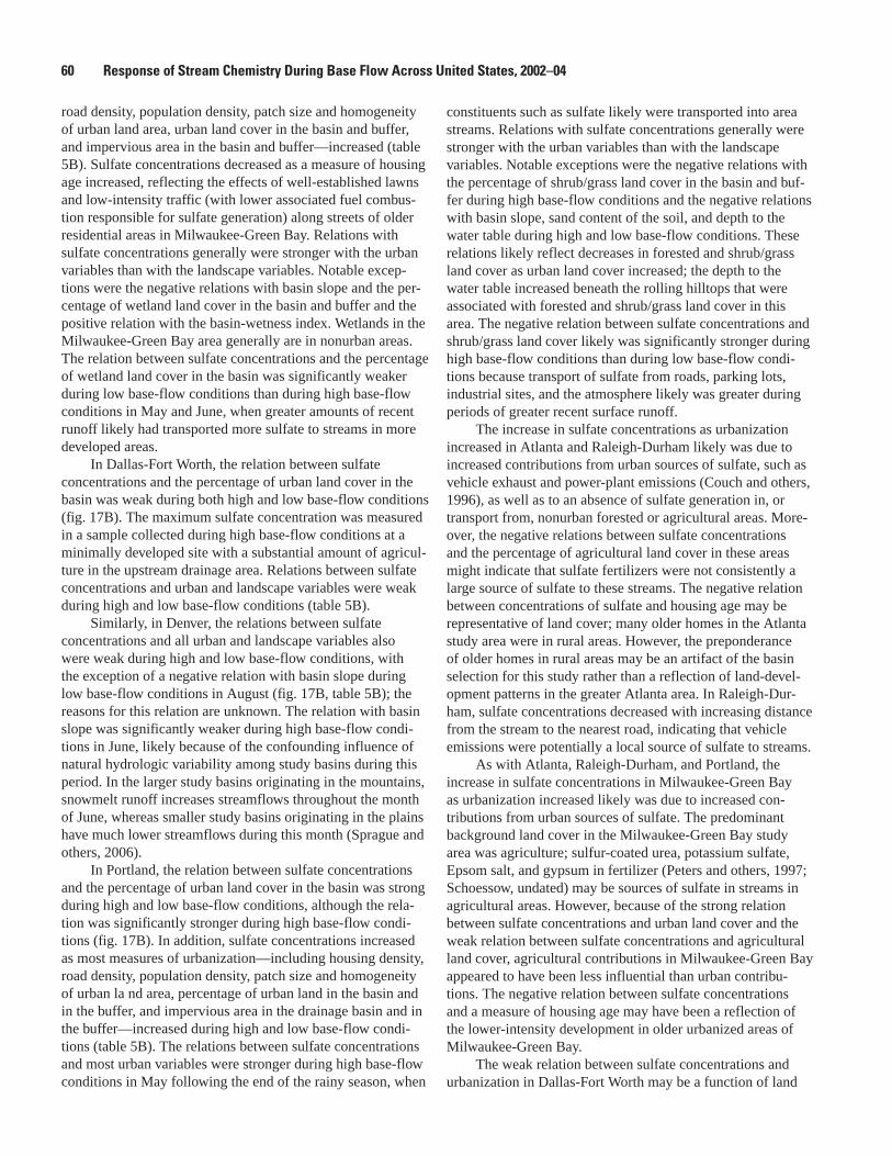
road density, population density, patch size and homogeneity of urban land area, urban land cover in the basin and buffer, and impervious area in the basin and buffer—increased (table 5B). Sulfate concentrations decreased as a measure of housing age increased, reflecting the effects of well-established lawns and low-intensity traffic (with lower associated fuel combus-tion responsible for sulfate generation) along streets of older residential areas in Milwaukee-Green Bay. Relations with sulfate concentrations generally were stronger with the urban variables than with the landscape variables. Notable excep-tions were the negative relations with basin slope and the per-centage of wetland land cover in the basin and buffer and the positive relation with the basin-wetness index. Wetlands in the Milwaukee-Green Bay area generally are in nonurban areas. The relation between sulfate concentrations and the percentage of wetland land cover in the basin was significantly weaker during low base-flow conditions than during high base-flow conditions in May and June, when greater amounts of recent runoff likely had transported more sulfate to streams in more developed areas.
In Dallas-Fort Worth, the relation between sulfate concentrations and the percentage of urban land cover in the basin was weak during both high and low base-flow conditions (fig. 17B). The maximum sulfate concentration was measured in a sample collected during high base-flow conditions at a minimally developed site with a substantial amount of agricul-ture in the upstream drainage area. Relations between sulfate concentrations and urban and landscape variables were weak during high and low base-flow conditions (table 5B).
Similarly, in Denver, the relations between sulfate concentrations and all urban and landscape variables also were weak during high and low base-flow conditions, with the exception of a negative relation with basin slope during low base-flow conditions in August (fig. 17B, table 5B); the reasons for this relation are unknown. The relation with basin slope was significantly weaker during high base-flow condi-tions in June, likely because of the confounding influence of natural hydrologic variability among study basins during this period. In the larger study basins originating in the mountains, snowmelt runoff increases streamflows throughout the month of June, whereas smaller study basins originating in the plains have much lower streamflows during this month (Sprague and others, 2006).
In Portland, the relation between sulfate concentrations and the percentage of urban land cover in the basin was strong during high and low base-flow conditions, although the rela-tion was significantly stronger during high base-flow condi-tions (fig. 17B). In addition, sulfate concentrations increased as most measures of urbanization—including housing density, road density, population density, patch size and homogeneity of urban la nd area, percentage of urban land in the basin and in the buffer, and impervious area in the drainage basin and in the buffer—increased during high and low base-flow condi-tions (table 5B). The relations between sulfate concentrations and most urban variables were stronger during high base-flow conditions in May following the end of the rainy season, when
constituents such as sulfate likely were transported into area streams. Relations with sulfate concentrations generally were stronger with the urban variables than with the landscape variables. Notable exceptions were the negative relations with the percentage of shrub/grass land cover in the basin and buf-fer during high base-flow conditions and the negative relations with basin slope, sand content of the soil, and depth to the water table during high and low base-flow conditions. These relations likely reflect decreases in forested and shrub/grass land cover as urban land cover increased; the depth to the water table increased beneath the rolling hilltops that were associated with forested and shrub/grass land cover in this area. The negative relation between sulfate concentrations and shrub/grass land cover likely was significantly stronger during high base-flow conditions than during low base-flow condi-tions because transport of sulfate from roads, parking lots, industrial sites, and the atmosphere likely was greater during periods of greater recent surface runoff.
The increase in sulfate concentrations as urbanization increased in Atlanta and Raleigh-Durham likely was due to increased contributions from urban sources of sulfate, such as vehicle exhaust and power-plant emissions (Couch and others, 1996), as well as to an absence of sulfate generation in, or transport from, nonurban forested or agricultural areas. More-over, the negative relations between sulfate concentrations and the percentage of agricultural land cover in these areas might indicate that sulfate fertilizers were not consistently a large source of sulfate to these streams. The negative relation between concentrations of sulfate and housing age may be representative of land cover; many older homes in the Atlanta study area were in rural areas. However, the preponderance of older homes in rural areas may be an artifact of the basin selection for this study rather than a reflection of land-devel-opment patterns in the greater Atlanta area. In Raleigh-Dur-ham, sulfate concentrations decreased with increasing distance from the stream to the nearest road, indicating that vehicle emissions were potentially a local source of sulfate to streams.
As with Atlanta, Raleigh-Durham, and Portland, the increase in sulfate concentrations in Milwaukee-Green Bay as urbanization increased likely was due to increased con-tributions from urban sources of sulfate. The predominant background land cover in the Milwaukee-Green Bay study area was agriculture; sulfur-coated urea, potassium sulfate, Epsom salt, and gypsum in fertilizer (Peters and others, 1997; Schoessow, undated) may be sources of sulfate in streams in agricultural areas. However, because of the strong relation between sulfate concentrations and urban land cover and the weak relation between sulfate concentrations and agricultural land cover, agricultural contributions in Milwaukee-Green Bay appeared to have been less influential than urban contribu-tions. The negative relation between sulfate concentrations and a measure of housing age may have been a reflection of the lower-intensity development in older urbanized areas of Milwaukee-Green Bay.
The weak relation between sulfate concentrations and urbanization in Dallas-Fort Worth may be a function of land
60 Response of Stream Chemistry During Base Flow Across United States, 2002–04

use and geology, and specifically, contributions of sulfate from the nonurban areas that obscure any contributions to sulfate concentrations from urban sources. The Woodbine aquifer underlies a substantial part of the Dallas-Fort Worth study area. Water from the Woodbine aquifer has sufficiently high concentrations of sulfate, iron, and manganese that the water is not potable and is instead used primarily for agricul-tural irrigation in the Dallas-Fort Worth study area (Reutter, 1996). Water samples collected in 1993 from 38 wells in the Woodbine aquifer had sulfate concentrations ranging from 19 to 3,400 mg/L, with a median concentration of 380 mg/L (Reutter, 1996). Other rural areas south of Dallas-Fort Worth are underlain by the Trinity aquifer and may have relatively high sulfate concentrations in base flow (Land and others, 1998). High sulfate concentrations in base flow in these rural areas may have obscured any pattern in sulfate concentrations relative to urban land cover in Dallas-Fort Worth. Likewise, in Denver, sulfate is the dominant anion in the alluvial ground water underlying parts of the study area (Bruce and McMahon, 1998). Therefore, natural sources likely obscured any pat-tern in sulfate concentrations relative to urban land cover in Denver.
The results for sulfate concentrations indicate that strate-gies to control sulfate transport to streams in urbanizing areas may be most effective when developed locally. In addition, in areas where sulfate concentrations in ground water are high, such strategies may need to consider the effects of ground-water inflow to streams.
Chloride
In Atlanta, the relation between chloride concentrations and the percentage of urban land cover in the basin was strong during high and low base-flow conditions (fig. 17C). Chloride concentrations increased as most measures of urbanization—including housing density, road density, population density, patch size and homogeneity of urban land area, percentage of urban land cover in the basin and buffer, and impervious area in the basin and buffer—increased (table 5C). There was a negative relation between chloride concentrations and a mea-sure of housing age, likely because many older homes in the Atlanta study area were in rural areas; however, this may have been an artifact of the basin selection for this study rather than a reflection of land-development patterns in the greater Atlanta area. There also was a negative relation between chloride con-centrations and distance from the stream to the nearest road, indicating that runoff from roads potentially was a local source of chloride to streams. This relation was significantly stronger during high base-flow conditions than during low base-flow conditions; transport of chloride from impervious areas such as roads and parking lots likely was greater during periods of recent surface runoff. Relations with chloride concentrations generally were stronger with the urban variables than with the landscape variables in Atlanta. The strongest relation with a landscape variable was a negative relation with the percent-
age of shrub/grass land cover in the basin, which may reflect changes in the background land cover.
In Raleigh-Durham, the relation between chloride con-centrations and the percentage of urban land cover in the basin was strong during high and low base-flow conditions (fig. 17C). Chloride concentrations increased as most measures of urbanization—including housing density, road density, popula-tion density, patch size and homogeneity of urban land area, percentage of urban land cover in the basin and buffer, and impervious area in the basin and buffer—increased (table 5C). Relations with chloride concentrations generally were stronger with the urban variables than with the landscape variables, with the exception of the negative relations with the percent-age of agriculture and shrub/grass land cover in the basin and buffer. These relations likely reflected the decrease in back-ground land cover as urban land cover increased.
In Milwaukee-Green Bay, the relation between chloride concentrations and the percentage of urban land cover in the basin was strong during high and low base-flow condi-tions (fig. 17C). Chloride concentrations increased as most measures of urbanization—including housing density, road density, population density, patch size and homogeneity of urban land area, urban land cover in the basin and buffer, and impervious area in the basin and buffer—increased (table 5C). The positive relations with urbanization may be attributable to increased residential use of water softeners, vehicle exhaust, or use of salt for pavement deicing in urban areas. In addition, chloride concentrations decreased as a measure of housing age increased, possibly because residential parts of mixed residen-tial/urban areas received less chloride from vehicle exhaust and deicing salt than did urban areas with freeway traffic and more extensive impervious areas such as parking lots. Rela-tions with chloride concentrations generally were stronger with the urban variables than with the landscape variables. The strongest relations with the landscape variables included negative relations with the percentage of agricultural and wet-land land cover in the basin and buffer and positive relations with the percentage of shrub/grass land cover in the basin and buffer. As with Atlanta and Raleigh-Durham, these relations likely reflected the increase in background land cover as urban land cover decreased.
In Dallas-Fort Worth, the relation between chloride con-centrations and the percentage of urban land cover in the basin was strong (fig. 17C), though the relations between chloride concentrations and some other urban and landscape variables were weak (table 5C). These results indicate that both urban and nonurban chloride sources likely were present. Both the Trinity and Woodbine aquifers that underlie parts of the Dal-las-Fort Worth study area have water with high concentrations of chloride (Land and others, 1998). High chloride concen-trations in base flow in these areas may have to some degree obscured increases in chloride concentrations as urbanization increased in Dallas-Fort Worth.
In Denver, the relation between chloride concentrations and the percentage of urban land cover in the basin was sig-nificantly stronger during low base-flow conditions in August
Response of Stream Chemistry to Gradients of Urbanization 61

than during high base-flow conditions in June (fig. 17C). Similarly, chloride concentrations were strongly related to road density, population density, patch size and homogeneity of urban land area, urban land cover in the basin, and impervi-ous area in the basin and negatively related to a measure of housing age during low base-flow conditions but not during high base-flow conditions (table 5C). The differences between high and low base-flow conditions likely were due to the confounding influence of natural hydrologic variability among study basins during high base-flow conditions—in the larger study basins originating in the mountains, snowmelt runoff increases streamflows throughout the month of June, whereas smaller study basins originating in the plains have much lower streamflows during this month (Sprague and others, 2006). Therefore, during this month, chloride concentrations might have been diluted by snowmelt runoff more in some basins than in others. In contrast, streamflows were uniformly low across all study basins during low base-flow conditions, and increases in chloride concentrations with urbanization poten-tially resulted from chloride in automobile exhaust, industrial emissions, and other urban sources. There also were negative relations between chloride concentrations and both housing age and the distance from the stream to the nearest road, possi-bly because older residential areas received less chloride from vehicle exhaust and runoff from roads was a local source of chloride to streams. In addition, chloride concentrations were negatively related to the percentage of agricultural land in the basin and in the buffer in Denver. Unlike in Atlanta, Raleigh-Durham, and Milwaukee-Green Bay, these relations do not reflect decreases in background land cover as urban land cover increased because increasing agricultural land cover was not proportional to decreasing urban land cover in Denver (fig. 2). Instead, this relation may reflect application of potassium chloride or increased salinity of irrigation return flow, or both, in agricultural areas.
In Portland, the relation between chloride concentrations and the percentage of urban land cover in the basin was strong (fig. 17C). Generally, chloride concentrations increased as many measures of urbanization—including housing density, road density, population density, urban land cover in the basin and buffer, and impervious area in the basin and buf-fer—increased (table 5C). These increases may be attributable to chloride in automobile exhaust, industrial emissions, and other urban sources. Relations with chloride concentrations generally were stronger with the urban variables than with the landscape variables in the Portland study area. However, chloride concentrations decreased with increasing percentages of shrub/grass land cover in the basin and buffer during high base-flow conditions and with increasing sand content in the soil and depth to the water table and decreasing soil erodibility during both high and low base-flow conditions. The relations with shrub/grass land cover and depth to water table likely reflected changes in the percentage of background land cover because shrub/grass land cover decreased as urban land cover increased and the mean depth to the water table increased beneath the rolling hilltops that were associated with back-
ground land cover in this area. The relation with shrub/grass land cover was significantly stronger during high base-flow conditions because transport of chloride from roads, parking lots, industrial sites, and the atmosphere likely was greater during periods of recent surface runoff. Areas with higher soil erodibility and lower permeability may have experienced increased surface runoff of chloride.
Chloride concentrations in Dallas-Fort Worth and Denver did not consistently increase with increasing urbanization. In contrast, chloride concentrations in Atlanta, Raleigh-Durham, Milwaukee-Green Bay, and Portland increased as urbaniza-tion increased, likely due in part to runoff of chloride-bearing salts applied to impervious areas for deicing (where used), wet and(or) dry deposition of chloride originating in vehicle exhaust, wet and dry deposition from industrial sources, and any discharge from WWTPs. The specific urban variables related to increasing chloride concentrations were the same among the four study areas, with the exception of housing age and distance from the stream to the nearest road. In Atlanta and Milwaukee-Green Bay, chloride concentrations decreased as a measure of housing age increased, reflecting the well-established lawns and low-intensity traffic in older residential areas in these two study areas. The specific landscape vari-ables related to increasing chloride concentrations differed between the four study areas, but most often the relations represented decreases in background land cover as urban land cover increased.
The results for chloride concentrations indicate that strategies to control chloride transport to streams in urbanizing areas may be most effective when developed locally. In addi-tion, in areas where chloride concentrations in ground water are high, such strategies may need to consider the effects of ground-water inflow to streams.
Comparison of the Patterns of Response to Urbanization Among Study Areas
The response of stream-water quality in base flow to urbanization differed by chemical constituent and by envi-ronmental setting. In areas where land cover in minimally urbanized basins was predominantly forest or shrub/grass, urbanization generally was associated with increasing chemi-cal concentrations, although other nonurban factors may have been related to chemical concentrations as well. In areas where minimally urbanized basins were already affected by other stressors, such as agriculture, water management, or inflow of relatively saline ground water, the effects of urbanization were less clear. Maintenance or protection of stream quality may be addressed by identifying all important stressors and supplementing the management practices currently used in urbanizing areas with additional steps to mitigate the effects of these other stressors.
62 Response of Stream Chemistry During Base Flow Across United States, 2002–04

Benchmark Exceedances
Available benchmarks for nutrients included human-health benchmarks for ammonia, nitrate, and nitrite; aquatic-life benchmarks for ammonia; and Ecoregional nutrient criteria for total nitrogen and total phosphorus (Appendix 3). SDWRs were available for pH, sulfate, and chloride, and aquatic-life benchmarks were available for pH and chloride (Appendix 3). Most of the 41 pesticides analyzed in this study had both human-health benchmarks (36 pesticides) and aquatic-life benchmarks (33 pesticides), but very few of the 24 pesticide degradates analyzed had benchmarks available (none for human health, and 3 for aquatic life) (Appendix 4). The type and number of benchmark exceedances for all constituents collectively is shown in figure 18 for each site in the six study areas. Appendix 5 lists the types of benchmarks exceeded and the constituents involved at each site.
Nutrients, pH, Sulfate, and Chloride
One or more Ecoregional nutrient criteria was exceeded at about 70 percent of sites. These exceedances did not appear to be related to the degree of urbanization in the basin, except that sites with less than about 3 percent urban land cover exceeded these baseline criteria less often (fig. 18). For the sites with less than 3 percent urban land cover, one or more Ecoregional criteria were exceeded in 38 percent of samples compared with 75 percent of samples for sites with more than 3 percent urban land cover, 81 percent for sites with more than 10 percent, and 83 percent for sites with more than 25 percent urban land cover. Ecoregional nutrient criteria are intended to indicate baseline conditions in rivers and streams—that is, conditions representing minimal effects from human activities.
Other nutrient benchmarks were rarely exceeded (fig. 18). The aquatic-life benchmark for ammonia was exceeded in samples from only 1 out of 173 sites—in both low and high base-flow samples from a Raleigh-Durham site with about 97 percent urban land use in the basin (Appendix 5). Human-health benchmarks for nutrients (specifically the MCL for nitrate) were exceeded in samples from 4 of 173 sites—at two sites each in Milwaukee-Green Bay and Dallas-Fort Worth. Two of these sites were in basins containing more than 25 per-cent urban land cover. Samples from the other two sites, both with less than 10 percent urban land cover, also exceeded the MCL for atrazine, which indicates there may be agricultural influences at these sites. It is important to emphasize that these exceedances occurred in ambient stream water rather than in finished drinking water. The comparison with human-health and drinking-water benchmarks does not permit evaluation of human exposure, but is part of a screening-level assessment to put the data in a human-health context.
For pH, sulfate, and chloride, aquatic-life benchmarks were exceeded in samples from 8 of 173 sites; all 8 sites were in either Atlanta, Raleigh-Durham, or Dallas-Fort Worth (fig. 18). The benchmark for pH was exceeded in seven samples
from seven sites in these study areas, and the benchmark for chloride was exceeded in 1 sample in Dallas-Fort Worth. One or more SDWRs for these constituents were exceeded in 31 samples from 24 sites in 5 study areas (all except Portland), indicating some possibility of taste and odor problems at these sites if the stream water were to be used as drinking water without treatment. Eleven of the 31 samples exceeded the SDWR for pH, 18 exceeded the SDWR for sulfate, and 1 sample exceeded the SDWR for chloride.
PesticidesOne or more human-health benchmarks for pesticide
compounds were exceeded in 16 samples from 13 sites in 3 study areas (Raleigh-Durham, Milwaukee-Green Bay, and Dallas-Fort Worth; Appendix 5), which was only about 3 percent of total samples from the 6 study areas (fig. 18). The pesticides with concentrations greater than human-health benchmarks were atrazine (8 samples), dieldrin (7 samples), and simazine (1 sample). There was no apparent relation with degree of urbanization, with exceedances occurring at sites ranging from 3 to 98 percent urban land cover. One exception was the dieldrin exceedances, which always occurred at sites with more than 60 percent urban land cover. As previously noted, the comparison of ambient stream-water concentra-tions with human-health benchmarks serves to put the data in a human-health context, but is not relevant to human exposure assessment.
Aquatic-life benchmarks were exceeded in only four samples from four sites in three study areas (Raleigh-Durham, Milwaukee-Green Bay, and Denver; Appendix 5), which was only about one percent of total samples from the six study areas (fig. 18). The sites with exceedances were in basins with 3 to 44 percent urban land cover. The pesticides that exceeded these benchmarks—malathion, chlorpyrifos, and diazinon—are all insecticides with known urban uses, although urban use of chlorpyrifos and diazinon probably declined prior to and during the study period because USEPA has phased out the residential uses of these insecticides by homeowners (U.S. Environmental Protection Agency, 2000a and 2005b)
Pesticide concentrations in streams show seasonality and other temporal variability, and these temporal patterns tend to differ regionally and locally. This variability results from differences in factors such as the timing and amounts of pesticide use, climate, and the frequency and magnitude of recent runoff from rainstorms or irrigation (Gilliom and others, 2006). Because this study sampled stream water only twice per year during base-flow conditions, it is likely that pesticide concentrations in these streams reached higher concentrations than those measured here. Therefore, the pesticide occurrence and benchmark exceedance rates described in this report may underestimate exceedances in ambient stream water at other times, such as in peak pesticide-use periods or during storms or irrigation return flow. In previous results from broader sampling as part of the USGS NAWQA Program (Gilliom and others, 2006), aquatic-life benchmarks were exceeded at over
Response of Stream Chemistry to Gradients of Urbanization 63

0
03.
23.
53.
74.
04.
45.
05.
05.
45.
55.
77.
411
.713
.814
.916
.317
.620
.224
.427
.330
.458
.862
.968
.978
.086
.087
.292
.897
.699
.110
0.0
0 0
3.0
3.1
4.4
5.2
6.0
7.3
12.4
20.0
20.7
23.7
38.8
39.3
55.9
60.1
65.7
66.8
72.2
76.1
76.4
79.0
82.1
92.6
94.2
96.8
96.9
96.9
98.4
100.
0
02.
32.
83.
63.
84.
54.
84.
95.
97.
311
.013
.416
.417
.820
.422
.122
.924
.825
.125
.735
.638
.339
.742
.643
.143
.260
.666
.267
.072
.585
.410
0.0 0
2.3
2.8
3.6
3.8
4.5
4.8
4.9
5.9
7.3
11.0
13.4
16.4
17.8
20.4
22.1
22.9
24.8
25.1
25.7
35.6
38.3
39.7
42.6
43.1
43.2
60.6
66.2
67.0
72.5
85.4
100.
0
3.0
3.1
4.4
5.2
6.0
7.3
12.4
20.0
20.7
23.7
38.8
39.3
55.9
60.1
65.7
66.8
72.2
76.1
76.4
79.0
82.1
92.6
94.2
96.8
96.9
96.9
98.4
100.
0
03.
23.
53.
74.
04.
45.
05.
05.
45.
55.
77.
411
.713
.814
.916
.317
.620
.224
.427
.330
.458
.862
.968
.978
.086
.087
.292
.897
.699
.110
0.0
2
4
6
8
0
2
4
6
8
0
2
4
6
8
0
2
4
6
8
0
2
4
6
8
0
2
4
6
8
EXPLANATIONCOLOR
Ecoregional nutrient criteria Nutrients
Pesticides
pH
Chloride or sulfate
Acute-invertebrate benchmark (Al)Acute water-quality criterion for the protection of aquatic organisms (Acute AWQC-AL)Chronic-invertebrate benchmark (Cl)
Chronic water-quality criterion for the protection of aquatic organisms (Chronic AWQC-AL)
Secondary drinking-water regulations (SDWR)Human-health benchmark (10-6 CRC, LHA, MCL)
PATTERN
PERCENTAGE OF URBAN LAND COVER IN BASIN
NUM
BER
OF B
ENCH
MAR
KS
EXCE
EDED
MILWAUKEE-GREEN BAY - HIGH BASE FLOW MILWAUKEE-GREEN BAY - LOW BASE FLOW
RALEIGH-DURHAM - HIGH BASE FLOW RALEIGH-DURHAM - LOW BASE FLOW
ATLANTA - HIGH BASE FLOW ATLANTA - LOW BASE FLOWN
UMBE
R OF
BEN
CHM
ARKS
EX
CEED
EDN
UMBE
R OF
BEN
CHM
ARKS
EX
CEED
ED
PERCENTAGE OF URBAN LAND COVER IN BASIN
Figure 18. The number and type of benchmark exceedances for all constituents combined in the Atlanta, Raleigh-Durham, Milwaukee-Green Bay, Dallas-Fort Worth, Denver, and Portland study areas. Each bar represents the sum of each type of exceedance in each basin. Not all types of benchmarks are available for all types of constituents. See Appendixes 3 and 4 for detailed information. Data are presented in Appendix 5. 10-6 CRC, U.S. Environmental Protection Agency 10-6 cancer risk concentration; LHA, U.S. Environmental Protection Agency lifetime health advisory; MCL, U.S. Environmental Protection Agency Maximum Contaminant Level.
64 Response of Stream Chemistry During Base Flow Across United States, 2002–04

00.
20.
40.
50.
61.
92.
33.
33.
54.
47.
17.
58.
613
.219
.022
.027
.128
.233
.037
.641
.959
.561
.972
.481
.082
.984
.388
.797
.810
0.0
01.
52.
84.
45.
88.
78.
710
.416
.617
.419
.220
.922
.225
.233
.338
.041
.449
.458
.959
.162
.663
.568
.872
.079
.688
.189
.390
.490
.410
0.0
01.
62.
32.
32.
52.
72.
83.
13.
34.
86.
56.
76.
97.
213
.915
.215
.317
.321
.361
.670
.271
.978
.983
.986
.010
0.0 0
2.3
2.3
2.5
2.5
2.7
2.8
3.3
4.8
6.5
6.7
6.9
7.2
9.4
13.9
15.2
15.3
17.3
21.3
70.2
71.9
78.9
83.9
86.0
88.8
100.
0
01.
52.
84.
45.
88.
78.
710
.416
.617
.419
.220
.922
.225
.233
.338
.041
.449
.458
.959
.162
.663
.568
.872
.079
.688
.189
.390
.490
.410
0.0
00.
20.
40.
50.
61.
92.
33.
33.
54.
47.
17.
58.
613
.219
.022
.027
.128
.233
.037
.641
.959
.561
.972
.481
.082
.984
.388
.797
.810
0.0
EXPLANATIONCOLOR
Ecoregional nutrient criteria NutrientsPesticidespHChloride or sulfate
Acute-invertebrate benchmark (Al)Acute water-quality criterion for the protection of aquatic organisms (Acute AWQC-AL)Chronic-invertebrate benchmark (Cl)
Chronic water-quality criterion for the protection of aquatic organisms (Chronic AWQC-AL)
Secondary drinking-water regulations (SDWR)Human-health benchmark (10-6 CRC, LHA, MCL)
PATTERN
PERCENTAGE OF URBAN LAND COVER IN BASIN
PORTLAND - HIGH BASE FLOW PORTLAND - LOW BASE FLOW
DENVER - HIGH BASE FLOW DENVER - LOW BASE FLOW
DALLAS-FORT WORTH - HIGH BASE FLOW DALLAS-FORT WORTH - LOW BASE FLOW
0
2
4
6
8
0
2
4
6
8
0
2
4
6
8N
UMBE
R OF
BEN
CHM
ARKS
EX
CEED
EDN
UMBE
R OF
BEN
CHM
ARKS
EX
CEED
EDN
UMBE
R OF
BEN
CHM
ARKS
EX
CEED
ED
PERCENTAGE OF URBAN LAND COVER IN BASIN
Figure 18. The number and type of benchmark exceedances for all constituents combined in the Atlanta, Raleigh-Durham, Milwaukee-Green Bay, Dallas-Fort Worth, Denver, and Portland study areas. Each bar represents the sum of each type of exceedance in each basin. Not all types of benchmarks are available for all types of constituents. See Appendixes 3 and 4 for detailed information. Data are presented in Appendix 5. 10-6 CRC, U.S. Environmental Protection Agency 10-6 cancer risk concentration; LHA, U.S. Environmental Protection Agency lifetime health advisory; MCL, U.S. Environmental Protection Agency Maximum Contaminant Level.—Continued
Response of Stream Chemistry to Gradients of Urbanization 65

80 percent of sites sampled in urban areas. On the other hand, because chronic aquatic-life benchmarks (intended for com-parison with 4- to 60-day average concentrations) were com-pared in this study with individual samples, exceedance rates described here may overestimate potential chronic toxicity.
SummaryDuring 2002–2004, the U.S. Geological Survey’s
National Water-Quality Assessment Program conducted a study to determine the effects of urbanization on stream ecosystems in six environmentally heterogeneous areas of the conterminous United States— Atlanta, Georgia; Raleigh-Durham, North Carolina; Milwaukee-Green Bay, Wisconsin; Dallas-Fort Worth, Texas; Denver, Colorado; and Portland, Oregon. This report describes the results from the stream chemistry component of the study. The objectives of this component were as follows: (1) to compare and contrast the response of stream chemistry during base flow to urbaniza-tion in different environmental settings; and (2) to examine the relation between the exceedance of water-quality benchmarks and the level of urbanization.
Within each metropolitan area, about 30 study basins were chosen to minimize natural variability between basins due to factors such as geology, altitude, and climate and to maximize coverage among basins of different degrees of urban development, ranging from minimally to highly developed. Water-quality samples were collected twice at each site, once during low base-flow conditions and once during high base-flow conditions. Chemical characteristics studied included concentrations of nutrients, dissolved pesticides and pesticide degradates, suspended sediment, sulfate, and chloride.
Nitrogen concentrations increased with urbanization in Atlanta, Raleigh-Durham, and Portland; relations between nitrogen concentrations and urbanization were weak in Milwaukee-Green Bay, Dallas-Fort Worth, and Denver. For-est was a predominant background land cover in basins with minimal urban development in Atlanta, Raleigh-Durham and Portland, and the increase in nitrogen concentrations fol-lowed the increase in urban land cover as forested land cover decreased in these areas. In contrast, nitrogen concentrations in basins with minimal urban development were consider-ably higher in Milwaukee-Green Bay and Dallas-Fort Worth, where agriculture was a predominant background land cover; agricultural influences may have obscured any increases in nitrogen concentrations related to urban development in these areas. Nitrogen concentrations in Denver were variable at all levels of urban development, which may have been due to the extensive water management in the study area.
There was a weak but positive relation between phos-phorus concentrations and urbanization in Atlanta, Raleigh-Durham, Dallas-Fort Worth, and Denver; the strongest positive relation was observed in Portland, where basins with minimal urban development had particularly low phosphorus concen-
trations. It is possible that leachate from septic tanks may have increased concentrations in basins with minimal urban devel-opment in Atlanta and Raleigh-Durham. In Milwaukee-Green Bay and Dallas-Fort Worth, phosphorus concentrations were high in basins with minimal urban development because of the high percentage of agricultural land cover in these basins. In Milwaukee-Green Bay, phosphorous concentrations decreased as urbanization increased and as agricultural land cover decreased, whereas in Dallas-Fort Worth, phosphorus con-centrations were similarly high in the most developed basins, leading to a weak overall relation between phosphorus and the degree of urbanization. Phosphorus concentrations in Denver were low overall relative to the other study areas and showed little distinct response to urbanization, which may have been due to the extensive water management in the study area.
The results for nutrient concentrations indicate that man-agement strategies to control nutrients in urbanizing areas may need to consider background, pre-development land cover. Particularly if development is occurring in agricultural areas, nutrient concentrations may be high even before development occurs.
Total herbicide concentrations increased with urbaniza-tion in Atlanta, Raleigh-Durham, and Portland, generally following the decrease in forested land cover and the increase in urban land cover. In Portland, there was evidence of mixed agricultural and urban influences at sites with 20 to 50 percent urban land cover; however, the overall relation between herbi-cide concentrations and urbanization was strong. In contrast, relations between total herbicide concentrations and urbaniza-tion were weak in Milwaukee-Green Bay, Dallas-Fort Worth, and Denver. In Milwaukee-Green Bay, where the background land cover was predominantly agriculture, total herbicide concentrations decreased somewhat as urbanization increased and as agricultural land cover decreased. In Dallas-Fort Worth, where agriculture and shrub/grass land cover were the pre-dominant background land covers, total herbicide concentra-tions were highest in basins with low urban and relatively high agricultural land cover, then decreased sharply as agricultural land cover decreased and shrub/grass land cover increased, and finally increased slightly again in the most urbanized basins. In Denver, where the predominant background land cover was shrub/grass land cover, total herbicide concentra-tions did not follow a clear pattern relative to any type of land cover, again possibly due to the extensive water management in the study area.
In Atlanta, Raleigh-Durham, and Portland, concentra-tions of total insecticides (like total herbicides) generally increased with increasing urbanization. In Milwaukee-Green Bay, Dallas-Fort Worth, and Denver, however, total insecticide concentrations were more strongly related to urbanization than were total herbicide concentrations. This relation may have been due to more intensive application of insecticides in urbanized basins, and—in Denver and Milwaukee-Green Bay—the fact that most study basins in these areas had a disproportionate amount of urban land cover in the lowland portion of the drainage area near the sampling sites, with much
66 Response of Stream Chemistry During Base Flow Across United States, 2002–04

of the herbicide loading originating further upstream. In Den-ver, the transport of urban insecticides to the nearby sampling sites may have been less affected by diversions and reservoir storage upstream than was the transport of herbicides from upstream agricultural areas.
Strategies to control herbicide transport to streams in urbanizing areas may be most effective when developed locally, and as with nutrients, such strategies may need to consider both agricultural and urban influences. Strategies to control insecticide transport to streams in urbanizing areas may be effective when developed nationally, although consid-eration of local factors likely will improve the outcome.
The pesticide signature for a given study area tended to show certain pesticides, and certain combinations of pesti-cides, as dominant, although the concentrations of the domi-nant pesticides varied markedly among sites within a study area. Normalization of pesticide concentrations in stream water by the pesticide toxicity index—an index of relative potential toxicity to cladocerans or fish—dramatically changed the pesticide signature, indicating that the pesticides with the greatest potential to adversely affect cladocerans or fish were not necessarily the pesticides detected at the highest concen-trations.
In all six study areas, the relation between suspended-sediment concentrations and urbanization was weak. In Atlanta, Raleigh-Durham, Milwaukee-Green Bay, and Port-land, there was an increase in sulfate and chloride concentra-tions with urbanization, likely due to increased contributions from urban sources of these constituents. In Dallas-Fort Worth and Denver, relations between sulfate concentrations and urbanization were weak. In Dallas-Fort Worth, the relation between chloride concentrations and the percentage of urban land cover in the basin was strong but the relations with other urban variables were weak; in Denver, the relation between chloride concentrations and urbanization was strong during low base-flow conditions but not during high base-flow condi-tions. These patterns in Dallas-Fort Worth and Denver likely were influenced in part by high sulfate and chloride concen-trations in ground-water inflow, which may have obscured increases in the concentrations with increasing urbanization.
The results for suspended-sediment concentrations sup-port previous research indicating that strategies to control sediment transport to streams in urbanizing areas may need to focus on conditions during stormwater runoff to a greater degree than conditions during base flow. The results for sulfate and chloride indicate that strategies to control their transport to streams in urbanizing areas may need to consider the effects of ground-water inflow to streams in areas where sulfate and chloride concentrations in alluvial ground water are high.
For nutrients, one or more recommended Ecoregional nutrient criteria were exceeded at about 70 percent of sites. These exceedances did not appear to be related to the degree of urbanization in the basin, except that sites with less than about three percent urban land cover less often exceeded these criteria, which represent baseline conditions for surface water that is minimally affected by human activities. Other nutrient
benchmarks were rarely exceeded. The aquatic-life benchmark for ammonia was exceeded at one site in Raleigh-Durham, and the human-health benchmark for nitrate was exceeded at four sites in Milwaukee-Green Bay and Dallas-Fort Worth.
For pH, sulfate, and chloride, aquatic-life benchmarks were exceeded at eight sites in three study areas (in Atlanta, Raleigh-Durham, and Dallas-Fort Worth). One or more sec-ondary drinking-water regulations were exceeded at 24 sites in 5 study areas (all except Portland), indicating some possibility of taste and odor problems at these sites if the stream water were to be used as drinking water without treatment.
For pesticides, one or more human-health benchmarks were exceeded by atrazine, dieldrin, or simazine at 13 sites in 3 study areas (Raleigh-Durham, Milwaukee-Green Bay, and Dallas-Fort Worth). There was no apparent relation with degree of urbanization, except that the dieldrin exceedances always occurred at sites with more than 60 percent urban land cover. Comparison of concentrations in individual ambient stream water samples with human-health benchmarks, which apply to lifetime consumption of drinking water, is not appro-priate for human exposure assessment but serves only to put the data in a human-health context. Aquatic-life benchmarks were exceeded at four sites in three study areas (Raleigh-Durham, Milwaukee-Green Bay, and Denver). There was no apparent relation with urban land cover, although the pesti-cides that exceeded the aquatic-life benchmarks—malathion, chlorpyrifos, and diazinon—are all insecticides with known urban uses.
Because this study sampled stream water only twice per year during base-flow conditions, it is likely that nutrient and pesticide concentrations in these streams reached higher con-centrations than those measured here. Therefore, the constitu-ent occurrence and benchmark exceedance rates described in this report may underestimate exceedances at other times, such as in peak pesticide and fertilizer use-periods or during storms or irrigation return flow. On the other hand, because chronic aquatic-life benchmarks (intended for comparison with 4- to 60-day average concentrations) were compared in this study with individual samples, exceedance rates described here may overestimate potential chronic toxicity.
In summary, the response of stream-water quality in base flow to urbanization differed by chemical constituent and by environmental setting. In areas where land cover in minimally urbanized basins was predominantly forest or shrub/grass, urbanization generally was associated with increasing chemi-cal concentrations, although other nonurban factors may have been related to chemical concentrations as well. In areas where minimally urbanized basins were already affected by other stressors, such as agriculture, water management, or inflow of relatively saline ground water, the effects of urbanization were less clear. Maintenance or protection of stream quality may be addressed by identifying all important stressors and supplementing the management practices currently used in urbanizing areas with additional steps to mitigate the effects of these other stressors.
Summary 67

References Cited
Bailey, H.C., Deanovic, Linda, Reyes, Emilie, Kimball, Tom, Larons, Karen, Cortright, Kristi, Connor, Valerie, and Hinton, D.E., 2000, Diazinon and chlorpyrifos in urban waterways in northern California, USA: Environmental Toxicology and Chemistry, v. 19, p. 82–87.
Black, R.W., Haggland, A.L., and Voss, F.D., 2000, Predicting the probability of detecting organochlorine pesticides and polychlorinated biphenyls in stream systems on the basis of land use in the Pacific Northwest, USA: Environmental Toxicology and Chemistry, v. 19, p. 1044–1054.
Booth, D.B., Hartley, David, and Jackson, Rhett, 2002, Forest cover, impervious-surface area, and the mitigation of storm-water impacts: Journal of the American Water Resources Association, v. 38, no. 3, p. 835–845.
Bruce, B.W., and McMahon, P.B., 1998, Shallow ground-water quality of selected land-use/aquifer settings in the South Platte River basin, Colorado and Nebraska 1993–95: U.S. Geological Survey Water-Resources Investigations Report 97–4229, 48 p.
Burton, G.A., Jr., and Pitt, R.E., 2002, Stormwater effects handbook: A toolbox for basin managers, scientists, and engineers: Boca Raton, Fla., Lewis Publishers, 911 p.
Church, P.E., and Friesz, P.J., 1993, Effectiveness of highway drainage systems in preventing road-salt contamination of groundwater—Preliminary findings: Transportation Research Board Transportation Research Record 1420, p. 56–64.
Couch, C.A., Hopkins, E.H., and Hardy, P.S., 1996, Influ-ences of environmental settings on aquatic ecosystems in the Apalachicola-Chattahoochee-Flint River basin: U.S. Geological Survey Water-Resources Investigations Report 95–4278, 58 p.
Crawford, C.G., 2001, Factors affecting pesticide occurrence and transport in a large midwestern river basin: Journal of the American Water Resources Association, v. 37, p. 1–16.
Cuffney, T.F., Zappia, Humbert, Giddings, E.M.P., and Coles, J.F., 2005, Effects of urbanization on benthic macroinver-tebrate assemblages in contrasting environmental set-tings—Boston, Massachusetts; Birmingham, Alabama; and Salt Lake City, Utah, in Brown, L.R., Gray, R.H., Hughes, R.M., and Meador, M.R., eds., Effects of urbanization on stream ecosystems: Bethesda, Maryland, American Fisher-ies Society, Symposium 47, p. 361–407.
Daymet, 2005, Daily surface weather data and climatological summaries: Numerical Terradynamic Simulation Group, University of Montana, accessed December 1, 2005, at http://www.daymet.org.
Environment Canada, 2001, Summary of the report of the assessment of the substance road salts specified on the pri-ority substances list: Canada Gazette Part 1, v. 135, no. 48, p. 4335–4340.
Everitt, B. S., Landau, Sabine, and Leese, Morven, 2001, Cluster analysis, 4th edition: London, Arnold Publishers, 237 p.
Falcone, J.A., Stewart, J.S., Sobieszczyk, Steven, Dupree, J.A., McMahon, Gerard, and, Buell, G.R., 2007, A comparison of natural and urban characteristics and the development of urban intensity indices across six geographic settings: U.S. Geological Survey Scientific Investigations Report 2007–5123, 133 p.
Fisher, R.A., 1921, On the ‘probable error’ of a coefficient of correlation deduced from a small sample: Metron, v. I, p. 3–32
Fishman, M.J., 1993, Methods of analysis by the U.S. Geo-logical Survey National Water-Quality Laboratory—Deter-mination of inorganic and organic constituents in water and fluvial sediments: U.S. Geological Survey Open-File Report 93–125, 217 p.
Fuhrer, G.J., Gilliom, R.J., Hamilton, P.A., Morace, J.L., Nowell, L.H., Rinella, J.F., Stoner, J.D., and Wentz, D.A., 1999, The quality of our Nation’s waters—Nutrients and pesticides: U.S. Geological Survey Circular 1225, 82 p.
GeoLytics, 2001, CensusCD 2000 and StreetCD 2000: Geo-Lytics, Inc., East Brunswick, New Jersey, CD-ROM.
Gilliom, R.J., 2001, Pesticides in the hydrologic system—What do we know and what’s next?: Hydrologic Processes, v. 15, p. 3197–3201.
Gilliom, R.J., Barbash, J.E., Crawford, C.G., Hamilton, P.A., Martin, J.D., Nakagaki, Naomi, Nowell, L.H., Scott, J.C., Stackelberg, P.E., Thelin, G.P., and Wolock, D.M., 2006, The quality of our Nation’s water—Pesticides in the Nation’s streams and ground water, 1992–2001: U.S. Geological Survey Circular 1291, 169 p.
Goldman, S.J., Jackson, Katharine, and Bursztynsky, T.A., 1986, Erosion and sediment control handbook: New York, McGraw-Hill, 443 p.
Graffy, E.A., Helsel, D.R., and Mueller, D.K., 1996, Nutrients in the Nation’s waters—Identifying problems and progress: U.S. Geological Survey Fact Sheet FS–218–96, 6 p.
Grove, J.M., and Burch, W.R., 1997, A social ecology approach and applications of urban ecosystem and land-scape analyses—A case study of Baltimore, Maryland: Urban Ecosystems, v. 1, p. 259–275.
68 Response of Stream Chemistry During Base Flow Across United States, 2002–04
Guy, H.P., 1969, Laboratory theory and methods for sediment analysis: U.S. Geological Survey Techniques of Water-Resources Investigations, book 5, chap. C1, 58 p.
Haith, D.A., 1976, Land use and water quality in New York rivers: Journal of the Environmental Engineering Division, American Society of Civil Engineers, v. 102, no. EE1, Proceedings Paper 11902, p. 1–15.
Heany, J.P., and Huber, W.C., 1984, Nationwide assessment of urban runoff impact on receiving water quality: Water Resources Bulletin, v. 20, p. 35–42.
Heisig, P.M., 2000, Effects of residential and agricultural land uses on the chemical quality of base flow of small streams in the Croton basin, southeastern New York: U.S. Geologi-cal Survey Water-Resources Investigations Report 99–4173, 15 p.
Helsel, D.R., and Hirsch, R.M., 1992, Statistical methods in water resources: Amsterdam, Elsevier, 529 p.
Hem, J.D., 1985, Study and interpretation of the chemical characteristics of natural water: U.S. Geological Survey Water-Supply Paper 2254, 272 p.
Herlihy, A.T., Stoddard, J.L., and Johnson, C.B., 1998, The relationship between stream chemistry and basin land cover data in the Mid-Atlantic Region: U.S. Water, Air, and Soil Pollution, v. 105, p. 377–386
Hoffman, R.S., Capel, P.D., and Larson, S.J., 2000, Compari-son of pesticides in eight U.S. urban streams: Environmen-tal Toxicology and Chemistry, v. 19, p. 2249–2258.
Hogg, R.V., and Tanis, E.A., 1993, Probability and statisti-cal inference (4th ed.): New York, Macmillan Publishing Company, 731 p.
House, M.A., Ellis, J.B., Herricks, E.E., Hvitved-Jacobsen, T., Seager, J., Lijklema, L., Aaldernik, H., and Clifforde, I.T., 1993, Urban drainage—Impacts on receiving water quality: Water Science and Technology, v. 27, p. 117–158.
Johnson, C.D., and Juengst, Dotty, 1997, Polluted urban run-off—A source of concern: University of Wisconsin-Exten-sion Report I–02–97–5M–20–S, 4 p.
Kaushal, S.S., Groffman, P.M., Likens, G.E., Belt, K.T., Stack, W.P., Kelly, V.R., Band, L.E., and Fisher, G.T., 2005, Increased salinization of fresh water in the northeastern United States: Proceedings of the National Academy of Sciences, v. 102, p. 13517–13520.
Kiely, Timothy, Donaldson, David, and Grube, Arthur, 2004, Pesticides industry sales and usage—2000 and 2001 market estimates: U.S. Environmental Protection Agency Report EPA–733–R–04–001, 48 p.
Klein, R.D., 1979, Urbanization and stream quality impair-ment: Water Resources Bulletin, v. 15, no. 4, p. 948–963.
Krug, W.R., and Goddard, G.L., 1986, Effects of urbanization on stream flow, sediment loads, and channel morphology in Pheasant Branch basin near Middleton, Wisconsin: U.S. Geological Survey Water-Resources Investigations Report 85–4068, 82 p.
Kunze, A.E., and Sroka, B.N., 2004, Effects of highway deicing chemicals on shallow unconsolidated aquifers in Ohio—Final report: U.S. Geological Survey Scientific Investigations Report 2004–5150, 199 p.
Land, L.F., Moring, J.B., Van Metre, P.C., Reutter, D.C., Mahler, B.J., Shipp, A.A., and Ulery, R.L., 1998, Water quality in the Trinity River basin, Texas, 1992–95: U.S. Geological Survey Circular 1171, 39 p.
Landers, M.N., Ankcorn, P.D., McFadden, K.W., and Gregory, M.B., 2002, Does land use affect our streams? A watershed example from Gwinnett County, Georgia, 1998–2001: U.S. Geological Survey Water-Resources Investigations Report 02–4281, 6 p.
Lough, G.C., Schauer, J.J., Park, June-Soo, Shafer, M.M., Deminter, J.T., and Weinstein, J.P., 2005, Emissions of met-als associated with motor vehicle roadways: Environmental Science and Technology, v. 39, p. 826–836.
Maltby, Lorraine, Blake, Naomi, Brock, T.C.M., and Van Den Brink, P.J., 2005, Insecticide species sensitivity distribu-tions: Importance of test species selection and relevance to aquatic ecosystems: Environmental Toxicology and Chem-istry, v. 24, no. 2, p. 379–388.
McGarigal, Kevin, Cushman, S.A., Neel, M.C., and Ene, Edu-ard, 2002, FRAGSTATS: Spatial pattern analysis program for categorical maps, FRAGSTATS 3.1, University of Mas-sachusetts, Amherst, accessed July 1, 2005, at http://www.umass.edu/landeco/research/fragstats/fragstats.html.
McMahon, Gerard, and Cuffney, T.F., 2000, Quantifying urban intensity in drainage basins for assessing stream ecologi-cal conditions: Journal of the American Water Resources Association, v. 36, p. 1247–1261.
McKnight, T.L., 2001, Regional geography of the United States and Canada: Prentice Hall, Upper Saddle River, New Jersey, 525 p.
Meador, M.R., Coles, J.F., and Zappia, Humbert, 2005, Fish assemblage responses to urban intensity gradients in contrasting metropolitan areas: Birmingham, Alabama, and Boston, Massachusetts, in Brown, L.R., Gray, R.H., Hughes, R.M., and Meador, M.R., eds., Effects of urbaniza-tion on stream ecosystems: American Fisheries Society, Symposium 47, Bethesda, Maryland, p. 409–423.
References Cited 69

Meng, X.L., Rosenthal, Robert, and Rubin, D.B., 1992, Com-paring correlated correlation coefficients: Psychological Bulletin, v. 111, p. 172–175.
Meyer, J.L., Paul, M.J., and Taulbee, W.K., 2005, Stream ecosystem function in urbanizing landscapes: Journal of the North American Benthological Society, v. 24, no. 3, p. 602–612.
Miller, T.L., and Hamilton, P.A., 2001, Selected findings and current perspectives on urban and agricultural water quality by the National Water-Quality Assessment Program: U.S. Geological Survey Fact Sheet FS–047–01, 2 p.
Mueller, D.K., Hamilton, P.A., Helsel, D.R., Hitt, K.J., and Ruddy, B.C., 1995, Nutrients in ground water and surface water of the United States—An analysis of data through 1992: U.S. Geological Survey Water-Resources Investiga- tions Report 95–4031, 74 p.
Mueller, D.K., and Helsel, D.R., 1996, Nutrients in the Nation’s waters—Too much of a good thing?: U.S. Geologi-cal Survey Circular 1136, 24 p.
Mueller, D.K., Martin, J.D., and Lopes, T.J., 1997, Quality-control design for surface-water sampling in the National Water-Quality Assessment Program: U.S. Geological Survey Open-File Report 97–223, 17 p.
Munn, M.D., and Gilliom, R.J., 2001, Pesticide toxicity index for freshwater aquatic organisms: U.S. Geological Survey Water-Resources Investigations Report 01–4077, 55 p.
Munn, M.D., Gilliom, R.J., Moran, P.W., and Nowell, L.H., 2006, Pesticide toxicity index for freshwater aquatic organ-isms (2nd ed.): U.S. Geological Survey Scientific Investiga-tions Report 2006–5148, 81 p.
National Oceanic and Atmospheric Administration, 2005, Coastal change analysis program: National Oceanic and Atmospheric Administration on-line database, accessed December 1, 2005, at http://www.csc.noaa.gov/crs/lca/ccap.html.
Omernik, J.M., 1987, Ecoregions of the conterminous United States: Annals of the Association of American Geographers, v. 77, p. 118–125.
Parker J.T., Fossum, K.D., Ingersoll, T.L., 2000, Chemical characteristics of urban stormwater sediments and implica-tions for environmental management, Maricopa County, Arizona: Environmental Management, v. 26, p. 99–115.
Parkhurst, D.F., 2001, Statistical significance tests—Equiva-lence and reverse tests should reduce misinterpretation: Bioscience, v. 51, p. 1051–1057.
Paul, M.J., and Meyer, J.L., 2001, Streams in the urban land-scape: Annual Review of Ecology and Systematics, v. 32, p. 333–365.
Pereira, W.E., Domagalski, J.L., Hostettler, F.D., Brown, L.R., and Rapp, J.B., 1996, Occurrence and accumulation of pesticides and organic contaminants in river sediment, water and clam tissues from the San Joaquin River and tributaries, California: Environmental Toxicology and Chemistry, v. 15, p. 172–180.
Peters, C.A., Robertson, D.M., Saad, D.A., Sullivan, D.J., Scudder, B.C., Fitzpatrick, F.A., Richards, K.D., Stewart, J.S., Fitzgerald, S.A., Lenz, B.N., 1997, Water quality in the western Lake Michigan drainages, Wisconsin and Michigan, 1992–95, U.S. Geological Survey Circular 1156, 40 p.
Phillips P.J., and Bode, R.W., 2004, Pesticides in surface water runoff in south-eastern New York State, USA—Seasonal and stormflow effects on concentrations: Pest Management Science, v. 60, p. 531–543.
Pitt, R.E., Field, R., Lalor, M., and Brown, M., 1995, Urban stormwater toxic pollutants—Assessment, sources, and treatability: Water Environment Research, v. 67, p. 260–275.
Potapova, Marina, Coles, J. F., Giddings, E.M., and Zappia, Humbert, 2005, A comparison of the influences of urban-ization on stream benthic algal assemblages in contrasting environmental settings, in Brown, L.R., Gray, R.H., Hughes, R.M., and Meador, M.R., eds., Effects of urbanization on stream ecosystems: American Fisheries Society, Sympo-sium 47, Bethesda, Maryland, p. 333–359.
Reutter, D.C., 1996, National water-quality assessment of the Trinity River basin, Texas—Well and water-quality data from the outcrop of Woodbine Aquifer in urban Tarrant County, 1993: U.S. Geological Survey Open-File Report 96–413, 32 p.
Roy, A.H., Rosemond, A.D., Paul, M.J., Leigh, D.S., and Wallace, J.B., 2003, Stream macroinvertebrate response to catchment urbanization (Georgia, U.S.A.): Freshwater Biology, v. 48, p. 329–346.
Santa Clarita Valley Joint Sewerage System, 2002, Chloride source report: Santa Clarita Valley Sanitation District, Los Angeles County, California, accessed October 1, 2006, at http://lifesourcewater.com/pdfs/Chloride_Report.pdf.
Schoessow, Kevin, undated, Manufactured vs. natural fertil-izers, University of Wisconsin Agricultural Extension Fact Sheet, 2 p.
Schoonover, J.E., Lockaby, B.G., and Pan, Shufen, 2005, Changes in chemical and physical properties of stream water across an urban-rural gradient in western Georgia: Urban Ecosystems, v. 8, no. 1, p. 107–124.
70 Response of Stream Chemistry During Base Flow Across United States, 2002–04
Seitzinger, S.P., Harrison J.A., Bohlke, J.K., Bouwman, A.F., Lowrance, R., Peterson, B., Tobias, C., and Van Drecht, G., 2006, Denitrification across landscapes and waterscapes—A synthesis: Ecological Applications, v. 16, no. 6, p. 2064–2090.
Short, T.M., Giddings, E.M.P., Zappia, Humbert, and Coles, J.F., 2005, Urbanization effects on habitat characteristics of streams in Boston, Massachusetts, Birmingham, Ala-bama, and Salt Lake City, Utah, in Brown, L.R., Gray, R.H., Hughes, R.M., and Meador, M.R., eds., Effects of urbaniza-tion on stream ecosystems: American Fisheries Society, Symposium 47, Bethesda, Maryland, p. 317–332.
Sprague, L.A., Langland, M.J., Yochum, S.E., Edwards, R.E., Blomquist, J.D., Phillips, S.W., Shenk, G.W., and Preston, S.D., 2000, Factors affecting nutrient trends in major rivers of the Chesapeake Bay watershed: U.S. Geological Survey Water-Resources Investigations Report 2000–4218, 109 p.
Sprague, L.A., Zuellig, R.E., and Dupree, J.A., 2006, Effects of urbanization on stream ecosystems in the South Platte River basin, Colorado and Wyoming, chap. A of Effects of urbanization on stream ecosystems in six metropolitan areas of the United States: U.S. Geological Survey Scientific Investigations Report 2006–5101–A, 139 p.
Stone, Michael, and Droppo, I.G., 1994, In-channel surficial fine-grained sediment laminae (Part II)—Chemical char-acteristics and implications for contaminant transport by fluvial sediments: Hydrological Processes, v. 8, p.113–124.
Tate, C.M., and Heiny, J.S., 1996, Organochlorine compounds in bed sediment and fish tissue in the South Platte River basin, USA, 1992–1993: Archives of Environmental Con-tamination and Toxicology, v. 30, p. 62–78.
Tate, C.M., Cuffney, T.F., McMahon, Gerard, Giddings, E.M.P., and Zappia, Humbert, 2005, Use of an urban inten-sity index to assess urban effects on streams in three con-trasting environmental settings, in Brown, L.R., Gray, R.H., Hughes, R.M., and Meador, M.R., eds., Effects of urbaniza-tion on stream ecosystems: American Fisheries Society, Symposium 47, Bethesda, Maryland, p. 291–315.
Toccalino, P.L., Nowell, L.H., Wilber, W.G., Zogorski, J.S., Donohue, J.M., Eiden, C.A., Krietzman, S.J., and Post, G.B., 2003, Development of health-based screening levels for use in state- or local-scale water-quality assessments: U.S. Geological Survey Water-Resources Investigations Report 03–4054, 22 p.
Toccalino, P.L., Rowe, B.L., and Norman, J.E., 2006, Volatile organic compounds in the Nation’s drinking-water supply wells—What findings may mean to human health: U.S. Geological Survey Fact Sheet 2006–3043, 4 p.
Trimble, S.W., 1974, Man-induced soil erosion on the South-ern Piedmont, 1700–1970: Soil Conservation Society of America, Ankeny, Iowa.
Trimble, S.W., 1997, Contribution of stream channel erosion to sediment yield from an urbanizing basin: Science, v. 278, p. 1442–1444.
U.S. Army Corps of Engineers, 1996, Water control infrastruc-ture, national inventory of dams, 1995–1996: U.S. Federal Emergency Management Agency, Arlington, Virginia, CD-ROM.
U.S. Department of Agriculture, 1994, State soil geographic (STATSGO) data base: U.S. Department of Agriculture Natural Resources Conservation Service Miscellaneous Publications 1492, 110 p. and computer data.
U.S. Environmental Protection Agency, 1992, Water quality standards; Establishment of numeric criteria for priority toxic pollutants; States’ compliance; Final rule (12/22/092) (“Toxics Rule”): Federal Register, v. 57, no. 246, p. 60848–60923.
U.S. Environmental Protection Agency, 1994a, Reregistration eligibility decision for pronamide, list A, case 0082: U.S. Environmental Protection Agency, accessed October 31, 2005, at http://www.epa.gov/oppsrrd1/REDs/old_reds/pron-amide.pdf.
U.S. Environmental Protection Agency, 1994b, Reregistration eligibility decision (RED) hexazinone: U.S. Environmental Protection Agency, Office of Prevention, Pesticides and Toxic Substances, EPA 738–R–94–022, September 1994, accessed March 14, 2006, at http://www.epa.gov/oppsrrd1/REDs/0266.pdf.
U.S. Environmental Protection Agency, 1994c, Reregistration eligibility decision (RED) metalaxyl: U.S. Environmental Protection Agency, Office of Prevention, Pesticides and Toxic Substances, EPA 738–R–94–017, September 1994, accessed March 17, 2006, at http://www.epa.gov/oppsrrd1/REDs/0081.pdf.
U.S. Environmental Protection Agency, 1994d, Reregistra-tion eligibility decision, tebuthiuron, list A, case 0054: U.S. Environmental Protection Agency, Office of Pesticide Programs, Special Review and Reregistration Division, accessed September 20, 2005, at http://www.epa.gov/oppsrrd1/REDs/old_reds/tebuthiuron.pdf.
U.S. Environmental Protection Agency, 1995a, Reregistration eligibility decision (RED) metolachlor: U.S. Environmental Protection Agency, Prevention, Pesticides and Toxic Sub-stances, EPA 738–R–95–006, April 1995, accessed Septem-ber 22, 2005, at http://www.epa.gov/oppsrrd1/REDs/0001.pdf.
References Cited 71

U.S. Environmental Protection Agency, 1995b, Reregistra-tion eligibility decision (RED) terbuthylazine: U.S. Envi-ronmental Protection Agency, Prevention, Pesticides and Toxic Substances, EPA 738–R–95–005, March 1995, accessed March 17, 2006, at http://www.epa.gov/oppsrrd1/REDs/2645.pdf.
U.S. Environmental Protection Agency, 1996a, Reregistration eligibility decision (RED) prometryn: U.S. Environmental Protection Agency, Office of Prevention, Pesticides and Toxic Substances, EPA 738–R–95–033, February 1996, accessed March 17, 2006, at http://www.epa.gov/oppsrrd1/REDs/0467.pdf.
U.S. Environmental Protection Agency, 1996b, Reregistration eligibility decision (RED) trifluralin: U.S. Environmental Protection Agency, Office of Pesticide Programs, Special Review and Reregistration Division, EPA 738–R–95–040, accessed September 14, 2005, at http://www.epa.gov/oppsrrd1/REDs/0179.pdf.
U.S. Environmental Protection Agency, 1997, Reregistration eligibility decision (RED) pendimethalin: U.S. Environ-mental Protection Agency, Prevention, Pesticides and Toxic Substances, EPA 738–R–97–007, June 1997, accessed October 5, 2005, at http://www.epa.gov/oppsrrd1/REDs/0187red.pdf.
U.S. Environmental Protection Agency, 1998a, EFED RED chapter for isofenphos (Environmental fate and effects preliminary assessment): U.S. Environmental Protection Agency, Office of Prevention, Pesticides and Toxic Sub-stances, Environmental Fate and Effects Division, accessed March 14, 2006, at http://www.epa.gov/pesticides/op/isofen-phos/isoefed.pdf.
U.S. Environmental Protection Agency, 1998b, Environmen-tal Fate and Effects Division RED chapter for phosmet (Revised environmental fate and effects risk assessment): U.S. Environmental Protection Agency, Office of Preven-tion, Pesticides and Toxic Substances, Environmental Fate and Effects Division, April 1998, accessed March 17, 2006, at http://www.epa.gov/pesticides/op/phosmet/efedrra.pdf.
U.S. Environmental Protection Agency, 1998c, Preliminary environmental fate and effects assessment, EFED science chapter for phorate RED August 7, 1998: U.S. Environ-mental Protection Agency, Environmental Fate and Effects Division, accessed October 4, 2005, at http://www.epa.gov/pesticides/op/phorate/phorefed.pdf.
U.S. Environmental Protection Agency, 1998d, Reregistra-tion eligibility decision (RED) alachlor: U.S. Environmen-tal Protection Agency, Prevention, Pesticides and Toxic Substances, EPA 738–R–98–020, December 1998, accessed September 14, 2005, at http://www.epa.gov/oppsrrd1/REDs/0063.pdf.
U.S. Environmental Protection Agency, 1998e, Reregistra-tion eligibility decision (RED) DCPA: U.S. Environmen-tal Protection Agency, Prevention, Pesticides and Toxic Substances, EPA 738–R–98–005, November 1998, accessed September 21, 2005, at http://www.epa.gov/oppsrrd1/REDs/0270red.pdf.
U.S. Environmental Protection Agency, 1998f, Reregistration eligibility decision (RED) iprodione: U.S. Environmental Protection Agency, Office of Prevention, Pesticides and Toxic Substances, EPA 738–R–98–019, November 1994, accessed March 14, 2006, at http://www.epa.gov/oppsrrd1/REDs/2335.pdf.
U.S. Environmental Protection Agency, 1998g, Reregistration eligibility decision (RED) metribuzin: U.S. Environmen-tal Protection Agency, Prevention, Pesticides and Toxic Substances, EPA 738–R–97–006. February 1998, accessed September 15, 2005, at http://www.epa.gov/oppsrrd1/REDs/0181red.pdf.
U.S. Environmental Protection Agency, 1998h, Transmittal of EFED List, A summary report for ethion (Environmental fate and effects preliminary assessment): U.S. Environmen-tal Protection Agency, Prevention, Pesticides and Toxic Substances, accessed March 14, 2006, at http://www.epa.gov/pesticides/op/ethion/ethiefed.pdf.
U.S. Environmental Protection Agency, 1999a, EFED RED chapter for dicrotophos: U.S. Environmental Protec-tion Agency, Office of Prevention, Pesticides and Toxic Substances, accessed March 13, 2006, at http://www.epa.gov/oppsrrd1/op/dicrotophos/efed-dicro.pdf.
U.S. Environmental Protection Agency, 1999b, Revised envi-ronmental fate and effects assessment, outline of section C, Environmental assessment [phorate] September 14, 1999: U.S. Environmental Protection Agency, accessed October 4, 2005, at http://www.epa.gov/pesticides/op/phorate/phora-teefedrevrisk2of6.pdf.
U.S. Environmental Protection Agency, 1999c, Revised envi-ronmental fate and effects assessment [terbufos], section 4, Ecological toxicity data: U.S. Environmental Protection Agency, September 14, 1999, accessed October 4, 2005, at http://www.epa.gov/oppsrrd1/op/terbufos/efed_toxdata.pdf.
U.S. Environmental Protection Agency, 2000a, Chlorpyrifos revised risk assessment and agreement with registrants: U.S. Environmental Protection Agency Fact Sheet, accessed September 21, 2005, at http://www.epa.gov/oppsrrd1/op/chlorpyrifos/presentation.pdf.
U.S. Environmental Protection Agency, 2000b, EFED risk assessment for reregistration eligibility science chapter for chlorpyrifos, fate and environmental risk assessment chapter: U.S. Environmental Protection Agency June 2000, accessed September 21, 2005, at http://www.epa.gov/oppsrrd1/op/chlorpyrifos/efedrra1.pdf.
72 Response of Stream Chemistry During Base Flow Across United States, 2002–04

U.S. Environmental Protection Agency, 2000c, Environmental risk assessment for diazinon: U.S. Environmental Protection Agency, accessed September 21, 2005, at http://www.epa.gov/pesticides/op/diazinon/risk_oct2000.pdf.
U.S. Environmental Protection Agency, 2000d, Malathion reregistration eligibility document, environmental fate and effects chapter, revised November 9, 2000: U.S. Environ-mental Protection Agency, accessed September 22, 2005, at http://www.epa.gov/oppsrrd1/op/malathion/efedrra.pdf.
U.S. Environmental Protection Agency, 2000e, The quality of our Nation’s waters: U.S. Environmental Protection Agency, EPA 841–S–00–001, 20 p.
U.S. Environmental Protection Agency, 2001, Fenamiphos environmental risk assessment: U.S. Environmental Protec-tion Agency, Prevention, Pesticides and Toxic Substances, Environmental fate and Effects Division, accessed March 14, 2006, at http://www.epa.gov/oppsrrd1/op/fenamiphos/env_risk.pdf.
U.S. Environmental Protection Agency, 2002a, Ecoregional nutrient criteria: U.S. Environmental Protection Agency Fact Sheet EPA-822-F-02-00, October 2002, accessed April 18, 2006, at http://www.epa.gov/waterscience/criteria/nutri-ent/ecoregions/jan03frnfs.pdf.
U.S. Environmental Protection Agency, 2002b, Interim rereg-istration eligibility decision for chlorpyrifos: U.S. Environ-mental Protection Agency, Prevention, Pesticides and Toxic Substances, EPA 738–R–01–007, February 2002, accessed September 21, 2005, at http://www.epa.gov/oppsrrd1/REDs/chlorpyrifos_ired.pdf.
U.S. Environmental Protection Agency, 2002c, Interim rereg-istration eligibility decision for dicrotophos: U.S. Environ-mental Protection Agency, Office of Prevention, Pesticides and Toxic Substances, accessed March 13, 2006, at http://www.epa.gov/oppsrrd1/REDs/dicrotophos_ired.pdf.
U.S. Environmental Protection Agency, 2002d, Interim rereg-istration eligibility decision for fenamiphos: U.S. Environ-mental Protection Agency, Prevention, Pesticides and Toxic Substances, EPA 738–R–02–004, May 2002, accessed March 14, 2006, at http://www.epa.gov/oppsrrd1/REDs/fenamiphos_ired.pdf.
U.S. Environmental Protection Agency, 2002e, Interim rereg-istration eligibility decision for methidathion: U.S. Envi-ronmental Protection Agency, Prevention, Pesticides and Toxic Substances, April 2002, accessed March 17, 2006, at http://www.epa.gov/oppsrrd1/REDs/methidathion_ired.pdf.
U.S. Environmental Protection Agency, 2002f, Revised EFED risk assessment for the dichlorvos reregistration eligibility document: U.S. Environmental Protection Agency, Office of Prevention, Pesticides and Toxic Substances, Public Docket Number EPA–HQ–OPP–2002–0302, Document Number 0002, accessed March 13, 2006, at http://www.regulations.gov.
U.S. Environmental Protection Agency, 2002g, Summary table for the nutrient criteria documents: U.S. Environmental Pro-tection Agency, accessed April 18, 2006, at http://www.epa.gov/waterscience/criteria/nutrient/ecoregions/sumtable.pdf.
U.S. Environmental Protection Agency, 2003a, Atrazine MOA ecological subgroup—Recommendations for aquatic community level of concern (LOC) and method to apply LOC(s) to monitoring data, final report, October 22, 2003: U.S. Environmental Protection Agency, Office of Preven-tion, Public Docket Number EPA–HQ–OPP–2003–0367, Document Number 0007, accessed September 8, 2005, at http://www.regulations.gov.
U.S. Environmental Protection Agency, 2003b, Environmen-tal fate and ecological risk assessment for the reregistra-tion of carbaryl: U.S. Environmental Protection Agency, Prevention, Pesticides and Toxic Substances, Public Docket Number EPA–HQ–OPP–2003–0101, Document Number 0005, accessed September 22, 2005, at http://www.regula-tions.gov.
U.S. Environmental Protection Agency, 2003c, Interim reregistration eligibility decision for atrazine, case no. 0062: U.S. Environmental Protection Agency, Office of Prevention, Pesticides and Toxic Substances, Office of Pesticide Programs, Special Review and Reregistration Division, accessed September 8, 2005, at http://www.epa.gov/oppsrrd1/REDs/atrazine_ired.pdf.
U.S. Environmental Protection Agency, 2003d, Interim reregistration eligibility decision for methyl parathion: U.S. Environmental Protection Agency, Prevention, Pesticides and Toxic Substances, EPA 738–R–01–007, February 2002, accessed October 12, 2005, at http://www.epa.gov/oppsrrd1/REDs/methylparathion_ired.pdf.
U.S. Environmental Protection Agency, 2004a, Interim reregistration eligibility decision diazinon: U.S. Environ-mental Protection Agency, Prevention, Pesticides and Toxic Substances, EPA 738–R–04–006, May 2004, accessed September 21, 2005, at http://www.epa.gov/oppsrrd1/REDs/diazinon_ired.pdf.
U.S. Environmental Protection Agency, 2004b, Interim rereg-istration eligibility decision for carbaryl (revised October 22, 2004), list A, case 0080: U.S. Environmental Protection Agency, Office of Pesticide Programs, accessed September 22, 2005, at http://www.epa.gov/oppsrrd1/REDs/carba-ryl_ired.pdf.
References Cited 73

U.S. Environmental Protection Agency, 2004c, Reregistra-tion eligibility decision for benfluralin: U.S. Environmental Protection Agency, Prevention, Pesticides and Toxic Sub-stances, EPA 738–R–04–012, July 2004, accessed October 6, 2005, at http://www.epa.gov/oppsrrd1/REDs/benflura-lin_red.pdf.
U.S. Environmental Protection Agency, 2005a, Azinphos methyl insecticide: Ecological risk assessment for the use of azinphos methyl on caneberries, cranberries, peaches, pota-toes, and southern pine seeds (group 2 uses): U.S. Environ-mental Protection Agency, Office of Prevention, Pesticides and Toxic Substances, Public Docket Number EPA–HQ–OPP–2005–0061, Document Number 0027, accessed Sep-tember 30, 2005, at http://www.regulations.gov.
U.S. Environmental Protection Agency, 2005b, Diazinon: Phase out of all residential uses of the insecticide: U.S. Environmental Protection Agency Fact Sheet, accessed September 21, 2005, at http://www.epa.gov/pesticides/fact-sheets/chemicals/diazinon-factsheet.htm.
U.S. Environmental Protection Agency, 2005c, EFED revised risk assessment for the reregistration eligibility decision on permethrin after error corrections comments from the registrant, Phase I, Appendix E: U.S. Environmental Protec-tion Agency, Office of Prevention, Pesticides and Toxic Substances July 12, 2005, Public Docket Number EPA–HQ–OPP–2004–0385, Document Number 0014, accessed October 12, 2005, at http://www.regulations.gov.
U.S. Environmental Protection Agency, 2005d, Environmental fate and ecological risk assessment, simazine, Appendix E—Submitted ecological effects data: U.S. Environmental Protection Agency, Public Docket Number EPA–HQ–OPP–2005–0151, Document Number 0011.
U.S. Environmental Protection Agency, 2005e, Interim rereg-istration eligibility decision, environmental fate and effects chapter, environmental fate and ecological risk assessment for simazine: U.S. Environmental Protection Agency, Public Docket Number EPA–HQ–OPP–2005–0151, Document Number 0006, accessed September 20, 2005, at http://www.regulations.gov.
U.S. Environmental Protection Agency, 2005f, National Pol-lutant Discharge Elimination System on-line data base, accessed December 1, 2005, at http://cfpub.epa.gov/npdes/.
U.S. Environmental Protection Agency, 2005g, Revised EFED risk assessment for the Reregistration Eligibility Decision (RED) on cypermethrin after 30-day “error only” comment period: U.S. Environmental Protection Agency, Office of Prevention, Pesticides and Toxic Substances, Public Docket Number EPA–HQ–OPP–2005–0293, Document Number 0014, accessed March 13, 2006, at http://www.regulations.gov.
U.S. Environmental Protection Agency, 2005h, Technical overview of ecological risk assessment, risk characteriza-tion: U.S. Environmental Protection Agency, accessed November 1, 2005, at http://www.epa.gov/oppefed1/eco-risk_ders/toera_risk.htm.
U.S. Environmental Protection Agency, 2005i, Toxic release inventory on-line data base, accessed December 1, 2005, at http://www.epa.gov/tri/.
U.S. Environmental Protection Agency, 2006a, EPA Level IV Ecoregions homepage: U.S. Environmental Protection Agency, accessed April 1, 2006, at http://www.epa.gov/wed/pages/ecoregions/level_iv.htm.
U.S. Environmental Protection Agency, 2006b, 2006 Edi-tion of the drinking water standards and health advisories: U.S. Environmental Protection Agency, Office of Water, EPA–822–R–06–013 Summer 2006, accessed December 20, 2006, at http://www.epa.gov/waterscience/drinking/stan-dards/dwstandards.pdf.
U.S. Environmental Protection Agency, 2006c, National recommended water quality criteria: U.S. Environmental Protection Agency, Office of Water and Office of Science and Technology, 24 p., accessed July 1, 2006, at http://www.epa.gov/waterscience/criteria/nrwqc-2006.pdf.
U.S. Environmental Protection Agency, 2006d, Frequent ques-tions, 15. How should a state or authorized tribe determine whether nutrient criteria are attained?: U.S. Environmental Protection Agency, accessed July 1, 2006, at http://www.epa.gov/waterscience/criteria/nutrient/faqs.htm.
U.S. Geological Survey, 2005a, National Elevation Dataset, accessed December 1, 2005, at http://ned.usgs.gov.
U.S. Geological Survey, 2005b, National Hydrography Data-set, accessed December 1, 2005, at http://nhd.usgs.gov.
U.S. Geological Survey, 2005c, National Land Cover Data-base 2001, accessed December 1, 2005, at http://www.mrlc.gov/mrlc2k_nlcd.asp.
U.S. Geological Survey, 2006a, Land-cover and impervious-ness data for regional areas near Denver, Colorado; Dallas-Fort Worth, Texas; and Milwaukee-Green Bay, Wisconsin–2001: U.S. Geological Survey Data Series 2006–221, 17 p.
U.S. Geological Survey, 2006b, Health-based screening levels: A tool for evaluating what water-quality data may mean to human health: U.S. Geological Survey, accessed April 1, 2006, at http://water.usgs.gov/nawqa/HBSL.
U.S. Geological Survey, variously dated, National field manual for the collection of water-quality data: U.S. Geological Survey Techniques of Water-Resources Investigations, book 9, chaps. A1–A9: available online, at http://pubs.water.usgs.gov/twri9A.
74 Response of Stream Chemistry During Base Flow Across United States, 2002–04

Van Sickle, John, 2003, Analyzing correlations between stream and watershed attributes: Journal of the American Water Resources Association, v. 39, p. 717–726.
Veenhuis, J.E., and Slade, R.M., 1990, Relation between urbanization and water quality of streams in the Austin area, Texas: U.S. Geological Survey Water-Resources Investiga-tions Report 90–4107, 64 p.
Walsh, C.J., Roy, A.H., Feminella, J.W., Cottingham, P.D., Groffman, P.M., and Morgan, R.P., II, 2005, The urban stream syndrome—Current knowledge and the search for a cure: Journal of the North American Benthological Society, v. 24, p. 706–723.
Winter, T.C., 2001, The concept of hydrologic landscapes: Journal of the American Water Resources Association, v. 37, p. 335–349.
Zaugg, S.D., Sandstrom, M.W., Smith, S.G., and Fehlberg, K.M., 1995, Methods of analysis by the U.S. Geological Survey National Water-Quality Laboratory—Determina-tion of pesticides in water by C-18 solid-phase extraction and capillary-column gas chromatography/mass spectrom-etry with selected-ion monitoring: U.S. Geological Survey Open-File Report 95–181, 49 p.
References Cited 75


Appendixes
Appendixes 77

Bimonthly water-chemistry data collected at 10 sites in each study area are shown in figures 1.1 through 1.9. Total nitrogen was calculated for each sample by summing either: (1) total Kjeldahl nitrogen and dissolved nitrite-plus-nitrate or (2) dissolved ammonia, dissolved nitrite-plus-nitrate, and par-ticulate nitrogen. If all addends were censored, total nitrogen was censored to the maximum of the censoring levels; if one was uncensored and the others were censored, total nitrogen was set equal to the uncensored value; if two were uncensored and the other was censored, total nitrogen was set equal to the sum of the uncensored values. Total herbicide and total insec-ticide concentrations were calculated for each sample as the sum of their respective components. Censored values were set to zero and estimated values were used without modification during these calculations. The patterns in the response of each constituent to urbanization throughout the year are described below.
Total nitrogen concentrations (fig. 1.1)
Seasonal variability of total nitrogen concentrations •was relatively constant as urbanization increased in Atlanta, Raleigh-Durham, Denver, and Portland.
Seasonal variability decreased as urbanization •increased in Milwaukee-Green Bay and Dallas-Fort Worth, possibly because of greater agricultural influ-ences in less developed basins in these areas.
Dissolved nitrate concentrations (fig. 1.2)
Seasonal variability of dissolved nitrate concentrations •was relatively constant as urbanization increased in Raleigh-Durham, Denver, and Portland.
Seasonal variability decreased as urbanization •increased in Atlanta, Milwaukee-Green Bay, and Dal-las-Fort Worth, possibly because of greater agricultural influences in less developed basins in these areas.
Total phosphorus concentrations (fig. 1.3)
Seasonal variability of total phosphorus concentrations •was relatively constant as urbanization increased in the six study areas.
Dissolved orthophosphate concentrations (fig. 1.4)
Seasonal variability of dissolved orthophosphate •concentrations was relatively constant as urbanization increased in Raleigh-Durham, Milwaukee-Green Bay, Dallas Fort-Worth, Denver, and Portland.
Seasonal variability decreased as urbanization •increased in Atlanta.
Total herbicide concentrations (fig. 1.5)
Seasonal variability of total herbicide concentrations •was relatively constant in Denver and Portland except in one moderately developed basin in Portland.
Seasonal variability of total herbicide concentrations •increased as urbanization increased in Atlanta and Raleigh-Durham.
Seasonal variability of total herbicide concentrations •decreased with increased urbanization in Milwaukee-Green Bay and Dallas-Fort Worth, possibly because of greater agricultural influences in less developed basins in these areas.
Total insecticide concentrations (fig. 1.6)
Seasonal variability of total insecticide concentrations •was relatively constant in Milwaukee-Green Bay, Dal-las-Fort Worth, Denver, and Portland, except in two basins in Denver and one basin in Portland.
Seasonal variability of total insecticide concentrations •increased as urbanization increased in Atlanta and Raleigh-Durham, with the exception of the most highly developed basins in Raleigh-Durham.
The same agricultural influences seen in the pattern of •seasonal variability in herbicides were not present with insecticides, possibly because of relatively greater use of insecticides in more developed basins.
Suspended-sediment concentrations (fig. 1.7)
Seasonal variability of suspended-sediment concentra-•tions was relatively constant with increasing urbaniza-tion in Atlanta, Raleigh-Durham, Milwaukee-Green Bay, Denver, and Portland, with the exception of two basins each in Atlanta and Raleigh-Durham and one basin each in Denver and Portland.
Seasonal variability of suspended-sediment concentra-•tions decreased with increasing urbanization in Dallas-Fort Worth.
Dissolved sulfate concentrations (fig. 1.8)
Seasonal variability of dissolved sulfate concentrations •was relatively constant as urbanization increased in Atlanta, Raleigh-Durham, Milwaukee-Green Bay, and Denver, with the exception of two basins in Milwau-kee-Green Bay.
Seasonal variability of dissolved sulfate concentrations •decreased with increasing urbanization in Dallas-Fort Worth.
Appendix 1. Seasonal response of base-flow chemistry to urbanization.
78 Response of Stream Chemistry During Base Flow Across United States, 2002–04

0
0.5
1.0
1.5
2.0
2.5
3.0
0
0.5
1.0
1.5
2.0
2.5
3.0
Atlanta Raleigh-Durham
0
2
4
6
8
10
12
14
Milwaukee-Green Bay
0
1
2
3
4
5
6
7
8
Dallas-Fort Worth
0 20 40 60 80 100 0 20 40 60 80 100
0 20 40 60 80 100 0 20 40 60 80 100
0 20 40 60 80 100 0 20 40 60 80 100
PERCENTAGE OF URBAN LAND COVER IN BASIN
0
1
2
3
4
5
6
7
8
Denver
January-FebruaryMarch-AprilMay-JuneJuly-AugustSeptember-OctoberNovember-December
0
1
2
3
4
5
Portland
EXPLANATION
TOTA
L N
ITRO
GEN
CON
CEN
TRAT
ION
, IN
MIL
LIGR
AMS
PER
LITE
R AS
NIT
ROGE
N
Figure 1.1. Bimonthly total nitrogen concentrations compared to the percentage of urban land cover in the basin.
Seasonal variability of dissolved sulfate concentrations •increased with increasing urbanization in Portland, with the exception of two basins.
Dissolved chloride concentrations (fig. 1.9)
Seasonal variability of dissolved chloride concentra-•tions was relatively constant as urbanization increased in Atlanta, Raleigh-Durham, and Portland.
Seasonal variability of dissolved chloride concentra-•tions decreased with increasing urbanization in Dallas-Fort Worth.
Seasonal variability of dissolved chloride concentra-•tions increased with increasing urbanization in Mil-waukee-Green Bay and Denver, where concentrations generally were highest in January and February. This pattern may have been related to the relatively greater use of de-icers in the colder months in these areas.
Appendix 1. Seasonal response of base-flow chemistry to urbanization. 79

Atlanta Raleigh-Durham
Milwaukee-Green Bay Dallas-Fort Worth
0 20 40 60 80 100 0 20 40 60 80 100
0 20 40 60 80 100 0 20 40 60 80 100
0 20 40 60 80 100 0 20 40 60 80 100
Denver
January-FebruaryMarch-AprilMay-JuneJuly-AugustSeptember-OctoberNovember-December
Portland
EXPLANATION
DISS
OLVE
D N
ITRA
TE C
ONCE
NTR
ATIO
N, I
N M
ILLI
GRAM
S PE
R LI
TER
AS N
ITRO
GEN
PERCENTAGE OF URBAN LAND COVER IN BASIN
0
0.5
1.0
1.5
2.0
100
0
2
4
6
8
10
12
0
1
2
3
4
5
6
7
2.0
1.5
1.0
0.5
0
0
1
2
3
4
5
6
0
1
2
3
4
5
6
Figure 1.2. Bimonthly dissolved nitrate concentrations compared to the percentage of urban land cover in the basin.
80 Response of Stream Chemistry During Base Flow Across United States, 2002–04

Atlanta Raleigh-Durham
Milwaukee-Green Bay Dallas-Fort Worth
Denver
January-FebruaryMarch-AprilMay-JuneJuly-AugustSeptember-OctoberNovember-December
Portland
EXPLANATION
TOTA
L PH
OSPH
ORUS
CON
CEN
TRAT
ION
, IN
MIL
LIGR
AMS
PER
LITE
R AS
PHO
SPHO
RUS
PERCENTAGE OF URBAN LAND COVER IN BASIN
00 20 40 60 80
0
0.1
0.2
0.3
0.4
0.5
0.6
0
0.1
0.2
0.3
0.4
0.5
0.6
0.7
0.8
0
0.1
0.2
0.3
0.4
0
0.1
0.2
0.3
0.4
0.5
0.6
0.7
0
0.5
1.0
1.5
2.0
2.5
3.0
0.05
0.10
0.15
0.20
0.25
0.30
100
0 20 40 60 80 100
0 20 40 60 80 100
0 20 40 60 80 100
0 20 40 60 80 100
0 20 40 60 80 100
Figure 1.3. Bimonthly total phosphorus concentrations compared to the percentage of urban land cover in the basin.
Appendix 1. Seasonal response of base-flow chemistry to urbanization. 81

Atlanta Raleigh-Durham
Milwaukee-Green Bay Dallas-Fort Worth
Denver
January-FebruaryMarch-AprilMay-JuneJuly-AugustSeptember-OctoberNovember-December
Portland
EXPLANATION
DIS
SOLV
ED O
RTHO
PHOS
PHAT
E CO
NCE
NTR
ATIO
N, I
N M
ILLI
GRAM
S PE
R LI
TER
AS P
HOSP
HORU
S
PERCENTAGE OF URBAN LAND COVER IN BASIN
0 20 40 60 80 100 0 20 40 60 80 100
0 20 40 60 80 100
0 20 40 60 80 100 0 20 40 60 80 100
0 20 40 60 80 100
0
0.05
0.10
0.15
0.20
0.25
0
0.2
0.4
0.6
0.8
1.0
1.2
0
0.05
0.10
0.15
0.20
0.25
0
0.05
0.10
0.15
0.20
0.25
0
0.10
0.20
0.30
0.40
0.50
0
0.05
0.10
0.15
0.20
0.25
Figure 1.4. Bimonthly dissolved orthophosphate concentrations compared to the percentage of urban land cover in the basin.
82 Response of Stream Chemistry During Base Flow Across United States, 2002–04

Figure 1.5. Bimonthly total herbicide concentrations compared to the percentage of urban land cover in the basin.
Atlanta Raleigh-Durham
Milwaukee-Green Bay Dallas-Fort Worth
Denver
January-FebruaryMarch-AprilMay-JuneJuly-AugustSeptember-OctoberNovember-December
Portland
EXPLANATION
TOT
AL H
ERBI
CIDE
CON
CEN
TRAT
ION
, IN
MIC
ROGR
AMS
PER
LITE
R
PERCENTAGE OF URBAN LAND COVER IN BASIN
0 20 40 60 80 100
0 20 40 60 80 100
0 20 40 60 80 100 0 20 40 60 80 100
0 20 40 60 80 100
00
20 40 60 80 1000
0.10
0.20
0.30
0.40
0.50
0.05
0.10
0.15
0.20
0.25
0.2
0
0.4
0.6
0.8
1.0
1.2
1.4
1.6
1.8
0
0.2
0.4
0.6
0.8
1.0
1.2
1.4
1.0
0
2.0
3.0
4.0
5.0
0
10
20
30
40
Appendix 1. Seasonal response of base-flow chemistry to urbanization. 83

Figure 1.6. Bimonthly total insecticide concentrations compared to the percentage of urban land cover in the basin.
Atlanta Raleigh-Durham
Milwaukee-Green Bay Dallas-Fort Worth
Denver
January-FebruaryMarch-AprilMay-JuneJuly-AugustSeptember-OctoberNovember-December
Portland
EXPLANATION
TOT
AL IN
SECT
ICID
E CO
NCE
NTR
ATIO
N, I
N M
ICRO
GRAM
S PE
R LI
TER
PERCENTAGE OF URBAN LAND COVER IN BASIN
0 20 40 60 80 100 0 20 40 60 80 100
0 20 40 60 80 100 0 20 40 60 80 100
0 20 40 60 80 100 0 20 40 60 80 100
0
0.02
0
0.04
0.06
0.08
0.1
0
0.2
0.3
0.4
0.2
0.1
0
0.3
0.4
0.5
0.02
0
0
0.04
0.06
0.08
0.10
0.12
0.14
0.16
0.1
0.2
0.3
0.4
1161718
0.5
84 Response of Stream Chemistry During Base Flow Across United States, 2002–04

Figure 1.7. Bimonthly suspended-sediment concentrations compared to the percentage of urban land cover in the basin.
Atlanta Raleigh-Durham
Milwaukee-Green Bay Dallas-Fort Worth
Denver
January-FebruaryMarch-AprilMay-JuneJuly-AugustSeptember-OctoberNovember-December
Portland
EXPLANATION
SUSP
ENDE
D-SE
DIM
ENT
CON
CEN
TRAT
ION
, IN
MIL
LIGR
AMS
PER
LITE
R
PERCENTAGE OF URBAN LAND COVER IN BASIN
00 20 40 60 80 100 0 20 40 60 80 100
0 20 40 60 80 100 0 20 40 60 80 100
0 20 40 60 80 100 0 20 40 60 80 100
0
0 0
0 0
50
100
150350
400
50
100600650700
200
400
600
800
50
100
150
200
250
50
100500550600
5
10
15
20
25
30
Appendix 1. Seasonal response of base-flow chemistry to urbanization. 85

Figure 1.8. Bimonthly dissolved sulfate concentrations compared to the percentage of urban land cover in the basin.
Atlanta Raleigh-Durham
Milwaukee-Green Bay Dallas-Fort Worth
Denver
January-FebruaryMarch-AprilMay-JuneJuly-AugustSeptember-OctoberNovember-December
Portland
EXPLANATION
DIS
SOLV
ED S
ULFA
TE C
ONCE
NTR
ATIO
N, I
N M
ILLI
GRAM
S PE
R LI
TER
PERCENTAGE OF URBAN LAND COVER IN BASIN
00 20 40 60 80 100 0 20 40 60 80 100
0 20 40 60 80 100 0 20 40 60 80 100
0 20 40 60 80 100 0 20 40 60 80 100
0
0
00
100
200
300
400
500
2
4
6
8
10
12
100
200
300
400
5
10
15
20
25
2
4
6
8
10
12
200
400
600
800
1,000
1,200
0
86 Response of Stream Chemistry During Base Flow Across United States, 2002–04

Figure 1.9. Bimonthly dissolved chloride concentrations compared to the percentage of urban land cover in the basin.
Atlanta Raleigh-Durham
Milwaukee-Green Bay Dallas-Fort Worth
Denver
January-FebruaryMarch-AprilMay-JuneJuly-AugustSeptember-OctoberNovember-December
Portland
EXPLANATION
DIS
SOLV
ED C
HLOR
IDE
CON
CEN
TRAT
ION
, IN
MIL
LIGR
AMS
PER
LITE
R
PERCENTAGE OF URBAN LAND COVER IN BASIN
0
2
4
6
8
10
12
0
20
40
60
80
100
120
0
500
1,000
1,5004,000
4,500
0
20
40
60
80
100
120
0 20 40 60 80 100 0 20 40 60 80 100
0 20 40 60 80 100 0 20 40 60 80 100
0 20 40 60 80 100 0 20 40 60 80 100
050
100150200250300350400450500550
0
3
6
9
12
15
Appendix 1. Seasonal response of base-flow chemistry to urbanization. 87

Appendix 2. Quality-control data.
Appendix 2a. Concentrations in blank samples.
[Pesticides are in units of micrograms per liter; all other constituents are in units of milligrams per liter. E, estimated (value is between the method detection limit and the laboratory reporting level); <, less than; --, not analyzed or not applicable.]
U.S. Geological Survey station
number
U.S. Geological Survey station name
Sample date and time
Vari-able
U.S. Geological Survey parameter code00625 00631 00608 49570 00665 00671 49295
Parameter name
Ammonia plus
organic nitrogen,
water, unfiltered
Nitrite plus nitrate, water,
filtered
Ammonia, water, filtered
Par-ticulate
nitrogen, suspended
in water
Phospho-rus,
water, unfiltered
Orthophos-phate, water, filtered
1-Naphthol, water,
filtered, re-
coverable
Atlanta02347748 Auchumpkee Creek at Allen Road near Roberta, Ga. 2003-03-12 1332 blank <0.1 <0.06 <0.04 -- <0.004 <0.018 --02347748 Auchumpkee Creek at Allen Road near Roberta, Ga. 2003-09-16 1247 blank -- -- -- <0.022 -- -- <0.088202217471 Beech Creek at State Road 211near Statham, Ga. 2003-09-18 1502 blank <0.1 <0.06 <0.04 -- <0.004 <0.018 --02338375 Centralhatchee Creek Armstrong Mill Road, Centralhatchee, Ga. 2003-03-13 0920 blank -- -- -- <0.022 -- -- <0.088202337395 Dog River at North Helton Road near Winston, Ga. 2003-04-02 1217 blank -- -- -- <0.022 -- -- --02340282 House Creek at Georgia State Highway 103 near Whitesville, Ga 2003-09-16 1332 blank -- -- -- <0.022 -- -- <0.088202335910 Rottenwood Creek (Interstate North Parkway) near Smyrna, Ga. 2003-03-14 1002 blank <0.1 <0.06 <0.04 -- <0.004 <0.018 --02344480 Shoal Creek near Griffin, Ga. 2003-05-21 1402 blank -- -- -- <0.022 -- -- <0.088202344480 Shoal Creek near Griffin, Ga. 2003-07-18 1232 blank -- -- -- <0.022 -- -- <0.088202335870 Sope Creek near Marietta, Ga. 2003-05-13 1402 blank -- -- -- <0.022 -- -- <0.0882
Raleigh-Durham0208726995 Hare Snipe Creek at State Road 1822 near Leesville, N.C. 2003-01-24 1401 blank <0.1 <0.06 <0.04 <0.022 E 0.0024 <0.018 <0.08820209517912 North Buffalo Creek at Greensboro, N.C. 2003-07-09 0831 blank -- -- -- <0.022 -- -- <0.08820209697900 Pokeberry Creek near Pittsboro, N.C. 2003-07-01 1131 blank -- -- -- <0.022 -- -- <0.08820208726370 Richlands Creek at Schenk Forest near Cary, N.C. 2003-06-30 0901 blank -- -- -- <0.022 -- -- --0209647280 Service Creek above Dry Creek at Burlington, N.C. 2003-07-10 0931 blank -- -- -- <0.022 -- -- <0.088202087580 Swift Creek near Apex, N.C. 2002-10-17 1332 blank 0.12 <0.06 <0.04 <0.022 E 0.0022 <0.018 <0.088202087580 Swift Creek near Apex, N.C. 2003-02-11 0846 blank -- -- -- -- -- -- <0.088202087580 Swift Creek near Apex, N.C. 2003-02-11 0847 blank -- -- -- -- -- -- <0.08820209750881 Wilson Creek at Mouth near Chapel Hill, N.C. 2003-02-20 0931 blank 0.182 <0.06 <0.04 <0.022 E 0.017 <0.018 <0.0882
Milwaukee-Green Bay04085322 Devils River at Rosencrans Road near Maribel, Wis. 2004-08-26 1415 blank -- <0.06 <0.04 <0.022 <0.004 <0.006 <0.0882055437901 Fox River at River Road near Sussex, Wis. 2004-08-25 0745 blank -- <0.06 <0.04 <0.022 <0.004 <0.006 <0.0882040869415 Lincoln Creek at 47th Street at Milwaukee, Wis. 2004-02-03 1319 blank -- <0.06 <0.04 -- -- <0.006 --040869415 Lincoln Creek at 47th Street at Milwaukee, Wis. 2004-04-14 0939 blank -- -- -- <0.022 -- -- --04087204 Oak Creek at South Milwaukee, Wis. 2003-11-04 0944 blank -- -- -- -- -- -- --04087204 Oak Creek at South Milwaukee, Wis. 2003-12-01 0959 blank -- <0.06 <0.04 -- -- <0.018 --04087204 Oak Creek at South Milwaukee, Wis. 2004-06-01 1009 blank -- <0.06 <0.04 -- -- <0.018 --04086699 Pigeon Creek at Williamsburg Drive at Theinsville, Wis. 2004-08-23 0919 blank -- -- -- <0.022 -- -- <0.088204087258 Pike River at County Highway A near Kenosha, Wis. 2004-06-16 1839 blank -- <0.06 <0.04 <0.022 <0.004 <0.006 <0.0882
Dallas-Fort Worth08052740 Doe Branch at Fishtrap Road near Prosper, Tex. 2004-04-20 0955 blank -- -- -- <0.022 -- -- --08052740 Doe Branch at Fishtrap Road near Prosper, Tex. 4/30/2004 0855 blank -- -- -- <0.022 -- -- --08049955 Fish Creek at Belt Line Road, Grand Prairie, Tex. 2004-01-30 1019 blank -- <0.06 <0.04 <0.022 <0.004 <0.006 <0.088208049490 Johnson Creek near Duncan Perry Road, Grand Prairie, Tex. 2004-01-30 0929 blank -- <0.06 <0.04 <0.022 <0.004 <0.006 <0.088208063565 Mill Creek at Lowell Road near Milford, Tex. 2003-11-17 1145 blank -- -- -- <0.022 -- -- --08063555 South Fork Chambers Creek near Creek 102 near Maypearl, Tex. 2004-01-06 0955 blank -- -- -- <0.022 -- -- <0.088208063595 South Prong Creek at Farm to Market 876 near Waxahachie, Tex. 2004-05-27 1014 blank -- <0.06 <0.04 <0.022 <0.004 <0.006 <0.088208064695 Tehuacana Creek at Rural Road 27 near Wortham, Tex. 2004-05-03 1159 blank -- -- -- -- -- -- <0.088208064695 Tehuacana Creek at Rural Road 27 near Wortham, Tex. 2004-05-27 1029 blank -- <0.06 <0.04 <0.022 <0.004 <0.006 <0.088208057200 White Rock Creek at Greenville Avenue, Dallas, Tex. 2004-05-06 1029 blank -- <0.06 <0.04 <0.022 <0.004 <0.006 <0.0882
Denver413659104370001 Bear Creek above Little Bear Creek near Phillips, Wyo. 2002-10-25 1140 blank -- -- -- <0.022 -- -- <0.0882393948105053501 Bear Creek below Estes Road at Lakewood, Colo. 2003-08-12 1040 blank <0.1 <0.06 <0.04 -- <0.004 <0.018 --06713500 Cherry Creek at Denver, Colo. 2002-10-09 0959 blank -- -- -- -- -- -- <0.088206713500 Cherry Creek at Denver, Colo. 2002-10-09 1000 blank -- -- -- <0.022 -- -- <0.0882395707105100401 Coal Creek above McCaslin Road at Superior, Colo. 2003-06-17 0930 blank -- -- -- <0.022 -- -- <0.0882393613104511401 Cottonwood Creek above Newark Way at Greenwood Village, Colo. 2003-08-06 0950 blank <0.1 <0.06 <0.04 -- <0.004 <0.018 --410714104480101 Crow Creek above Morrie Avenue at Cheyenne, Wyo. 2003-08-19 1001 blank -- -- -- <0.022 -- -- --400855105090501 Dry Creek below Airport Road near Longmont, Colo. 2003-04-01 0950 blank -- -- -- <0.022 -- -- --403048105042701 Fossil Creek at College Avenue at Fort Collins, Colo. 2003-02-11 1220 blank -- -- -- <0.022 -- -- --403048105042701 Fossil Creek at College Avenue at Fort Collins, Colo. 2003-04-17 1220 blank -- -- -- -- -- -- --400810105071301 Left Hand Creek above Pike Road at Longmont, Colo. 2003-06-19 1000 blank <0.1 <0.06 <0.04 -- <0.004 <0.018 --394919105074601 Ralston Creek above Simms at Arvada, Colo. 2003-08-19 0840 blank -- -- -- <0.022 -- -- --395554105085601 Rock Creek above Rock Creek Parkway at Superior, Colo. 2003-06-17 1330 blank -- -- -- -- -- -- --
Portland450022123012400 Claggett Creek at Keizer, Oreg. 2004-05-13 1258 blank -- <0.06 <0.04 <0.022 <0.004 <0.006 <0.0882452231122200000 Deep Creek near Sandy, Oreg. 2004-08-17 1208 blank -- <0.06 <0.04 <0.022 <0.004 <0.006 <0.088214205400 East Fork Dairy Creek near Meacham Corner, Oreg. 2004-04-29 1228 blank -- -- -- <0.022 -- -- --452526122364400 Kellogg Creek at Milwaukie, Oreg. 2004-03-10 1158 blank -- <0.06 <0.04 <0.022 <0.004 <0.006 <0.0882452337122243500 North Fork Deep Creek at Barton, Oreg. 2004-01-14 1158 blank -- <0.06 <0.04 <0.022 <0.004 <0.006 <0.0882454510122424900 Whipple Creek near Salmon Creek, Wash. 2004-06-28 1148 blank -- <0.06 <0.04 <0.022 <0.004 <0.006 <0.0882
88 Response of Stream Chemistry During Base Flow Across United States, 2002–04

Appendix 2. Quality-control data.
Appendix 2a. Concentrations in blank samples.—Continued
[Pesticides are in units of micrograms per liter; all other constituents are in units of milligrams per liter. E, estimated (value is between the method detection limit and the laboratory reporting level); <, less than; --, not analyzed or not applicable.]
U.S. Geological Survey parameter code82660 61615 61618 04040 61620 61625 61633 49260 46342 39632 61635
Parameter name
2,6-Diethylaniline, water,
filtered, re
coverable
2-[(2-Ethyl-6-methylphenyl)-
amino]-1-propanol, water,
filtered, recoverable
2-Chloro-2’,6’-di-ethylacetanilide,
water, filtered, recoverable
2-Chloro-4-iso-propylamino-6-
amino-s-triazine, water,
filtered, recoverable
2-Ethyl-6-methylaniline, water, filtered,
recoverable
3,4-Dichloro-aniline, water,
filtered, recoverable
4-Chloro-2-methylphenol, water, filtered,
recoverable
Acetochlor, water, filtered,
recoverable
Alachlor, water, filtered,
recoverable
Atrazine, water, filtered,
recoverable
Azinphos-methyl oxygen
analog, water, filtered,
recoverable
Atlanta-- -- -- -- -- -- -- -- -- -- --
<0.006 <0.1256 <0.005 <0.006 <0.0045 <0.0045 <0.0056 <0.006 <0.0045 <0.007 <0.016-- -- -- -- -- -- -- -- -- -- --
<0.006 <0.1256 <0.005 <0.006 <0.0045 <0.0045 <0.0056 <0.006 <0.0045 <0.007 <0.016-- -- -- -- -- -- -- -- -- -- --
<0.006 <0.1256 <0.005 <0.006 <0.0045 <0.0045 <0.0056 <0.006 <0.0045 <0.007 <0.016-- -- -- -- -- -- -- -- -- -- --
<0.006 <0.1256 <0.005 <0.006 <0.0045 <0.0045 <0.0056 <0.006 <0.0045 <0.007 <0.016<0.006 <0.1256 <0.005 <0.006 <0.0045 <0.0045 <0.0056 <0.006 <0.0045 <0.007 <0.016<0.006 -- <0.005 <0.006 <0.0045 <0.0045 <0.0056 <0.006 <0.0045 <0.007 <0.016
Raleigh-Durham<0.006 <0.1256 <0.005 <0.006 <0.0045 <0.0045 <0.0056 <0.006 <0.0045 <0.007 <0.016<0.006 <0.1256 <0.005 <0.006 <0.0045 <0.0045 <0.0056 <0.006 <0.0045 <0.007 <0.016<0.006 <0.1256 <0.005 <0.006 <0.0045 <0.0045 <0.0056 <0.006 <0.0045 <0.007 <0.016
-- -- -- -- -- -- -- -- -- -- --<0.006 <0.1256 <0.005 <0.006 <0.0045 <0.0045 <0.0056 <0.006 <0.0045 <0.007 <0.016<0.006 <0.1256 <0.005 <0.006 <0.0045 <0.0045 <0.0056 <0.006 <0.0045 <0.007 <0.016<0.006 <0.1256 <0.005 <0.006 <0.0045 <0.0045 <0.0056 <0.006 <0.0045 <0.007 <0.125
-- <0.1256 <0.005 -- <0.0045 <0.0045 <0.0056 -- -- -- <0.125<0.006 <0.1256 <0.005 <0.006 <0.0045 <0.0045 <0.0056 <0.006 <0.0045 <0.007 <0.016
Milwaukee-Green Bay<0.006 -- <0.005 <0.006 <0.0045 <0.0045 <0.0057 <0.006 <0.0045 <0.007 <0.07<0.006 -- <0.005 <0.006 <0.0045 <0.0045 <0.0057 <0.006 <0.0045 <0.007 <0.07
-- -- -- -- -- -- -- -- -- -- ---- -- -- -- -- -- -- -- -- -- ---- -- -- -- -- -- -- -- -- -- ---- -- -- -- -- -- -- -- -- -- ---- -- -- -- -- -- -- -- -- -- --
<0.006 -- <0.005 <0.006 <0.0045 <0.0045 <0.0057 <0.006 <0.0045 <0.007 <0.07<0.006 -- <0.005 <0.006 <0.0045 <0.0045 <0.0056 <0.006 <0.0045 <0.007 <0.016
Dallas-Fort Worth-- -- -- -- -- -- -- -- -- -- ---- -- -- -- -- -- -- -- -- -- --
<0.006 <0.1256 <0.005 <0.006 <0.0045 <0.0045 <0.006 <0.006 <0.0045 <0.007 <0.016<0.006 <0.1256 <0.005 <0.006 <0.0045 <0.0045 <0.006 <0.006 <0.0045 <0.007 <0.016
-- -- -- -- -- -- -- -- -- -- --<0.006 <0.1256 <0.005 <0.006 <0.0045 <0.0045 <0.006 <0.006 <0.0045 <0.007 <0.016<0.006 -- <0.005 <0.006 <0.0045 <0.0045 <0.006 <0.006 <0.0045 <0.007 <0.016<0.006 -- <0.005 <0.006 <0.0045 <0.0045 <0.006 <0.006 <0.0045 <0.007 <0.016<0.006 -- <0.005 <0.006 <0.0045 <0.0045 <0.006 <0.006 <0.0045 <0.007 <0.016<0.006 -- <0.005 <0.006 <0.0045 <0.0045 <0.0056 <0.006 <0.0045 <0.007 <0.016
Denver<0.006 <0.1256 <0.005 <0.006 <0.0045 <0.0045 <0.0056 <0.006 <0.0045 <0.007 <0.016
-- -- -- -- -- -- -- -- -- -- --<0.006 -- <0.005 <0.006 <0.0045 <0.0045 <0.0056 <0.006 <0.0045 <0.007 <0.016<0.006 -- <0.005 <0.006 <0.0045 <0.0045 <0.0056 <0.006 <0.0045 <0.007 <0.016<0.006 <0.1256 <0.005 <0.006 <0.0045 <0.0045 <0.0056 <0.006 <0.0045 <0.007 <0.016
-- -- -- -- -- -- -- -- -- -- ---- -- -- -- -- -- -- -- -- -- ---- -- -- -- -- -- -- -- -- -- ---- -- -- -- -- -- -- -- -- -- ---- -- -- -- -- -- -- -- -- -- ---- -- -- -- -- -- -- -- -- -- ---- -- -- -- -- -- -- -- -- -- ---- -- -- -- -- -- -- -- -- -- --
Portland<0.006 -- <0.005 <0.006 <0.0045 <0.0045 <0.0056 <0.006 <0.0045 <0.007 <0.016<0.006 -- <0.005 <0.006 <0.0045 <0.0045 <0.0057 <0.006 <0.0045 <0.007 <0.07
-- -- -- -- -- -- -- -- -- -- --<0.006 -- <0.005 <0.006 <0.0045 <0.0045 <0.0056 <0.006 <0.0045 <0.007 <0.031<0.006 <0.1256 <0.005 <0.006 <0.0045 <0.0045 <0.0056 <0.006 <0.0045 <0.007 <0.031<0.006 -- <0.005 <0.006 <0.0045 <0.0045 <0.0056 <0.006 <0.0045 <0.007 <0.016
Appendix 2. Quality-control data 89

Appendix 2. Quality-control data.
Appendix 2a. Concentrations in blank samples.—Continued
[Pesticides are in units of micrograms per liter; all other constituents are in units of milligrams per liter. E, estimated (value is between the method detection limit and the laboratory reporting level); <, less than; --, not analyzed or not applicable.]
U.S. Geological Survey station
number
U.S. Geological Survey station name
Sample date
and timeVariable
U.S. Geological Survey parameter code82686 82673 82680 61636 38933 82687 61585
Parameter name
Azinphos-methyl, water,
filtered, recover-
able
Benflura-lin,
water, filtered, recover-
able
Carbaryl, water,
filtered, recover-
able
Chlorpyrifos oxygen analog, water,
filtered, recoverable
Chlorpy-rifos,
water, filtered,
recoverable
cis-Perme-thrin, water,
filtered, recoverable
Cyfluthrin, water,
filtered, recover-
able
Atlanta02347748 Auchumpkee Creek at Allen Road near Roberta, Ga. 2003-03-12 1332 blank -- -- -- -- -- -- --02347748 Auchumpkee Creek at Allen Road near Roberta, Ga. 2003-09-16 1247 blank <0.05 <0.01 <0.041 <0.0562 <0.005 <0.006 <0.00802217471 Beech Creek at State Road 211near Statham, Ga. 2003-09-18 1502 blank -- -- -- -- -- -- --02338375 Centralhatchee Creek Armstrong Mill Road, Centralhatchee, Ga. 2003-03-13 0920 blank <0.05 <0.01 <0.041 <0.0562 <0.005 <0.006 <0.00802337395 Dog River at North Helton Road near Winston, Ga. 2003-04-02 1217 blank -- -- -- -- -- -- --02340282 House Creek at Georgia State Highway 103 near Whitesville, Ga 2003-09-16 1332 blank <0.05 <0.01 <0.041 <0.0562 <0.005 <0.006 <0.00802335910 Rottenwood Creek (Interstate North Parkway) near Smyrna, Ga. 2003-03-14 1002 blank -- -- -- -- -- -- --02344480 Shoal Creek near Griffin, Ga. 2003-05-21 1402 blank <0.05 <0.01 <0.041 <0.0562 E 0.0043 <0.006 <0.00802344480 Shoal Creek near Griffin, Ga. 2003-07-18 1232 blank <0.05 <0.01 <0.041 <0.0562 <0.005 <0.006 <0.00802335870 Sope Creek near Marietta, Ga. 2003-05-13 1402 blank <0.05 <0.01 <0.041 <0.0562 <0.005 <0.006 <0.008
Raleigh-Durham0208726995 Hare Snipe Creek at State Road 1822 near Leesville, N.C. 2003-01-24 1401 blank <0.05 <0.01 <0.041 <0.0562 <0.005 <0.006 <0.0080209517912 North Buffalo Creek at Greensboro, N.C. 2003-07-09 0831 blank <0.05 <0.01 <0.041 <0.0562 <0.005 <0.006 <0.0080209697900 Pokeberry Creek near Pittsboro, N.C. 2003-07-01 1131 blank <0.05 <0.01 <0.041 <0.0562 <0.005 <0.006 <0.0080208726370 Richlands Creek at Schenk Forest near Cary, N.C. 2003-06-30 0901 blank -- -- -- -- -- -- --0209647280 Service Creek above Dry Creek at Burlington, N.C. 2003-07-10 0931 blank <0.05 <0.01 <0.041 <0.0562 <0.005 <0.006 <0.00802087580 Swift Creek near Apex, N.C. 2002-10-17 1332 blank <0.05 <0.01 <0.041 <0.0562 <0.005 <0.006 <0.00802087580 Swift Creek near Apex, N.C. 2003-02-11 0846 blank <0.05 <0.01 <0.041 <0.0562 <0.005 <0.006 <0.00802087580 Swift Creek near Apex, N.C. 2003-02-11 0847 blank -- -- -- <0.0562 -- -- <0.0080209750881 Wilson Creek at Mouth near Chapel Hill, N.C. 2003-02-20 0931 blank <0.05 <0.01 <0.041 <0.0562 <0.005 <0.006 <0.008
Milwaukee-Green Bay04085322 Devils River at Rosencrans Road near Maribel, Wis. 2004-08-26 1415 blank <0.05 <0.01 <0.041 <0.0562 <0.005 <0.006 <0.008055437901 Fox River at River Road near Sussex, Wis. 2004-08-25 0745 blank <0.05 <0.01 <0.041 <0.0562 <0.005 <0.006 <0.008040869415 Lincoln Creek at 47th Street at Milwaukee, Wis. 2004-02-03 1319 blank -- -- -- -- -- -- --040869415 Lincoln Creek at 47th Street at Milwaukee, Wis. 2004-04-14 0939 blank -- -- -- -- -- -- --04087204 Oak Creek at South Milwaukee, Wis. 2003-11-04 0944 blank -- -- -- -- -- -- --04087204 Oak Creek at South Milwaukee, Wis. 2003-12-01 0959 blank -- -- -- -- -- -- --04087204 Oak Creek at South Milwaukee, Wis. 2004-06-01 1009 blank -- -- -- -- -- -- --04086699 Pigeon Creek at Williamsburg Drive at Theinsville, Wis. 2004-08-23 0919 blank <0.05 <0.01 <0.041 <0.0562 <0.005 <0.006 <0.00804087258 Pike River at County Highway A near Kenosha, Wis. 2004-06-16 1839 blank <0.05 <0.01 <0.041 <0.0562 <0.005 <0.006 <0.008
Dallas-Fort Worth08052740 Doe Branch at Fishtrap Road near Prosper, Tex. 2004-04-20 0955 blank -- -- -- -- -- -- --08052740 Doe Branch at Fishtrap Road near Prosper, Tex. 4/30/2004 0855 blank -- -- -- -- -- -- --08049955 Fish Creek at Belt Line Road, Grand Prairie, Tex. 2004-01-30 1019 blank <0.05 <0.01 <0.041 <0.06 <0.005 <0.006 <0.00808049490 Johnson Creek near Duncan Perry Road, Grand Prairie, Tex. 2004-01-30 0929 blank <0.05 <0.01 <0.041 <0.06 <0.005 <0.006 <0.00808063565 Mill Creek at Lowell Road near Milford, Tex. 2003-11-17 1145 blank -- -- -- -- -- -- --08063555 South Fork Chambers Creek near Creek 102 near Maypearl, Tex. 2004-01-06 0955 blank <0.05 <0.01 <0.041 <0.06 <0.005 <0.006 <0.00808063595 South Prong Creek at Farm to Market 876 near Waxahachie, Tex. 2004-05-27 1014 blank <0.05 <0.01 <0.041 <0.06 <0.005 <0.006 <0.00808064695 Tehuacana Creek at Rural Road 27 near Wortham, Tex. 2004-05-03 1159 blank <0.05 <0.01 <0.041 <0.06 <0.005 <0.006 <0.00808064695 Tehuacana Creek at Rural Road 27 near Wortham, Tex. 2004-05-27 1029 blank <0.05 <0.01 <0.041 <0.06 <0.005 <0.006 <0.00808057200 White Rock Creek at Greenville Avenue, Dallas, Tex. 2004-05-06 1029 blank <0.05 <0.01 <0.041 <0.0562 <0.005 <0.006 <0.008
Denver413659104370001 Bear Creek above Little Bear Creek near Phillips, Wyo. 2002-10-25 1140 blank <0.05 <0.01 <0.041 <0.0562 <0.005 <0.006 <0.008393948105053501 Bear Creek below Estes Road at Lakewood, Colo. 2003-08-12 1040 blank -- -- -- -- -- -- --06713500 Cherry Creek at Denver, Colo. 2002-10-09 0959 blank <0.05 <0.01 <0.041 <0.0562 <0.005 <0.006 <0.00806713500 Cherry Creek at Denver, Colo. 2002-10-09 1000 blank <0.05 <0.01 <0.041 <0.0562 <0.005 <0.006 <0.008395707105100401 Coal Creek above McCaslin Road at Superior, Colo. 2003-06-17 0930 blank <0.05 <0.01 <0.041 <0.0562 <0.005 <0.006 <0.008393613104511401 Cottonwood Creek above Newark Way at Greenwood Village, Colo. 2003-08-06 0950 blank -- -- -- -- -- -- --410714104480101 Crow Creek above Morrie Avenue at Cheyenne, Wyo. 2003-08-19 1001 blank -- -- -- -- -- -- --400855105090501 Dry Creek below Airport Road near Longmont, Colo. 2003-04-01 0950 blank -- -- -- -- -- -- --403048105042701 Fossil Creek at College Avenue at Fort Collins, Colo. 2003-02-11 1220 blank -- -- -- -- -- -- --403048105042701 Fossil Creek at College Avenue at Fort Collins, Colo. 2003-04-17 1220 blank -- -- -- -- -- -- --400810105071301 Left Hand Creek above Pike Road at Longmont, Colo. 2003-06-19 1000 blank -- -- -- -- -- -- --394919105074601 Ralston Creek above Simms at Arvada, Colo. 2003-08-19 0840 blank -- -- -- -- -- -- --395554105085601 Rock Creek above Rock Creek Parkway at Superior, Colo. 2003-06-17 1330 blank -- -- -- -- -- -- --
Portland450022123012400 Claggett Creek at Keizer, Oreg. 2004-05-13 1258 blank <0.05 <0.01 <0.041 <0.0562 <0.005 <0.006 <0.008452231122200000 Deep Creek near Sandy, Oreg. 2004-08-17 1208 blank <0.05 <0.01 <0.041 <0.0562 <0.005 <0.006 <0.00814205400 East Fork Dairy Creek near Meacham Corner, Oreg. 2004-04-29 1228 blank -- -- -- -- -- -- --452526122364400 Kellogg Creek at Milwaukie, Oreg. 2004-03-10 1158 blank <0.05 <0.01 <0.041 <0.0562 <0.005 <0.006 <0.008452337122243500 North Fork Deep Creek at Barton, Oreg. 2004-01-14 1158 blank <0.05 <0.01 <0.041 <0.0562 <0.005 <0.006 <0.008454510122424900 Whipple Creek near Salmon Creek, Wash. 2004-06-28 1148 blank <0.05 <0.01 <0.041 <0.0562 <0.005 <0.006 <0.008
90 Response of Stream Chemistry During Base Flow Across United States, 2002–04

Appendix 2. Quality-control data.
Appendix 2a. Concentrations in blank samples.—Continued
[Pesticides are in units of micrograms per liter; all other constituents are in units of milligrams per liter. E, estimated (value is between the method detection limit and the laboratory reporting level); <, less than; --, not analyzed or not applicable.]
U.S. Geological Survey parameter code61586 82682 62170 62170 61638 39572 38454 39381 82662 61644 82346 61645 61646 61591
Parameter name
Cypermethrin, water,
filtered, recoverable
DCPA, water, filtered,
recoverable
Desulfinyl fipronil, water,
filtered, re-coverable
Desulfinyl fipronil, water,
filtered, recoverable
Diazinon oxygen analog,
water, filtered,
recoverable
Diazinon, water,
filtered, recoverable
Dicrotophos, water,
filtered, recoverable
Dieldrin, water,
filtered, recoverable
Dimethoate, water,
filtered, recoverable
Ethion monoxon,
water, filtered,
recoverable
Ethion, water,
filtered, recover-
able
Fenamiphos sulfone, water,
filtered, recover-
able
Fenamiphos sulfoxide,
water, filtered,
re- coverable
Fenami-phos, water,
filtered, re - coverable
Atlanta-- -- -- -- -- -- -- -- -- -- -- -- -- --
<0.0086 <0.003 <0.004 <0.004 <0.01 <0.005 <0.0843 <0.0048 <0.0061 <0.0336 <0.004 <0.0077 <0.031 <0.029-- -- -- -- -- -- -- -- -- -- -- -- -- --
<0.0086 <0.003 <0.004 <0.004 <0.04 <0.005 <0.0843 <0.0048 <0.0061 <0.0336 <0.004 <0.0077 <0.031 <0.029-- -- -- -- -- -- -- -- -- -- -- -- -- --
<0.0086 <0.003 <0.004 <0.004 <0.01 <0.005 <0.0843 <0.0048 <0.0061 <0.0336 <0.004 <0.0077 <0.031 <0.029-- -- -- -- -- -- -- -- -- -- -- -- -- --
<0.0086 <0.003 <0.004 <0.004 <0.01 <0.005 <0.0843 <0.0048 <0.0061 <0.0336 <0.004 <0.0077 <0.125 <0.029<0.0086 <0.003 <0.004 <0.004 <0.01 <0.005 <0.0843 <0.0048 <0.0061 <0.0336 <0.004 <0.0077 <0.031 <0.029<0.0086 <0.003 <0.004 <0.004 -- <0.005 <0.0843 <0.0048 <0.0061 <0.0336 <0.004 <0.0077 <0.031 <0.029
Raleigh-Durham<0.0086 <0.003 <0.004 <0.004 <0.04 <0.005 <0.0843 <0.0048 <0.0061 <0.0336 <0.004 <0.0077 <0.031 <0.029<0.0086 <0.003 <0.004 <0.004 <0.01 <0.005 <0.0843 <0.0048 <0.0061 <0.0336 <0.004 <0.0077 <0.031 <0.029<0.0086 <0.003 <0.004 <0.004 <0.01 <0.005 <0.0843 <0.0048 <0.0061 <0.0336 <0.004 <0.0077 <0.031 <0.029
-- -- -- -- -- -- -- -- -- -- -- -- -- --<0.0086 <0.003 <0.004 <0.004 <0.01 <0.005 <0.0843 <0.0048 <0.0061 <0.0336 <0.004 <0.0077 <0.031 <0.029<0.0086 <0.003 <0.004 <0.004 -- <0.005 <0.0843 <0.0048 <0.0061 <0.0336 <0.004 <0.0077 <0.031 <0.029<0.0086 <0.003 <0.004 <0.004 -- <0.005 <0.0843 <0.0048 <0.0061 <0.0336 <0.004 <0.0077 -- <0.029<0.0086 -- -- -- -- -- <0.0843 -- <0.0061 <0.0336 <0.004 <0.0077 -- <0.029<0.0086 <0.003 <0.004 <0.004 <0.04 <0.005 <0.0843 <0.0048 <0.0061 <0.0336 <0.004 <0.0077 <0.031 <0.029
Milwaukee-Green Bay<0.0086 <0.003 <0.012 <0.012 <0.01 <0.005 <0.0843 <0.009 <0.0061 <0.002 <0.004 <0.0491 <0.0387 <0.029<0.0086 <0.003 <0.012 <0.012 <0.01 <0.005 <0.0843 <0.009 <0.0061 <0.002 <0.004 <0.0491 <0.0387 <0.029
-- -- -- -- -- -- -- -- -- -- -- -- -- ---- -- -- -- -- -- -- -- -- -- -- -- -- ---- -- -- -- -- -- -- -- -- -- -- -- -- ---- -- -- -- -- -- -- -- -- -- -- -- -- ---- -- -- -- -- -- -- -- -- -- -- -- -- --
<0.0086 <0.003 <0.012 <0.012 <0.01 <0.005 <0.0843 <0.009 <0.0061 <0.002 <0.004 <0.0491 <0.0387 <0.029<0.0086 <0.003 <0.012 <0.012 <0.01 <0.005 <0.0843 <0.009 <0.0061 <0.0336 <0.004 <0.0077 <0.031 <0.029
Dallas-Fort Worth-- -- -- -- -- -- -- -- -- -- -- -- -- ---- -- -- -- -- -- -- -- -- -- -- -- -- --
<0.0086 <0.003 <0.012 <0.012 <0.01 <0.005 <0.0843 <0.009 <0.0061 <0.0336 <0.004 <0.0077 <0.031 <0.029<0.0086 <0.003 <0.012 <0.012 <0.01 <0.005 <0.0843 <0.009 <0.0061 <0.0336 <0.004 <0.0077 <0.031 <0.029
-- -- -- -- -- -- -- -- -- -- -- -- -- --<0.0086 <0.003 <0.012 <0.012 <0.01 <0.005 <0.0843 <0.009 <0.0061 <0.0336 <0.004 <0.0077 <0.031 <0.029<0.0086 <0.003 <0.012 <0.012 <0.01 <0.005 <0.0843 <0.009 <0.0061 <0.0336 <0.004 <0.0077 <0.031 <0.029<0.0086 <0.003 <0.012 <0.012 <0.01 <0.005 <0.0843 <0.009 <0.0061 <0.0336 <0.004 <0.0077 <0.031 <0.029<0.0086 <0.003 <0.012 <0.012 <0.01 <0.005 <0.0843 <0.009 <0.0061 <0.0336 <0.004 <0.0077 <0.031 <0.029<0.0086 <0.003 <0.012 <0.012 -- <0.005 <0.0843 <0.009 <0.0061 <0.0336 <0.004 <0.0077 <0.031 <0.029
Denver<0.0086 <0.003 <0.004 <0.004 <0.04 <0.005 <0.0843 <0.0048 <0.0061 <0.0336 <0.004 <0.0077 <0.031 <0.029
-- -- -- -- -- -- -- -- -- -- -- -- -- --<0.0086 <0.003 <0.004 <0.004 -- <0.005 <0.0843 <0.0048 <0.0061 <0.0336 <0.004 <0.0077 <0.031 <0.029<0.0086 <0.003 <0.004 <0.004 -- <0.005 <0.0843 <0.0048 <0.0061 <0.0336 <0.004 <0.0077 <0.031 <0.029<0.0086 <0.003 <0.004 <0.004 <0.01 <0.005 <0.0843 <0.0048 <0.0061 <0.0336 <0.004 <0.0077 <0.031 <0.029
-- -- -- -- -- -- -- -- -- -- -- -- -- ---- -- -- -- -- -- -- -- -- -- -- -- -- ---- -- -- -- -- -- -- -- -- -- -- -- -- ---- -- -- -- -- -- -- -- -- -- -- -- -- ---- -- -- -- -- -- -- -- -- -- -- -- -- ---- -- -- -- -- -- -- -- -- -- -- -- -- ---- -- -- -- -- -- -- -- -- -- -- -- -- ---- -- -- -- -- -- -- -- -- -- -- -- -- --
Portland<0.0086 <0.003 <0.012 <0.012 <0.01 <0.005 <0.0843 <0.009 <0.0061 <0.0336 <0.004 <0.0077 <0.031 <0.029<0.0086 <0.003 <0.012 <0.012 <0.01 <0.005 <0.0843 <0.009 <0.0061 <0.002 <0.004 <0.0491 <0.0387 <0.029
-- -- -- -- -- -- -- -- -- -- -- -- -- --<0.0086 <0.003 <0.012 <0.012 <0.01 <0.005 <0.0843 <0.009 <0.0061 <0.0336 <0.004 <0.0077 <0.031 <0.029<0.0086 <0.003 <0.012 <0.012 <0.01 <0.005 <0.0843 <0.009 <0.0061 <0.0336 <0.004 <0.0077 <0.031 <0.029<0.0086 <0.003 <0.012 <0.012 <0.01 <0.005 <0.0843 <0.009 <0.0061 <0.0336 <0.004 <0.0077 <0.031 <0.029
Appendix 2. Quality-control data 91

Appendix 2. Quality-control data.
Appendix 2a. Concentrations in blank samples.—Continued
[Pesticides are in units of micrograms per liter; all other constituents are in units of milligrams per liter. E, estimated (value is between the method detection limit and the laboratory reporting level); <, less than; --, not analyzed or not applicable.]
U.S. Geological Survey station number
U.S. Geological Survey station nameSample
date and time
Variable
U.S. Geological Survey parameter code62169 62167 62168 62166 61649 04095
Parameter nameDesulfinyl-
fipronil amide, water,
filtered, recoverable
Fipronil sulfide, water,
filtered, recoverable
Fipronil sul-fone, water,
filtered, recoverable
Fipronil, water,
filtered, recoverable
Fonofos oxygen analog, water,
filtered, recoverable
Fonofos, water,
filtered, recoverable
Atlanta02347748 Auchumpkee Creek at Allen Road near Roberta, Ga. 2003-03-12 1332 blank -- -- -- -- -- --02347748 Auchumpkee Creek at Allen Road near Roberta, Ga. 2003-09-16 1247 blank <0.009 <0.005 <0.005 <0.007 <0.0021 <0.002702217471 Beech Creek at State Road 211near Statham, Ga. 2003-09-18 1502 blank -- -- -- -- -- --02338375 Centralhatchee Creek Armstrong Mill Road, Centralhatchee, Ga. 2003-03-13 0920 blank <0.009 <0.005 <0.005 <0.007 <0.0021 <0.002702337395 Dog River at North Helton Road near Winston, Ga. 2003-04-02 1217 blank -- -- -- -- -- --02340282 House Creek at Georgia State Highway 103 near Whitesville, Ga 2003-09-16 1332 blank <0.009 <0.005 <0.005 <0.007 <0.0021 <0.002702335910 Rottenwood Creek (Interstate North Parkway) near Smyrna, Ga. 2003-03-14 1002 blank -- -- -- -- -- --02344480 Shoal Creek near Griffin, Ga. 2003-05-21 1402 blank <0.009 <0.005 <0.005 <0.007 <0.0021 <0.002702344480 Shoal Creek near Griffin, Ga. 2003-07-18 1232 blank <0.009 <0.005 <0.005 <0.007 <0.0021 <0.002702335870 Sope Creek near Marietta, Ga. 2003-05-13 1402 blank <0.009 <0.005 <0.005 <0.007 <0.0021 <0.0027
Raleigh-Durham0208726995 Hare Snipe Creek at State Road 1822 near Leesville, N.C. 2003-01-24 1401 blank <0.009 <0.005 <0.005 <0.007 <0.0021 <0.00270209517912 North Buffalo Creek at Greensboro, N.C. 2003-07-09 0831 blank <0.009 <0.005 <0.005 <0.007 <0.0021 <0.00270209697900 Pokeberry Creek near Pittsboro, N.C. 2003-07-01 1131 blank <0.009 <0.005 <0.005 <0.007 <0.0021 <0.00270208726370 Richlands Creek at Schenk Forest near Cary, N.C. 2003-06-30 0901 blank -- -- -- -- -- --0209647280 Service Creek above Dry Creek at Burlington, N.C. 2003-07-10 0931 blank <0.009 <0.005 <0.005 <0.007 <0.0021 <0.002702087580 Swift Creek near Apex, N.C. 2002-10-17 1332 blank <0.009 <0.005 <0.005 <0.007 <0.0021 <0.002702087580 Swift Creek near Apex, N.C. 2003-02-11 0846 blank <0.009 <0.005 <0.005 <0.007 <0.0021 <0.002702087580 Swift Creek near Apex, N.C. 2003-02-11 0847 blank -- -- -- -- <0.0021 --0209750881 Wilson Creek at Mouth near Chapel Hill, N.C. 2003-02-20 0931 blank <0.009 <0.005 <0.005 <0.007 <0.0021 <0.0027
Milwaukee-Green Bay04085322 Devils River at Rosencrans Road near Maribel, Wis. 2004-08-26 1415 blank <0.029 <0.013 <0.024 <0.016 <0.0029 <0.0027055437901 Fox River at River Road near Sussex, Wis. 2004-08-25 0745 blank <0.029 <0.013 <0.024 <0.016 <0.0029 <0.0027040869415 Lincoln Creek at 47th Street at Milwaukee, Wis. 2004-02-03 1319 blank -- -- -- -- -- --040869415 Lincoln Creek at 47th Street at Milwaukee, Wis. 2004-04-14 0939 blank -- -- -- -- -- --04087204 Oak Creek at South Milwaukee, Wis. 2003-11-04 0944 blank -- -- -- -- -- --04087204 Oak Creek at South Milwaukee, Wis. 2003-12-01 0959 blank -- -- -- -- -- --04087204 Oak Creek at South Milwaukee, Wis. 2004-06-01 1009 blank -- -- -- -- -- --04086699 Pigeon Creek at Williamsburg Drive at Theinsville, Wis. 2004-08-23 0919 blank <0.029 <0.013 <0.024 <0.016 <0.0029 <0.002704087258 Pike River at County Highway A near Kenosha, Wis. 2004-06-16 1839 blank <0.029 <0.013 <0.024 <0.016 <0.0021 <0.0027
Dallas-Fort Worth08052740 Doe Branch at Fishtrap Road near Prosper, Tex. 2004-04-20 0955 blank -- -- -- -- -- --08052740 Doe Branch at Fishtrap Road near Prosper, Tex. 4/30/2004 0855 blank -- -- -- -- -- --08049955 Fish Creek at Belt Line Road, Grand Prairie, Tex. 2004-01-30 1019 blank <0.029 <0.013 <0.024 <0.016 <0.0021 <0.002708049490 Johnson Creek near Duncan Perry Road, Grand Prairie, Tex. 2004-01-30 0929 blank <0.029 <0.013 <0.024 <0.016 <0.0021 <0.002708063565 Mill Creek at Lowell Road near Milford, Tex. 2003-11-17 1145 blank -- -- -- -- -- --08063555 South Fork Chambers Creek near Creek 102 near Maypearl, Tex. 2004-01-06 0955 blank <0.029 <0.013 <0.024 <0.016 <0.0021 <0.002708063595 South Prong Creek at Farm to Market 876 near Waxahachie, Tex. 2004-05-27 1014 blank <0.029 <0.013 <0.024 <0.016 <0.0021 <0.002708064695 Tehuacana Creek at Rural Road 27 near Wortham, Tex. 2004-05-03 1159 blank <0.029 <0.013 <0.024 <0.016 <0.0021 <0.002708064695 Tehuacana Creek at Rural Road 27 near Wortham, Tex. 2004-05-27 1029 blank <0.029 <0.013 <0.024 <0.016 <0.0021 <0.002708057200 White Rock Creek at Greenville Avenue, Dallas, Tex. 2004-05-06 1029 blank <0.029 <0.013 <0.024 <0.016 <0.0021 <0.0027
Denver413659104370001 Bear Creek above Little Bear Creek near Phillips, Wyo. 2002-10-25 1140 blank <0.009 <0.005 <0.005 <0.007 <0.0021 <0.0027393948105053501 Bear Creek below Estes Road at Lakewood, Colo. 2003-08-12 1040 blank -- -- -- -- -- --06713500 Cherry Creek at Denver, Colo. 2002-10-09 0959 blank <0.009 <0.005 <0.005 <0.007 <0.0021 <0.002706713500 Cherry Creek at Denver, Colo. 2002-10-09 1000 blank <0.009 <0.005 <0.005 <0.007 <0.0021 <0.0027395707105100401 Coal Creek above McCaslin Road at Superior, Colo. 2003-06-17 0930 blank <0.009 <0.005 <0.005 <0.007 <0.0021 <0.0027393613104511401 Cottonwood Creek above Newark Way at Greenwood Village, Colo. 2003-08-06 0950 blank -- -- -- -- -- --410714104480101 Crow Creek above Morrie Avenue at Cheyenne, Wyo. 2003-08-19 1001 blank -- -- -- -- -- --400855105090501 Dry Creek below Airport Road near Longmont, Colo. 2003-04-01 0950 blank -- -- -- -- -- --403048105042701 Fossil Creek at College Avenue at Fort Collins, Colo. 2003-02-11 1220 blank -- -- -- -- -- --403048105042701 Fossil Creek at College Avenue at Fort Collins, Colo. 2003-04-17 1220 blank -- -- -- -- -- --400810105071301 Left Hand Creek above Pike Road at Longmont, Colo. 2003-06-19 1000 blank -- -- -- -- -- --394919105074601 Ralston Creek above Simms at Arvada, Colo. 2003-08-19 0840 blank -- -- -- -- -- --395554105085601 Rock Creek above Rock Creek Parkway at Superior, Colo. 2003-06-17 1330 blank -- -- -- -- -- --
Portland450022123012400 Claggett Creek at Keizer, Oreg. 2004-05-13 1258 blank <0.029 <0.013 <0.024 <0.016 <0.0021 <0.0027452231122200000 Deep Creek near Sandy, Oreg. 2004-08-17 1208 blank <0.029 <0.013 <0.024 <0.016 <0.0029 <0.002714205400 East Fork Dairy Creek near Meacham Corner, Oreg. 2004-04-29 1228 blank -- -- -- -- -- --452526122364400 Kellogg Creek at Milwaukie, Oreg. 2004-03-10 1158 blank <0.029 <0.013 <0.024 <0.016 <0.0021 <0.0027452337122243500 North Fork Deep Creek at Barton, Oreg. 2004-01-14 1158 blank <0.029 <0.013 <0.024 <0.016 <0.0021 <0.0027454510122424900 Whipple Creek near Salmon Creek, Wash. 2004-06-28 1148 blank -- -- -- -- <0.0021 <0.0027
92 Response of Stream Chemistry During Base Flow Across United States, 2002–04

Appendix 2. Quality-control data.
Appendix 2a. Concentrations in blank samples.—Continued
[Pesticides are in units of micrograms per liter; all other constituents are in units of milligrams per liter. E, estimated (value is between the method detection limit and the laboratory reporting level); <, less than; --, not analyzed or not applicable.]
U.S. Geological Survey 04025 61593 61594 61652 39532 61596 61598 61664 82667 39415 82630 61599 82683 61666
Parameter name
Hexazinone, water,
filtered, recoverable
Iprodione, water, filtered,
recoverable
Isofenphos, water, filtered,
recoverable
Malaoxon, water, filtered,
recoverable
Malathion, water,
filtered, recoverable
Metalaxyl, water,
filtered, recoverable
Methida-thion, water,
filtered, recoverable
Methyl paraoxon,
water, filtered,
recoverable
Methyl para-thion, water,
filtered, recoverable
Metolachlor, water,
filtered, recoverable
Metribuzin, water,
filtered, recoverable
Myclobu-tanil,
water, filtered,
recoverable
Pendi-methalin,
water, filtered, recover-
able
Phorate oxygen analog, water, filtered,
recoverable
Atlanta-- -- -- -- -- -- -- -- -- -- -- -- -- --
<0.0129 <1.4223 <0.0034 <0.008 <0.027 <0.0051 <0.0058 <0.0299 <0.006 <0.013 <0.006 <0.008 <0.022 <0.0973-- -- -- -- -- -- -- -- -- -- -- -- -- ---- <1.4223 <0.0034 <0.008 <0.027 <0.0051 <0.0058 <0.0299 <0.006 <0.013 <0.006 <0.008 <0.022 <0.0973-- -- -- -- -- -- -- -- -- -- -- -- -- --
<0.0129 <1.4223 <0.0034 <0.008 <0.027 <0.0051 <0.0058 <0.0299 <0.006 <0.013 <0.006 <0.008 <0.022 <0.0973-- -- -- -- -- -- -- -- -- -- -- -- -- --
<0.0129 <1.4223 <0.0034 <0.008 <0.027 <0.0051 <0.0058 <0.0299 <0.006 <0.013 <0.006 <0.008 <0.022 <0.0973<0.0129 <1.4223 <0.0034 <0.008 <0.027 <0.0051 <0.0058 <0.0299 <0.006 <0.013 <0.006 <0.008 <0.022 <0.0973<0.0129 <1.4223 <0.0034 <0.008 <0.027 <0.0051 <0.0058 <0.0299 <0.006 <0.013 <0.006 <0.008 <0.022 <0.0973
Raleigh-Durham-- <1.4223 <0.0034 <0.008 <0.027 <0.0051 <0.0058 <0.0299 <0.006 <0.013 <0.006 <0.008 <0.022 <0.0973
<0.0129 <1.4223 <0.0034 <0.008 <0.027 <0.0051 <0.0058 <0.0299 <0.006 <0.013 <0.006 <0.008 <0.022 <0.0973<0.0129 <1.4223 <0.0034 <0.008 <0.027 <0.0051 <0.0058 <0.0299 <0.006 <0.013 <0.006 <0.008 <0.022 <0.0973
-- -- -- -- -- -- -- -- -- -- -- -- -- --<0.0129 <1.4223 <0.0034 <0.008 <0.027 <0.0051 <0.0058 <0.0299 <0.006 <0.013 <0.006 <0.008 <0.022 <0.0973<0.0129 <1.4223 <0.0034 <0.008 <0.027 <0.0051 <0.0058 <0.0299 <0.006 <0.013 <0.006 <0.008 <0.022 <0.0973<0.0129 <1.4223 <0.0034 <0.008 <0.027 <0.0051 <0.0058 <0.0299 <0.006 <0.013 <0.006 <0.008 <0.022 <0.0973<0.0129 <1.4223 <0.0034 <0.008 -- <0.0051 <0.0058 <0.0299 -- -- -- <0.008 -- <0.0973
-- <1.4223 <0.0034 <0.008 <0.027 <0.0051 <0.0058 <0.0299 <0.006 <0.013 <0.006 <0.008 <0.022 <0.0973Milwaukee-Green Bay
<0.0129 <0.387 <0.0034 <0.0298 <0.027 <0.0051 <0.0058 <0.0299 <0.015 <0.013 <0.006 <0.008 <0.022 <0.1048<0.0129 <0.387 <0.0034 <0.0298 <0.027 <0.0051 <0.0058 <0.0299 <0.015 <0.013 <0.006 <0.008 <0.022 <0.1048
-- -- -- -- -- -- -- -- -- -- -- -- -- ---- -- -- -- -- -- -- -- -- -- -- -- -- ---- -- -- -- -- -- -- -- -- -- -- -- -- ---- -- -- -- -- -- -- -- -- -- -- -- -- ---- -- -- -- -- -- -- -- -- -- -- -- -- --
<0.0129 <0.387 <0.0034 <0.0298 <0.027 <0.0051 <0.0058 <0.0299 <0.015 <0.013 <0.006 <0.008 <0.022 <0.1048<0.0129 <1.4223 <0.0034 <0.008 <0.027 <0.0051 <0.0058 <0.0299 <0.015 <0.013 <0.006 <0.008 <0.022 <0.0973
Dallas-Fort Worth-- -- -- -- -- -- -- -- -- -- -- -- -- ---- -- -- -- -- -- -- -- -- -- -- -- -- --
<0.0129 <1.4223 <0.0034 <0.008 <0.027 <0.0051 <0.0058 <0.0299 <0.015 <0.013 <0.006 <0.008 <0.022 <0.0973<0.0129 <1.4223 <0.0034 <0.008 <0.027 <0.0051 <0.0058 <0.0299 <0.015 <0.013 <0.006 <0.008 <0.022 <0.0973
-- -- -- -- -- -- -- -- -- -- -- -- -- --<0.0129 <1.4223 <0.0034 <0.008 <0.027 <0.0051 <0.0058 <0.0299 <0.015 <0.013 <0.006 <0.008 <0.022 <0.0973<0.0129 <1.4223 <0.0034 <0.008 <0.027 <0.0051 <0.0058 <0.0299 <0.015 <0.013 <0.006 <0.008 <0.022 <0.0973<0.0129 <1.4223 <0.0034 <0.008 <0.027 <0.0051 <0.0058 <0.0299 <0.015 <0.013 <0.006 <0.008 <0.022 <0.0973<0.0129 <1.4223 <0.0034 <0.008 <0.027 <0.0051 <0.0058 <0.0299 <0.015 <0.013 <0.006 <0.008 <0.022 <0.0973<0.0129 <1.4223 <0.0034 <0.008 <0.027 <0.0051 <0.0058 <0.0299 <0.015 <0.013 <0.006 <0.008 <0.022 <0.0973
Denver-- <1.4223 <0.0034 <0.008 <0.027 <0.0051 <0.0058 <0.0299 <0.006 <0.013 <0.006 <0.008 <0.022 <0.0973-- -- -- -- -- -- -- -- -- -- -- -- -- --
<0.0129 <1.4223 <0.0034 <0.008 <0.027 <0.0051 <0.0058 <0.0299 <0.006 <0.013 <0.006 <0.008 <0.022 <0.0973<0.0129 <1.4223 <0.0034 <0.008 <0.027 <0.0051 <0.0058 <0.0299 <0.006 <0.013 <0.006 <0.008 <0.022 <0.0973<0.0129 <1.4223 <0.0034 <0.008 <0.027 <0.0051 <0.0058 <0.0299 <0.006 <0.013 <0.006 <0.008 <0.022 <0.0973
-- -- -- -- -- -- -- -- -- -- -- -- -- ---- -- -- -- -- -- -- -- -- -- -- -- -- ---- -- -- -- -- -- -- -- -- -- -- -- -- ---- -- -- -- -- -- -- -- -- -- -- -- -- ---- -- -- -- -- -- -- -- -- -- -- -- -- ---- -- -- -- -- -- -- -- -- -- -- -- -- ---- -- -- -- -- -- -- -- -- -- -- -- -- ---- -- -- -- -- -- -- -- -- -- -- -- -- --
Portland<0.0129 <1.4223 <0.0034 <0.008 <0.027 <0.0051 <0.0058 <0.0299 <0.015 <0.013 <0.006 <0.008 <0.022 <0.0973<0.0129 <0.387 <0.0034 <0.0298 <0.027 <0.0051 <0.0058 <0.0299 <0.015 <0.013 <0.006 <0.008 <0.022 <0.1048
-- -- -- -- -- -- -- -- -- -- -- -- -- --<0.0129 <1.4223 <0.0034 <0.008 <0.027 <0.0051 <0.0058 <0.0299 <0.015 <0.013 <0.006 <0.008 <0.022 <0.0973<0.0129 <1.4223 <0.0034 <0.008 <0.027 <0.0051 <0.0058 <0.0299 <0.015 <0.013 <0.006 <0.008 <0.022 <0.0973<0.0129 <1.4223 <0.0034 <0.008 <0.027 <0.0051 <0.0058 <0.0299 <0.015 <0.013 <0.006 <0.008 <0.022 <0.0973
Appendix 2. Quality-control data 93

Appendix 2. Quality-control data.
Appendix 2a. Concentrations in blank samples.—Continued
[Pesticides are in units of micrograms per liter; all other constituents are in units of milligrams per liter. E, estimated (value is between the method detection limit and the laboratory reporting level); <, less than; --, not analyzed or not applicable.]
U.S. Geological Survey station
numberU.S. Geological Survey station name
Sample date and time
Variable
U.S. Geological Survey parameter code82664 61668 61601 04037 04036
Parameter name
Phorate, water,
filtered, recoverable
Phosmet oxygen analog, water,
filtered, recoverable
Phosmet, water,
filtered, recoverable
Prometon, water,
filtered, recoverable
Prometryn, water,
filtered, recoverable
Atlanta02347748 Auchumpkee Creek at Allen Road near Roberta, Ga. 2003-03-12 1332 blank -- -- -- -- --02347748 Auchumpkee Creek at Allen Road near Roberta, Ga. 2003-09-16 1247 blank <0.011 <0.0553 <0.0079 <0.015 <0.005402217471 Beech Creek at State Road 211near Statham, Ga. 2003-09-18 1502 blank -- -- -- -- --02338375 Centralhatchee Creek Armstrong Mill Road, Centralhatchee, Ga. 2003-03-13 0920 blank <0.011 <0.0553 <0.0079 <0.015 <0.005402337395 Dog River at North Helton Road near Winston, Ga. 2003-04-02 1217 blank -- -- -- -- --02340282 House Creek at Georgia State Highway 103 near Whitesville, Ga 2003-09-16 1332 blank <0.011 <0.0553 <0.0079 <0.015 <0.005402335910 Rottenwood Creek (Interstate North Parkway) near Smyrna, Ga. 2003-03-14 1002 blank -- -- -- -- --02344480 Shoal Creek near Griffin, Ga. 2003-05-21 1402 blank <0.011 <0.0553 <0.0079 <0.015 <0.005402344480 Shoal Creek near Griffin, Ga. 2003-07-18 1232 blank <0.011 <0.0553 <0.0079 <0.015 <0.005402335870 Sope Creek near Marietta, Ga. 2003-05-13 1402 blank <0.011 <0.0553 <0.0079 <0.015 <0.0054
Raleigh-Durham0208726995 Hare Snipe Creek at State Road 1822 near Leesville, N.C. 2003-01-24 1401 blank <0.011 <0.0553 <0.0079 <0.015 <0.00540209517912 North Buffalo Creek at Greensboro, N.C. 2003-07-09 0831 blank <0.011 <0.0553 <0.0079 <0.015 <0.00540209697900 Pokeberry Creek near Pittsboro, N.C. 2003-07-01 1131 blank <0.011 <0.0553 <0.0079 <0.015 <0.00540208726370 Richlands Creek at Schenk Forest near Cary, N.C. 2003-06-30 0901 blank -- -- -- -- --0209647280 Service Creek above Dry Creek at Burlington, N.C. 2003-07-10 0931 blank <0.011 <0.125 <0.0079 <0.015 <0.005402087580 Swift Creek near Apex, N.C. 2002-10-17 1332 blank <0.011 <0.0553 <0.0079 <0.015 <0.005402087580 Swift Creek near Apex, N.C. 2003-02-11 0846 blank <0.011 <0.0553 <0.0079 <0.015 <0.005402087580 Swift Creek near Apex, N.C. 2003-02-11 0847 blank -- <0.0553 <0.0079 -- <0.00540209750881 Wilson Creek at Mouth near Chapel Hill, N.C. 2003-02-20 0931 blank <0.011 <0.0553 <0.0079 <0.015 <0.0054
Milwaukee-Green Bay04085322 Devils River at Rosencrans Road near Maribel, Wis. 2004-08-26 1415 blank <0.011 <0.0553 <0.0079 <0.005 <0.0054055437901 Fox River at River Road near Sussex, Wis. 2004-08-25 0745 blank <0.011 <0.0553 <0.0079 <0.005 <0.0054040869415 Lincoln Creek at 47th Street at Milwaukee, Wis. 2004-02-03 1319 blank -- -- -- -- --040869415 Lincoln Creek at 47th Street at Milwaukee, Wis. 2004-04-14 0939 blank -- -- -- -- --04087204 Oak Creek at South Milwaukee, Wis. 2003-11-04 0944 blank -- -- -- -- --04087204 Oak Creek at South Milwaukee, Wis. 2003-12-01 0959 blank -- -- -- -- --04087204 Oak Creek at South Milwaukee, Wis. 2004-06-01 1009 blank -- -- -- -- --04086699 Pigeon Creek at Williamsburg Drive at Theinsville, Wis. 2004-08-23 0919 blank <0.011 <0.0553 <0.0079 <0.005 <0.005404087258 Pike River at County Highway A near Kenosha, Wis. 2004-06-16 1839 blank <0.011 <0.0553 <0.0079 <0.005 <0.0054
Dallas-Fort Worth08052740 Doe Branch at Fishtrap Road near Prosper, Tex. 2004-04-20 0955 blank -- -- -- -- --08052740 Doe Branch at Fishtrap Road near Prosper, Tex. 4/30/2004 0855 blank -- -- -- -- --08049955 Fish Creek at Belt Line Road, Grand Prairie, Tex. 2004-01-30 1019 blank <0.011 <0.0553 <0.0079 <0.015 <0.005408049490 Johnson Creek near Duncan Perry Road, Grand Prairie, Tex. 2004-01-30 0929 blank <0.011 <0.0553 <0.0079 <0.015 <0.005408063565 Mill Creek at Lowell Road near Milford, Tex. 2003-11-17 1145 blank -- -- -- -- --08063555 South Fork Chambers Creek near Creek 102 near Maypearl, Tex. 2004-01-06 0955 blank <0.011 <0.0553 <0.0079 <0.015 <0.005408063595 South Prong Creek at Farm to Market 876 near Waxahachie, Tex. 2004-05-27 1014 blank <0.011 -- <0.0079 <0.015 <0.005408064695 Tehuacana Creek at Rural Road 27 near Wortham, Tex. 2004-05-03 1159 blank <0.011 <0.0553 <0.0079 <0.015 <0.005408064695 Tehuacana Creek at Rural Road 27 near Wortham, Tex. 2004-05-27 1029 blank <0.011 -- -- <0.015 <0.005408057200 White Rock Creek at Greenville Avenue, Dallas, Tex. 2004-05-06 1029 blank <0.011 <0.0553 <0.0079 <0.005 <0.0054
Denver413659104370001 Bear Creek above Little Bear Creek near Phillips, Wyo. 2002-10-25 1140 blank <0.011 <0.0553 <0.0079 <0.015 <0.0054393948105053501 Bear Creek below Estes Road at Lakewood, Colo. 2003-08-12 1040 blank -- -- -- -- --06713500 Cherry Creek at Denver, Colo. 2002-10-09 0959 blank <0.011 <0.0553 <0.0079 <0.015 <0.005406713500 Cherry Creek at Denver, Colo. 2002-10-09 1000 blank <0.011 <0.0553 <0.0079 <0.015 <0.0054395707105100401 Coal Creek above McCaslin Road at Superior, Colo. 2003-06-17 0930 blank <0.011 <0.0553 <0.0079 <0.015 <0.0054393613104511401 Cottonwood Creek above Newark Way at Greenwood Village, Colo. 2003-08-06 0950 blank -- -- -- -- --410714104480101 Crow Creek above Morrie Avenue at Cheyenne, Wyo. 2003-08-19 1001 blank -- -- -- -- --400855105090501 Dry Creek below Airport Road near Longmont, Colo. 2003-04-01 0950 blank -- -- -- -- --403048105042701 Fossil Creek at College Avenue at Fort Collins, Colo. 2003-02-11 1220 blank -- -- -- -- --403048105042701 Fossil Creek at College Avenue at Fort Collins, Colo. 2003-04-17 1220 blank -- -- -- -- --400810105071301 Left Hand Creek above Pike Road at Longmont, Colo. 2003-06-19 1000 blank -- -- -- -- --394919105074601 Ralston Creek above Simms at Arvada, Colo. 2003-08-19 0840 blank -- -- -- -- --395554105085601 Rock Creek above Rock Creek Parkway at Superior, Colo. 2003-06-17 1330 blank -- -- -- -- --
Portland450022123012400 Claggett Creek at Keizer, Oreg. 2004-05-13 1258 blank <0.011 <0.0553 <0.0079 <0.005 <0.0054452231122200000 Deep Creek near Sandy, Oreg. 2004-08-17 1208 blank <0.011 -- <0.0079 <0.005 <0.005414205400 East Fork Dairy Creek near Meacham Corner, Oreg. 2004-04-29 1228 blank -- -- -- -- --452526122364400 Kellogg Creek at Milwaukie, Oreg. 2004-03-10 1158 blank <0.011 -- <0.0079 <0.005 <0.0054452337122243500 North Fork Deep Creek at Barton, Oreg. 2004-01-14 1158 blank <0.011 <0.0553 <0.0079 <0.005 <0.0054454510122424900 Whipple Creek near Salmon Creek, Wash. 2004-06-28 1148 blank <0.011 -- -- <0.005 <0.0054
94 Response of Stream Chemistry During Base Flow Across United States, 2002–04

Appendix 2. Quality-control data.
Appendix 2a. Concentrations in blank samples.—Continued
[Pesticides are in units of micrograms per liter; all other constituents are in units of milligrams per liter. E, estimated (value is between the method detection limit and the laboratory reporting level); <, less than; --, not analyzed or not applicable.]
U.S. Geological Survey parameter code82676 04035 82670 61674 82675 04022 04022 82661 38775 80154 00945 00940
Parameter name
Propyzamide, water,
filtered, recoverable
Simazine, water,
filtered, recoverable
Tebuthiuron, water,
filtered, recoverable
Terbufos oxygen analog
sulfone, water, filtered,
recoverable
Terbufos, water,
filtered, recoverable
Terbuthylazine, water,
filtered, recoverable
Terbuthylazine, water,
filtered, recoverable
Trifluralin, water,
filtered, re coverable
Dichlorvos, water,
filtered,re coverable
Suspended sediment
con centration
Sulfate, water, filtered
Chloride, water, filtered
Atlanta-- -- -- -- -- -- -- -- -- -- <0.18 <0.2
<0.0041 <0.005 <0.016 <0.0676 <0.017 <0.0102 <0.0102 <0.009 <0.0118 -- -- ---- -- -- -- -- -- -- -- -- -- <0.18 <0.2
<0.0041 <0.005 <0.016 <0.0676 <0.017 <0.0102 <0.0102 <0.009 <0.0118 -- -- ---- -- -- -- -- -- -- -- -- -- -- --
<0.0041 <0.005 <0.016 <0.0676 <0.017 <0.0102 <0.0102 <0.009 <0.0118 -- -- ---- -- -- -- -- -- -- -- -- -- <0.18 <0.2
<0.0041 <0.005 <0.016 <0.0676 <0.017 <0.0102 <0.0102 <0.009 <0.0118 -- -- --<0.0041 <0.005 <0.016 <0.0676 <0.017 <0.0102 <0.0102 <0.009 <0.0118 -- -- --<0.0041 <0.005 <0.016 <0.0676 <0.017 <0.0102 <0.0102 <0.009 <0.0118 -- -- --
Raleigh-Durham<0.0041 <0.005 <0.016 <0.0676 <0.017 <0.0102 <0.0102 <0.009 <0.0118 <1 <0.18 <0.2<0.0041 <0.005 <0.016 <0.0676 <0.017 <0.0102 <0.0102 <0.009 <0.0118 -- -- --<0.0041 <0.005 <0.016 <0.0676 <0.017 <0.0102 <0.0102 <0.009 <0.0118 -- -- --
-- -- -- -- -- -- -- -- -- -- --<0.0041 <0.005 <0.016 <0.0676 <0.017 <0.0102 <0.0102 <0.009 <0.0118 -- -- --<0.0041 <0.005 <0.016 <0.0676 <0.017 <0.0102 <0.0102 <0.009 <0.0118 1 <0.18 E 0.19<0.0041 <0.005 <0.016 <0.0676 <0.017 <0.0102 <0.0102 <0.009 <0.0118 -- -- --
-- -- -- <0.0676 -- <0.0102 <0.0102 -- <0.0118 -- -- --<0.0041 <0.005 <0.016 <0.0676 <0.017 <0.0102 <0.0102 <0.009 <0.0118 -- -- --
Milwaukee-Green Bay<0.0041 <0.005 <0.016 <0.0676 <0.017 <0.0102 <0.0102 <0.009 <0.0118 -- -- --<0.0041 <0.005 <0.016 <0.0676 <0.017 <0.0102 <0.0102 <0.009 <0.0118 <1 <0.18 <0.2
-- -- -- -- -- -- -- -- -- 2 <4.5 <5-- -- -- -- -- -- -- -- -- -- -- ---- -- -- -- -- -- -- -- -- -- -- ---- -- -- -- -- -- -- -- -- <1 <0.18 <0.2-- -- -- -- -- -- -- -- -- -- <0.18 <0.2
<0.0041 <0.005 <0.016 <0.0676 <0.017 <0.0102 <0.0102 <0.009 <0.0118 -- -- --<0.0041 <0.005 <0.016 <0.0676 <0.017 <0.0102 <0.0102 <0.009 <0.0118 -- <0.18 E 0.12
Dallas-Fort Worth-- -- -- -- -- -- -- -- -- -- -- ---- -- -- -- -- -- -- -- -- -- -- --
<0.0041 <0.005 <0.005 <0.0676 <0.017 <0.0102 <0.0102 <0.009 <0.0118 -- <0.2 <0.2<0.0041 <0.005 <0.005 <0.0676 <0.017 <0.0102 <0.0102 <0.009 <0.0118 -- <0.2 <0.2
-- -- -- -- -- -- -- -- -- -- -- --<0.0041 <0.005 <0.005 <0.0676 <0.017 <0.0102 <0.0102 <0.009 <0.0118 -- -- --<0.0041 <0.005 <0.005 <0.0676 <0.017 <0.0102 <0.0102 <0.009 <0.0118 -- E 0.1 <0.2<0.0041 <0.005 <0.005 <0.0676 <0.017 <0.0102 <0.0102 <0.009 <0.0118 -- -- --<0.0041 <0.005 <0.005 <0.0676 <0.017 <0.0102 <0.0102 <0.009 <0.0118 -- <0.2 <0.2<0.0041 <0.005 <0.016 <0.0676 <0.017 <0.0102 <0.0102 <0.009 <0.0118 -- -- --
Denver<0.0041 <0.005 <0.016 <0.0676 <0.017 <0.0102 <0.0102 <0.009 <0.0118 -- -- --
-- -- -- -- -- -- -- -- -- -- -- --<0.0041 <0.005 <0.016 <0.0676 <0.017 <0.0102 <0.0102 <0.009 <0.0118 -- -- --<0.0041 <0.005 <0.016 <0.0676 <0.017 <0.0102 <0.0102 <0.009 <0.0118 -- -- --<0.0041 <0.005 <0.016 <0.0676 <0.017 <0.0102 <0.0102 <0.009 <0.0118 -- -- --
-- -- -- -- -- -- -- -- -- <1 <0.18 <0.2-- -- -- -- -- -- -- -- -- -- -- ---- -- -- -- -- -- -- -- -- -- -- ---- -- -- -- -- -- -- -- -- -- -- ---- -- -- -- -- -- -- -- -- -- -- ---- -- -- -- -- -- -- -- -- -- -- ---- -- -- -- -- -- -- -- -- -- -- ---- -- -- -- -- -- -- -- -- -- -- --
Portland<0.0041 <0.005 <0.016 <0.0676 <0.017 <0.0102 <0.0102 <0.009 <0.0118 <1 <0.18 <0.2<0.0041 <0.005 <0.016 <0.0676 <0.017 <0.0102 <0.0102 <0.009 <0.0118 <1 <0.18 <0.2
-- -- -- -- -- -- -- -- -- -- -- --<0.0041 <0.005 <0.016 <0.0676 <0.017 <0.0102 <0.0102 <0.009 <0.0118 -- <0.18 <0.2<0.0041 <0.005 <0.016 <0.0676 <0.017 <0.0102 <0.0102 <0.009 <0.0118 <1 <0.18 <0.2<0.0041 <0.005 <0.016 <0.0676 <0.017 <0.0102 <0.0102 <0.009 <0.0118 <1 <0.18 <0.2
Appendix 2. Quality-control data 95

96 Response of Stream Chemistry During Base Flow Across United States, 2002–04
Appendix 2. Quality-control data. Appendix 2b. Relative percent difference between replicate samples.—Continued
[Pesticides are in units of micrograms per liter; all other constituents are in units of milligrams per liter. RPD, relative percent difference; E, estimated (value is between the method detection limit and the labora-tory reporting level); <, less than; --, not analyzed or not applicable.]
U.S. Geological Survey station
number
U.S. Geological Survey station name
Sample date
and timeVariable
U.S. Geological Survey parameter code
00625 00631 00608 49570 00665 00671
Parameter name
Ammonia plus organic
nitrogen, water,
unfiltered
Nitrite plus nitrate, water, filtered
Ammonia, water, filtered
Particulate nitrogen,
suspended in water
Phosphorus, water,
unfiltered
Orthophosphate,
water, filtered
Atlanta02337395 Dog River at North Helton Road near Winston, Ga. 2003-07-08 1200 replicate 0.171 0.256 0.041 0.068 0.0306 <0.0202337395 Dog River at North Helton Road near Winston, Ga. 2003-07-08 1207 replicate -- -- -- -- -- --
RPD -- -- -- -- -- --02346358 Turnpike Creek near Milner, Ga. 2003-09-17 0930 replicate 0.192 0.225 <0.041 0.044 0.0131 <0.01802346358 Turnpike Creek near Milner, Ga. 2003-09-17 0937 replicate -- -- -- -- -- --
RPD -- -- -- -- -- --Raleigh-Durham
0208500600 Strouds Creek at St Marys Road near Hillsborough, N.C. 2003-07-07 0830 replicate 0.221 0.133 <0.04 <0.022 0.0172 <0.020208500600 Strouds Creek at St Marys Road near Hillsborough, N.C. 2003-07-07 0831 replicate -- -- -- <0.022 -- --
RPD -- -- -- -- -- --0208732610 Pigeon House Br at Crabtree Boulevard at Raleigh, N.C. 2002-12-19 1100 replicate 0.164 1.749 0.058 <0.022 0.0331 E0.010208732610 Pigeon House Br at Crabtree Boulevard at Raleigh, N.C. 2002-12-19 1101 replicate 0.187 1.758 0.062 <0.022 0.0339 E0.009
RPD 13 1 7 -- 2 1102100634 Vestal Creek near Asheboro, N.C. 2003-07-08 0915 replicate 0.331 0.149 <0.04 0.066 0.0438 <0.0202100634 Vestal Creek near Asheboro, N.C. 2003-07-08 0916 replicate -- -- -- 0.055 -- --
RPD -- -- -- 18 -- --0211583580 Bowen Branch near Mouth at Winston-Salem, N.C. 2003-07-09 1030 replicate 10.445 6.012 10.326 0.037 0.0105 <0.020211583580 Bowen Branch near Mouth at Winston-Salem, N.C. 2003-07-09 1031 replicate -- -- -- 0.031 -- --
RPD -- -- -- 18 -- --Milwaukee-Green Bay
04081897 Sawyer Creek at Westhaven Road at Oshkosh, Wis. 2004-05-19 0930 replicate -- 8.544 E0.022 0.108 0.0737 0.03704081897 Sawyer Creek at Westhaven Road at Oshkosh, Wis. 2004-05-19 0931 replicate -- 8.425 E0.021 0.073 0.0714 0.037
RPD -- 1 5 39 3 0040869415 Lincoln Creek at 47th Street at Milwaukee, Wis. 2004-06-01 1320 replicate -- 0.962 <0.04 0.058 0.0484 0.013040869415 Lincoln Creek at 47th Street at Milwaukee, Wis. 2004-06-01 1321 replicate -- -- -- 0.085 -- --
RPD -- -- -- 38 -- --04087030 Menomonee River at Menomonee Falls, Wis. 2004-06-10 1210 replicate -- 1.105 E0.034 0.127 0.0902 0.02704087030 Menomonee River at Menomonee Falls, Wis. 2004-06-10 1211 replicate -- 1.11 E0.038 0.13 0.188 0.025
RPD -- 0 11 2 70 804087204 Oak Creek at South Milwaukee, Wis. 2004-05-13 1141 replicate -- 0.771 0.043 -- -- 0.02304087204 Oak Creek at South Milwaukee, Wis. 2004-05-13 1142 replicate -- -- -- -- -- --
RPD -- -- -- -- -- --Dallas-Fort Worth
08049955 Fish Creek at Belt Line Road, Grand Prairie, Tex. 2004-05-20 1505 replicate -- 0.397 0.075 0.111 0.0411 0.00708049955 Fish Creek at Belt Line Road, Grand Prairie, Tex. 2004-05-20 1506 replicate -- 0.42 0.07 0.11 0.042 <0.006
RPD -- 6 7 1 2 --Denver
393948105053501 Bear Creek below Estes Road at Lakewood, Colo. 2003-02-10 1245 replicate 0.262 1.324 0.044 0.027 0.0189 <0.02393948105053501 Bear Creek below Estes Road at Lakewood, Colo. 2003-02-10 1246 replicate -- -- -- 0.023 -- --
RPD -- -- -- 16 -- --394409105020501 Lakewood Gulch above Knox Street at Denver, Colo. 2003-08-13 1100 replicate 0.412 0.479 E0.03 0.07 0.0576 <0.18394409105020501 Lakewood Gulch above Knox Street at Denver, Colo. 2003-08-13 1101 replicate -- -- -- -- -- --
RPD -- -- -- -- -- --394921105015701 Little Dry Creek below Lowell Street near Westminster, Colo. 2002-12-11 0930 replicate 0.371 1.877 <0.041 0.033 0.0161 <0.018394921105015701 Little Dry Creek below Lowell Street near Westminster, Colo. 2002-12-11 0931 replicate -- -- -- 0.033 -- --
RPD -- -- -- 0 -- --395554105085601 Rock Creek above Rock Creek Parkway at Superior, Colo. 2003-08-21 1145 replicate 1.324 0.089 0.103 0.085 0.263 0.19395554105085601 Rock Creek above Rock Creek Parkway at Superior, Colo. 2003-08-21 1146 replicate 1.341 0.091 0.115 -- 0.267 0.202
RPD 1 2 11 -- 2 6400217105123701 Boulder Creek below 61st Street near Boulder, Colo. 2002-12-10 0950 replicate 0.256 0.267 <0.041 0.116 0.0395 E0.013400217105123701 Boulder Creek below 61st Street near Boulder, Colo. 2002-12-10 0951 replicate -- -- -- 0.14 -- --
RPD -- -- -- 19 -- --403356105024001 Spring Creek at Edora Park at Fort Collins, Colo. 2003-08-27 1130 replicate 0.466 1.012 0.041 0.194 0.0915 0.026403356105024001 Spring Creek at Edora Park at Fort Collins, Colo. 2003-08-27 1131 replicate -- -- -- -- -- --
RPD -- -- -- -- -- --413659104370001 Bear Creek above Little Bear Creek near Phillips, Wyo. 2003-04-02 1100 replicate 0.219 0.266 <0.04 0.025 0.0052 <0.02413659104370001 Bear Creek above Little Bear Creek near Phillips, Wyo. 2003-04-02 1101 replicate 0.254 0.265 <0.04 -- 0.0065 <0.02
RPD 15 0 -- -- 22 --Portland
450022123012400 Claggett Creek at Keizer, Oreg. 2004-05-13 1250 replicate -- 0.902 E0.031 E0.038 0.1584 0.091450022123012400 Claggett Creek at Keizer, Oreg. 2004-05-13 1251 replicate -- 0.9 E0.032 E0.033 0.0233 0.089
RPD -- 0 3 14 149 2452231122200000 Deep Creek near Sandy, Oreg. 2004-08-17 1200 replicate -- 0.206 <0.04 <0.022 0.0333 0.017452231122200000 Deep Creek near Sandy, Oreg. 2004-08-17 1201 replicate -- 0.215 <0.04 <0.022 0.0315 0.017
RPD -- 4 -- -- 6 0452337122243500 North Fork Deep Creek at Barton, Oreg. 2004-01-14 1150 replicate -- 4.244 <0.04 0.05 0.0349 E0.004452337122243500 North Fork Deep Creek at Barton, Oreg. 2004-01-14 1151 replicate -- 4.22 <0.04 0.047 0.0358 E0.005
RPD -- 1 -- 6 3 22452526122364400 Kellogg Creek at Milwaukie, Oreg. 2004-03-10 1150 replicate -- 1.791 <0.04 0.046 0.0699 0.032452526122364400 Kellogg Creek at Milwaukie, Oreg. 2004-03-10 1151 replicate -- 1.807 <0.04 0.049 0.0684 0.032
RPD -- 1 -- 6 2 0454510122424900 Whipple Creek near Salmon Creek, Wash. 2004-06-28 1140 replicate -- 0.663 <0.04 0.059 0.1811 0.086454510122424900 Whipple Creek near Salmon Creek, Wash. 2004-06-28 1141 replicate -- 0.64 <0.04 0.049 0.178 0.083
RPD -- 4 -- 19 2 4Summary statistics for relative percent difference between replicate samples
Mean 10 2 7 15 24 6Standard deviation 7 2 3 12 46 7Maximum 15 6 11 39 149 22Minimum 1 0 3 0 2 0
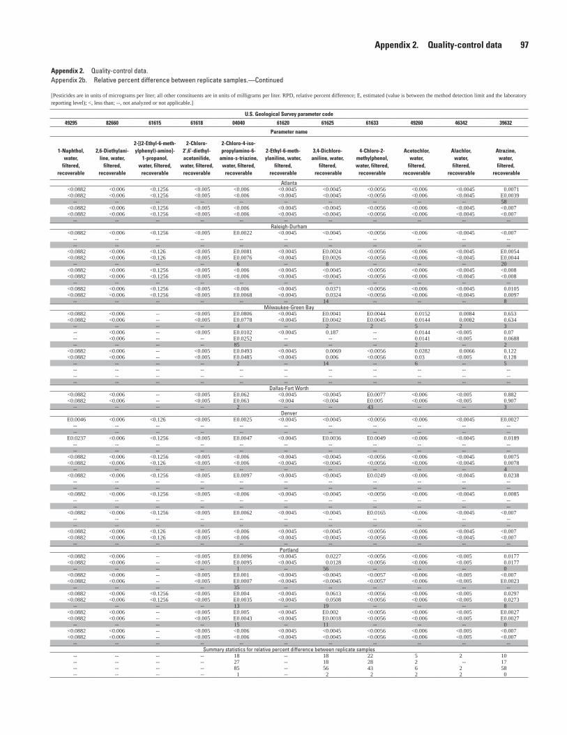
Appendix 2. Quality-control data. Appendix 2b. Relative percent difference between replicate samples.—Continued
[Pesticides are in units of micrograms per liter; all other constituents are in units of milligrams per liter. RPD, relative percent difference; E, estimated (value is between the method detection limit and the laboratory reporting level); <, less than; --, not analyzed or not applicable.]
U.S. Geological Survey parameter code
49295 82660 61615 61618 04040 61620 61625 61633 49260 46342 39632
Parameter name
1Naphthol, water,
filtered, recoverable
2,6Diethylaniline, water,
filtered, recoverable
2[(2Ethyl6methylphenyl)amino]
1propanol, water, filtered,
recoverable
2Chloro2’,6’diethylacetanilide,
water, filtered, recoverable
2Chloro4isopropylamino6
aminostriazine, water, filtered,
recoverable
2Ethyl6methylaniline, water,
filtered, recoverable
3,4Dichloroaniline, water,
filtered, recoverable
4Chloro2methylphenol, water, filtered,
recoverable
Acetochlor, water,
filtered, recoverable
Alachlor, water,
filtered, recoverable
Atrazine, water,
filtered, recoverable
Atlanta<0.0882 <0.006 <0.1256 <0.005 <0.006 <0.0045 <0.0045 <0.0056 <0.006 <0.0045 0.0071<0.0882 <0.006 <0.1256 <0.005 <0.006 <0.0045 <0.0045 <0.0056 <0.006 <0.0045 E0.0039
-- -- -- -- -- -- -- -- -- -- 58<0.0882 <0.006 <0.1256 <0.005 <0.006 <0.0045 <0.0045 <0.0056 <0.006 <0.0045 <0.007<0.0882 <0.006 <0.1256 <0.005 <0.006 <0.0045 <0.0045 <0.0056 <0.006 <0.0045 <0.007
-- -- -- -- -- -- -- -- -- -- --Raleigh-Durham
<0.0882 <0.006 <0.1256 <0.005 E0.0022 <0.0045 <0.0045 <0.0056 <0.006 <0.0045 <0.007-- -- -- -- -- -- -- -- -- -- ---- -- -- -- -- -- -- -- -- -- --
<0.0882 <0.006 <0.126 <0.005 E0.0081 <0.0045 E0.0024 <0.0056 <0.006 <0.0045 E0.0054<0.0882 <0.006 <0.126 <0.005 E0.0076 <0.0045 E0.0026 <0.0056 <0.006 <0.0045 E0.0044
-- -- -- -- 6 -- 8 -- -- -- 20<0.0882 <0.006 <0.1256 <0.005 <0.006 <0.0045 <0.0045 <0.0056 <0.006 <0.0045 <0.008<0.0882 <0.006 <0.1256 <0.005 <0.006 <0.0045 <0.0045 <0.0056 <0.006 <0.0045 <0.008
-- -- -- -- -- -- -- -- -- -- --<0.0882 <0.006 <0.1256 <0.005 <0.006 <0.0045 0.0371 <0.0056 <0.006 <0.0045 0.0105<0.0882 <0.006 <0.1256 <0.005 E0.0068 <0.0045 0.0324 <0.0056 <0.006 <0.0045 0.0097
-- -- -- -- -- -- 14 -- -- -- 8Milwaukee-Green Bay
<0.0882 <0.006 -- <0.005 E0.0806 <0.0045 E0.0041 E0.0044 0.0152 0.0084 0.653<0.0882 <0.006 -- <0.005 E0.0778 <0.0045 E0.0042 E0.0045 0.0144 0.0082 0.634
-- -- -- -- 4 -- 2 2 5 2 3-- <0.006 -- <0.005 E0.0102 <0.0045 0.187 -- 0.0144 <0.005 0.07-- <0.006 -- -- E0.0252 -- -- -- 0.0141 <0.005 0.0688-- -- -- -- 85 -- -- -- 2 -- 2
<0.0882 <0.006 -- <0.005 E0.0493 <0.0045 0.0069 <0.0056 0.0282 0.0066 0.122<0.0882 <0.006 -- <0.005 E0.0485 <0.0045 0.006 <0.0056 0.03 <0.005 0.128
-- -- -- -- 2 -- 14 -- 6 -- 5-- -- -- -- -- -- -- -- -- -- ---- -- -- -- -- -- -- -- -- -- ---- -- -- -- -- -- -- -- -- -- --
Dallas-Fort Worth<0.0882 <0.006 -- <0.005 E0.062 <0.0045 <0.0045 E0.0077 <0.006 <0.005 0.882<0.0882 <0.006 -- <0.005 E0.063 <0.004 <0.004 E0.005 <0.006 <0.005 0.907
-- -- -- -- 2 -- -- 43 -- -- 3Denver
E0.0046 <0.006 <0.126 <0.005 E0.0025 <0.0045 <0.0045 <0.0056 <0.006 <0.0045 E0.0027-- -- -- -- -- -- -- -- -- -- ---- -- -- -- -- -- -- -- -- -- --
E0.0237 <0.006 <0.1256 <0.005 E0.0047 <0.0045 E0.0036 E0.0049 <0.006 <0.0045 0.0189-- -- -- -- -- -- -- -- -- -- ---- -- -- -- -- -- -- -- -- -- --
<0.0882 <0.006 <0.1256 <0.005 <0.006 <0.0045 <0.0045 <0.0056 <0.006 <0.0045 0.0075<0.0882 <0.006 <0.126 <0.005 <0.006 <0.0045 <0.0045 <0.0056 <0.006 <0.0045 0.0078
-- -- -- -- -- -- -- -- -- -- 4<0.0882 <0.006 <0.1256 <0.005 E0.0097 <0.0045 <0.0045 E0.0249 <0.006 <0.0045 0.0238
-- -- -- -- -- -- -- -- -- -- ---- -- -- -- -- -- -- -- -- -- --
<0.0882 <0.006 <0.1256 <0.005 <0.006 <0.0045 <0.0045 <0.0056 <0.006 <0.0045 0.0085-- -- -- -- -- -- -- -- -- -- ---- -- -- -- -- -- -- -- -- -- --
<0.0882 <0.006 <0.1256 <0.005 E0.0062 <0.0045 <0.0045 E0.0165 <0.006 <0.0045 <0.007-- -- -- -- -- -- -- -- -- -- ---- -- -- -- -- -- -- -- -- -- --
<0.0882 <0.006 <0.126 <0.005 <0.006 <0.0045 <0.0045 <0.0056 <0.006 <0.0045 <0.007<0.0882 <0.006 <0.126 <0.005 <0.006 <0.0045 <0.0045 <0.0056 <0.006 <0.0045 <0.007
-- -- -- -- -- -- -- -- -- -- --Portland
<0.0882 <0.006 -- <0.005 E0.0096 <0.0045 0.0227 <0.0056 <0.006 <0.005 0.0177<0.0882 <0.006 -- <0.005 E0.0095 <0.0045 0.0128 <0.0056 <0.006 <0.005 0.0177
-- -- -- -- 1 -- 56 -- -- -- 0<0.0882 <0.006 -- <0.005 E0.001 <0.0045 <0.0045 <0.0057 <0.006 <0.005 <0.007<0.0882 <0.006 -- <0.005 E0.0007 <0.0045 <0.0045 <0.0057 <0.006 <0.005 E0.0023
-- -- -- -- 35 -- -- -- -- -- --<0.0882 <0.006 <0.1256 <0.005 E0.004 <0.0045 0.0613 <0.0056 <0.006 <0.005 0.0297<0.0882 <0.006 <0.1256 <0.005 E0.0035 <0.0045 0.0508 <0.0056 <0.006 <0.005 0.0273
-- -- -- -- 13 -- 19 -- -- -- 8<0.0882 <0.006 -- <0.005 E0.005 <0.0045 E0.002 <0.0056 <0.006 <0.005 E0.0027<0.0882 <0.006 -- <0.005 E0.0043 <0.0045 E0.0018 <0.0056 <0.006 <0.005 E0.0027
-- -- -- -- 15 -- 11 -- -- -- 0<0.0882 <0.006 -- <0.005 <0.006 <0.0045 <0.0045 <0.0056 <0.006 <0.005 <0.007<0.0882 <0.006 -- <0.005 <0.006 <0.0045 <0.0045 <0.0056 <0.006 <0.005 <0.007
-- -- -- -- -- -- -- -- -- -- --Summary statistics for relative percent difference between replicate samples
-- -- -- -- 18 -- 18 22 5 2 10-- -- -- -- 27 -- 18 28 2 -- 17-- -- -- -- 85 -- 56 43 6 2 58-- -- -- -- 1 -- 2 2 2 2 0
Appendix 2. Qualitycontrol data 97

98 Response of Stream Chemistry During Base Flow Across United States, 2002–04
Appendix 2. Quality-control data. Appendix 2b. Relative percent difference between replicate samples. —Continued
[Pesticides are in units of micrograms per liter; all other constituents are in units of milligrams per liter. RPD, relative percent difference; E, estimated (value is between the method detection limit and the laboratory reporting level); <, less than; --, not analyzed or not applicable.]
U.S. Geological Survey station
numberU.S. Geological Survey
station name
Sample date
and time Variable
U.S. Geological Survey parameter code61635 82686 82673 82680 61636
Parameter nameAzinphos
methyl oxygen analog, water, filtered, recov
erable
Azinphosmethyl, water,
filtered, recoverable
Benfluralin, water,
filtered, recoverable
Carbaryl, water,
filtered,recoverable
Chlorpyrifos oxygen analog, water, filtered,
recoverable
Atlanta02337395 Dog River at North Helton Road near Winston, Ga. 2003-07-08 1200 replicate <0.125 <0.05 <0.01 E0.0074 <0.056202337395 Dog River at North Helton Road near Winston, Ga. 2003-07-08 1207 replicate <0.016 <0.05 <0.01 E0.0068 <0.0562
RPD -- -- -- 8 --02346358 Turnpike Creek near Milner, Ga. 2003-09-17 0930 replicate -- <0.05 <0.01 <0.041 <0.056202346358 Turnpike Creek near Milner, Ga. 2003-09-17 0937 replicate -- <0.05 <0.01 <0.041 <0.0562
RPD -- -- -- -- --Raleigh-Durham
0208500600 Strouds Creek at St Marys Road near Hillsborough, N.C. 2003-07-07 0830 replicate <0.016 <0.05 <0.01 E0.0089 <0.05620208500600 Strouds Creek at St Marys Road near Hillsborough, N.C. 2003-07-07 0831 replicate -- -- -- -- --
RPD -- -- -- -- --0208732610 Pigeon House Br at Crabtree Boulevard at Raleigh, N.C. 2002-12-19 1100 replicate <0.016 <0.05 <0.01 E0.0036 <0.05620208732610 Pigeon House Br at Crabtree Boulevard at Raleigh, N.C. 2002-12-19 1101 replicate <0.016 <0.05 <0.01 E0.0038 <0.0562
RPD -- -- -- 5 --02100634 Vestal Creek near Asheboro, N.C. 2003-07-08 0915 replicate <0.016 <0.05 <0.01 <0.041 <0.056202100634 Vestal Creek near Asheboro, N.C. 2003-07-08 0916 replicate <0.016 <0.05 <0.01 <0.041 <0.0562
RPD -- -- -- -- --0211583580 Bowen Branch near Mouth at Winston-Salem, N.C. 2003-07-09 1030 replicate <0.016 <0.05 <0.01 <0.041 <0.05620211583580 Bowen Branch near Mouth at Winston-Salem, N.C. 2003-07-09 1031 replicate <0.016 <0.05 <0.01 <0.041 <0.0562
RPD -- -- -- -- --Milwaukee-Green Bay
04081897 Sawyer Creek at Westhaven Road at Oshkosh, Wis. 2004-05-19 0930 replicate <0.016 <0.05 <0.01 E0.0125 <0.056204081897 Sawyer Creek at Westhaven Road at Oshkosh, Wis. 2004-05-19 0931 replicate <0.016 <0.05 <0.01 E0.0146 <0.0562
RPD -- -- -- 15 --040869415 Lincoln Creek at 47th Street at Milwaukee, Wis. 2004-06-01 1320 replicate <0.016 <0.05 <0.01 E0.0083 <0.0562040869415 Lincoln Creek at 47th Street at Milwaukee, Wis. 2004-06-01 1321 replicate -- <0.05 <0.01 E0.0078 --
RPD -- -- -- 6 --04087030 Menomonee River at Menomonee Falls, Wis. 2004-06-10 1210 replicate <0.016 <0.05 <0.01 E0.0073 <0.056204087030 Menomonee River at Menomonee Falls, Wis. 2004-06-10 1211 replicate <0.016 <0.05 <0.01 E0.0075 <0.0562
RPD -- -- -- 3 --04087204 Oak Creek at South Milwaukee, Wis. 2004-05-13 1141 replicate -- -- -- -- --04087204 Oak Creek at South Milwaukee, Wis. 2004-05-13 1142 replicate -- -- -- -- --
RPD -- -- -- -- --Dallas-Fort Worth
08049955 Fish Creek at Belt Line Road, Grand Prairie, Tex. 2004-05-20 1505 replicate <0.03 <0.05 <0.01 E0.0541 <0.056208049955 Fish Creek at Belt Line Road, Grand Prairie, Tex. 2004-05-20 1506 replicate <0.02 <0.05 <0.01 E0.06 <0.06
RPD -- -- -- 10 --Denver
393948105053501 Bear Creek below Estes Road at Lakewood, Colo. 2003-02-10 1245 replicate <0.016 <0.05 <0.01 <0.041 <0.0562393948105053501 Bear Creek below Estes Road at Lakewood, Colo. 2003-02-10 1246 replicate -- -- -- -- --
RPD -- -- -- -- --394409105020501 Lakewood Gulch above Knox Street at Denver, Colo. 2003-08-13 1100 replicate <0.016 <0.05 <0.01 E0.13 <0.0562394409105020501 Lakewood Gulch above Knox Street at Denver, Colo. 2003-08-13 1101 replicate -- -- -- -- --
RPD -- -- -- -- --394921105015701 Little Dry Creek below Lowell Street near Westminster, Colo. 2002-12-11 0930 replicate <0.016 <0.05 <0.01 <0.041 <0.0562394921105015701 Little Dry Creek below Lowell Street near Westminster, Colo. 2002-12-11 0931 replicate <0.016 <0.05 <0.01 <0.041 <0.0562
RPD -- -- -- -- --395554105085601 Rock Creek above Rock Creek Parkway at Superior, Colo. 2003-08-21 1145 replicate <0.016 <0.05 <0.01 E0.0095 <0.0562395554105085601 Rock Creek above Rock Creek Parkway at Superior, Colo. 2003-08-21 1146 replicate -- -- -- -- --
RPD -- -- -- -- --400217105123701 Boulder Creek below 61st Street near Boulder, Colo. 2002-12-10 0950 replicate <0.016 <0.05 <0.01 E0.0083 <0.0562400217105123701 Boulder Creek below 61st Street near Boulder, Colo. 2002-12-10 0951 replicate -- -- -- -- --
RPD -- -- -- -- --403356105024001 Spring Creek at Edora Park at Fort Collins, Colo. 2003-08-27 1130 replicate <0.016 <0.05 <0.01 E0.0061 <0.0562403356105024001 Spring Creek at Edora Park at Fort Collins, Colo. 2003-08-27 1131 replicate -- -- -- -- --
RPD -- -- -- -- --413659104370001 Bear Creek above Little Bear Creek near Phillips, Wyo. 2003-04-02 1100 replicate <0.016 <0.05 <0.01 <0.041 <0.0562413659104370001 Bear Creek above Little Bear Creek near Phillips, Wyo. 2003-04-02 1101 replicate <0.016 <0.05 <0.01 <0.041 <0.0562
RPD -- -- -- -- --Portland
450022123012400 Claggett Creek at Keizer, Oreg. 2004-05-13 1250 replicate <0.016 <0.05 <0.01 E0.0096 <0.0562450022123012400 Claggett Creek at Keizer, Oreg. 2004-05-13 1251 replicate <0.016 <0.05 <0.01 E0.0096 <0.0562
RPD -- -- -- 0 --452231122200000 Deep Creek near Sandy, Oreg. 2004-08-17 1200 replicate <0.07 <0.05 <0.01 <0.041 <0.0562452231122200000 Deep Creek near Sandy, Oreg. 2004-08-17 1201 replicate <0.07 <0.05 <0.01 <0.041 <0.0562
RPD -- -- -- -- --452337122243500 North Fork Deep Creek at Barton, Oreg. 2004-01-14 1150 replicate <0.031 <0.05 <0.01 E0.0068 <0.0562452337122243500 North Fork Deep Creek at Barton, Oreg. 2004-01-14 1151 replicate <0.031 <0.05 <0.01 E0.0073 <0.0562
RPD -- -- -- 7 --452526122364400 Kellogg Creek at Milwaukie, Oreg. 2004-03-10 1150 replicate <0.016 <0.05 <0.01 E0.0232 <0.0562452526122364400 Kellogg Creek at Milwaukie, Oreg. 2004-03-10 1151 replicate <0.016 <0.05 <0.01 E0.0208 <0.0562
RPD -- -- -- 11 --454510122424900 Whipple Creek near Salmon Creek, Wash. 2004-06-28 1140 replicate <0.016 <0.05 <0.01 <0.041 <0.0562454510122424900 Whipple Creek near Salmon Creek, Wash. 2004-06-28 1141 replicate <0.016 <0.05 <0.01 <0.041 <0.0562
RPD -- -- -- -- --Summary statistics for relative percent difference between replicate samples
Mean -- -- -- 7 --Standard deviation -- -- -- 5 --Maximum -- -- -- 15 --Minimum -- -- -- 0 --

Appendix 2. Quality-control data. Appendix 2b. Relative percent difference between replicate samples.—Continued [Pesticides are in units of micrograms per liter; all other constituents are in units of milligrams per liter. RPD, relative percent difference; E, estimated (value is between the method detection limit and the laboratory reporting level); <, less than; --, not analyzed or not applicable.]
U.S. Geological Survey parameter code38933 82687 61585 61586 82682 62170 61638 39572 38454 39381 82662
Parameter name
Chlorpyrifos, water,
filtered, recoverable
cisPermethrin, water,
filtered, recoverable
Cyfluthrin, water,
filtered, recoverable
Cypermethrin, water,
filtered, recoverable
DCPA, water,
filtered, recoverable
Desulfinyl fipronil, water,
filtered, recoverable
Diazinon oxygen analog, water,
filtered, recoverable
Diazinon, water,
filtered, recoverable
Dicrotophos, water,
filtered, recoverable
Dieldrin, water,
filtered, recoverable
Dimethoate, water,
filtered, recoverable
Atlanta<0.005 <0.006 <0.008 <0.0086 <0.003 <0.004 <0.01 <0.005 <0.0843 <0.0048 <0.0061<0.005 <0.006 <0.008 <0.0086 <0.003 <0.004 <0.01 <0.005 <0.0843 <0.0048 <0.0061
-- -- -- -- -- -- -- -- -- -- --<0.005 <0.006 <0.008 <0.0086 <0.003 <0.004 <0.01 <0.005 <0.0843 <0.0048 <0.0061<0.005 <0.006 <0.008 <0.0086 <0.003 <0.004 <0.01 <0.005 <0.0843 <0.0048 <0.0061
-- -- -- -- -- -- -- -- -- -- --Raleigh-Durham
<0.005 <0.006 <0.008 <0.0086 <0.003 <0.004 <0.01 <0.005 <0.0843 <0.0048 <0.0061-- -- -- -- -- -- -- -- -- -- ---- -- -- -- -- -- -- -- -- -- --
<0.005 <0.006 <0.008 <0.0086 <0.003 <0.004 <0.04 <0.005 <0.0843 0.0082 <0.0061<0.005 <0.006 <0.008 <0.0086 <0.003 <0.004 <0.04 <0.005 <0.0843 0.0068 <0.0061
-- -- -- -- -- -- -- -- -- 19 --<0.005 <0.006 <0.008 <0.0086 <0.003 <0.004 <0.01 <0.005 <0.0843 <0.0048 <0.0061<0.005 <0.006 <0.008 <0.0086 <0.003 <0.004 <0.01 <0.005 <0.0843 <0.0048 <0.0061
-- -- -- -- -- -- -- -- -- -- --<0.005 <0.006 <0.008 <0.0086 <0.003 <0.004 <0.01 <0.005 <0.0843 0.0076 <0.0061<0.005 <0.006 <0.008 <0.0086 <0.003 <0.004 <0.01 <0.005 <0.0843 <0.0048 <0.0061
-- -- -- -- -- -- -- -- -- -- --Milwaukee-Green Bay
<0.005 <0.006 <0.008 <0.0086 <0.003 <0.012 <0.01 <0.005 <0.0843 <0.009 <0.0061<0.005 <0.006 <0.008 <0.0086 <0.003 <0.012 <0.01 <0.005 <0.0843 <0.009 <0.0061
-- -- -- -- -- -- -- -- -- -- --<0.005 <0.006 <0.008 <0.0086 <0.003 <0.012 -- 0.0054 <0.0843 <0.009 <0.0061<0.005 <0.006 -- -- <0.003 <0.012 -- E0.0037 -- <0.009 --
-- -- -- -- -- -- -- 37 -- -- --<0.005 <0.006 <0.008 <0.0086 <0.003 <0.012 <0.01 <0.009 <0.0843 <0.009 <0.0061<0.005 <0.006 <0.008 <0.0086 <0.003 <0.012 <0.01 <0.009 <0.0843 <0.009 <0.0061
-- -- -- -- -- -- -- -- -- -- ---- -- -- -- -- -- -- -- -- -- ---- -- -- -- -- -- -- -- -- -- ---- -- -- -- -- -- -- -- -- -- --
Dallas-Fort Worth0.0069 <0.006 <0.008 <0.0086 <0.003 E0.0033 <0.01 0.0175 <0.0843 <0.009 <0.00610.006 <0.006 <0.008 <0.009 <0.003 E0.004 <0.01 0.019 <0.08 <0.009 <0.006
14 -- -- -- -- 19 -- 8 -- -- --Denver
<0.005 <0.006 <0.008 <0.0086 <0.003 <0.004 <0.04 <0.005 <0.0843 <0.0048 <0.0061-- -- -- -- -- -- -- -- -- -- ---- -- -- -- -- -- -- -- -- -- --
<0.005 <0.006 <0.008 <0.0086 <0.003 <0.004 <0.01 0.0063 <0.0843 <0.0048 <0.0061-- -- -- -- -- -- -- -- -- -- ---- -- -- -- -- -- -- -- -- -- --
<0.005 <0.006 <0.008 <0.0086 <0.003 <0.004 <0.04 0.0066 <0.0843 <0.0048 <0.0061<0.005 <0.006 <0.008 <0.0086 <0.003 <0.004 <0.04 0.0069 <0.0843 <0.0048 <0.0061
-- -- -- -- -- -- -- 4 -- -- --<0.005 <0.006 <0.008 <0.0086 E0.0011 <0.004 <0.01 0.009 <0.0843 <0.0048 <0.007
-- -- -- -- -- -- -- -- -- -- ---- -- -- -- -- -- -- -- -- -- --
<0.005 <0.006 <0.008 <0.0086 <0.003 <0.004 <0.04 <0.005 <0.0843 <0.0048 <0.0061-- -- -- -- -- -- -- -- -- -- ---- -- -- -- -- -- -- -- -- -- --
<0.005 <0.006 <0.008 <0.0086 <0.003 <0.004 <0.01 <0.005 <0.0843 <0.0048 <0.0061-- -- -- -- -- -- -- -- -- -- ---- -- -- -- -- -- -- -- -- -- --
<0.005 <0.006 <0.008 <0.0086 <0.003 <0.004 <0.04 <0.005 <0.0843 <0.0048 <0.0061<0.005 <0.006 <0.008 <0.0086 <0.003 <0.004 <0.04 <0.005 <0.0843 <0.0048 <0.0061
-- -- -- -- -- -- -- -- -- -- --Portland
<0.005 <0.006 <0.008 <0.0086 <0.003 <0.012 <0.01 <0.005 <0.0843 <0.009 <0.0061<0.005 <0.006 <0.008 <0.0086 <0.003 <0.012 <0.01 <0.005 <0.0843 <0.009 <0.0061
-- -- -- -- -- -- -- -- -- -- --<0.005 <0.006 <0.008 <0.0086 <0.003 <0.012 <0.006 <0.005 <0.0843 <0.009 <0.0061<0.005 <0.006 <0.008 <0.0086 <0.003 <0.012 <0.006 <0.005 <0.0843 <0.009 <0.0061
-- -- -- -- -- -- -- -- -- -- --0.0134 <0.006 <0.008 <0.0086 <0.003 <0.012 <0.01 <0.005 <0.0843 E0.0023 <0.00610.0126 <0.006 <0.008 <0.0086 <0.003 <0.012 <0.01 <0.005 <0.0843 E0.003 <0.00616 -- -- -- -- -- -- -- -- 26 --
<0.005 <0.006 <0.008 <0.0086 <0.003 <0.012 <0.01 <0.005 <0.0843 <0.009 <0.0061<0.005 <0.006 <0.008 <0.0086 <0.003 <0.012 <0.01 <0.005 <0.0843 <0.009 <0.0061
-- -- -- -- -- -- -- -- -- -- --<0.005 <0.006 <0.03 <0.03 <0.003 <0.012 <0.01 <0.005 <0.0843 <0.009 <0.0061<0.005 <0.006 <0.03 <0.03 <0.003 <0.012 <0.01 <0.005 <0.0843 <0.009 <0.0061
-- -- -- -- -- -- -- -- -- -- --Summary statistics for relative percent difference between replicate samples
10 -- -- -- -- 19 -- 17 -- 23 --6 -- -- -- -- -- -- 18 -- 5 --
14 -- -- -- -- 19 -- 37 -- 26 --6 -- -- -- -- 19 -- 4 -- 19 --
Appendix 2. Qualitycontrol data 99

100 Response of Stream Chemistry During Base Flow Across United States, 2002–04
Appendix 2. Quality-control data. Appendix 2b. Relative percent difference between replicate samples.—Continued
[Pesticides are in units of micrograms per liter; all other constituents are in units of milligrams per liter. RPD, relative percent difference; E, estimated (value is between the method detection limit and the laboratory reporting level); <, less than; --, not analyzed or not applicable.]
U.S. Geological Survey
station number
U.S. Geological Survey station name
Sample date and time
Variable
U.S. Geological Survey parameter code61644 82346 61645 61646 61591
Parameter nameEthion
monoxon,water,
filtered, recoverable
Ethion, water,
filtered, recoverable
Fenamiphos sulfone,
water, filtered, recoverable
Fenamiphos sulfoxide, water,
filtered, recoverable
Fenamiphos, water,
filtered, recoverable
Atlanta02337395 Dog River at North Helton Road near Winston, Ga. 2003-07-08 1200 replicate <0.0336 <0.004 <0.0077 <0.125 <0.02902337395 Dog River at North Helton Road near Winston, Ga. 2003-07-08 1207 replicate <0.0336 <0.004 <0.0077 <0.031 <0.029
RPD -- -- -- -- --02346358 Turnpike Creek near Milner, Ga. 2003-09-17 0930 replicate <0.0336 <0.004 <0.0077 -- <0.02902346358 Turnpike Creek near Milner, Ga. 2003-09-17 0937 replicate <0.0336 <0.004 <0.0077 -- <0.029
RPD -- -- -- -- --Raleigh-Durham
0208500600 Strouds Creek at St Marys Road near Hillsborough, N.C. 2003-07-07 0830 replicate <0.0336 <0.004 <0.0077 <0.031 <0.0290208500600 Strouds Creek at St Marys Road near Hillsborough, N.C. 2003-07-07 0831 replicate -- -- -- -- --
RPD -- -- -- -- --0208732610 Pigeon House Br at Crabtree Boulevard at Raleigh, N.C. 2002-12-19 1100 replicate <0.0336 <0.004 <0.0077 <0.031 <0.0290208732610 Pigeon House Br at Crabtree Boulevard at Raleigh, N.C. 2002-12-19 1101 replicate <0.0336 <0.004 <0.0077 <0.031 <0.029
RPD -- -- -- -- --02100634 Vestal Creek near Asheboro, N.C. 2003-07-08 0915 replicate <0.0336 <0.004 <0.0312 <0.031 <0.02902100634 Vestal Creek near Asheboro, N.C. 2003-07-08 0916 replicate <0.0336 <0.004 <0.0312 <0.031 <0.029
RPD -- -- -- --0211583580 Bowen Branch near Mouth at Winston-Salem, N.C. 2003-07-09 1030 replicate <0.0336 <0.004 <0.0077 <0.031 <0.0290211583580 Bowen Branch near Mouth at Winston-Salem, N.C. 2003-07-09 1031 replicate <0.0336 <0.004 <0.0077 <0.031 <0.029
RPD -- -- -- -- --Milwaukee-Green Bay
04081897 Sawyer Creek at Westhaven Road at Oshkosh, Wis. 2004-05-19 0930 replicate <0.0336 <0.004 <0.0077 <0.031 <0.02904081897 Sawyer Creek at Westhaven Road at Oshkosh, Wis. 2004-05-19 0931 replicate <0.0336 <0.004 <0.0077 <0.031 <0.029
RPD -- -- -- -- --040869415 Lincoln Creek at 47th Street at Milwaukee, Wis. 2004-06-01 1320 replicate <0.0336 <0.004 <0.0077 <0.031 <0.029040869415 Lincoln Creek at 47th Street at Milwaukee, Wis. 2004-06-01 1321 replicate -- -- -- -- --
RPD -- -- -- -- --04087030 Menomonee River at Menomonee Falls, Wis. 2004-06-10 1210 replicate <0.0336 <0.004 <0.0077 <0.031 <0.02904087030 Menomonee River at Menomonee Falls, Wis. 2004-06-10 1211 replicate <0.0336 <0.004 <0.0077 <0.031 <0.029
RPD -- -- -- -- --04087204 Oak Creek at South Milwaukee, Wis. 2004-05-13 1141 replicate -- -- -- -- --04087204 Oak Creek at South Milwaukee, Wis. 2004-05-13 1142 replicate -- -- -- -- --
RPD -- -- -- -- --Dallas-Fort Worth
08049955 Fish Creek at Belt Line Road, Grand Prairie, Tex. 2004-05-20 1505 replicate <0.0336 <0.004 <0.03 -- <0.02908049955 Fish Creek at Belt Line Road, Grand Prairie, Tex. 2004-05-20 1506 replicate <0.03 <0.004 <0.03 -- <0.03
RPD -- -- -- -- --Denver
393948105053501 Bear Creek below Estes Road at Lakewood, Colo. 2003-02-10 1245 replicate <0.0336 <0.004 <0.0077 <0.031 <0.029393948105053501 Bear Creek below Estes Road at Lakewood, Colo. 2003-02-10 1246 replicate -- -- -- -- --
RPD -- -- -- -- --394409105020501 Lakewood Gulch above Knox Street at Denver, Colo. 2003-08-13 1100 replicate <0.0336 <0.004 <0.0077 <0.031 <0.029394409105020501 Lakewood Gulch above Knox Street at Denver, Colo. 2003-08-13 1101 replicate -- -- -- -- --
RPD -- -- -- -- --394921105015701 Little Dry Creek below Lowell Street near Westminster, Colo. 2002-12-11 0930 replicate <0.0336 <0.004 <0.0077 <0.031 <0.029394921105015701 Little Dry Creek below Lowell Street near Westminster, Colo. 2002-12-11 0931 replicate <0.0336 <0.004 <0.0077 <0.031 <0.029
RPD -- -- -- -- --395554105085601 Rock Creek above Rock Creek Parkway at Superior, Colo. 2003-08-21 1145 replicate <0.0336 <0.004 <0.0077 <0.031 <0.029395554105085601 Rock Creek above Rock Creek Parkway at Superior, Colo. 2003-08-21 1146 replicate -- -- -- -- --
RPD -- -- -- -- --400217105123701 Boulder Creek below 61st Street near Boulder, Colo. 2002-12-10 0950 replicate <0.0336 <0.004 <0.0077 <0.031 <0.029400217105123701 Boulder Creek below 61st Street near Boulder, Colo. 2002-12-10 0951 replicate -- -- -- -- --
RPD -- -- -- -- --403356105024001 Spring Creek at Edora Park at Fort Collins, Colo. 2003-08-27 1130 replicate <0.0336 <0.004 <0.0077 <0.031 <0.029403356105024001 Spring Creek at Edora Park at Fort Collins, Colo. 2003-08-27 1131 replicate -- -- -- -- --
RPD -- -- -- -- --413659104370001 Bear Creek above Little Bear Creek near Phillips, Wyo. 2003-04-02 1100 replicate <0.0336 <0.004 <0.0077 <0.031 <0.029413659104370001 Bear Creek above Little Bear Creek near Phillips, Wyo. 2003-04-02 1101 replicate <0.0336 <0.004 <0.0077 <0.031 <0.029
RPD -- -- -- -- --Portland
450022123012400 Claggett Creek at Keizer, Oreg. 2004-05-13 1250 replicate <0.0336 <0.004 <0.0077 <0.031 <0.029450022123012400 Claggett Creek at Keizer, Oreg. 2004-05-13 1251 replicate <0.0336 <0.004 <0.0077 <0.031 <0.029
RPD -- -- -- -- --452231122200000 Deep Creek near Sandy, Oreg. 2004-08-17 1200 replicate <0.002 <0.004 <0.0491 <0.0387 <0.029452231122200000 Deep Creek near Sandy, Oreg. 2004-08-17 1201 replicate <0.002 <0.004 <0.0491 <0.0387 <0.029
RPD -- -- -- -- --452337122243500 North Fork Deep Creek at Barton, Oreg. 2004-01-14 1150 replicate <0.0336 <0.004 <0.0077 <0.031 <0.029452337122243500 North Fork Deep Creek at Barton, Oreg. 2004-01-14 1151 replicate <0.0336 <0.004 <0.0077 <0.031 <0.029
RPD -- -- -- -- --452526122364400 Kellogg Creek at Milwaukie, Oreg. 2004-03-10 1150 replicate <0.0336 <0.004 <0.0077 <0.031 <0.029452526122364400 Kellogg Creek at Milwaukie, Oreg. 2004-03-10 1151 replicate <0.0336 <0.004 <0.0077 <0.031 <0.029
RPD -- -- -- -- --454510122424900 Whipple Creek near Salmon Creek, Wash. 2004-06-28 1140 replicate <0.0336 <0.004 <0.0077 <0.031 <0.029454510122424900 Whipple Creek near Salmon Creek, Wash. 2004-06-28 1141 replicate <0.0336 <0.004 <0.0077 <0.031 <0.029
RPD -- -- -- -- --Summary statistics for relative percent difference between replicate samples
Mean -- -- -- -- --Standard deviation -- -- -- -- --Maximum -- -- -- -- --Minimum -- -- -- -- --

Appendix 2. Quality-control data. Appendix 2b. Relative percent difference between replicate samples.—Continued
[Pesticides are in units of micrograms per liter; all other constituents are in units of milligrams per liter. RPD, relative percent difference; E, estimated (value is between the method detection limit and the labora-tory reporting level); <, less than; --, not analyzed or not applicable.]
U.S. Geological Survey parameter code62169 62167 62168 62166 61649 04095 04025 61593 61594 61652 39532
Parameter name
Desulfinylfipronil amide, water,
filtered, recoverable
Fipronil sulfide, water, filtered,
recoverable
Fipronil sulfone, water, filtered,
recoverable
Fipronil, water, filtered,
recoverable
Fonofos oxygen analog, water,
filtered, recoverable
Fonofos, water, filtered,
recoverable
Hexazinone, water, filtered,
recoverable
Iprodione, water,
filtered, recoverable
Isofenphos, water,
filtered, recoverable
Malaoxon, water,
filtered, recoverable
Malathion, water,
filtered, recoverable
Atlanta<0.009 <0.005 <0.005 <0.007 <0.0021 <0.0027 <0.0129 <1.4223 <0.0034 <0.008 <0.027<0.009 <0.005 <0.005 <0.007 <0.0021 <0.0027 <0.0129 <1.4223 <0.0034 <0.008 <0.027
-- -- -- -- -- -- -- -- -- -- --<0.009 <0.005 <0.005 <0.007 <0.0021 <0.0027 E0.0066 <1.4223 <0.0034 <0.008 <0.027<0.009 <0.005 <0.005 <0.007 <0.0021 <0.0027 E0.0065 <1.4223 <0.0034 <0.008 <0.027
-- -- -- -- -- -- 2 -- -- -- --Raleigh-Durham
<0.009 <0.005 <0.005 <0.007 <0.0021 <0.0027 0.0166 <1.4223 <0.0034 <0.008 <0.027-- -- -- -- -- -- -- -- -- -- ---- -- -- -- -- -- -- -- -- -- --
<0.009 <0.005 <0.005 E0.0052 <0.0021 <0.0027 -- <1.4223 <0.0034 <0.008 <0.027<0.009 <0.005 <0.005 E0.0053 <0.0021 <0.0027 -- <1.4223 <0.0034 <0.008 <0.027
-- -- -- 2 -- -- -- -- -- -- --<0.009 <0.005 <0.006 E0.0053 <0.0021 <0.0027 0.0391 <1.4223 <0.0034 <0.008 <0.027<0.009 <0.005 <0.006 <0.007 <0.0021 <0.0027 0.0373 <1.4223 <0.0034 <0.008 <0.027
-- -- -- -- -- -- 5 -- -- -- --<0.009 <0.005 <0.005 <0.007 <0.0021 <0.0027 0.0177 <1.4223 <0.0034 <0.008 <0.027<0.009 <0.005 <0.005 <0.007 <0.0021 <0.0027 0.0176 <1.4223 <0.0034 <0.008 <0.027
-- -- -- -- -- -- 1 -- -- -- --Milwaukee-Green Bay
<0.029 <0.013 <0.024 <0.016 <0.0021 <0.003 <0.0129 <1.4223 <0.0034 <0.008 E0.0158<0.029 <0.013 <0.024 <0.016 <0.0021 <0.003 <0.0129 <1.4223 <0.0034 <0.008 E0.0156
-- -- -- -- -- -- -- -- -- -- 1<0.029 <0.013 <0.024 <0.016 <0.0021 <0.003 <0.0129 <1.4223 <0.0034 <0.008 <0.027<0.029 <0.013 <0.024 <0.016 -- <0.003 -- -- -- -- <0.027
-- -- -- -- -- -- -- -- -- -- --<0.029 <0.013 <0.024 <0.016 <0.0021 <0.003 <0.0129 <1.4223 <0.0034 <0.008 <0.027<0.029 <0.013 <0.024 <0.016 <0.0021 <0.003 <0.0129 <1.4223 <0.0034 <0.008 <0.027
-- -- -- -- -- -- -- -- -- -- ---- -- -- -- -- -- -- -- -- -- ---- -- -- -- -- -- -- -- -- -- ---- -- -- -- -- -- -- -- -- -- --
Dallas-Fort Worth<0.029 <0.013 <0.024 E0.0095 <0.0021 <0.003 0.0154 <1.4223 <0.0034 <0.008 <0.027<0.029 <0.013 <0.024 E0.01 <0.002 <0.003 0.019 <1.4223 <0.003 <0.008 <0.027
-- -- -- 5 -- -- 21 -- -- -- --Denver
<0.009 <0.005 <0.005 <0.007 <0.0021 <0.0027 -- <1.4223 <0.0034 <0.008 <0.027-- -- -- -- -- -- -- -- -- -- ---- -- -- -- -- -- -- -- -- -- --
<0.009 <0.005 <0.005 <0.007 <0.0021 <0.0027 <0.0129 <1.4223 <0.0034 <0.008 <0.027-- -- -- -- -- -- -- -- -- -- ---- -- -- -- -- -- -- -- -- -- --
<0.009 <0.005 <0.005 <0.007 <0.0021 <0.0027 -- <1.4223 <0.0034 <0.008 <0.027<0.009 <0.005 <0.005 <0.007 <0.0021 <0.0027 -- <1.4223 <0.0034 <0.008 <0.027
-- -- -- -- -- -- -- -- -- -- --<0.009 <0.005 <0.005 <0.007 <0.0021 <0.0027 <0.0129 <1.4223 <0.0034 <0.008 <0.027
-- -- -- -- -- -- -- -- -- -- ---- -- -- -- -- -- -- -- -- -- --
<0.009 <0.005 <0.005 <0.007 <0.0021 <0.0027 -- <1.4223 <0.0034 <0.008 <0.027-- -- -- -- -- -- -- -- -- -- ---- -- -- -- -- -- -- -- -- -- --
<0.009 <0.005 <0.005 <0.007 <0.0021 <0.0027 <0.0129 <1.4223 <0.0034 <0.008 <0.027-- -- -- -- -- -- -- -- -- -- ---- -- -- -- -- -- -- -- -- -- --
<0.009 <0.005 <0.005 <0.007 <0.0021 <0.0027 -- <1.4223 <0.0034 <0.008 <0.027<0.009 <0.005 <0.005 <0.007 <0.0021 <0.0027 -- <1.4223 <0.0034 <0.008 <0.027
-- -- -- -- -- -- -- -- -- -- --Portland
<0.029 <0.013 <0.024 <0.016 <0.0021 <0.003 <0.0129 <1.4223 <0.0034 <0.008 <0.027<0.029 <0.013 <0.024 <0.016 <0.0021 <0.003 <0.0129 <1.4223 <0.0034 <0.008 <0.027
-- -- -- -- -- -- -- -- -- -- --<0.029 <0.013 <0.024 <0.016 <0.0029 <0.003 0.0172 <0.387 <0.0034 <0.0298 <0.027<0.029 <0.013 <0.024 <0.016 <0.0029 <0.003 0.0147 <0.387 <0.0034 <0.0298 <0.027
-- -- -- -- -- -- 16 -- -- -- --<0.029 <0.013 <0.024 <0.016 <0.0021 <0.003 0.0159 <1.4223 <0.0034 <0.008 <0.027<0.029 <0.013 <0.024 <0.016 <0.0021 <0.003 0.0149 <1.4223 <0.0034 <0.008 <0.027
-- -- -- -- -- -- 6 -- -- -- --<0.029 <0.013 <0.024 <0.016 <0.0021 <0.003 <0.0129 <1.4223 <0.0034 <0.008 <0.027<0.029 <0.013 <0.024 <0.016 <0.0021 <0.003 <0.0129 <1.4223 <0.0034 <0.008 <0.027
-- -- -- -- -- -- -- -- -- -- --<0.029 <0.013 <0.024 <0.016 <0.0021 <0.003 <0.0129 <1.4223 <0.0034 <0.008 <0.027<0.029 <0.013 <0.024 <0.016 <0.0021 <0.003 <0.0129 <1.4223 <0.0034 <0.008 <0.027
-- -- -- -- -- -- -- -- -- -- --Summary statistics for relative percent difference between replicate samples
-- -- -- 4 -- -- 8 -- -- -- 1-- -- -- 2 -- -- 8 -- -- -- ---- -- -- 5 -- -- 21 -- -- -- 1-- -- -- 2 -- -- 1 -- -- -- 1
Appendix 2. Qualitycontrol data 101

102 Response of Stream Chemistry During Base Flow Across United States, 2002–04
Appendix 2. Quality-control data. Appendix 2b. Relative percent difference between replicate samples.—Continued
[Pesticides are in units of micrograms per liter; all other constituents are in units of milligrams per liter. RPD, relative percent difference; E, estimated (value is between the method detection limit and the laboratory reporting level); <, less than; --, not analyzed or not applicable.]
U.S. Geological Survey
station numberU.S. Geological Survey
station name
Sample date
and time Variable
U.S. Geological Survey parameter code61596 61598 61664 82667 39415
Parameter name
Metalaxyl, water,
filtered, recoverable
Methidathion, water,
filtered, recoverable
Methyl paraoxon,
water, filtered,
recoverable
Methyl parathion,
water, filtered,
recoverable
Metolachlor, water,
filtered, recoverable
Atlanta02337395 Dog River at North Helton Road near Winston, Ga. 2003-07-08 1200 replicate <0.0051 <0.0058 <0.0299 <0.006 <0.01302337395 Dog River at North Helton Road near Winston, Ga. 2003-07-08 1207 replicate <0.0051 <0.0058 <0.0299 <0.006 <0.013
RPD -- -- -- -- --02346358 Turnpike Creek near Milner, Ga. 2003-09-17 0930 replicate <0.0051 <0.0058 <0.0299 <0.006 <0.01302346358 Turnpike Creek near Milner, Ga. 2003-09-17 0937 replicate <0.0051 <0.0058 <0.0299 <0.006 <0.013
RPD -- -- -- -- --Raleigh-Durham
0208500600 Strouds Creek at St Marys Road near Hillsborough, N.C. 2003-07-07 0830 replicate <0.0051 <0.0058 <0.0299 <0.006 <0.0130208500600 Strouds Creek at St Marys Road near Hillsborough, N.C. 2003-07-07 0831 replicate -- -- -- -- --
RPD -- -- -- -- --0208732610 Pigeon House Br at Crabtree Boulevard at Raleigh, N.C. 2002-12-19 1100 replicate <0.0051 <0.0058 <0.0299 <0.006 0.05410208732610 Pigeon House Br at Crabtree Boulevard at Raleigh, N.C. 2002-12-19 1101 replicate <0.0051 <0.0058 <0.0299 <0.006 0.0537
RPD -- -- -- -- 102100634 Vestal Creek near Asheboro, N.C. 2003-07-08 0915 replicate <0.0051 <0.0058 <0.0299 <0.006 <0.01302100634 Vestal Creek near Asheboro, N.C. 2003-07-08 0916 replicate <0.0051 <0.0058 <0.0299 <0.006 <0.013
RPD -- -- -- --0211583580 Bowen Branch near Mouth at Winston-Salem, N.C. 2003-07-09 1030 replicate <0.0051 <0.0058 <0.0299 <0.006 <0.0130211583580 Bowen Branch near Mouth at Winston-Salem, N.C. 2003-07-09 1031 replicate <0.0051 <0.0058 <0.0299 <0.006 <0.013
RPD -- -- -- -- --Milwaukee-Green Bay
04081897 Sawyer Creek at Westhaven Road at Oshkosh, Wis. 2004-05-19 0930 replicate <0.0051 <0.0058 <0.0299 <0.015 0.87704081897 Sawyer Creek at Westhaven Road at Oshkosh, Wis. 2004-05-19 0931 replicate <0.0051 <0.0058 <0.0299 <0.015 0.855
RPD -- -- -- -- 3040869415 Lincoln Creek at 47th Street at Milwaukee, Wis. 2004-06-01 1320 replicate <0.0051 <0.0058 <0.0299 <0.015 0.0198040869415 Lincoln Creek at 47th Street at Milwaukee, Wis. 2004-06-01 1321 replicate -- -- -- <0.015 0.019
RPD -- -- -- -- 404087030 Menomonee River at Menomonee Falls, Wis. 2004-06-10 1210 replicate <0.0051 <0.0058 <0.0299 <0.015 0.049404087030 Menomonee River at Menomonee Falls, Wis. 2004-06-10 1211 replicate <0.0051 <0.0058 <0.0299 <0.015 0.0513
RPD -- -- -- -- 404087204 Oak Creek at South Milwaukee, Wis. 2004-05-13 1141 replicate -- -- -- -- --04087204 Oak Creek at South Milwaukee, Wis. 2004-05-13 1142 replicate -- -- -- -- --
RPD -- -- -- -- --Dallas-Fort Worth
08049955 Fish Creek at Belt Line Road, Grand Prairie, Tex. 2004-05-20 1505 replicate <0.0051 <0.0058 <0.0299 <0.015 E0.003808049955 Fish Creek at Belt Line Road, Grand Prairie, Tex. 2004-05-20 1506 replicate <0.005 <0.006 <0.03 <0.015 E0.004
RPD -- -- -- -- 5Denver
393948105053501 Bear Creek below Estes Road at Lakewood, Colo. 2003-02-10 1245 replicate <0.0051 <0.0058 <0.0299 <0.006 <0.013393948105053501 Bear Creek below Estes Road at Lakewood, Colo. 2003-02-10 1246 replicate -- -- -- -- --
RPD -- -- -- -- --394409105020501 Lakewood Gulch above Knox Street at Denver, Colo. 2003-08-13 1100 replicate <0.0051 <0.0058 <0.0299 <0.006 <0.013394409105020501 Lakewood Gulch above Knox Street at Denver, Colo. 2003-08-13 1101 replicate -- -- -- -- --
RPD -- -- -- -- --394921105015701 Little Dry Creek below Lowell Street near Westminster, Colo. 2002-12-11 0930 replicate <0.0051 <0.0058 <0.0299 <0.006 <0.013394921105015701 Little Dry Creek below Lowell Street near Westminster, Colo. 2002-12-11 0931 replicate <0.0051 <0.0058 <0.0299 <0.006 <0.013
RPD -- -- -- -- --395554105085601 Rock Creek above Rock Creek Parkway at Superior, Colo. 2003-08-21 1145 replicate <0.0051 <0.0058 <0.0299 <0.006 <0.013395554105085601 Rock Creek above Rock Creek Parkway at Superior, Colo. 2003-08-21 1146 replicate -- -- -- -- --
RPD -- -- -- -- --400217105123701 Boulder Creek below 61st Street near Boulder, Colo. 2002-12-10 0950 replicate <0.0051 <0.0058 <0.0299 <0.006 E0.0073400217105123701 Boulder Creek below 61st Street near Boulder, Colo. 2002-12-10 0951 replicate -- -- -- -- --
RPD -- -- -- -- --403356105024001 Spring Creek at Edora Park at Fort Collins, Colo. 2003-08-27 1130 replicate <0.0051 <0.0058 <0.0299 <0.006 <0.013403356105024001 Spring Creek at Edora Park at Fort Collins, Colo. 2003-08-27 1131 replicate -- -- -- -- --
RPD -- -- -- -- --413659104370001 Bear Creek above Little Bear Creek near Phillips, Wyo. 2003-04-02 1100 replicate <0.0051 <0.0058 <0.0299 <0.006 <0.013413659104370001 Bear Creek above Little Bear Creek near Phillips, Wyo. 2003-04-02 1101 replicate <0.0051 <0.0058 <0.0299 <0.006 <0.013
RPD -- -- -- -- --Portland
450022123012400 Claggett Creek at Keizer, Oreg. 2004-05-13 1250 replicate <0.0051 <0.0058 <0.0299 <0.015 E0.0049450022123012400 Claggett Creek at Keizer, Oreg. 2004-05-13 1251 replicate <0.0051 <0.0058 <0.0299 <0.015 E0.0048
RPD -- -- -- -- 2452231122200000 Deep Creek near Sandy, Oreg. 2004-08-17 1200 replicate <0.0051 <0.0058 <0.0299 <0.015 <0.013452231122200000 Deep Creek near Sandy, Oreg. 2004-08-17 1201 replicate <0.0051 <0.0058 <0.0299 <0.015 <0.013
RPD -- -- -- -- --452337122243500 North Fork Deep Creek at Barton, Oreg. 2004-01-14 1150 replicate E0.0045 <0.0058 <0.0299 <0.015 0.0288452337122243500 North Fork Deep Creek at Barton, Oreg. 2004-01-14 1151 replicate E0.0045 <0.0058 <0.0299 <0.015 0.0253
RPD 0 -- -- -- 13452526122364400 Kellogg Creek at Milwaukie, Oreg. 2004-03-10 1150 replicate <0.0051 <0.0058 <0.0299 <0.015 E0.004452526122364400 Kellogg Creek at Milwaukie, Oreg. 2004-03-10 1151 replicate <0.0051 <0.0058 <0.0299 <0.015 E0.0042
RPD -- -- -- -- 5454510122424900 Whipple Creek near Salmon Creek, Wash. 2004-06-28 1140 replicate <0.0051 <0.0058 <0.0299 <0.015 <0.013454510122424900 Whipple Creek near Salmon Creek, Wash. 2004-06-28 1141 replicate <0.0051 <0.0058 <0.0299 <0.015 <0.013
RPD -- -- -- -- --Summary statistics for relative percent difference between replicate samples
Mean 0 -- -- -- 5Standard deviation -- -- -- -- 4Maximum 0 -- -- -- 13Minimum 0 -- -- -- 1

Appendix 2. Quality-control data. Appendix 2b. Relative percent difference between replicate samples.—Continued
[Pesticides are in units of micrograms per liter; all other constituents are in units of milligrams per liter. RPD, relative percent difference; E, estimated (value is between the method detection limit and the laboratory reporting level); <, less than; --, not analyzed or not applicable].
U.S. Geological Survey parameter code82630 61599 82683 61666 82664 61668 61601 04037 04036 82676 04035
Parameter name
Metribuzin, water,
filtered, recoverable
Myclobutanil, water,
filtered, recoverable
Pendimethalin, water,
filtered, recoverable
Phorate oxygen analog, water,
filtered,recoverable
Phorate, water,
filtered, recoverable
Phosmet oxygen analog, water,
filtered, recoverable
Phosmet, water,
filtered, recoverable
Prometon, water,
filtered, recoverable
Prometryn, water,
filtered, recoverable
Propyzamide, water,
filtered, recoverable
Simazine,water,
filtered,recoverable
Atlanta<0.006 <0.008 <0.022 <0.0973 <0.011 <0.0553 <0.0079 <0.015 <0.0054 <0.0041 0.0111<0.006 <0.008 <0.022 <0.0973 <0.011 <0.125 <0.0079 <0.015 <0.0054 <0.0041 0.0093
-- -- -- -- -- -- -- -- -- -- 18<0.006 <0.008 <0.022 <0.0973 <0.011 <0.0553 <0.0079 E0.004 <0.0054 <0.0041 <0.005<0.006 <0.008 <0.022 <0.0973 <0.011 <0.0553 <0.0079 E0.0044 <0.0054 <0.0041 <0.005
-- -- -- -- -- -- -- 10 -- -- --Raleigh-Durham
<0.006 <0.008 <0.022 <0.0973 <0.011 <0.0553 <0.0079 E0.0078 <0.0054 <0.0041 0.0403-- -- -- -- -- -- -- -- -- -- ---- -- -- -- -- -- -- -- -- -- --
<0.006 <0.008 <0.045 <0.0973 <0.011 <0.0553 <0.0079 E0.009 <0.0054 <0.0041 0.0056<0.006 <0.008 <0.045 <0.0973 <0.011 <0.0553 <0.0079 E0.0105 <0.0054 <0.0041 0.0057
-- -- -- -- -- -- -- 15 -- -- 2<0.006 <0.008 <0.022 <0.0973 <0.011 <0.0553 <0.0079 0.028 <0.0054 <0.0041 E0.0046<0.006 <0.008 <0.022 <0.0973 <0.011 <0.0553 <0.0079 0.0285 <0.0054 <0.0041 <0.005
-- -- -- -- -- -- -- 2 -- -- --<0.006 <0.008 <0.022 <0.0973 <0.011 <0.0553 <0.0079 0.0275 <0.0054 <0.0041 <0.005<0.006 <0.008 <0.022 <0.0973 <0.011 <0.0553 <0.0079 0.0253 <0.0054 <0.0041 <0.005
-- -- -- -- -- -- -- 8 -- -- --Milwaukee-Green Bay
<0.006 <0.008 <0.022 <0.0973 <0.011 -- <0.0079 E0.0182 <0.0054 <0.004 0.0087<0.006 <0.008 <0.022 <0.0973 <0.011 -- <0.0079 E0.0121 <0.0054 <0.004 0.0086
-- -- -- -- -- -- -- 40 -- -- 1<0.006 <0.008 E0.012 <0.0973 <0.011 <0.0553 <0.0079 0.0431 <0.0054 <0.004 <0.0053<0.006 -- <0.022 -- <0.011 -- -- 0.0416 -- <0.004 <0.0058
-- -- -- -- -- -- -- 4 -- -- --<0.006 <0.008 <0.022 <0.0973 <0.011 <0.0553 <0.0079 0.0138 <0.0054 <0.004 0.0116<0.006 <0.008 <0.022 <0.0973 <0.011 <0.0553 <0.0079 0.0147 <0.0054 <0.004 0.012
-- -- -- -- -- -- -- 6 -- -- 3-- -- -- -- -- -- -- -- -- -- ---- -- -- -- -- -- -- -- -- -- ---- -- -- -- -- -- -- -- -- -- --
Dallas-Fort Worth<0.006 <0.008 <0.022 <0.0973 <0.011 <0.0553 <0.0079 0.0092 <0.0054 <0.004 0.08<0.006 <0.01 <0.022 <0.1 <0.011 <0.0553 <0.0079 0.01 <0.005 <0.004 0.084
-- -- -- -- -- -- -- 8 -- -- 5Denver
<0.006 <0.008 <0.022 <0.0973 <0.011 <0.0553 <0.0079 0.0462 <0.0054 <0.0041 E0.0014-- -- -- -- -- -- -- -- -- -- ---- -- -- -- -- -- -- -- -- -- --
<0.006 <0.008 <0.022 <0.0973 <0.011 <0.0553 <0.0079 0.0324 <0.0054 <0.0041 0.0059-- -- -- -- -- -- -- -- -- -- ---- -- -- -- -- -- -- -- -- -- --
<0.006 <0.008 <0.022 <0.0973 <0.011 <0.0553 <0.0079 0.0518 <0.0054 <0.0041 <0.005<0.006 <0.008 <0.022 <0.0973 <0.011 <0.0553 <0.0079 0.0555 <0.0054 <0.0041 <0.005
-- -- -- -- -- -- -- 7 -- -- --<0.006 0.13 <0.022 <0.0973 <0.011 <0.0553 <0.0079 <0.015 <0.0054 <0.009 <0.005
-- -- -- -- -- -- -- -- -- -- ---- -- -- -- -- -- -- -- -- -- --
<0.006 <0.008 <0.022 <0.0973 <0.011 <0.0553 <0.0079 0.0221 <0.0054 <0.0041 <0.005-- -- -- -- -- -- -- -- -- -- ---- -- -- -- -- -- -- -- -- -- --
<0.006 <0.008 <0.022 <0.0973 <0.011 <0.0553 <0.0079 0.0564 <0.0054 <0.0041 <0.005-- -- -- -- -- -- -- -- -- -- ---- -- -- -- -- -- -- -- -- -- --
<0.006 <0.008 <0.022 <0.0973 <0.011 <0.0553 <0.0079 <0.015 <0.0054 <0.0041 <0.005<0.006 <0.008 <0.022 <0.0973 <0.011 <0.0553 <0.0079 <0.015 <0.0054 <0.0041 <0.005
-- -- -- -- -- -- -- -- -- -- --Portland
<0.006 <0.008 <0.022 <0.0973 <0.011 <0.0553 <0.0079 0.0078 <0.0054 <0.004 0.0243<0.006 <0.008 <0.022 <0.0973 <0.011 <0.0553 <0.0079 0.0077 <0.0054 <0.004 0.0236
-- -- -- -- -- -- -- 1 -- -- 3<0.006 <0.008 <0.022 <0.1048 <0.011 -- <0.0079 <0.005 <0.0054 <0.004 <0.005<0.006 <0.008 <0.022 <0.1048 <0.011 -- <0.0079 <0.005 <0.0054 <0.004 <0.005
-- -- -- -- -- -- -- -- -- -- --<0.006 0.013 <0.022 <0.0973 <0.011 <0.0553 <0.0079 E0.0023 <0.0054 <0.004 0.0113<0.006 0.0131 <0.022 <0.0973 <0.011 <0.0553 <0.0079 E0.0019 <0.0054 <0.004 0.0105
-- 1 -- -- -- -- -- 19 -- -- 7<0.006 <0.008 <0.022 <0.0973 <0.011 <0.0553 <0.0079 0.0094 <0.0054 <0.004 0.0087<0.006 <0.008 <0.022 <0.0973 <0.011 <0.0553 <0.0079 0.007 <0.0054 <0.004 0.008
-- -- -- -- -- -- -- 29 -- -- 8<0.006 <0.008 <0.022 <0.0973 <0.011 <0.0553 <0.0079 <0.009 <0.0054 <0.004 0.0082<0.006 <0.008 <0.022 <0.0973 <0.011 <0.0553 <0.0079 <0.008 <0.0054 <0.004 0.0077
-- -- -- -- -- -- -- -- -- -- 6Summary statistics for relative percent difference between replicate samples
-- 1 -- -- -- -- -- 12 -- -- 6-- -- -- -- -- -- -- 12 -- -- 5-- 1 -- -- -- -- -- 40 -- -- 18-- 1 -- -- -- -- -- 1 -- -- 1
Appendix 2. Qualitycontrol data 103
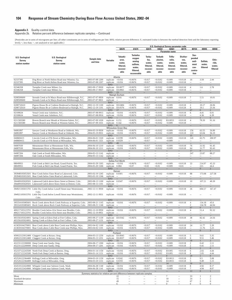
104 Response of Stream Chemistry During Base Flow Across United States, 2002–04
Appendix 2. Quality-control data. Appendix 2b. Relative percent difference between replicate samples.—Continued
[Pesticides are in units of micrograms per liter; all other constituents are in units of milligrams per liter. RPD, relative percent difference; E, estimated (value is between the method detection limit and the laboratory reporting level); <, less than; --, not analyzed or not applicable.]
U.S. Geological Survey
station number
U.S. Geological Survey
station name
Sample date and time
Variable
U.S. Geological Survey parameter code82670 61674 82675 04022 82661 38775 80154 00945 00940
Parameter name
Tebuthiuron,
water, filtered, recover
able
Terbufos oxygen analog
sulfone, water,
filtered, recoverable
Terbufos,
water, filtered, recover
able
Terbuthylazine, water,
filtered, recover
able
Trifluralin, water,
filtered, recover
able
Dichlorvos,
water, filtered,
recoverable
Suspended
sediment con
centration
Sulfate, water, filtered
Chloride,
water, filtered
Atlanta02337395 Dog River at North Helton Road near Winston, Ga. 2003-07-08 1200 replicate <0.016 <0.0676 <0.017 <0.0102 <0.009 <0.0118 16 3.59 2.4402337395 Dog River at North Helton Road near Winston, Ga. 2003-07-08 1207 replicate <0.016 <0.0676 <0.017 <0.0102 <0.009 <0.0118 -- -- --
RPD -- -- -- -- -- -- -- -- --02346358 Turnpike Creek near Milner, Ga. 2003-09-17 0930 replicate E0.0077 <0.0676 <0.017 <0.0102 <0.009 <0.0118 4 1.6 2.7802346358 Turnpike Creek near Milner, Ga. 2003-09-17 0937 replicate E0.0061 <0.0676 <0.017 <0.0102 <0.009 <0.0118 -- -- --
RPD 23 -- -- -- -- -- -- -- --Raleigh-Durham
0208500600 Strouds Creek at St Marys Road near Hillsborough, N.C. 2003-07-07 0830 replicate 0.016 <0.0676 <0.017 <0.0102 <0.009 <0.0118 7 5.51 10.010208500600 Strouds Creek at St Marys Road near Hillsborough, N.C. 2003-07-07 0831 replicate -- -- -- -- -- -- -- -- --
RPD -- -- -- -- -- -- -- -- --0208732610 Pigeon House Br at Crabtree Boulevard at Raleigh, N.C. 2002-12-19 1100 replicate E0.0484 <0.0676 <0.017 <0.0102 <0.009 <0.0118 2 19.17 26.060208732610 Pigeon House Br at Crabtree Boulevard at Raleigh, N.C. 2002-12-19 1101 replicate E0.0576 <0.0676 <0.017 <0.0102 <0.009 <0.0118 4 19.1 25.56
RPD 17 -- -- -- -- -- 67 0 202100634 Vestal Creek near Asheboro, N.C. 2003-07-08 0915 replicate <0.016 <0.0676 <0.017 <0.0102 <0.009 <0.0118 6 4.41 6.0102100634 Vestal Creek near Asheboro, N.C. 2003-07-08 0916 replicate <0.016 <0.0676 <0.017 <0.0102 <0.009 <0.0118 -- 4.36 6.39
RPD -- -- -- -- -- -- -- 1 60211583580 Bowen Branch near Mouth at Winston-Salem, N.C. 2003-07-09 1030 replicate 0.151 <0.0676 <0.017 <0.0102 E0.0053 <0.0118 4 78.39 91.160211583580 Bowen Branch near Mouth at Winston-Salem, N.C. 2003-07-09 1031 replicate 0.142 <0.0676 <0.017 <0.0102 <0.009 <0.0118 -- -- --
RPD 6 -- -- -- -- -- -- -- --Milwaukee-Green Bay
04081897 Sawyer Creek at Westhaven Road at Oshkosh, Wis. 2004-05-19 0930 replicate <0.016 <0.0676 <0.017 <0.0102 <0.009 <0.0118 156 63.55 56.8904081897 Sawyer Creek at Westhaven Road at Oshkosh, Wis. 2004-05-19 0931 replicate <0.016 <0.0676 <0.017 <0.0102 <0.009 <0.0118 110 63.04 56.19
RPD -- -- -- -- -- -- 35 1 1040869415 Lincoln Creek at 47th Street at Milwaukee, Wis. 2004-06-01 1320 replicate 0.0199 <0.0676 <0.017 <0.0102 <0.009 <0.0118 145 63.75 200.97040869415 Lincoln Creek at 47th Street at Milwaukee, Wis. 2004-06-01 1321 replicate 0.0329 -- <0.017 -- <0.009 -- -- -- --
RPD 49 -- -- -- -- -- -- -- --04087030 Menomonee River at Menomonee Falls, Wis. 2004-06-10 1210 replicate <0.016 <0.0676 <0.017 <0.0102 <0.009 <0.0118 76 31.92 91.4504087030 Menomonee River at Menomonee Falls, Wis. 2004-06-10 1211 replicate <0.016 <0.0676 <0.017 <0.0102 <0.009 <0.0118 64 31.77 92.43
RPD -- -- -- -- -- -- 17 0 104087204 Oak Creek at South Milwaukee, Wis. 2004-05-13 1141 replicate -- -- -- -- -- -- 247 23.87 88.2704087204 Oak Creek at South Milwaukee, Wis. 2004-05-13 1142 replicate -- -- -- -- -- -- -- -- --
RPD -- -- -- -- -- -- -- -- --Dallas-Fort Worth
08049955 Fish Creek at Belt Line Road, Grand Prairie, Tex. 2004-05-20 1505 replicate <0.016 <0.0676 <0.017 <0.0102 <0.009 <0.0118 33 214.97 45.3308049955 Fish Creek at Belt Line Road, Grand Prairie, Tex. 2004-05-20 1506 replicate 0.084 <0.07 <0.02 <0.01 <0.009 <0.01 -- 215 44.4
RPD -- -- -- -- -- -- -- 0 2Denver
393948105053501 Bear Creek below Estes Road at Lakewood, Colo. 2003-02-10 1245 replicate 0.0301 <0.0676 <0.017 <0.0102 <0.009 <0.0118 88 173.08 227.58393948105053501 Bear Creek below Estes Road at Lakewood, Colo. 2003-02-10 1246 replicate -- -- -- -- -- -- -- -- --
RPD -- -- -- -- -- -- -- -- --394409105020501 Lakewood Gulch above Knox Street at Denver, Colo. 2003-08-13 1100 replicate 0.0347 <0.0676 <0.017 <0.0102 <0.009 <0.0118 10 107.21 49.39394409105020501 Lakewood Gulch above Knox Street at Denver, Colo. 2003-08-13 1101 replicate -- -- -- -- -- -- -- -- --
RPD -- -- -- -- -- -- -- -- --394921105015701 Little Dry Creek below Lowell Street near Westminster,
Colo.2002-12-11 0930 replicate <0.016 <0.0676 <0.017 <0.0102 <0.009 <0.0118 26 694.57 167.47
394921105015701 Little Dry Creek below Lowell Street near Westminster, Colo.
2002-12-11 0931 replicate <0.016 <0.0676 <0.017 <0.0102 <0.009 <0.0118 -- -- --
RPD -- -- -- -- -- -- -- -- --395554105085601 Rock Creek above Rock Creek Parkway at Superior, Colo. 2003-08-21 1145 replicate <0.016 <0.0676 <0.017 <0.0102 <0.009 <0.0118 4 134.18 45.6395554105085601 Rock Creek above Rock Creek Parkway at Superior, Colo. 2003-08-21 1146 replicate -- -- -- -- -- -- 2 134.78 44.94
RPD -- -- -- -- -- -- 67 0 1400217105123701 Boulder Creek below 61st Street near Boulder, Colo. 2002-12-10 0950 replicate <0.016 <0.0676 <0.017 <0.0102 <0.009 <0.0118 4 51.4 92.32400217105123701 Boulder Creek below 61st Street near Boulder, Colo. 2002-12-10 0951 replicate -- -- -- -- -- -- -- -- --
RPD -- -- -- -- -- -- -- -- --403356105024001 Spring Creek at Edora Park at Fort Collins, Colo. 2003-08-27 1130 replicate E0.0342 <0.0676 <0.017 <0.0102 <0.009 <0.0118 38 82.42 24.56403356105024001 Spring Creek at Edora Park at Fort Collins, Colo. 2003-08-27 1131 replicate -- -- -- -- -- -- -- -- --
RPD -- -- -- -- -- -- -- -- --413659104370001 Bear Creek above Little Bear Creek near Phillips, Wyo. 2003-04-02 1100 replicate <0.016 <0.0676 <0.017 <0.0102 <0.009 <0.0118 24 11.77 5.39413659104370001 Bear Creek above Little Bear Creek near Phillips, Wyo. 2003-04-02 1101 replicate <0.016 <0.0676 <0.017 <0.0102 <0.009 <0.0118 -- 11.76 5.23
RPD -- -- -- -- -- -- -- 0 3Portland
450022123012400 Claggett Creek at Keizer, Oreg. 2004-05-13 1250 replicate E0.0043 <0.0676 <0.017 <0.0102 <0.009 <0.0118 5 9.61 5.35450022123012400 Claggett Creek at Keizer, Oreg. 2004-05-13 1251 replicate E0.0037 <0.0676 <0.017 <0.0102 <0.009 <0.0118 6 9.51 5.46
RPD 15 -- -- -- -- -- 18 1 2452231122200000 Deep Creek near Sandy, Oreg. 2004-08-17 1200 replicate <0.016 <0.0676 <0.017 <0.0102 <0.009 <0.0118 2 0.42 2.11452231122200000 Deep Creek near Sandy, Oreg. 2004-08-17 1201 replicate <0.016 <0.0676 <0.017 <0.0102 <0.009 <0.0118 2 0.41 2.11
RPD -- -- -- -- -- -- 0 2 0452337122243500 North Fork Deep Creek at Barton, Oreg. 2004-01-14 1150 replicate <0.016 <0.0676 <0.017 <0.0102 E0.005 <0.0118 6 2.02 4.44452337122243500 North Fork Deep Creek at Barton, Oreg. 2004-01-14 1151 replicate <0.016 <0.0676 <0.017 <0.0102 E0.005 <0.0118 8 2.05 4.44
RPD -- -- -- -- 0 -- 29 1 0452526122364400 Kellogg Creek at Milwaukie, Oreg. 2004-03-10 1150 replicate 0.0242 <0.0676 <0.017 <0.0102 E0.0013 <0.0118 3 9.5 5.08452526122364400 Kellogg Creek at Milwaukie, Oreg. 2004-03-10 1151 replicate 0.0193 <0.0676 <0.017 <0.0102 E0.0015 <0.0118 5 9.49 5.15
RPD 23 -- -- -- 14 -- 50 0 1454510122424900 Whipple Creek near Salmon Creek, Wash. 2004-06-28 1140 replicate <0.016 <0.0676 <0.017 <0.0102 <0.009 <0.0118 8 4.92 8.17454510122424900 Whipple Creek near Salmon Creek, Wash. 2004-06-28 1141 replicate <0.016 <0.0676 <0.017 <0.0102 <0.009 <0.0118 7 4.94 8.07
RPD -- -- -- -- -- -- 13 0 1Summary statistics for relative percent difference between replicate samples
Mean 22 -- -- -- 7 -- 33 1 2Standard deviation 15 -- -- -- 10 -- 24 1 2Maximum 49 -- -- -- 14 -- 67 2 6Minimum 6 -- -- -- 0 -- 0 0 0


106 Response of Stream Chemistry During Base Flow Across United States, 2002–04
Appendix 2. Quality-control data. Appendix 2c. Percent recovery of spiked pesticide compounds.
[All spike and environmental samples are in units of micrograms per liter. E, estimated (value is between the method detection limit and the laboratory reporting level); <, less than; M, presence of material verified, but not quantified; --, not analyzed or not applicable.]
U.S. Geological Survey station
number
U.S. Geological Survey
station name
Sample date and time
Variable
U.S. Geological Survey parameter code49295 82660 61615 61618 04040
Parameter name
1-Naphthol, water,
filtered, recoverable
2,6-Diethyl-aniline, water,
filtered, recoverable
2-[(2-Ethyl-6-methylphe-nyl)-amino]-1-propanol,
water, filtered, recoverable
2-Chloro-2’,6’-diethylacet-anilide, wa-ter, filtered, recoverable
2-Chloro-4-isopropyl-
amino-6-ami-no-s-triazine,
water, filtered,
recoverable
Atlanta02338523 Hillabahatchee Creek at Thaxton Road near Franklin, Ga. 2003-07-15 1516 spike E 0.105 0.111 <0.1256 0.129 E 0.073902338523 Hillabahatchee Creek at Thaxton Road near Franklin, Ga. 2003-07-15 1515 environmental <0.0882 <0.006 <0.1256 <0.005 <0.006
percent recovery 92 97 -- 112 6402335870 Sope Creek near Marietta, Ga. 2003-09-09 1131 spike -- 0.12 -- -- E 0.052902335870 Sope Creek near Marietta, Ga. 2003-09-09 1141 spike E 0.0158 -- 0.138 0.12 --02335870 Sope Creek near Marietta, Ga. 2003-09-09 1130 environmental <0.0882 <0.006 <0.1256 <0.005 E 0.003
percent recovery 14 105 120 105 4402334885 Suwanee Creek at Suwanee, Ga. 2003-07-08 1531 spike E 0.0235 0.107 E 0.154 0.126 E 0.052402334885 Suwanee Creek at Suwanee, Ga. 2003-07-08 1530 environmental <0.0882 <0.006 <0.1256 <0.005 <0.006
percent recovery 20 93 134 110 4602344797 White Oak Creek at Cannon Road near Raymond, Ga. 2003-07-15 1301 spike E 0.0772 0.112 0.131 0.126 E 0.067602344797 White Oak Creek at Cannon Road near Raymond, Ga. 2003-07-15 1300 environmental E 0.0116 <0.006 <0.1256 <0.005 E 0.0052
percent recovery 57 98 114 110 54Raleigh-Durham
0208725055 Black Creek at Weston Parkway near Cary, N.C. 2003-08-25 1301 spike E 0.0148 0.108 0.178 0.122 E 0.06120208725055 Black Creek at Weston Parkway near Cary, N.C. 2003-08-25 1300 environmental <0.0882 <0.006 <0.1256 <0.005 <0.006
percent recovery 13 94 155 106 5302085430 Deep Creek near Moriah, N.C. 2003-07-16 0905 spike E 0.0488 0.101 0.368 0.121 E 0.065102085430 Deep Creek near Moriah, N.C. 2003-07-16 0900 environmental <0.0882 <0.006 <0.31 <0.005 E 0.0181
percent recovery 43 88 321 106 4102097464 Morgan Creek near White Cross, N.C. 2003-07-15 1205 spike E 0.0471 0.101 E 0.123 0.106 E 0.075902097464 Morgan Creek near White Cross, N.C. 2003-07-15 1200 environmental <0.0882 <0.006 <0.1256 <0.005 E 0.0291
percent recovery 41 88 107 92 4102087580 Swift Creek near Apex, N.C. 2003-08-25 1003 spike -- 0.106 -- -- E 0.03202087580 Swift Creek near Apex, N.C. 2003-08-25 1004 spike E 0.0339 -- 0.172 0.121 --02087580 Swift Creek near Apex, N.C. 2003-08-25 1005 spike -- -- -- -- E 0.035902087580 Swift Creek near Apex, N.C. 2003-08-25 1000 environmental <0.0882 <0.006 <0.1256 <0.005 <0.006
percent recovery 30 92 150 106 31Milwaukee-Green Bay
040869415 Lincoln Creek at 47th Street at Milwaukee, Wis. 2004-02-03 1321 spike -- 0.0749 -- -- E 0.043040869415 Lincoln Creek at 47th Street at Milwaukee, Wis. 2004-02-03 1320 environmental -- <0.006 -- <0.005 <0.006
percent recovery -- 65 -- -- 37Dallas-Fort Worth
08063555 South Fork Chambers Creek near Creek 102 near Maypearl, Tex. 2004-03-31 1002 spike E 0.01 0.1 -- 0.12 E 0.15408063555 South Fork Chambers Creek near Creek 102 near Maypearl, Tex. 2004-03-31 1000 environmental <0.0882 <0.006 -- <0.005 E 0.1
percent recovery 9 87 -- 105 47Denver
400217105123701 Boulder Creek below 61st Street near Boulder, Colo. 2003-08-14 1122 spike E 0.0256 0.1 E 0.0912 0.118 E 0.0541400217105123701 Boulder Creek below 61st Street near Boulder, Colo. 2003-08-14 1120 environmental <0.0882 <0.006 <0.1256 <0.005 <0.006
percent recovery 22 87 80 103 47394409105020501 Lakewood Gulch above Knox Street at Denver, Colo. 2002-12-09 1222 spike E 0.0236 0.096 E 0.0988 0.112 E 0.0803394409105020501 Lakewood Gulch above Knox Street at Denver, Colo. 2002-12-09 1220 environmental E 0.0094 <0.006 <0.126 <0.005 <0.0063
percent recovery 12 84 86 98 70Portland
450022123012400 Claggett Creek at Keizer, Oreg. 2004-05-13 1253 spike E 0.0234 0.09 -- 0.116 E 0.0494450022123012400 Claggett Creek at Keizer, Oreg. 2004-05-13 1250 environmental <0.0882 <0.006 -- <0.005 E 0.0096
percent recovery 20 78 -- 101 35452231122200000 Deep Creek near Sandy, Oreg. 2004-08-17 1203 spike E 0.021 0.109 -- 0.117 E 0.0551452231122200000 Deep Creek near Sandy, Oreg. 2004-08-17 1200 environmental <0.0882 <0.006 -- <0.005 E 0.001
percent recovery 18 95 -- 102 4714206950 Fanno Creek at Durham, Oreg. 2004-04-29 1023 spike -- -- -- 0.106 --14206950 Fanno Creek at Durham, Oreg. 2004-04-29 1020 environmental -- <0.006 -- <0.005 E 0.0061
percent recovery -- -- -- 92 --452526122364400 Kellogg Creek at Milwaukie, Oreg. 2004-03-10 1153 spike E 0.0211 0.0947 -- 0.118 E 0.0559452526122364400 Kellogg Creek at Milwaukie, Oreg. 2004-03-10 1150 environmental <0.0882 <0.006 -- <0.005 E 0.005
percent recovery 18 83 -- 103 44452337122243500 North Fork Deep Creek at Barton, Oreg. 2004-01-14 1153 spike E 0.023 0.0989 E 0.0916 0.104 E 0.0533452337122243500 North Fork Deep Creek at Barton, Oreg. 2004-01-14 1150 environmental <0.0882 <0.006 <0.1256 <0.005 E 0.004
percent recovery 20 86 80 91 43454510122424900 Whipple Creek near Salmon Creek, Wa 2004-06-28 1143 spike E 0.0091 0.102 -- 0.116 E 0.0467454510122424900 Whipple Creek near Salmon Creek, Wa 2004-06-28 1140 environmental <0.0882 <0.006 -- <0.005 <0.006
percent recovery 8 89 -- 101 41Summary statistics for percent reovery of spiked compounds
Mean percent recovery 27 89 135 102 46Standard deviation of percent recovery 22 9 71 6 10Maximum percent recovery 92 105 321 112 70Minimum percent recovery 8 65 80 91 31Number of times compound was not detected in spike 0 0 1 0 0

Appendix 2. Quality-control data. Appendix 2c. Percent recovery of spiked pesticide compounds.—Continued
[All spike and environmental samples are in units of micrograms per liter. E, estimated (value is between the method detection limit and the laboratory reporting level); <, less than; M, presence of material verified, but not quantified; --, not analyzed or not applicable.]
U.S. Geological Survey parameter code61620 61625 61633 49260 46342 39632 61635 82686 82673 82680 61636
Parameter name
2-Ethyl-6-methylaniline,
water, filtered,
recoverable
3,4-Dichloroani-line, water,
filtered, recoverable
4-Chloro-2-methylphenol, water, filtered,
recoverable
Acetochlor, water, filtered,
recoverable
Alachlor, water, filtered,
recoverable
Atrazine, water, filtered,
recoverable
Azinphos-methyl oxygen analog, water,
filtered, recoverable
Azinphos-methyl, water,
filtered, recoverable
Benfluralin, water, filtered,
recoverable
Carbaryl, water, filtered,
recoverable
Chlorpyrifos oxygen analog, water,
filtered, recoverable
AtlantaE 0.103 0.0871 E 0.0787 0.136 0.101 0.135 E 0.0861 E 0.121 0.102 E 0.124 E 0.0769<0.0045 <0.0045 <0.0056 <0.006 <0.0045 <0.007 <0.016 <0.05 <0.01 <0.041 <0.056290 76 69 119 88 118 75 106 89 108 67
-- -- -- 0.123 0.116 0.117 -- E 0.142 0.1 E 0.144 --E 0.112 0.0841 E 0.0597 -- -- -- E 0.0629 -- -- -- E 0.0384<0.0045 <0.0045 <0.0056 <0.006 <0.0045 E 0.0048 <0.016 <0.05 <0.01 E 0.005 <0.056298 73 52 107 101 98 55 124 87 121 33
E 0.101 0.0696 E 0.0537 0.131 0.124 0.133 E 0.0805 E 0.125 0.102 E 0.146 E 0.0924<0.0045 <0.0045 <0.0056 <0.006 <0.0045 E 0.004 <0.125 <0.05 <0.01 E 0.0281 <0.056288 61 47 114 108 112 70 109 89 103 81
E 0.104 0.0769 E 0.0744 0.139 0.1 0.163 E 0.101 E 0.13 0.108 E 0.168 E 0.0857<0.0045 <0.0045 E 0.0015 <0.006 <0.0045 0.0314 <0.016 <0.05 <0.01 E 0.0284 <0.056291 67 64 121 87 115 88 113 94 122 75
Raleigh-DurhamE 0.104 0.0756 E 0.0616 0.124 0.119 0.126 E 0.0902 E 0.12 0.0887 E 0.1 E 0.0326<0.0045 <0.0045 <0.0056 <0.006 <0.0045 <0.007 <0.016 <0.05 <0.01 <0.041 <0.056291 66 54 108 104 110 79 105 77 87 28
E 0.0984 0.0651 E 0.0549 0.125 0.141 0.172 E 0.0986 E 0.123 0.102 E 0.162 E 0.0837<0.0045 <0.0045 <0.0056 <0.006 <0.0045 0.0505 <0.016 <0.05 <0.01 <0.041 <0.056286 57 48 109 123 106 86 107 89 141 73
E 0.101 0.0755 E 0.0496 0.119 0.12 0.254 E 0.0858 E 0.128 0.0888 E 0.118 E 0.0818<0.0045 <0.0045 <0.0056 <0.006 <0.0045 0.143 <0.016 <0.05 <0.01 <0.041 <0.056288 66 43 104 105 97 75 112 77 103 71
-- -- -- 0.126 0.13 0.0957 -- E 0.191 0.082 E 0.111 --E 0.104 0.0727 E 0.0532 -- -- -- E 0.0732 -- -- -- E 0.0797
-- -- -- -- -- E 0.0728 -- -- -- -- --<0.0045 0.0078 <0.0056 <0.006 <0.0045 E 0.0064 <0.016 <0.05 <0.01 <0.041 <0.056291 57 46 110 113 58 64 167 72 97 69
Milwaukee-Green Bay-- -- -- 0.13 0.129 0.148 -- E 0.182 0.12 E 0.23 --
<0.0045 <0.0045 <0.0056 <0.006 <0.005 0.0222 <0.016 <0.05 <0.01 <0.041 <0.0562-- -- -- 113 112 110 -- 159 105 201 --
Dallas-Fort WorthE 0.101 0.089 E 0.059 0.125 0.151 0.807 E 0.07 E 0.1 0.088 E 0.11 E 0.07<0.0045 0.0061 <0.0056 <0.006 0.0294 0.675 <0.016 <0.05 <0.01 E 0.0028 <0.056288 72 51 109 106 115 61 87 77 93 61
DenverE 0.102 0.0697 E 0.0554 0.123 0.121 0.127 E 0.0775 E 0.114 0.0824 E 0.1 E 0.0621<0.0045 <0.0045 <0.0056 <0.006 <0.0045 <0.007 <0.016 <0.05 <0.01 <0.041 <0.056289 61 48 107 106 111 68 99 72 87 54
E 0.0819 0.0779 E 0.0736 0.117 0.141 0.117 E 0.0986 E 0.154 0.0787 E 0.182 E 0.0421<0.0045 <0.0045 <0.0056 <0.006 <0.0045 0.0104 <0.016 <0.05 <0.01 E 0.0597 <0.056271 68 64 102 123 93 86 134 69 107 37
PortlandE 0.0878 0.0742 E 0.0461 0.121 0.116 0.136 E 0.0785 E 0.101 0.108 E 0.144 E 0.0896<0.0045 0.0227 <0.0056 <0.006 <0.005 0.0177 <0.016 <0.05 <0.01 E 0.0096 <0.056277 45 40 106 101 103 68 88 94 117 78
E 0.111 0.0694 E 0.0653 0.111 0.11 0.122 E 0.0533 E 0.094 0.0742 E 0.097 E 0.0137<0.0045 <0.0045 <0.0057 <0.006 <0.005 <0.007 <0.07 <0.05 <0.01 <0.041 <0.056297 61 57 97 96 106 46 82 65 85 12
E 0.102 0.0692 E 0.0424 -- -- -- E 0.0948 -- -- -- E 0.0608<0.0045 0.0056 <0.0056 <0.006 <0.005 0.0124 <0.016 <0.05 <0.01 E 0.0499 <0.056289 55 37 -- -- -- 83 -- -- -- 53
E 0.088 0.0727 E 0.0558 0.117 0.112 0.119 E 0.112 E 0.123 0.0878 E 0.19 E 0.0879<0.0045 E 0.002 <0.0056 <0.006 <0.005 E 0.0027 <0.016 <0.05 <0.01 E 0.0232 <0.056277 62 49 102 98 101 98 107 77 145 77
E 0.0928 0.124 E 0.0536 0.0891 0.0962 0.146 E 0.096 E 0.101 0.075 E 0.174 E 0.0559<0.0045 0.0613 <0.0056 <0.006 <0.005 0.0297 <0.031 <0.05 <0.01 E 0.0068 <0.056281 55 47 78 84 101 84 88 65 146 49
E 0.0968 0.0661 E 0.0506 0.114 0.113 0.117 E 0.147 E 0.13 0.0821 E 0.119 E 0.0644<0.0045 <0.0045 <0.0056 <0.006 <0.005 <0.007 <0.016 <0.05 <0.01 <0.041 <0.056284 58 44 99 99 102 128 113 72 104 56
Summary statistics for percent reovery of spiked compounds87 62 51 106 103 103 77 112 81 116 57
7 8 9 10 11 14 19 23 12 29 2098 76 69 121 123 118 128 167 105 201 8171 45 37 78 84 58 46 82 65 85 12
0 0 0 0 0 0 0 0 0 0 0
Appendix 2. Quality-control data 107

108 Response of Stream Chemistry During Base Flow Across United States, 2002–04
Appendix 2. Quality-control data. Appendix 2c. Percent recovery of spiked pesticide compounds.— Continued
[All spike and environmental samples are in units of micrograms per liter. E, estimated (value is between the method detection limit and the laboratory reporting level); <, less than; M, presence of material veri-fied, but not quantified; --, not analyzed or not applicable.]
U.S. Geological Survey
station numberU.S. Geological Survey
station name
Sample date and time
Variable
U.S. Geological Survey parameter code38933 82687 61585 61586 82682
Parameter name
Chlorpyrifos, water,
filtered, recoverable
cis-Perme-thrin, water,
filtered, recoverable
Cyfluthrin, water,
filtered, recoverable
Cypermethrin, water,
filtered, recoverable
DCPA, water,
filtered, recoverable
Atlanta02338523 Hillabahatchee Creek at Thaxton Road near Franklin, Ga. 2003-07-15 1516 spike 0.123 0.0833 E 0.0776 E 0.0768 0.12802338523 Hillabahatchee Creek at Thaxton Road near Franklin, Ga. 2003-07-15 1515 environmental <0.005 <0.006 <0.008 <0.0086 <0.003
percent recovery 107 73 68 67 11202335870 Sope Creek near Marietta, Ga. 2003-09-09 1131 spike 0.109 0.0743 -- -- 0.107
02335870 Sope Creek near Marietta, Ga. 2003-09-09 1141 spike -- -- E 0.0817 E 0.0776 --02335870 Sope Creek near Marietta, Ga. 2003-09-09 1130 environmental <0.005 <0.006 <0.008 <0.0086 <0.003
percent recovery 95 65 71 68 9302334885 Suwanee Creek at Suwanee, Ga. 2003-07-08 1531 spike 0.122 0.0912 E 0.0846 E 0.0848 0.12702334885 Suwanee Creek at Suwanee, Ga. 2003-07-08 1530 environmental <0.005 <0.006 <0.008 <0.0086 <0.003
percent recovery 106 80 74 74 11102344797 White Oak Creek at Cannon Road near Raymond, Ga. 2003-07-15 1301 spike 0.128 0.0832 E 0.082 E 0.0796 0.12502344797 White Oak Creek at Cannon Road near Raymond, Ga. 2003-07-15 1300 environmental <0.005 <0.006 <0.008 <0.0086 <0.003
percent recovery 112 73 72 69 109Raleigh-Durham
0208725055 Black Creek at Weston Parkway near Cary, N.C. 2003-08-25 1301 spike 0.11 0.0944 E 0.0829 E 0.0812 0.1170208725055 Black Creek at Weston Parkway near Cary, N.C. 2003-08-25 1300 environmental <0.005 <0.006 <0.008 <0.0086 <0.003
percent recovery 96 82 72 71 10202085430 Deep Creek near Moriah, N.C. 2003-07-16 0905 spike 0.122 0.0812 E 0.0958 E 0.0795 0.1202085430 Deep Creek near Moriah, N.C. 2003-07-16 0900 environmental <0.005 <0.006 <0.008 <0.0086 <0.003
percent recovery 106 71 84 69 10502097464 Morgan Creek near White Cross, N.C. 2003-07-15 1205 spike 0.115 0.0793 E 0.0818 E 0.0852 0.12102097464 Morgan Creek near White Cross, N.C. 2003-07-15 1200 environmental <0.005 <0.006 <0.008 <0.0086 <0.003
percent recovery 100 69 71 74 10602087580 Swift Creek near Apex, N.C. 2003-08-25 1003 spike 0.0975 0.0619 -- -- 0.098902087580 Swift Creek near Apex, N.C. 2003-08-25 1004 spike -- -- E 0.0683 E 0.0668 --02087580 Swift Creek near Apex, N.C. 2003-08-25 1005 spike -- -- -- -- --02087580 Swift Creek near Apex, N.C. 2003-08-25 1000 environmental <0.005 <0.006 <0.008 <0.0086 <0.003
percent recovery 85 54 60 58 86Milwaukee-Green Bay
040869415 Lincoln Creek at 47th Street at Milwaukee, Wis. 2004-02-03 1321 spike 0.149 0.0674 -- -- 0.119040869415 Lincoln Creek at 47th Street at Milwaukee, Wis. 2004-02-03 1320 environmental <0.005 <0.006 <0.008 <0.0086 <0.003
percent recovery 130 59 -- -- 104Dallas-Fort Worth
08063555 South Fork Chambers Creek near Creek 102 near Maypearl, Tex. 2004-03-31 1002 spike 0.113 0.053 E 0.062 E 0.063 0.11608063555 South Fork Chambers Creek near Creek 102 near Maypearl, Tex. 2004-03-31 1000 environmental <0.005 <0.006 <0.008 <0.0086 <0.003
percent recovery 99 46 54 55 101Denver
400217105123701 Boulder Creek below 61st Street near Boulder, Colo. 2003-08-14 1122 spike 0.111 0.0832 E 0.0695 E 0.0653 0.121400217105123701 Boulder Creek below 61st Street near Boulder, Colo. 2003-08-14 1120 environmental <0.005 <0.006 <0.008 <0.0086 <0.003
percent recovery 97 73 61 57 106394409105020501 Lakewood Gulch above Knox Street at Denver, Colo. 2002-12-09 1222 spike 0.108 E 0.0796 E 0.103 E 0.0924 0.122394409105020501 Lakewood Gulch above Knox Street at Denver, Colo. 2002-12-09 1220 environmental <0.005 <0.006 <0.008 <0.0086 <0.003
percent recovery 94 69 90 81 106Portland
450022123012400 Claggett Creek at Keizer, Oreg. 2004-05-13 1253 spike 0.116 0.0574 E 0.0762 E 0.0735 0.119450022123012400 Claggett Creek at Keizer, Oreg. 2004-05-13 1250 environmental <0.005 <0.006 <0.008 <0.0086 <0.003
percent recovery 101 50 66 64 104452231122200000 Deep Creek near Sandy, Oreg. 2004-08-17 1203 spike 0.098 0.0636 E 0.0532 E 0.0533 0.116452231122200000 Deep Creek near Sandy, Oreg. 2004-08-17 1200 environmental <0.005 <0.006 <0.008 <0.0086 <0.003
percent recovery 85 55 46 46 10114206950 Fanno Creek at Durham, Oreg. 2004-04-29 1023 spike -- -- E 0.0754 E 0.0614 --14206950 Fanno Creek at Durham, Oreg. 2004-04-29 1020 environmental <0.005 <0.006 <0.008 <0.0086 <0.003
percent recovery -- -- 66 54 --452526122364400 Kellogg Creek at Milwaukie, Oreg. 2004-03-10 1153 spike 0.108 0.0778 E 0.0977 E 0.088 0.108452526122364400 Kellogg Creek at Milwaukie, Oreg. 2004-03-10 1150 environmental <0.005 <0.006 <0.008 <0.0086 <0.003
percent recovery 94 68 85 77 94452337122243500 North Fork Deep Creek at Barton, Oreg. 2004-01-14 1153 spike 0.123 0.0615 E 0.0713 E 0.0671 0.114452337122243500 North Fork Deep Creek at Barton, Oreg. 2004-01-14 1150 environmental 0.0134 <0.006 <0.008 <0.0086 <0.003
percent recovery 96 54 62 59 99454510122424900 Whipple Creek near Salmon Creek, Wa 2004-06-28 1143 spike 0.107 0.0734 E 0.1 E 0.0879 0.12454510122424900 Whipple Creek near Salmon Creek, Wa 2004-06-28 1140 environmental <0.005 <0.006 <0.03 <0.03 <0.003
percent recovery 93 64 87 77 105Summary statistics for percent reovery of spiked compounds
Mean percent recovery 100 65 70 66 103Standard deviation of percent recovery 11 10 12 10 6Maximum percent recovery 130 82 90 81 112Minimum percent recovery 85 46 46 46 86Number of times compound was not detected in spike 0 0 0 0 0

Appendix 2. Quality-control data. Appendix 2c. Percent recovery of spiked pesticide compounds.— Continued
[All spike and environmental samples are in units of micrograms per liter. E, estimated (value is between the method detection limit and the laboratory reporting level); <, less than; M, presence of material verified, but not quantified; --, not analyzed or not applicable.]
U.S. Geological Survey parameter code62170 61638 39572 38454 39381 82662 61644 82346 61645 61646 61591
Parameter name
Desulfinyl fipronil, water,
filtered, recoverable
Diazinon oxygen
analog, water, filtered,
recoverable
Diazinon, water,
filtered, recoverable
Dicrotophos, water,
filtered, recoverable
Dieldrin, water,
filtered, recoverable
Dimethoate, water,
filtered,recoverable
Ethion monox-on, water, filtered,
recoverable
Ethion, water,
filtered, recoverable
Fenamiphos sulfone, water,
filtered, recoverable
Fenamiphos sulfoxide,
water, filtered,
recoverable
Fenamiphos, water,
filtered, recoverable
Atlanta0.13 0.116 0.124 E 0.0728 0.0963 E 0.0422 E 0.124 0.12 0.117 E 0.108 0.111
<0.004 <0.01 <0.005 <0.0843 <0.0048 <0.0061 <0.0336 <0.004 <0.0077 <0.031 <0.029113 101 108 63 84 37 108 105 102 94 97
-- -- 0.111 -- 0.117 -- -- -- -- -- ---- -- -- E 0.0473 -- E 0.0298 E 0.096 0.0941 E 0.124 E 0.086 0.111
<0.004 -- <0.005 <0.0843 <0.0048 <0.0061 <0.0336 <0.004 <0.0077 <0.031 <0.029-- -- 97 41 102 26 84 82 108 75 97
0.112 0.111 0.125 E 0.046 0.117 E 0.0286 E 0.119 0.126 0.136 E 0.11 E 0.141<0.004 <0.01 0.0079 <0.0843 <0.0048 <0.0061 <0.0336 <0.004 <0.0077 <0.125 <0.02998 97 102 40 102 25 104 110 119 96 123
0.13 0.12 0.124 E 0.067 0.103 E 0.0294 E 0.14 0.13 0.143 E 0.167 0.154<0.004 <0.01 0.0055 <0.0843 <0.0048 <0.0061 <0.0336 <0.004 <0.0077 <0.031 <0.029
113 105 103 58 90 26 122 113 125 146 134Raleigh-Durham
0.122 0.0997 0.0992 E 0.0404 0.108 E 0.0293 E 0.11 0.128 E 0.123 E 0.107 E 0.101<0.004 <0.01 <0.005 <0.0843 <0.0048 <0.0061 <0.0336 <0.004 <0.0077 <0.031 <0.029
106 87 87 35 94 26 96 112 107 93 880.146 0.124 0.121 E 0.0439 0.103 E 0.0281 E 0.145 0.128 0.16 E 0.137 0.196
<0.004 <0.01 <0.005 <0.0843 <0.0048 <0.0061 <0.0336 <0.004 <0.0077 <0.031 <0.029127 108 106 38 90 25 126 112 140 119 171
0.12 0.103 0.114 E 0.0297 0.127 E 0.0266 E 0.116 0.119 0.125 E 0.0601 E 0.128<0.004 <0.01 <0.005 <0.0843 <0.0048 <0.0061 <0.0336 <0.004 <0.0077 <0.031 <0.029
105 90 99 26 111 23 101 104 109 52 1120.0077 -- 0.12 -- 0.139 -- -- -- -- -- --
-- -- -- E 0.0446 -- E 0.026 E 0.109 0.0999 0.13 E 0.0888 0.126-- -- -- -- -- -- -- -- -- -- --
0.006 -- E 0.0041 <0.0843 <0.0048 <0.0061 <0.0336 <0.004 <0.0077 <0.031 <0.0291 -- 101 39 121 23 95 87 113 77 110
Milwaukee-Green Bay0.149 -- 0.119 -- 0.109 -- -- -- -- -- --
<0.012 -- <0.005 <0.0843 <0.009 <0.0061 <0.0336 <0.004 <0.0077 <0.031 <0.029130 -- 104 -- 95 -- -- -- -- -- --
Dallas-Fort Worth0.118 0.11 0.113 E 0.03 0.104 E 0.029 E 0.11 0.104 0.136 E 0.05 0.14
<0.012 <0.01 <0.005 <0.0843 <0.009 <0.0061 <0.0336 <0.004 <0.0077 <0.031 <0.029103 96 99 26 91 25 96 91 119 44 122
Denver0.116 0.0969 0.11 E 0.0383 0.135 E 0.0261 E 0.108 0.124 0.0984 E 0.0712 0.12
<0.004 <0.01 <0.005 <0.0843 <0.0048 <0.0061 <0.0336 <0.004 <0.0077 <0.031 <0.029101 84 96 33 118 23 94 108 86 62 105
0.102 0.11 0.121 E 0.0456 0.103 E 0.0458 E 0.118 0.105 0.154 E 0.0976 0.144<0.004 <0.04 <0.005 <0.0843 <0.0048 <0.0061 <0.0336 <0.004 <0.0077 <0.031 <0.02989 96 106 40 90 40 103 92 134 85 126
Portland0.129 0.107 0.11 E 0.0388 0.0914 E 0.0242 E 0.112 0.108 0.137 E 0.103 0.149
<0.012 <0.01 <0.005 <0.0843 <0.009 <0.0061 <0.0336 <0.004 <0.0077 <0.031 <0.029112 93 96 34 80 21 98 94 119 90 130
0.111 0.0735 0.106 E 0.0259 0.134 E 0.0284 E 0.084 0.102 0.0731 E 0.0683 0.086<0.012 <0.006 <0.005 <0.0843 <0.009 <0.0061 <0.002 <0.004 <0.0491 <0.0387 <0.02997 64 92 23 117 25 73 89 64 60 75
-- -- -- E 0.0308 -- E 0.0232 E 0.0881 0.088 0.106 E 0.0746 0.0996<0.012 -- 0.008 <0.0843 <0.009 <0.0061 <0.0336 <0.004 <0.0077 <0.031 <0.029
-- -- -- 27 -- 20 77 77 92 65 870.112 0.1 0.102 E 0.0469 0.0972 E 0.0305 E 0.118 0.118 0.154 E 0.102 0.13
<0.012 <0.01 <0.005 <0.0843 <0.009 <0.0061 <0.0336 <0.004 <0.0077 <0.031 <0.02998 87 89 41 85 27 103 103 134 89 113
0.12 0.0922 0.0956 E 0.0336 0.0886 E 0.0229 E 0.0905 0.0852 0.134 E 0.106 0.111<0.012 <0.01 <0.005 <0.0843 E 0.0023 <0.0061 <0.0336 <0.004 <0.0077 <0.031 <0.029
105 80 83 29 75 20 79 74 117 92 970.123 0.0909 0.105 E 0.0424 0.113 E 0.0258 0.122 0.112 E 0.132 E 0.107 E 0.103
<0.012 <0.01 <0.005 <0.0843 <0.009 <0.0061 <0.0336 <0.004 <0.0077 <0.031 <0.029107 79 92 37 99 22 106 98 115 93 90
Summary statistics for percent reovery of spiked compounds100 91 98 37 97 25 98 97 112 84 110
28 11 7 11 14 5 14 13 19 25 23130 108 108 63 121 40 126 113 140 146 171
1 64 83 23 75 20 73 74 64 44 750 0 0 0 0 0 0 0 0 0 0
Appendix 2. Quality-control data 109

110 Response of Stream Chemistry During Base Flow Across United States, 2002–04
Appendix 2. Quality-control data. Appendix 2c. Percent recovery of spiked pesticide compounds.— Continued
[All spike and environmental samples are in units of micrograms per liter. E, estimated (value is between the method detection limit and the laboratory reporting level); <, less than; M, presence of material veri-fied, but not quantified; --, not analyzed or not applicable.]
U.S. Geological Survey
station number
U.S. Geological Survey station name
Sample date and time
Variable
U.S. Geological Survey parameter code62169 62167 62168 62166 61649
Parameter name
Desulfi-nylfipronil
amide, water,
filtered, recoverable
Fipronil sulfide, water,
filtered, recoverable
Fipronil sulfone, water,
filtered, recoverable
Fipronil, water,
filtered, recoverable
Fonofos oxygen analog, water,
filtered, recoverable
Atlanta02338523 Hillabahatchee Creek at Thaxton Road near Franklin, Ga. 2003-07-15 1516 spike E 0.154 0.136 0.113 E 0.144 E 0.11902338523 Hillabahatchee Creek at Thaxton Road near Franklin, Ga. 2003-07-15 1515 environmental <0.009 <0.005 <0.005 <0.007 <0.0021
percent recovery 134 119 99 126 10402335870 Sope Creek near Marietta, Ga. 2003-09-09 1131 spike -- -- E 0.0054 -- --
02335870 Sope Creek near Marietta, Ga. 2003-09-09 1141 spike -- -- -- -- E 0.10202335870 Sope Creek near Marietta, Ga. 2003-09-09 1130 environmental E 0.004 <0.005 <0.005 <0.007 <0.0021
percent recovery -- -- 5 -- 8902334885 Suwanee Creek at Suwanee, Ga. 2003-07-08 1531 spike E 0.139 0.119 0.11 E 0.124 E 0.10902334885 Suwanee Creek at Suwanee, Ga. 2003-07-08 1530 environmental <0.009 <0.005 <0.005 E 0.0069 <0.0021
percent recovery 121 104 96 102 9502344797 White Oak Creek at Cannon Road near Raymond, Ga. 2003-07-15 1301 spike E 0.173 0.139 0.127 E 0.181 E 0.11802344797 White Oak Creek at Cannon Road near Raymond, Ga. 2003-07-15 1300 environmental <0.009 <0.005 <0.005 <0.007 <0.0021
percent recovery 151 121 111 158 103Raleigh-Durham
0208725055 Black Creek at Weston Parkway near Cary, N.C. 2003-08-25 1301 spike E 0.158 0.137 0.126 0.113 E 0.1090208725055 Black Creek at Weston Parkway near Cary, N.C. 2003-08-25 1300 environmental <0.009 E 0.0079 <0.005 E 0.0158 <0.0021
percent recovery 138 113 110 85 9502085430 Deep Creek near Moriah, N.C. 2003-07-16 0905 spike E 0.163 0.144 0.128 E 0.162 E 0.11602085430 Deep Creek near Moriah, N.C. 2003-07-16 0900 environmental <0.009 <0.005 <0.005 <0.007 <0.0021
percent recovery 142 126 112 141 10102097464 Morgan Creek near White Cross, N.C. 2003-07-15 1205 spike E 0.134 0.124 0.109 E 0.132 E 0.085202097464 Morgan Creek near White Cross, N.C. 2003-07-15 1200 environmental <0.009 <0.005 <0.006 <0.007 <0.0021
percent recovery 117 108 95 115 7402087580 Swift Creek near Apex, N.C. 2003-08-25 1003 spike -- 0.0093 0.0089 E 0.0148 --02087580 Swift Creek near Apex, N.C. 2003-08-25 1004 spike -- -- -- -- E 0.11602087580 Swift Creek near Apex, N.C. 2003-08-25 1005 spike -- -- -- -- --02087580 Swift Creek near Apex, N.C. 2003-08-25 1000 environmental <0.009 0.007 0.009 E 0.0152 <0.0021
percent recovery -- -- -- -- 101Milwaukee-Green Bay
040869415 Lincoln Creek at 47th Street at Milwaukee, Wis. 2004-02-03 1321 spike E 0.181 0.137 0.138 E 0.225 --040869415 Lincoln Creek at 47th Street at Milwaukee, Wis. 2004-02-03 1320 environmental <0.029 <0.013 <0.024 <0.016 <0.0021
percent recovery 158 119 120 196 --Dallas-Fort Worth
08063555 South Fork Chambers Creek near Creek 102 near Maypearl, Tex. 2004-03-31 1002 spike E 0.128 0.122 0.098 E 0.151 E 0.10708063555 South Fork Chambers Creek near Creek 102 near Maypearl, Tex. 2004-03-31 1000 environmental <0.029 <0.013 <0.024 <0.016 <0.0021
percent recovery 112 106 85 132 93Denver
400217105123701 Boulder Creek below 61st Street near Boulder, Colo. 2003-08-14 1122 spike E 0.13 0.113 0.108 E 0.106 E 0.0895400217105123701 Boulder Creek below 61st Street near Boulder, Colo. 2003-08-14 1120 environmental <0.009 <0.005 <0.005 <0.007 <0.0021
percent recovery 113 99 94 92 78394409105020501 Lakewood Gulch above Knox Street at Denver, Colo. 2002-12-09 1222 spike 0.147 0.119 0.112 0.12 E 0.0944394409105020501 Lakewood Gulch above Knox Street at Denver, Colo. 2002-12-09 1220 environmental <0.009 <0.005 <0.005 <0.007 <0.0021
percent recovery 128 104 98 105 82Portland
450022123012400 Claggett Creek at Keizer, Oreg. 2004-05-13 1253 spike E 0.126 0.133 0.103 E 0.16 E 0.106450022123012400 Claggett Creek at Keizer, Oreg. 2004-05-13 1250 environmental <0.029 <0.013 <0.024 <0.016 <0.0021
percent recovery 110 116 90 140 92452231122200000 Deep Creek near Sandy, Oreg. 2004-08-17 1203 spike E 0.104 0.1 0.0972 E 0.0891 E 0.079452231122200000 Deep Creek near Sandy, Oreg. 2004-08-17 1200 environmental <0.029 <0.013 <0.024 <0.016 <0.0029
percent recovery 91 87 85 78 6914206950 Fanno Creek at Durham, Oreg. 2004-04-29 1023 spike -- -- -- -- E 0.088714206950 Fanno Creek at Durham, Oreg. 2004-04-29 1020 environmental <0.029 <0.013 <0.024 <0.016 <0.0021
percent recovery -- -- -- -- 77452526122364400 Kellogg Creek at Milwaukie, Oreg. 2004-03-10 1153 spike E 0.148 0.123 0.102 E 0.143 E 0.11452526122364400 Kellogg Creek at Milwaukie, Oreg. 2004-03-10 1150 environmental <0.029 <0.013 <0.024 <0.016 <0.0021
percent recovery 129 107 89 125 96452337122243500 North Fork Deep Creek at Barton, Oreg. 2004-01-14 1153 spike E 0.136 0.118 0.0968 E 0.124 E 0.0927452337122243500 North Fork Deep Creek at Barton, Oreg. 2004-01-14 1150 environmental <0.029 <0.013 <0.024 <0.016 <0.0021
percent recovery 119 103 84 108 81454510122424900 Whipple Creek near Salmon Creek, Wa 2004-06-28 1143 spike E 0.134 0.133 0.144 E 0.142 E 0.0914454510122424900 Whipple Creek near Salmon Creek, Wa 2004-06-28 1140 environmental <0.029 <0.013 <0.024 <0.016 <0.0021
percent recovery 117 116 126 124 80Summary statistics for percent reovery of spiked compounds
Mean percent recovery 125 110 94 122 89Standard deviation of percent recovery 17 10 27 30 11Maximum percent recovery 158 126 126 196 104Minimum percent recovery 91 87 5 78 69Number of times compound was not detected in spike 0 0 0 0 0

Appendix 2. Quality-control data. Appendix 2c. Percent recovery of spiked pesticide compounds.— Continued
[All spike and environmental samples are in units of micrograms per liter. E, estimated (value is between the method detection limit and the laboratory reporting level); <, less than; M, pres-ence of material verified, but not quantified; --, not analyzed or not applicable.]
U.S. Geological Survey parameter code04095 04025 61593 61594 61652 39532 61596 61598 61664 82667 39415 82630
Parameter name
Fonofos, water,
filtered, recoverable
Hexazinone, water,
filtered, recoverable
Iprodione, water,
filtered, recoverable
Isofenphos, water,
filtered, recoverable
Malaoxon, water,
filtered, recoverable
Malathion, water,
filtered, recoverable
Metalaxyl, water,
filtered, recoverable
Methidathion, water,
filtered, recoverable
Methyl paraoxon,
water, filtered,
recoverable
Methyl parathion,
water, filtered,
recoverable
Metolachlor, water,
filtered, recoverable
Metribuzin, water,
filtered, recoverable
Atlanta0.116 0.126 E 0.019 0.142 0.12 0.127 0.125 0.123 E 0.103 0.119 0.13 0.124
<0.0027 <0.0129 <1.4223 <0.0034 <0.008 <0.027 <0.0051 <0.0058 <0.0299 <0.006 <0.013 <0.006101 110 17 124 105 111 109 107 90 104 113 108
0.106 -- -- -- -- 0.13 -- -- -- 0.115 0.126 0.0938-- 0.105 <1.4223 0.103 0.102 -- 0.119 0.096 E 0.081 -- -- --
<0.0027 <0.0129 <1.4223 <0.0034 <0.008 <0.027 <0.0051 <0.0058 <0.0299 <0.006 <0.013 <0.00692 92 -- 90 89 113 104 84 71 100 110 820.111 0.123 E 0.0287 0.119 0.112 0.121 0.112 0.119 E 0.0952 0.11 0.128 0.102
<0.0027 <0.0129 <1.4223 <0.0034 <0.008 <0.027 <0.0051 <0.0058 <0.0299 <0.006 <0.013 <0.00697 107 25 104 98 106 98 104 83 96 112 890.119 0.137 E 0.0278 0.138 0.131 0.131 0.123 0.128 E 0.0969 0.126 0.13 0.118
<0.0027 <0.0129 <1.4223 <0.0034 <0.008 <0.027 <0.0051 <0.0058 <0.0299 <0.006 <0.013 <0.006104 119 24 120 114 114 107 112 84 110 113 103
Raleigh-Durham0.0951 0.126 E 0.0183 0.115 0.0836 0.104 0.116 0.112 E 0.0807 0.0704 0.121 0.0967
<0.0027 <0.0129 <1.4223 <0.0034 <0.008 <0.027 <0.0051 <0.0058 <0.0299 <0.006 <0.013 <0.00683 110 16 100 73 91 101 98 70 61 106 840.11 0.128 E 0.02 0.161 0.121 0.128 0.131 0.117 E 0.101 0.106 0.132 0.0961
<0.0027 <0.0129 <1.4223 <0.0034 <0.008 <0.027 <0.0051 <0.0058 <0.0299 <0.006 E 0.007 <0.00696 112 17 140 106 112 114 102 88 92 109 840.103 0.114 E 0.0304 0.116 0.105 0.114 0.111 0.111 E 0.0935 0.103 0.136 0.097
<0.0027 <0.0129 <1.4223 <0.0034 <0.008 <0.027 <0.0051 <0.0058 <0.0299 <0.006 0.0198 <0.00690 99 27 101 92 99 97 97 82 90 101 850.113 -- -- -- -- 0.107 -- -- -- 0.152 0.118 0.0825-- 0.103 E 0.022 0.0963 0.124 -- 0.117 0.107 E 0.104 -- -- ---- -- -- -- -- -- -- -- -- -- -- --
<0.0027 <0.0129 <1.4223 <0.0034 <0.008 <0.027 <0.0051 <0.0058 <0.0299 <0.006 E 0.0051 <0.00699 90 19 84 108 93 102 93 91 133 98 72
Milwaukee-Green Bay0.122 -- -- -- -- 0.176 -- -- -- 0.164 0.133 0.0735
<0.003 <0.0129 <1.4223 <0.0034 <0.008 <0.027 <0.0051 <0.0058 <0.0299 <0.015 <0.013 <0.006106 -- -- -- -- 153 -- -- -- 143 116 64
Dallas-Fort Worth0.104 0.113 M 0.134 0.096 0.101 0.129 0.108 E 0.09 0.107 0.141 0.097
<0.003 <0.0129 <1.4223 <0.0034 <0.008 <0.027 <0.0051 <0.0058 <0.0299 <0.015 0.0187 <0.00691 99 -- 117 84 88 112 94 78 93 107 85
Denver0.102 0.106 E 0.0224 0.119 0.0872 0.104 0.116 0.119 E 0.0763 0.0918 0.124 0.0933
<0.0027 <0.0129 <1.4223 <0.0034 <0.008 <0.027 <0.0051 <0.0058 <0.0299 <0.006 E 0.0057 <0.00689 92 20 104 76 91 101 104 67 80 103 810.0928 -- E 0.133 0.114 0.113 0.123 0.0925 0.118 E 0.0591 0.0974 0.127 0.105
<0.0027 -- E 0.0252 <0.0034 <0.008 <0.027 <0.0051 <0.0058 <0.0299 <0.006 <0.013 <0.00681 -- 94 99 99 107 81 103 52 85 111 92
Portland0.104 0.109 E 0.0586 0.128 0.127 0.114 0.123 0.103 E 0.107 0.128 0.123 0.0901
<0.003 <0.0129 <1.4223 <0.0034 <0.008 <0.027 <0.0051 <0.0058 <0.0299 <0.015 E 0.0049 <0.00691 95 51 112 111 99 107 90 93 112 103 790.101 0.102 E 0.0117 0.101 0.0684 0.0882 0.105 0.11 E 0.0612 0.0772 0.11 0.088
<0.003 0.0172 <0.387 <0.0034 <0.0298 <0.027 <0.0051 <0.0058 <0.0299 <0.015 <0.013 <0.00688 74 10 88 60 77 92 96 53 67 96 77
-- 0.0939 E 0.0222 0.0842 0.0871 -- 0.0978 0.0904 E 0.0651 -- -- --<0.003 <0.0129 <1.4223 <0.0034 <0.008 <0.027 <0.0051 <0.0058 <0.0299 <0.015 E 0.0082 <0.006
-- 82 19 73 76 -- 85 79 57 -- -- --0.0976 0.124 E 0.0392 0.127 0.105 0.111 0.115 0.118 E 0.0942 0.11 0.116 0.097
<0.003 <0.0129 <1.4223 <0.0034 <0.008 <0.027 <0.0051 <0.0058 <0.0299 <0.015 E 0.004 <0.00685 108 34 111 92 97 100 103 82 96 98 850.0921 0.117 E 0.0872 0.114 0.0976 0.104 0.114 0.0936 E 0.0758 0.0957 0.138 0.0858
<0.003 0.0159 <1.4223 <0.0034 <0.008 <0.027 E 0.0045 <0.0058 <0.0299 <0.015 0.0288 <0.00680 88 76 99 85 91 95 82 66 83 95 750.101 0.118 E 0.0348 0.128 0.101 0.111 0.126 0.093 E 0.083 0.0921 0.116 0.0901
<0.003 <0.0129 <1.4223 <0.0034 <0.008 <0.027 <0.0051 <0.0058 <0.0299 <0.015 <0.013 <0.00688 103 30 112 88 97 110 81 72 80 101 79
Summary statistics for percent reovery of spiked compounds92 99 32 105 91 102 101 96 75 96 105 848 12 24 16 15 17 9 10 13 21 7 11
106 119 94 140 114 153 114 112 93 143 116 10880 74 10 73 60 77 81 79 52 61 95 640 0 1 0 0 0 0 0 0 0 0 0
Appendix 2. Quality-control data 111
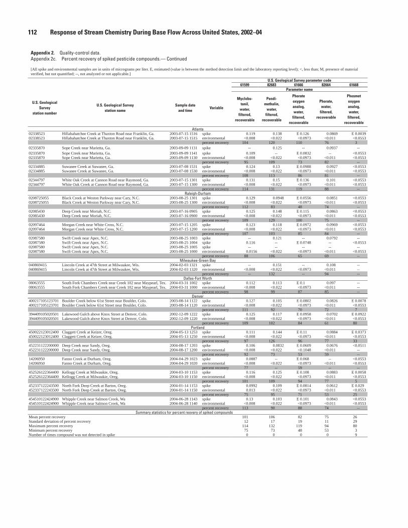
112 Response of Stream Chemistry During Base Flow Across United States, 2002–04
Appendix 2. Quality-control data. Appendix 2c. Percent recovery of spiked pesticide compounds.— Continued
[All spike and environmental samples are in units of micrograms per liter. E, estimated (value is between the method detection limit and the laboratory reporting level); <, less than; M, presence of material verified, but not quantified; --, not analyzed or not applicable.]
U.S. Geological Survey
station number
U.S. Geological Survey station name
Sample date and time
Variable
U.S. Geological Survey parameter code61599 82683 61666 82664 61668
Parameter name
Myclobu-tanil,
water, filtered,
recoverable
Pendi-methalin,
water, filtered,
recoverable
Phorate oxygen analog, water,
filtered, recoverable
Phorate, water,
filtered, recoverable
Phosmet oxygen analog, water,
filtered, recoverable
Atlanta02338523 Hillabahatchee Creek at Thaxton Road near Franklin, Ga. 2003-07-15 1516 spike 0.119 0.138 E 0.126 0.0869 E 0.003902338523 Hillabahatchee Creek at Thaxton Road near Franklin, Ga. 2003-07-15 1515 environmental <0.008 <0.022 <0.0973 <0.011 <0.0553
percent recovery 104 120 110 76 302335870 Sope Creek near Marietta, Ga. 2003-09-09 1131 spike -- 0.125 -- 0.0937 --02335870 Sope Creek near Marietta, Ga. 2003-09-09 1141 spike 0.109 -- E 0.0832 -- <0.055302335870 Sope Creek near Marietta, Ga. 2003-09-09 1130 environmental <0.008 <0.022 <0.0973 <0.011 <0.0553
percent recovery 95 109 73 82 --02334885 Suwanee Creek at Suwanee, Ga. 2003-07-08 1531 spike 0.124 0.13 E 0.0988 0.0927 <0.055302334885 Suwanee Creek at Suwanee, Ga. 2003-07-08 1530 environmental <0.008 <0.022 <0.0973 <0.011 <0.0553
percent recovery 108 113 86 81 --02344797 White Oak Creek at Cannon Road near Raymond, Ga. 2003-07-15 1301 spike 0.131 0.15 E 0.136 0.101 <0.055302344797 White Oak Creek at Cannon Road near Raymond, Ga. 2003-07-15 1300 environmental <0.008 <0.022 <0.0973 <0.011 <0.0553
percent recovery 114 131 119 88 --Raleigh-Durham
0208725055 Black Creek at Weston Parkway near Cary, N.C. 2003-08-25 1301 spike 0.129 0.0948 E 0.0556 0.0851 <0.05530208725055 Black Creek at Weston Parkway near Cary, N.C. 2003-08-25 1300 environmental <0.008 <0.022 <0.0973 <0.011 <0.0553
percent recovery 112 83 48 74 --02085430 Deep Creek near Moriah, N.C. 2003-07-16 0905 spike 0.125 0.148 E 0.115 0.0863 <0.055302085430 Deep Creek near Moriah, N.C. 2003-07-16 0900 environmental <0.008 <0.022 <0.0973 <0.011 <0.0553
percent recovery 109 129 100 75 --02097464 Morgan Creek near White Cross, N.C. 2003-07-15 1205 spike 0.123 0.118 E 0.0972 0.0969 <0.055302097464 Morgan Creek near White Cross, N.C. 2003-07-15 1200 environmental <0.008 <0.022 <0.0973 <0.011 <0.0553
percent recovery 107 103 85 84 --02087580 Swift Creek near Apex, N.C. 2003-08-25 1003 spike -- 0.121 -- 0.0792 --02087580 Swift Creek near Apex, N.C. 2003-08-25 1004 spike 0.116 -- E 0.0748 -- <0.055302087580 Swift Creek near Apex, N.C. 2003-08-25 1005 spike -- -- -- -- --02087580 Swift Creek near Apex, N.C. 2003-08-25 1000 environmental 0.0156 <0.022 <0.0973 <0.011 <0.0553
percent recovery 88 106 65 69 --Milwaukee-Green Bay
040869415 Lincoln Creek at 47th Street at Milwaukee, Wis. 2004-02-03 1321 spike -- 0.151 -- 0.108 --040869415 Lincoln Creek at 47th Street at Milwaukee, Wis. 2004-02-03 1320 environmental <0.008 <0.022 <0.0973 <0.011 --
percent recovery -- 132 -- 94 --Dallas-Fort Worth
08063555 South Fork Chambers Creek near Creek 102 near Maypearl, Tex. 2004-03-31 1002 spike 0.112 0.113 E 0.1 0.097 --08063555 South Fork Chambers Creek near Creek 102 near Maypearl, Tex. 2004-03-31 1000 environmental <0.008 <0.022 <0.0973 <0.011 --
percent recovery 98 99 87 85 --Denver
400217105123701 Boulder Creek below 61st Street near Boulder, Colo. 2003-08-14 1122 spike 0.127 0.105 E 0.0802 0.0826 E 0.0078400217105123701 Boulder Creek below 61st Street near Boulder, Colo. 2003-08-14 1120 environmental <0.008 <0.022 <0.0973 <0.011 <0.0553
percent recovery 111 92 70 72 7394409105020501 Lakewood Gulch above Knox Street at Denver, Colo. 2002-12-09 1222 spike 0.125 0.117 E 0.0958 0.0702 E 0.0922394409105020501 Lakewood Gulch above Knox Street at Denver, Colo. 2002-12-09 1220 environmental <0.008 <0.022 <0.0973 <0.011 <0.0553
percent recovery 109 102 84 61 80Portland
450022123012400 Claggett Creek at Keizer, Oreg. 2004-05-13 1253 spike 0.111 0.144 E 0.11 0.0884 E 0.0373450022123012400 Claggett Creek at Keizer, Oreg. 2004-05-13 1250 environmental <0.008 <0.022 <0.0973 <0.011 <0.0553
percent recovery 97 126 96 77 33452231122200000 Deep Creek near Sandy, Oreg. 2004-08-17 1203 spike 0.106 0.0832 E 0.0609 0.0676 <0.0511452231122200000 Deep Creek near Sandy, Oreg. 2004-08-17 1200 environmental <0.008 <0.022 <0.1048 <0.011 --
percent recovery 92 73 53 59 --14206950 Fanno Creek at Durham, Oreg. 2004-04-29 1023 spike 0.0887 -- E 0.068 -- <0.055314206950 Fanno Creek at Durham, Oreg. 2004-04-29 1020 environmental <0.008 <0.022 <0.0973 <0.011 <0.0553
percent recovery 77 -- 59 -- --452526122364400 Kellogg Creek at Milwaukie, Oreg. 2004-03-10 1153 spike 0.116 0.125 E 0.108 0.0883 E 0.0058452526122364400 Kellogg Creek at Milwaukie, Oreg. 2004-03-10 1150 environmental <0.008 <0.022 <0.0973 <0.011 <0.0553
percent recovery 101 109 94 77 5452337122243500 North Fork Deep Creek at Barton, Oreg. 2004-01-14 1153 spike 0.0992 0.109 E 0.0814 0.0612 E 0.029452337122243500 North Fork Deep Creek at Barton, Oreg. 2004-01-14 1150 environmental 0.013 <0.022 <0.0973 <0.011 <0.0553
percent recovery 75 95 71 53 25454510122424900 Whipple Creek near Salmon Creek, Wa 2004-06-28 1143 spike 0.13 0.103 E 0.101 0.0843 <0.0553454510122424900 Whipple Creek near Salmon Creek, Wa 2004-06-28 1140 environmental <0.008 <0.022 <0.0973 <0.011 <0.0553
percent recovery 113 90 88 74 --Summary statistics for percent reovery of spiked compounds
Mean percent recovery 101 106 82 75 26Standard deviation of percent recovery 12 17 19 11 29Maximum percent recovery 114 132 119 94 80Minimum percent recovery 75 73 48 53 3Number of times compound was not detected in spike 0 0 0 0 9

Appendix 2. Quality-control data. Appendix 2c. Percent recovery of spiked pesticide compounds.— Continued
[All spike and environmental samples are in units of micrograms per liter. E, estimated (value is between the method detection limit and the laboratory reporting level); <, less than; M, presence of material verified, but not quantified; --, not analyzed or not applicable.]
U.S. Geological Survey parameter code61601 04037 04036 82676 04035 82670 61674 82675 04022 82661 38775
Parameter name
Phosmet, water,
filtered, recoverable
Prometon, water,
filtered, recoverable
Prometryn, water,
filtered, recoverable
Propyzamide, water,
filtered, recoverable
Simazine, water,
filtered, recoverable
Tebuthiuron, water,
filtered, recoverable
Terbufos oxygen analog
sulfone, water,
filtered, recoverable
Terbufos, water,
filtered, recoverable
Terbuthylazine, water,
filtered, recoverable
Trifluralin, water,
filtered, recoverable
Dichlorvos, water,
filtered, recoverable
AtlantaE 0.0047 0.132 0.13 0.104 0.13 E 0.198 0.139 0.116 0.129 0.113 E 0.0858<0.0079 <0.015 <0.0054 <0.0041 <0.005 <0.016 <0.0676 <0.017 <0.0102 <0.009 <0.01184 115 113 91 113 173 121 101 112 99 75-- 0.134 -- 0.117 0.125 0.184 -- 0.0828 -- 0.105 --
<0.0079 -- 0.12 -- -- -- 0.11 -- -- -- E 0.0415<0.0079 E 0.0102 <0.0054 <0.0041 0.0105 0.0343 <0.0676 <0.017 <0.0102 <0.009 <0.0118-- 108 105 102 100 131 96 72 -- 92 36<0.0079 0.123 0.123 0.114 0.131 E 0.159 0.122 0.105 0.126 0.11 E 0.0671<0.0079 E 0.0072 <0.0054 <0.0041 0.0094 <0.016 <0.0676 <0.017 <0.0102 <0.009 <0.0118-- 101 107 99 106 139 106 92 110 96 59<0.0079 0.143 0.132 0.0988 0.145 E 0.191 0.153 0.111 0.125 0.121 E 0.0699<0.0079 E 0.008 <0.0054 <0.0041 0.0155 <0.016 <0.0676 <0.017 <0.0102 <0.009 <0.0118-- 118 115 86 113 167 133 97 109 106 61
Raleigh-Durham<0.0079 0.166 0.122 0.104 0.12 E 0.108 0.0884 0.086 0.117 0.1 E 0.0604<0.0079 0.0403 <0.0054 <0.0041 <0.005 <0.016 <0.0676 <0.017 <0.0102 <0.009 <0.0118-- 110 106 91 105 94 77 75 102 87 53<0.0079 0.124 0.142 0.116 0.144 0.143 0.149 0.114 0.115 0.117 E 0.0696<0.0079 E 0.0029 <0.0054 <0.0041 0.0319 <0.016 <0.0676 <0.017 <0.0102 <0.009 <0.0118-- 106 124 101 98 125 130 99 100 102 61<0.0079 0.113 0.117 0.107 0.109 E 0.132 0.12 0.0955 0.123 0.0956 E 0.0851<0.0079 E 0.0053 <0.0054 <0.0041 <0.005 <0.016 <0.0676 <0.017 <0.0102 <0.009 <0.0118-- 94 102 93 95 115 105 83 107 83 74-- 0.116 -- 0.0943 0.0849 0.117 -- 0.0659 -- 0.0881 --<0.0079 -- 0.13 -- -- -- 0.126 -- 0.133 -- E 0.0556-- -- -- -- -- E 0.2432 -- -- -- -- --<0.0079 0.02 <0.0054 <0.0041 0.0091 E 0.0111 <0.0676 <0.017 <0.0102 <0.009 <0.0118-- 84 113 82 66 202 110 57 116 77 48
Milwaukee-Green Bay-- 0.183 -- 0.138 0.126 0.205 -- 0.102 -- 0.126 ---- <0.005 <0.0054 <0.004 <0.005 0.0242 <0.0676 <0.017 <0.0102 <0.009 <0.0118-- 160 -- 120 110 158 -- 89 -- 110 --
Dallas-Fort Worth-- 0.13 0.131 0.106 0.143 0.143 0.11 0.09 0.13 0.091 E 0.07-- <0.005 <0.0054 <0.004 0.0164 E 0.004 <0.0676 <0.017 <0.0102 <0.009 E 0.0017-- 113 114 92 110 121 96 78 113 79 60
DenverE 0.0066 0.128 0.124 0.106 0.113 0.137 0.0976 0.0906 0.126 0.0893 E 0.0554<0.0079 E 0.0074 <0.0054 <0.0041 <0.005 <0.016 <0.0676 <0.017 <0.0102 <0.009 <0.01186 105 108 92 99 119 85 79 110 78 48E 0.0836 0.155 0.127 0.107 0.125 0.146 0.12 0.0949 0.109 0.0767 E 0.0266<0.0079 0.0449 <0.0054 <0.0041 0.0097 0.0441 <0.0676 <0.017 <0.0102 <0.009 <0.011873 96 111 93 101 89 105 83 95 67 23
PortlandE 0.0184 0.119 0.128 0.107 0.138 0.116 0.122 0.0925 0.122 0.114 E 0.0653<0.0079 0.0078 <0.0054 <0.004 0.0243 E 0.0043 <0.0676 <0.017 <0.0102 <0.009 <0.011816 97 112 93 99 97 106 81 106 99 57<0.0079 0.106 0.113 0.1 0.113 0.107 0.0698 0.0771 0.123 0.08 E 0.0476<0.0079 <0.005 <0.0054 <0.004 <0.005 <0.016 <0.0676 <0.017 <0.0102 <0.009 <0.0118-- 92 99 87 99 93 61 67 107 70 42<0.0079 -- 0.101 -- -- -- 0.0958 -- 0.109 -- E 0.0553<0.0079 0.0139 <0.0054 <0.004 0.0182 E 0.0145 <0.0676 <0.017 E 0.0038 <0.009 <0.0118-- -- 88 -- -- -- 84 -- 92 -- 48E 0.0081 0.122 0.128 0.102 0.126 E 0.175 0.123 0.0997 0.12 0.1 E 0.0528<0.0079 0.0094 <0.0054 <0.004 0.0087 0.0242 <0.0676 <0.017 <0.0102 E 0.0013 <0.01187 98 112 89 102 131 107 87 105 86 46E 0.0283 0.113 0.128 0.104 0.127 0.0829 0.124 0.0818 0.113 0.0854 E 0.045<0.0079 E 0.0023 <0.0054 <0.004 0.0113 <0.016 <0.0676 <0.017 <0.0102 E 0.005 <0.011825 97 112 91 101 72 108 71 99 70 39E 0.012 0.109 0.122 0.104 0.119 0.144 E 0.0996 0.0899 0.119 0.0812 E 0.0595<0.0079 <0.009 <0.0054 <0.004 0.0082 <0.016 <0.0676 <0.017 <0.0102 <0.009 <0.011810 95 106 91 97 126 87 78 104 71 52
Summary statistics for percent reovery of spiked compounds20 105 109 94 101 127 101 82 105 87 5224 17 8 9 11 34 19 12 7 14 1373 160 124 120 113 202 133 101 116 110 754 84 88 82 66 72 61 57 92 67 239 0 0 0 0 0 0 0 0 0 0
Appendix 2. Quality-control data 113


Appendix 3. Water-quality benchmarks for nutrients, sulfate, chloride, and pH. [Benchmarks are for protection of human health and prevention of cosmetic/aesthetic effects from drinking water consumption, for protection of aquatic life, and for prevention of eutrophication. All benchmarks are from the U.S. Environmental Protection Agency. LHA, lifetime health advisory; MCL, maximum contaminant level; SDWR, secondary drinking water regulation; USEPA, U.S. Environmental Protection Agency; AWQC-AL, ambient water-quality criteria for protection of aquatic organisms; mg/L, milligrams per liter; —, no benchmark available; MIN, minimum of; T, temperature]
ConstituentHuman-health benchmarks for drinking water 1
SDWRs (cosmetic and aesthetic effects of
drinking water) 1
Aquatic-life benchmarks 2
Ecoregional nutrient criteria 3
Value (mg/L, except for pH)
Type Value (mg/L, except for pH)Acute AWQC-
ALChronic AWQC-AL Value (mg/L)
Ammonia 30 LHA — (4) Varies (5) Varies —
Nitrite+nitrate 10 MCL — — — —
Nitrate 10 MCL — — — —
Nitrite 1 MCL — — — —
Total nitrogen — — — — — (6)Varies
Total phosphorus — — — — — (7) Varies
pH — — 6.5–8.5 — 6.5–9.0 —
Chloride — — 250 860 230 —
Sulfate — — 250 — — —1 From U.S. Environmental Protection Agency (2006b).
2 From U.S. Environmental Protection Agency (2006c).
3 From U.S. Environmental Protection Agency (2002a,g). These recommended criteria represent conditions of surface waters that have minimal effects caused by human activities.
4 The acute AWQC-AL is calculated for each site depending on pH and whether salmonids are present at the site. It is intended for comparison with 1-hour average concentration.
Where salmonid fish are present: Acute AWQC-AL = [0.275/(1 + 10(7.204-pH))] + [39.0/(1 + 10(pH-7.204))]
Where salmonid fish are not present: Acute AWQC-AL = [0.411/(1 + 10(7.204-pH))] + [58.4/(1 + 10(pH-7.204))]
5 The chronic AWQC-AL is calculated for each site, depending on pH and temperature. Fish early-life stages are assumed to be present at all sites. It is intended for comparison with 30-day average concentration
Chronic AWQC-AL = {[0.0577/(1 + 10(7.688-pH))] + [2.487/(1 + 10(pH-7.688))]} x MIN (2.85, 1.45•10(0.028•(25-T))
6 Recommended ecoregional criteria are 0.69 mg/L for Atlanta and Raleigh-Durham, 0.54 mg/L for Milwaukee-Green Bay, 0.88 mg/L for Dallas-Fort Worth and Denver, and 0.31 mg/L for Portland.
7 Recommended ecoregional criteria are 0.03656 mg/L for Atlanta and Raleigh-Durham, 0.03300 mg/L for Milwaukee-Green Bay, 0.06700 mg/L for Dallas-Fort Worth and Denver, and
0.04700 mg/L for Portland.
Appendix 3. Water-quality benchmarks 115

116
Response of Stream Chem
istry During Base Flow Across United States, 2002–04
Appendix 4. Water-quality benchmarks for pesticide compounds. [For pesticide compounds in water, benchmarks are for protection of human health and aquatic life. All benchmarks are from the U.S. Environmental Protection Agency or are derived from U.S. Environmen-tal Protection Agency methods and toxicity values. Common synonyms are listed in parentheses in column 1. Environmental concentration, the measured or calculated concentration statistic that is appropri-ate for comparison with the benchmark; 10-6 CRC, 10-6 cancer risk concentration; EC
50, 50-percent effect concentration; LHA, lifetime health advisory; IRED, Interim Reregistration Eligibility Decision;
HBSL, health-based screening level; HBSLHigh
, high end of HBSL range; HBSLLow
, low end of HBSL range; LC50
, 50-percent lethal concentration; LOC, level of concern; LOEC, lowest-observed-effects concentration; MCL, maximum contaminant level; NOAEC, no-observed-adverse-effects concentration; NOEC, no-observed-effects concentration; RED, Reregistration Eligibility Decision; USEPA, U.S. Environmental Protection Agency; AWQC-AL, ambient water-quality criteria for protection of aquatic organisms; µg/L, microgram per liter; >, greater than; <, less than; —, no benchmark available]
Pesticide com-pound (common
synonym)
Human-health benchmarks (µg/L) Aquatic-life benchmarks (µg/L)
USEPA drinking-water standards and guidelines
(Office of Water)
Health-based screening levels for unregulated
pesticides derived using USEPA toxicity values
and methods
USEPA ambient water-quality criteria for aquatic organisms
(Office of Water)
Toxicity values from pesticide risk assessments, derived from USEPA REDs and ecological risk assessments (Office of Pesticide Programs)
Value1 TypeHBSLLow2
HBSLHigh2
Acute AWQC-
AL3
Chronic AWQC-
AL3
Acute-Fish4
Chronic-Fish5
Acute-Invert-ebrate6
Chronic-Invert-ebrate7
Acute-Nonvas-
cular plant8
Acute-Vascular
plant9
Chronic aquatic
com -munity10
References
Benchmark intended to be
compared to this concentration:
Annual mean
—Annual mean
Annual mean
Indiv-idual
sample
4-day average
Indiv-idual
sample
60-day average
Individual sample
21-day average
Individual sample
Individual sample
60-day average
—
Alachlor 2 MCL — — — — 900 187 1,600 110 1.64 — —USEPA
(1998d)
Atrazine 3 MCL — — — — 2,650 62 360 62 32 18 17.5USEPA
(2003a, 2003c)
Azinphos- methyl (Guthion)
— — 10 10 — 0.01 0.18 11 0.36 0.08 11 0.16 — — —USEPA
(2005a)
Benfluralin — — 4 4 — — 15.85 1.9 1,090 12 15.5 13 100 — —USEPA
(2004c)
Carbaryl 40 10-6 CRC 40 4,000 — — 14 125 14 210 2.55 1.5 1,100 — —
USEPA (2003b, 2004b)
Chlorpyrifos 2 LHA 2 2 0.083 0.041 0.9 0.57 0.05 0.04 140 — —USEPA
(2000b, 2002b)
Cypermethrin — — 4 4 — — 0.195 0.14 0.21 0.069 — — —USEPA
(2005g)
Dacthal (DCPA) 70 LHA 70 70 — — 15,000 — 13,500 — 13 11,000 13 11,000 —USEPA
(1998e)

Appendix 4. Water-quality benchm
arks 117
Appendix 4. Water-quality benchmarks for pesticide compounds.—Continued [For pesticide compounds in water, benchmarks are for protection of human health and aquatic life. All benchmarks are from the U.S. Environmental Protection Agency or are derived from U.S. Environmental Protection Agency methods and toxicity values. Common synonyms are listed in parentheses in column 1. Environmental concentration, the measured or calculated concentration statistic that is appropriate for comparison with the benchmark; 10-6 CRC, 10-6 cancer risk concentration; EC
50, 50-percent effect concentration; LHA, lifetime health advisory; IRED, Interim Reregistration Eligibility
Decision; HBSL, health-based screening level; HBSLHigh
, high end of HBSL range; HBSLLow
, low end of HBSL range; LC50
, 50-percent lethal concentration; LOC, level of concern; LOEC, lowest-observed-effects concentration; MCL, maximum contaminant level; NOAEC, no-observed-adverse-effects concentration; NOEC, no-observed-effects concentration; RED, Reregistration Eligibility Decision; USEPA, U.S. Environmental Protection Agency; AWQC-AL, ambient water-quality criteria for protection of aquatic organisms; µg/L, microgram per liter; >, greater than; <, less than; —, no benchmark available]
Pesticide compound (common synonym)
Human-health benchmarks (µg/L) Aquatic-life benchmarks (µg/L)
USEPA drinking-water standards and guidelines
(Office of Water)
Health-based screen-ing levels for un-
regulated pesticides derived using USEPA
toxicity values and methods
USEPA ambient water-quality
criteria for aquatic organisms (Office
of Water)
Toxicity values from pesticide risk assessments, derived from USEPA REDs and ecological risk assessments (Office of Pesticide Programs)
Value1 TypeHBSLLow2
HBSLHigh2
Acute AWQC-
AL3
Chronic AWQC-
AL3
Acute-Fish4
Chronic-Fish5
Acute-Invert-ebrate6
Chronic-Invert-ebrate7
Acute-Nonvas-
cular plant8
Acute-Vascular
plant9
Chronic aquatic
com -munity10
References
Benchmark intended to be
compared to this concentration:
Annual mean
—Annual mean
Annual mean
Indiv-idual
sample
4-day average
Indiv-idual
sample
60-day average
Individual sample
21-day average
Individual sample
Individual sample
60-day average
—
Diazinon 1 LHA 1 1 — — 45 150.55 14,16 0.1 14 0.17 3,700 — —USEPA (2000c, 2004a)
Dichlorvos — — 0.4 0.4 — — 91.5 5.2 0.035 0.0058 14,000 — —USEPA (2002f)
Ethion — — 4 4 — — 36.5 13 0.013 0.028 — — — —USEPA (1998h)
Fenamiphos 2 LHA 0.7 0.7 — — 4.75 3.8 0.95 0.12 — — —USEPA (2001, 2002d)
Fenamiphos sulfone
— — — — — — 586.5 — — — — — —USEPA (2001)
Fenamiphos sulfoxide
— — — — — — 1,000 — 3.75 — — — —USEPA (2001)
Fonofos 10 LHA 10 10 — — — — — — — — — —
Hexazinone 400 LHA 400 400 — — 137,000 17,000 75,800 29,000 7.0 37.4 —USEPA (1994b)
Iprodione — — 0.8 80 — — 1,550 260 120 14 170 2,000 — —USEPA (1998f)
Isofenphos — — 6 6 — — 650 61 1.95 17 0.22 — — —USEPA (1998a)
Malathion 100 LHA 20 20 — 0.1 2 11 4 0.25 0.06 — — —USEPA (2000d)

Appendix 4. Water-quality benchmarks for pesticide compounds.—Continued [For pesticide compounds in water, benchmarks are for protection of human health and aquatic life. All benchmarks are from the U.S. Environmental Protection Agency or are derived from U.S. Environmental Protection Agency methods and toxicity values. Common synonyms are listed in parentheses in column 1. Environmental concentration, the measured or calculated concentration statistic that is appropriate for comparison with the benchmark; 10-6 CRC, 10-6 cancer risk concentration; EC
50, 50-percent effect concentration; LHA, lifetime health advisory; IRED, Interim Reregistration Eligibility
Decision; HBSL, health-based screening level; HBSLHigh
, high end of HBSL range; HBSLLow
, low end of HBSL range; LC50
, 50-percent lethal concentration; LOC, level of concern; LOEC, lowest-observed-effects concentration; MCL, maximum contaminant level; NOAEC, no-observed-adverse-effects concentration; NOEC, no-observed-effects concentration; RED, Reregistration Eligibility Decision; USEPA, U.S. Environmental Protection Agency; AWQC-AL, ambient water-quality criteria for protection of aquatic organisms; µg/L, microgram per liter; >, greater than; <, less than; —, no benchmark available]
Pesticide compound (common synonym)
Human-health benchmarks (µg/L) Aquatic-life benchmarks (µg/L)
USEPA drinking-water standards and guidelines
(Office of Water)
Health-based screen-ing levels for un-
regulated pesticides derived using USEPA
toxicity values and methods
USEPA ambient water-quality
criteria for aquatic organisms (Office
of Water)
Toxicity values from pesticide risk assessments, derived from USEPA REDs and ecological risk assessments (Office of Pesticide Programs)
Value1 TypeHBSLLow2
HBSLHigh2
Acute AWQC-
AL3
Chronic AWQC-
AL3
Acute-Fish4
Chronic-Fish5
Acute-Invert-ebrate6
Chronic-Invert-ebrate7
Acute-Nonvas-
cular plant8
Acute-Vascular
plant9
Chronic aquatic
com -munity10
References
Benchmark intended to be
compared to this concentration:
Annual mean
—Annual mean
Annual mean
Indiv-idual
sample
4-day average
Indiv-idual
sample
60-day average
Individual sample
21-day average
Individual sample
Individual sample
60-day average
—
Metalaxyl — — 600 600 — — 65,000 9,100 14,000 1,270 140,000 92,000 —USEPA (1994c)
Methidathion — — 1 1 — — 1.1 11,18 2.2 1.5 0.66 — — —USEPA (2002e)
Metolachlor 700 LHA 70 70 — — 1,950 780 12,550 — — — —USEPA (1995a)
Metribuzin 70 LHA 90 90 — — 21,000 3,000 2,100 1,290 8.7 130 —USEPA (1998g)
Pendimethalin — — 70 70 — — 69 6.3 140 14.5 5.4 12.5 —USEPA (1997)
cis-Permethrin — — 19 4 19 400 — — 19 0.395 19 0.3014,19
0.019514,19 0.039 — — —
USEPA (2005c)
Phorate — — 4 4 — — 0.5 11 1 0.30 0.21 1,300 — —USEPA (1998c, 1999b)
Phosmet — — 8 8 — — 35 3.2 1.0 0.75 — — —USEPA (1998b)
Prometon 100 LHA 100 100 — — — — — — — — — —
Prometryn — — 300 300 — — 1,450 — 20 9,295 1,000 1.0 11.8 —USEPA (1996a)
Pronamide (Propyzamide)
210-6
CRC1 100 — — 36,000 — 13 2,800 — 760 — —
USEPA (1994a)
118
Response of Stream Chem
istry During Base Flow Across United States, 2002–04
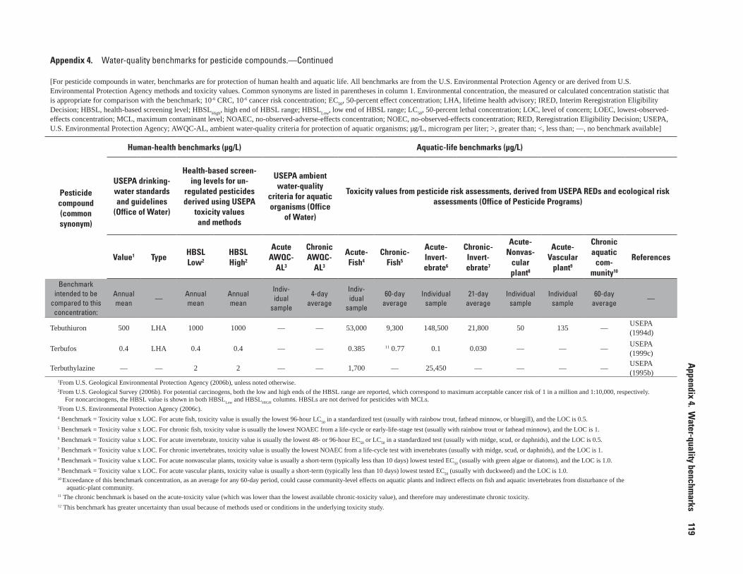
Appendix 4. Water-quality benchm
arks 119
Appendix 4. Water-quality benchmarks for pesticide compounds.—Continued [For pesticide compounds in water, benchmarks are for protection of human health and aquatic life. All benchmarks are from the U.S. Environmental Protection Agency or are derived from U.S. Environmental Protection Agency methods and toxicity values. Common synonyms are listed in parentheses in column 1. Environmental concentration, the measured or calculated concentration statistic that is appropriate for comparison with the benchmark; 10-6 CRC, 10-6 cancer risk concentration; EC
50, 50-percent effect concentration; LHA, lifetime health advisory; IRED, Interim Reregistration Eligibility
Decision; HBSL, health-based screening level; HBSLHigh
, high end of HBSL range; HBSLLow
, low end of HBSL range; LC50
, 50-percent lethal concentration; LOC, level of concern; LOEC, lowest-observed-effects concentration; MCL, maximum contaminant level; NOAEC, no-observed-adverse-effects concentration; NOEC, no-observed-effects concentration; RED, Reregistration Eligibility Decision; USEPA, U.S. Environmental Protection Agency; AWQC-AL, ambient water-quality criteria for protection of aquatic organisms; µg/L, microgram per liter; >, greater than; <, less than; —, no benchmark available]
Pesticide compound (common synonym)
Human-health benchmarks (µg/L) Aquatic-life benchmarks (µg/L)
USEPA drinking-water standards and guidelines
(Office of Water)
Health-based screen-ing levels for un-
regulated pesticides derived using USEPA
toxicity values and methods
USEPA ambient water-quality
criteria for aquatic organisms (Office
of Water)
Toxicity values from pesticide risk assessments, derived from USEPA REDs and ecological risk assessments (Office of Pesticide Programs)
Value1 TypeHBSLLow2
HBSLHigh2
Acute AWQC-
AL3
Chronic AWQC-
AL3
Acute-Fish4
Chronic-Fish5
Acute-Invert-ebrate6
Chronic-Invert-ebrate7
Acute-Nonvas-
cular plant8
Acute-Vascular
plant9
Chronic aquatic
com -munity10
References
Benchmark intended to be
compared to this concentration:
Annual mean
—Annual mean
Annual mean
Indiv-idual
sample
4-day average
Indiv-idual
sample
60-day average
Individual sample
21-day average
Individual sample
Individual sample
60-day average
—
Tebuthiuron 500 LHA 1000 1000 — — 53,000 9,300 148,500 21,800 50 135 —USEPA (1994d)
Terbufos 0.4 LHA 0.4 0.4 — — 0.385 11 0.77 0.1 0.030 — — —USEPA (1999c)
Terbuthylazine — — 2 2 — — 1,700 — 25,450 — — — —USEPA (1995b)
1From U.S. Geological Environmental Protection Agency (2006b), unless noted otherwise.2From U.S. Geological Survey (2006b). For potential carcinogens, both the low and high ends of the HBSL range are reported, which correspond to maximum acceptable cancer risk of 1 in a million and 1:10,000, respectively.
For noncarcinogens, the HBSL value is shown in both HBSLLow
and HBSLHIGH
columns. HBSLs are not derived for pesticides with MCLs.3From U.S. Environmental Protection Agency (2006c).4 Benchmark = Toxicity value x LOC. For acute fish, toxicity value is usually the lowest 96-hour LC
50 in a standardized test (usually with rainbow trout, fathead minnow, or bluegill), and the LOC is 0.5.
5 Benchmark = Toxicity value x LOC. For chronic fish, toxicity value is usually the lowest NOAEC from a life-cycle or early-life-stage test (usually with rainbow trout or fathead minnow), and the LOC is 1.6 Benchmark = Toxicity value x LOC. For acute invertebrate, toxicity value is usually the lowest 48- or 96-hour EC
50 or LC
50 in a standardized test (usually with midge, scud, or daphnids), and the LOC is 0.5.
7 Benchmark = Toxicity value x LOC. For chronic invertebrates, toxicity value is usually the lowest NOAEC from a life-cycle test with invertebrates (usually with midge, scud, or daphnids), and the LOC is 1.8 Benchmark = Toxicity value x LOC. For acute nonvascular plants, toxicity value is usually a short-term (typically less than 10 days) lowest tested EC
50 (usually with green algae or diatoms), and the LOC is 1.0.
9 Benchmark = Toxicity value x LOC. For acute vascular plants, toxicity value is usually a short-term (typically less than 10 days) lowest tested EC50
(usually with duckweed) and the LOC is 1.0.10 Exceedance of this benchmark concentration, as an average for any 60-day period, could cause community-level effects on aquatic plants and indirect effects on fish and aquatic invertebrates from disturbance of the
aquatic-plant community.11 The chronic benchmark is based on the acute-toxicity value (which was lower than the lowest available chronic-toxicity value), and therefore may underestimate chronic toxicity.12 This benchmark has greater uncertainty than usual because of methods used or conditions in the underlying toxicity study.
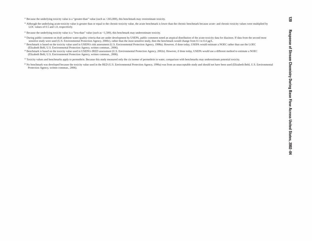
120
Response of Stream Chem
istry During Base Flow Across United States, 2002–04
13 Because the underlying toxicity value is a “greater-than” value (such as >265,000), this benchmark may overestimate toxicity.
14 Although the underlying acute-toxicity value is greater than or equal to the chronic-toxicity value, the acute benchmark is lower than the chronic benchmark because acute- and chronic-toxicity values were multiplied by LOC values of 0.5 and 1.0, respectively.
15 Because the underlying toxicity value is a “less-than” value (such as <1,500), this benchmark may underestimate toxicity.
16 During public comment on draft ambient water-quality criteria that are under development by USEPA, public comment noted an atypical distribution of the acute-toxicity data for diazinon. If data from the second most sensitive study were used (U.S. Environmental Protection Agency, 2000c), rather than the most sensitive study, then the benchmark would change from 0.1 to 0.4 µg/L.
17 Benchmark is based on the toxicity value used in USEPA’s risk assessment (U.S. Environmental Protection Agency, 1998a). However, if done today, USEPA would estimate a NOEC rather than use the LOEC (Elizabeth Behl, U.S. Environmental Protection Agency, written commun., 2006).
18 Benchmark is based on the toxicity value used in USEPA’s IRED assessment (U.S. Environmental Protection Agency, 2002e). However, if done today, USEPA would use a different method to estimate a NOEC (Elizabeth Behl, U.S. Environmental Protection Agency, written commun., 2006).
19 Toxicity values and benchmarks apply to permethrin. Because this study measured only the cis isomer of permethrin in water, comparison with benchmarks may underestimate potential toxicity.
20 No benchmark was developed because the toxicity value used in the RED (U.S. Environmental Protection Agency, 1996a) was from an unacceptable study and should not have been used (Elizabeth Behl, U.S. Environmental Protection Agency, written commun., 2006).
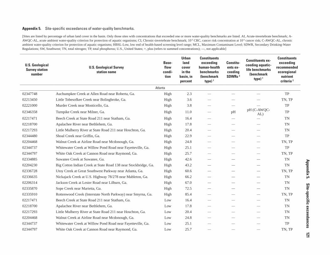
Appendix 5. Site-specific exceedances of water-quality benchmarks.
[Sites are listed by percentage of urban land cover in the basin. Only those sites with concentrations that exceeded one or more water-quality benchmarks are listed. AI, Acute-invertebrate benchmark; A-AWQC-AL, acute ambient water-quality criterion for protection of aquatic organisms; CI, Chronic-invertebrate benchmark; 10-6 CRC, cancer risk concentration at 10-6 cancer risk; C-AWQC-AL, chronic ambient water-quality criterion for protection of aquatic organisms; HBSL-Low, low end of health-based screening level range; MCL, Maximum Contaminant Level; SDWR, Secondary Drinking-Water Regulations; SW, Southwest; TN, total nitrogen; TP, total phosphorus; U.S., United States; +, plus (refers to summed concentrations); —, not applicable]
U.S. Geological Survey station
number
U.S. Geological Survey station name
Base-flow
condi-tion
Urban land
cover in the
basin, in percent
Constituents exceeding
human-health benchmarks (benchmark
type) 1
Constitu-ents ex-ceeding SDWRs 2
Constituents ex-ceeding aquatic-life benchmarks
(benchmark type) 1
Constituents exceeding
recommended ecoregional
nutrient criteria 2
Atlanta
02347748 Auchumpkee Creek at Allen Road near Roberta, Ga. High 2.3 — — — TP
02213450 Little Tobesofkee Creek near Bolingbroke, Ga. High 3.6 — — — TN, TP
02221000 Murder Creek near Monticello, Ga. High 3.8 — — — TP
02346358 Turnpike Creek near Milner, Ga. High 11.0 — pH pH (C-AWQC-AL) TP
02217471 Beech Creek at State Road 211 near Statham, Ga. High 16.4 — — — TN
02218700 Apalachee River near Bethlehem, Ga. High 17.8 — — — TN
02217293 Little Mulberry River at State Road 211 near Hoschton, Ga. High 20.4 — — — TN
02344480 Shoal Creek near Griffin, Ga. High 22.9 — — — TP
02204468 Walnut Creek at Airline Road near Mcdonough, Ga. High 24.8 — — — TN, TP
02344737 Whitewater Creek at Willow Pond Road near Fayetteville, Ga. High 25.1 — — — TP
02344797 White Oak Creek at Cannon Road near Raymond, Ga. High 25.7 — — — TN, TP
02334885 Suwanee Creek at Suwanee, Ga. High 42.6 — — — TN
02204230 Big Cotton Indian Creek at State Road 138 near Stockbridge, Ga. High 43.2 — — — TN
02336728 Utoy Creek at Great Southwest Parkway near Atlanta, Ga. High 60.6 — — — TN, TP
02336635 Nickajack Creek at U.S. Highway 78/278 near Mableton, Ga. High 66.2 — — — TN
02206314 Jackson Creek at Lester Road near Lilburn, Ga. High 67.0 — — — TN
02335870 Sope Creek near Marietta, Ga. High 72.5 — — — TN
02335910 Rottenwood Creek (Interstate North Parkway) near Smyrna, Ga. High 85.4 — — — TN, TP
02217471 Beech Creek at State Road 211 near Statham, Ga. Low 16.4 — — — TN
02218700 Apalachee River near Bethlehem, Ga. Low 17.8 — — — TN
02217293 Little Mulberry River at State Road 211 near Hoschton, Ga. Low 20.4 — — — TN
02204468 Walnut Creek at Airline Road near Mcdonough, Ga. Low 24.8 — — — TN
02344737 Whitewater Creek at Willow Pond Road near Fayetteville, Ga. Low 25.1 — — — TP
02344797 White Oak Creek at Cannon Road near Raymond, Ga. Low 25.7 — — — TN, TP
Appendix 5. Site-specific exceedances
121
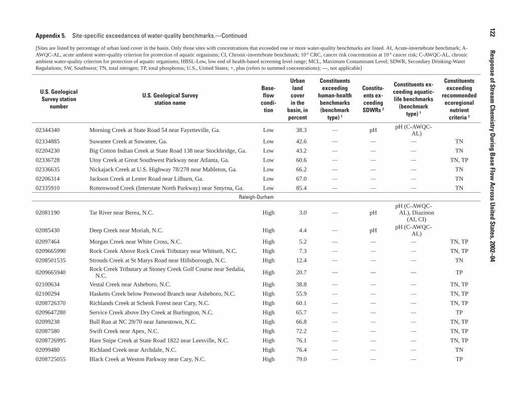
Appendix 5. Site-specific exceedances of water-quality benchmarks.—Continued
[Sites are listed by percentage of urban land cover in the basin. Only those sites with concentrations that exceeded one or more water-quality benchmarks are listed. AI, Acute-invertebrate benchmark; A-AWQC-AL, acute ambient water-quality criterion for protection of aquatic organisms; CI, Chronic-invertebrate benchmark; 10-6 CRC, cancer risk concentration at 10-6 cancer risk; C-AWQC-AL, chronic ambient water-quality criterion for protection of aquatic organisms; HBSL-Low, low end of health-based screening level range; MCL, Maximum Contaminant Level; SDWR, Secondary Drinking-Water Regulations; SW, Southwest; TN, total nitrogen; TP, total phosphorus; U.S., United States; +, plus (refers to summed concentrations); —, not applicable]
U.S. Geological Survey station
number
U.S. Geological Survey station name
Base-flow
condi-tion
Urban land
cover in the
basin, in percent
Constituents exceeding
human-health benchmarks (benchmark
type) 1
Constitu-ents ex-ceeding SDWRs 2
Constituents ex-ceeding aquatic-life benchmarks
(benchmark type) 1
Constituents exceeding
recommended ecoregional
nutrient criteria 2
02344340 Morning Creek at State Road 54 near Fayetteville, Ga. Low 38.3 — pH pH (C-AWQC-AL)
02334885 Suwanee Creek at Suwanee, Ga. Low 42.6 — — — TN
02204230 Big Cotton Indian Creek at State Road 138 near Stockbridge, Ga. Low 43.2 — — — TN
02336728 Utoy Creek at Great Southwest Parkway near Atlanta, Ga. Low 60.6 — — — TN, TP
02336635 Nickajack Creek at U.S. Highway 78/278 near Mableton, Ga. Low 66.2 — — — TN
02206314 Jackson Creek at Lester Road near Lilburn, Ga. Low 67.0 — — — TN
02335910 Rottenwood Creek (Interstate North Parkway) near Smyrna, Ga. Low 85.4 — — — TN
Raleigh-Durham
02081190 Tar River near Berea, N.C. High 3.0 — pHpH (C-AWQC-
AL), Diazinon (AI, CI)
02085430 Deep Creek near Moriah, N.C. High 4.4 — pH pH (C-AWQC-AL)
02097464 Morgan Creek near White Cross, N.C. High 5.2 — — — TN, TP
0209665990 Rock Creek Above Rock Creek Tributary near Whitsett, N.C. High 7.3 — — — TN, TP
0208501535 Strouds Creek at St Marys Road near Hillsborough, N.C. High 12.4 — — — TN
0209665940 Rock Creek Tributary at Stoney Creek Golf Course near Sedalia, N.C. High 20.7 — — — TP
02100634 Vestal Creek near Asheboro, N.C. High 38.8 — — — TN, TP
02100294 Hasketts Creek below Penwood Branch near Asheboro, N.C. High 55.9 — — — TN, TP
0208726370 Richlands Creek at Schenk Forest near Cary, N.C. High 60.1 — — — TN, TP
0209647280 Service Creek above Dry Creek at Burlington, N.C. High 65.7 — — — TP
02099238 Bull Run at NC 29/70 near Jamestown, N.C. High 66.8 — — — TN, TP
02087580 Swift Creek near Apex, N.C. High 72.2 — — — TN, TP
0208726995 Hare Snipe Creek at State Road 1822 near Leesville, N.C. High 76.1 — — — TN, TP
02099480 Richland Creek near Archdale, N.C. High 76.4 — — — TN
0208725055 Black Creek at Weston Parkway near Cary, N.C. High 79.0 — — — TP
122
Response of Stream Chem
istry During Base Flow Across United States, 2002–04

Appendix 5. Site-specific exceedances
123Appendix 5. Site-specific exceedances of water-quality benchmarks.—Continued
[Sites are listed by percentage of urban land cover in the basin. Only those sites with concentrations that exceeded one or more water-quality benchmarks are listed. AI, Acute-invertebrate benchmark; A-AWQC-AL, acute ambient water-quality criterion for protection of aquatic organisms; CI, Chronic-invertebrate benchmark; 10-6 CRC, cancer risk concentration at 10-6 cancer risk; C-AWQC-AL, chronic ambient water-quality criterion for protection of aquatic organisms; HBSL-Low, low end of health-based screening level range; MCL, Maximum Contaminant Level; SDWR, Secondary Drinking-Water Regulations; SW, Southwest; TN, total nitrogen; TP, total phosphorus; U.S., United States; +, plus (refers to summed concentrations); —, not applicable]
U.S. Geological Survey station
number
U.S. Geological Survey station name
Base-flow
condi-tion
Urban land
cover in the
basin, in percent
Constituents exceeding
human-health benchmarks (benchmark
type) 1
Constitu-ents ex-ceeding SDWRs 2
Constituents ex-ceeding aquatic-life benchmarks
(benchmark type) 1
Constituents exceeding
recommended ecoregional
nutrient criteria 2
0209679804 Little Alamance Creek at State Road 2309 near Graham, N.C. High 82.1 — — — TN, TP
0209651815 Branch Creek below NC54 near Graham, N.C. High 92.6 — — — TN
02087304 SW Prong Beaverdam Creek at Raleigh, N.C. High 94.2Dieldrin (10-6 CRC,
HBSL-Low)— — TN
0209647295 Dry Creek above Service Creek at Burlington, N.C. High 96.8 — — — TN, TP
0211583580 Bowen Branch near Mouth at Winston-Salem, N.C. High 96.9 — —Ammonia (C-
AWQC-AL) TN
0209517912 North Buffalo Creek at Greensboro, N.C. High 96.9 — — — TN, TP
0208732610 Pigeon House Br at Crabtree Boulevard at Raleigh, N.C. High 98.4Dieldrin (10-6 CRC,
HBSL-Low)— — TN
0209695780 Brooks Creek at Eddie Perry Road near Bynum, N.C. Low 3.1 — — — TN
02097464 Morgan Creek near White Cross, N.C. Low 5.2 — — — TN, TP
0209697900 Pokeberry Creek near Pittsboro, N.C. Low 6.0 — — — TP
0209665990 Rock Creek above Rock Creek Tributary near Whitsett, N.C. Low 7.3 — — — TN, TP
0208794025 Camp Branch above State Road 1390 near Holly Springs, N.C. Low 18.2 — — — TP
0208500600 Strouds Creek at St Marys Road near Hillsborough, N.C. Low 20.0 — — — TN
0209665940 Rock Creek Tributary at Stoney Creek Golf Course near Sedalia, N.C. Low 20.7 — — — TP
02100634 Vestal Creek near Asheboro, N.C. Low 38.8 — — — TP
0208758440 Dutchmans Branch at State Road 1386 near McCullers Crossroads, N.C. Low 39.3 — — — TP
02097355 Bolin Creek above Franklin Street near Chapel Hill, N.C. Low 44.3 — —Diazinon (AI,
CI) TN, TP
02081510 Foundry Branch at Mouth near Oxford, N.C. Low 53.0 — — — TN, TP
02100294 Hasketts Creek Below Penwood Branch near Asheboro, N.C. Low 55.9 — — — TP
0209647280 Service Creek above Dry Creek at Burlington, N.C. Low 65.7 — pH pH (C-AWQC-AL) TN, TP
02099238 Bull Run at NC 29/70 near Jamestown, N.C. Low 66.8 — — — TN, TP

124
Response of Stream Chem
istry During Base Flow Across United States, 2002–04
Appendix 5. Site-specific exceedances of water-quality benchmarks.—Continued
[Sites are listed by percentage of urban land cover in the basin. Only those sites with concentrations that exceeded one or more water-quality benchmarks are listed. AI, Acute-invertebrate benchmark; A-AWQC-AL, acute ambient water-quality criterion for protection of aquatic organisms; CI, Chronic-invertebrate benchmark; 10-6 CRC, cancer risk concentration at 10-6 cancer risk; C-AWQC-AL, chronic ambient water-quality criterion for protection of aquatic organisms; HBSL-Low, low end of health-based screening level range; MCL, Maximum Contaminant Level; SDWR, Secondary Drinking-Water Regulations; SW, Southwest; TN, total nitrogen; TP, total phosphorus; U.S., United States; +, plus (refers to summed concentrations); —, not applicable]
U.S. Geological Survey station
number
U.S. Geological Survey station name
Base-flow
condi-tion
Urban land
cover in the
basin, in percent
Constituents exceeding
human-health benchmarks (benchmark
type) 1
Constitu-ents ex-ceeding SDWRs 2
Constituents ex-ceeding aquatic-life benchmarks
(benchmark type) 1
Constituents exceeding
recommended ecoregional
nutrient criteria 2
02087580 Swift Creek near Apex, N.C. Low 72.2 — — — TP
0208726995 Hare Snipe Creek at State Road 1822 near Leesville, N.C. Low 76.1 — — — TN
02099480 Richland Creek near Archdale, N.C. Low 76.4 — — — TN
0208725055 Black Creek at Weston Parkway near Cary, N.C. Low 79.0 — — — TN, TP
0209679804 Little Alamance Creek at State Road 2309 near Graham, N.C. Low 82.1 — — — TN, TP
0209651815 Branch Creek Below NC54 near Graham, N.C. Low 92.6 — — — TN, TP
02087304 SW Prong Beaverdam Creek at Raleigh, N.C. Low 94.2Dieldrin (10-6 CRC,
HBSL-Low)— — TN
0209647295 Dry Creek above Service Creek at Burlington, N.C. Low 96.8 — — — TN, TP
0211583580 Bowen Branch near Mouth at Winston-Salem, N.C. Low 96.9Dieldrin (10-6 CRC,
HBSL-Low)—
Ammonia (C-AWQC-AL) TN
0209517912 North Buffalo Creek at Greensboro, N.C. Low 96.9Dieldrin (10-6 CRC,
HBSL-Low)— — TN, TP
0208732610 Pigeon House Branch at Crabtree Boulevard at Raleigh, N.C. Low 98.4Dieldrin (10-6 CRC,
HBSL-Low)— — TN
Milwaukee-Green Bay
040853145 Black Creek at Curran Road near Denmark, Wis. High 3.2 — — — TN, TP
04085188 Rio Creek at Pheasant Road near Rio Creek, Wis. High 3.5 — — — TP
04085270 Jambo Creek at Jambo Creek Road near Mishicot, Wis. High 3.7 — — — TP
04085322 Devils River at Rosencrans Road near Maribel, Wis. High 4.0 — — — TP
040851932 Kewaunee River Tributary at Lowell Road near Luxemburg, Wis. High 4.4 — — — TN, TP
040854395 Point Creek at Ucker Point Road near Newton, Wis. High 5.0 — — — TN, TP
04085455 Meeme River at Washington Road near Cleveland, Wis. High 5.0 — — — TN, TP

Appendix 5. Site-specific exceedances
125Appendix 5. Site-specific exceedances of water-quality benchmarks.—Continued
[Sites are listed by percentage of urban land cover in the basin. Only those sites with concentrations that exceeded one or more water-quality benchmarks are listed. AI, Acute-invertebrate benchmark; A-AWQC-AL, acute ambient water-quality criterion for protection of aquatic organisms; CI, Chronic-invertebrate benchmark; 10-6 CRC, cancer risk concentration at 10-6 cancer risk; C-AWQC-AL, chronic ambient water-quality criterion for protection of aquatic organisms; HBSL-Low, low end of health-based screening level range; MCL, Maximum Contaminant Level; SDWR, Secondary Drinking-Water Regulations; SW, Southwest; TN, total nitrogen; TP, total phosphorus; U.S., United States; +, plus (refers to summed concentrations); —, not applicable]
U.S. Geological Survey station
number
U.S. Geological Survey station name
Base-flow
condi-tion
Urban land
cover in the
basin, in percent
Constituents exceeding
human-health benchmarks (benchmark
type) 1
Constitu-ents ex-ceeding SDWRs 2
Constituents ex-ceeding aquatic-life benchmarks
(benchmark type) 1
Constituents exceeding
recommended ecoregional
nutrient criteria 2
04078085 Black Otter Creek near Hortonville, Wis. High 5.4 — — — TN, TP
040851325 Baird Creek at Superior Road at Green Bay, Wis. High 5.5 — — — TP
04085068 Ashwaubenon Creek near Little Rapids, Wis. High 5.7 Atrazine (MCL)
— — TN, TP
05527729 Kilbourn Ditch at 6oth Street near Kenosha, Wis. High 7.4Nitrite+nitrate,
nitrate, atra-zine (MCL)
— — TN, TP
04072233 Lancaster Brook at Shawano Avenue at Howard, Wis. High 11.7 — — — TN, TP
04081897 Sawyer Creek at Westhaven Road at Oshkosh, Wis. High 13.8 — — — TN, TP
04086699 Pigeon Creek at Williamsburg Drive at Theinsville, Wis. High 14.9 — — — TN, TP
040872393 Hoods Creek at Brook Road near Franksville, Wis. High 16.3 — — — TN, TP
04085046 Apple Creek at Sniderville, Wis. High 17.6 — pH — TP
055437901 Fox River at River Road near Sussex, Wis. High 20.2 — — — TN, TP
040851235 Bower Creek Tributary at Lime Kiln Road near Bellevue, Wis. High 24.4 — — — TP
04087258 Pike River at County Highway A near Kenosha, Wis. High 27.3Nitrite+nitrate,
nitrate (MCL)
— — TN, TP
04087030 Menomonee River at Menomonee Falls, Wis. High 30.4 — — — TN, TP
04084429 Mud Creek at Spencer Road at Appleton, Wis. High 58.8 — — — TN, TP
04087204 Oak Creek at South Milwaukee, Wis. High 62.9 — — — TN, TP
04084468 Garners Creek at Park Street at Kaukauna, Wis. High 68.9 — — — TN, TP
0408703164 Lily Creek at Good Hope Road near Menomonee Falls, Wis. High 78.0 — — — TN, TP
040870856 Underwood Creek at Watertown Plank Road at Elm Grove, Wis. High 86.0 — — — TN, TP
04087270 Pike Creek at 43rd Street at Kenosha, Wis. High 87.2 — — — TN
04087213 Root River at Layton Avenue at Greenfield, Wis. High 92.8 — — — TN, TP
040869415 Lincoln Creek at 47th Street at Milwaukee, Wis. High 97.6 — — — TN, TP
04087118 Honey Creek near Portland Avenue at Wauwatosa, Wis. High 99.1 — — — TN, TP

126
Response of Stream Chem
istry During Base Flow Across United States, 2002–04
Appendix 5. Site-specific exceedances of water-quality benchmarks.—Continued
[Sites are listed by percentage of urban land cover in the basin. Only those sites with concentrations that exceeded one or more water-quality benchmarks are listed. AI, Acute-invertebrate benchmark; A-AWQC-AL, acute ambient water-quality criterion for protection of aquatic organisms; CI, Chronic-invertebrate benchmark; 10-6 CRC, cancer risk concentration at 10-6 cancer risk; C-AWQC-AL, chronic ambient water-quality criterion for protection of aquatic organisms; HBSL-Low, low end of health-based screening level range; MCL, Maximum Contaminant Level; SDWR, Secondary Drinking-Water Regulations; SW, Southwest; TN, total nitrogen; TP, total phosphorus; U.S., United States; +, plus (refers to summed concentrations); —, not applicable]
U.S. Geological Survey station
number
U.S. Geological Survey station name
Base-flow
condi-tion
Urban land
cover in the
basin, in percent
Constituents exceeding
human-health benchmarks (benchmark
type) 1
Constitu-ents ex-ceeding SDWRs 2
Constituents ex-ceeding aquatic-life benchmarks
(benchmark type) 1
Constituents exceeding
recommended ecoregional
nutrient criteria 2
040853145 Black Creek at Curran Road near Denmark, Wis. Low 3.2 — —
Chlorpyrifos (A-AWQC-AL,
C-AWQC-AL, AI, CI), Mala-thion (CI, C-AWQC-AL)
TN, TP
04085188 Rio Creek at Pheasant Road near Rio Creek, Wis. Low 3.5 — — — TN, TP
04085270 Jambo Creek at Jambo Creek Road near Mishicot, Wis. Low 3.7 — — — TN
04085322 Devils River at Rosencrans Road near Maribel, Wis. Low 4.0 — — — TN, TP
040851932 Kewaunee River Tributary at Lowell Road near Luxemburg, Wis. Low 4.4 — — — TP
040854395 Point Creek at Ucker Point Road near Newton, Wis. Low 5.0 — — — TP
04085455 Meeme River at Washington Road near Cleveland, Wis. Low 5.0 — — — TN, TP
04078085 Black Otter Creek near Hortonville, Wis. Low 5.4 — — — TN, TP
040851325 Baird Creek at Superior Road at Green Bay, Wis. Low 5.5 — — — TP
040850683 Ashwaubenon Creek at South Bridge Road near Depere, Wis. Low 5.7 — — — TN, TP
05527729 Kilbourn Ditch at 6oth Street near Kenosha, Wis. Low 7.4 — — — TP
04072233 Lancaster Brook at Shawano Avenue at Howard, Wis. Low 11.7 — — — TN, TP
04081897 Sawyer Creek at Westhaven Road at Oshkosh, Wis. Low 13.8 — — — TP
04086699 Pigeon Creek at Williamsburg Drive at Theinsville, Wis. Low 14.9 — — — TP
040872393 Hoods Creek at Brook Road near Franksville, Wis. Low 16.3 — — — TN, TP
04085046 Apple Creek at Sniderville, Wis. Low 17.6 — — — TN, TP
055437901 Fox River at River Road near Sussex, Wis. Low 20.2 — — — TN, TP
040851235 Bower Creek Tributary at Lime Kiln Road near Bellevue, Wis. Low 24.4 — — — TP
04087258 Pike River at County Highway A near Kenosha, Wis. Low 27.3 — — — TN, TP
04087030 Menomonee River at Menomonee Falls, Wis. Low 30.4 — — — TP
04087070 Little Menomonee River at Milwaukee, Wis. Low 44.3 — — — TP
04084429 Mud Creek at Spencer Road at Appleton, Wis. Low 58.8 — — — TP

Appendix 5. Site-specific exceedances
127Appendix 5. Site-specific exceedances of water-quality benchmarks.—Continued
[Sites are listed by percentage of urban land cover in the basin. Only those sites with concentrations that exceeded one or more water-quality benchmarks are listed. AI, Acute-invertebrate benchmark; A-AWQC-AL, acute ambient water-quality criterion for protection of aquatic organisms; CI, Chronic-invertebrate benchmark; 10-6 CRC, cancer risk concentration at 10-6 cancer risk; C-AWQC-AL, chronic ambient water-quality criterion for protection of aquatic organisms; HBSL-Low, low end of health-based screening level range; MCL, Maximum Contaminant Level; SDWR, Secondary Drinking-Water Regulations; SW, Southwest; TN, total nitrogen; TP, total phosphorus; U.S., United States; +, plus (refers to summed concentrations); —, not applicable]
U.S. Geological Survey station
number
U.S. Geological Survey station name
Base-flow
condi-tion
Urban land
cover in the
basin, in percent
Constituents exceeding
human-health benchmarks (benchmark
type) 1
Constitu-ents ex-ceeding SDWRs 2
Constituents ex-ceeding aquatic-life benchmarks
(benchmark type) 1
Constituents exceeding
recommended ecoregional
nutrient criteria 2
04087204 Oak Creek at South Milwaukee, Wis. Low 62.9 — — — TN, TP
04084468 Garners Creek at Park Street at Kaukauna, Wis. Low 68.9 — — — TP
0408703164 Lily Creek at Good Hope Road near Menomonee Falls, Wis. Low 78.0 — — — TP
040870856 Underwood Creek at Watertown Plank Road at Elm Grove, Wis. Low 86.0 — — — TP
04087270 Pike Creek at 43rd Street at Kenosha, Wis. Low 87.2 — — — TN
04087213 Root River at Layton Avenue at Greenfield, Wis. Low 92.8 — — — TN, TP
040869415 Lincoln Creek at 47th Street at Milwaukee, Wis. Low 97.6 — — — TP
04087118 Honey Creek near Portland Avenue at Wauwatosa, Wis. Low 99.1 — — — TN, TP
Dallas-Fort Worth
08062805 Williams Creek near Farm to Market 1836 near Kemp, Tex. High 1.6 — — — TP
08063595 South Prong Creek at Farm to Market 876 near Waxahachie, Tex. High 2.3 — — — TN
08062600 Grays Creek at Creek 1603 near Rice, Tex. High 2.5 — Chloride Chloride (C-AWQC-AL) TP
08063047 Bynum Creek near Farm to Market 308 near Malone, Tex. High 2.7 — — — TN
08063565 Mill Creek at Lowell Road near Milford, Tex. High 2.8 — — — TN
08063300 Pin Oak Creek near Farm to Market 73 near Coolidge, Tex. High 3.1 — — — TP
08063555 South Fork Chambers Creek near Creek 102 near Maypearl, Tex. High 3.3 — Sulfate —
08049580 Mountain Creek near Venus, Tex. High 4.8 — Sulfate —
08059571 Wilson Creek near Gray Branch Road near Mckinney, Tex. High 6.5 — — — TN
08052740 Doe Branch at Fishtrap Road near Prosper, Tex. High 6.7 Atrazine (MCL)
— — TN, TP
08064695 Tehuacana Creek at Rural Road 27 near Wortham, Tex. High 6.9 — pH —
08062020 Buffalo Creek near Farm to Market 148 near Crandall, Tex. High 7.2 — — — TN, TP
08061780 Buffalo Creek near Trinity Road at Forney, Tex. High 15.2 — — — TN, TP
08061995 Mustang Creek at Farm to Market 2757 near Crandall, Tex. High 17.3 — — — TN, TP
08057475 Parsons Slough near Davis Road near Crandall, Tex. High 21.3 — — — TP
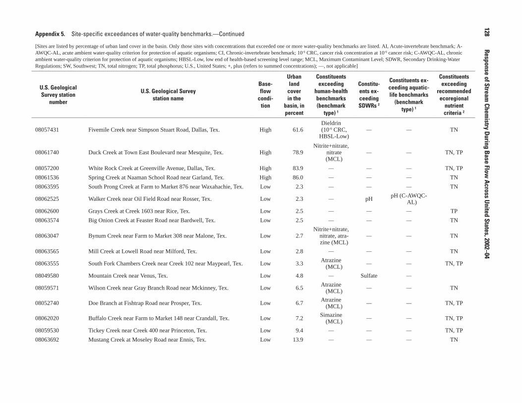
128
Response of Stream Chem
istry During Base Flow Across United States, 2002–04
Appendix 5. Site-specific exceedances of water-quality benchmarks.—Continued
[Sites are listed by percentage of urban land cover in the basin. Only those sites with concentrations that exceeded one or more water-quality benchmarks are listed. AI, Acute-invertebrate benchmark; A-AWQC-AL, acute ambient water-quality criterion for protection of aquatic organisms; CI, Chronic-invertebrate benchmark; 10-6 CRC, cancer risk concentration at 10-6 cancer risk; C-AWQC-AL, chronic ambient water-quality criterion for protection of aquatic organisms; HBSL-Low, low end of health-based screening level range; MCL, Maximum Contaminant Level; SDWR, Secondary Drinking-Water Regulations; SW, Southwest; TN, total nitrogen; TP, total phosphorus; U.S., United States; +, plus (refers to summed concentrations); —, not applicable]
U.S. Geological Survey station
number
U.S. Geological Survey station name
Base-flow
condi-tion
Urban land
cover in the
basin, in percent
Constituents exceeding
human-health benchmarks (benchmark
type) 1
Constitu-ents ex-ceeding SDWRs 2
Constituents ex-ceeding aquatic-life benchmarks
(benchmark type) 1
Constituents exceeding
recommended ecoregional
nutrient criteria 2
08057431 Fivemile Creek near Simpson Stuart Road, Dallas, Tex. High 61.6Dieldrin (10-6 CRC,
HBSL-Low)— — TN
08061740 Duck Creek at Town East Boulevard near Mesquite, Tex. High 78.9Nitrite+nitrate,
nitrate (MCL)
— — TN, TP
08057200 White Rock Creek at Greenville Avenue, Dallas, Tex. High 83.9 — — — TN, TP
08061536 Spring Creek at Naaman School Road near Garland, Tex. High 86.0 — — — TN
08063595 South Prong Creek at Farm to Market 876 near Waxahachie, Tex. Low 2.3 — — — TN
08062525 Walker Creek near Oil Field Road near Rosser, Tex. Low 2.3 — pH pH (C-AWQC-AL)
08062600 Grays Creek at Creek 1603 near Rice, Tex. Low 2.5 — — — TP
08063574 Big Onion Creek at Feaster Road near Bardwell, Tex. Low 2.5 — — — TN
08063047 Bynum Creek near Farm to Market 308 near Malone, Tex. Low 2.7Nitrite+nitrate,
nitrate, atra-zine (MCL)
— — TN
08063565 Mill Creek at Lowell Road near Milford, Tex. Low 2.8 — — — TN
08063555 South Fork Chambers Creek near Creek 102 near Maypearl, Tex. Low 3.3 Atrazine (MCL)
— — TN, TP
08049580 Mountain Creek near Venus, Tex. Low 4.8 — Sulfate —
08059571 Wilson Creek near Gray Branch Road near Mckinney, Tex. Low 6.5 Atrazine (MCL)
— — TN
08052740 Doe Branch at Fishtrap Road near Prosper, Tex. Low 6.7 Atrazine (MCL)
— — TN, TP
08062020 Buffalo Creek near Farm to Market 148 near Crandall, Tex. Low 7.2 Simazine (MCL)
— — TN, TP
08059530 Tickey Creek near Creek 400 near Princeton, Tex. Low 9.4 — — — TN, TP
08063692 Mustang Creek at Moseley Road near Ennis, Tex. Low 13.9 — — — TN

Appendix 5. Site-specific exceedances
129Appendix 5. Site-specific exceedances of water-quality benchmarks.—Continued
[Sites are listed by percentage of urban land cover in the basin. Only those sites with concentrations that exceeded one or more water-quality benchmarks are listed. AI, Acute-invertebrate benchmark; A-AWQC-AL, acute ambient water-quality criterion for protection of aquatic organisms; CI, Chronic-invertebrate benchmark; 10-6 CRC, cancer risk concentration at 10-6 cancer risk; C-AWQC-AL, chronic ambient water-quality criterion for protection of aquatic organisms; HBSL-Low, low end of health-based screening level range; MCL, Maximum Contaminant Level; SDWR, Secondary Drinking-Water Regulations; SW, Southwest; TN, total nitrogen; TP, total phosphorus; U.S., United States; +, plus (refers to summed concentrations); —, not applicable]
U.S. Geological Survey station
number
U.S. Geological Survey station name
Base-flow
condi-tion
Urban land
cover in the
basin, in percent
Constituents exceeding
human-health benchmarks (benchmark
type) 1
Constitu-ents ex-ceeding SDWRs 2
Constituents ex-ceeding aquatic-life benchmarks
(benchmark type) 1
Constituents exceeding
recommended ecoregional
nutrient criteria 2
08061780 Buffalo Creek near Trinity Road at Forney, Tex. Low 15.2 — — — TN, TP
08061995 Mustang Creek at Farm to Market 2757 near Crandall, Tex. Low 17.3 — pH — TP
08057475 Parsons Slough near Davis Road near Crandall, Tex. Low 21.3 — — — TP
08061952 South Mesquite Creek at Lawson Road near Mesquite, Tex. Low 71.9 — — — TP
08061740 Duck Creek at Town East Boulevard near Mesquite, Tex. Low 78.9Nitrite+nitrate,
nitrate (MCL)
— — TN, TP
08057200 White Rock Creek at Greenville Avenue, Dallas, Tex. Low 83.9 — — — TN, TP
08061536 Spring Creek at Naaman School Road near Garland, Tex. Low 86.0 Atrazine (MCL)
— — TN
08049490 Johnson Creek near Duncan Perry Road, Grand Prairie, Tex. Low 88.8 — pH pH (C-AWQC-AL)
Denver
403308105001601 Boxelder Creek at Mouth near Fort Collins, Colo. High 4.4 — Sulfate — TN
400855105090501 Dry Creek below Airport Road near Longmont, Colo. High 8.7 — Sulfate — TN, TP
410714104480101 Crow Creek above Morrie Avenue at Cheyenne, Wyo. High 8.7 — — — TN, TP
400810105071301 Left Hand Creek above Pike Road at Longmont, Colo. High 10.4 — — — TN
403048105042701 Fossil Creek at College Avenue at Fort Collins, Colo. High 16.6 — Sulfate — TN
395554105085601 Rock Creek above Rock Creek Parkway at Superior, Colo. High 17.4 — — — TN
400607105094401 Dry Creek below Niwot Road at Niwot, Colo. High 22.2 — Sulfate — TN, TP
400925105023201 Spring Gulch at Sandstone Ranch Park near Longmont, Colo. High 25.2 — Sulfate — TN, TP
395324105035001 Big Dry Creek below Hyland Circle at Westminster, Colo. High 33.3 — pH —
394919105074601 Ralston Creek above Simms at Arvada, Colo. High 41.4 — — — TP
393613104511401 Cottonwood Creek above Newark Way at Greenwood Village, Colo. High 59.1 — Sulfate — TN, TP
394629105063101 Clear Creek below Kipling at Wheat Ridge, Colo. High 62.6 — — — TP
403356105024001 Spring Creek at Edora Park at Fort Collins, Colo. High 63.5 — — — TN, TP
394553105075101 Lena Gulch at Lewis Meadows Park at Wheat Ridge, Colo. High 68.8 — — — TP

130
Response of Stream Chem
istry During Base Flow Across United States, 2002–04
Appendix 5. Site-specific exceedances of water-quality benchmarks.—Continued
[Sites are listed by percentage of urban land cover in the basin. Only those sites with concentrations that exceeded one or more water-quality benchmarks are listed. AI, Acute-invertebrate benchmark; A-AWQC-AL, acute ambient water-quality criterion for protection of aquatic organisms; CI, Chronic-invertebrate benchmark; 10-6 CRC, cancer risk concentration at 10-6 cancer risk; C-AWQC-AL, chronic ambient water-quality criterion for protection of aquatic organisms; HBSL-Low, low end of health-based screening level range; MCL, Maximum Contaminant Level; SDWR, Secondary Drinking-Water Regulations; SW, Southwest; TN, total nitrogen; TP, total phosphorus; U.S., United States; +, plus (refers to summed concentrations); —, not applicable]
U.S. Geological Survey station
number
U.S. Geological Survey station name
Base-flow
condi-tion
Urban land
cover in the
basin, in percent
Constituents exceeding
human-health benchmarks (benchmark
type) 1
Constitu-ents ex-ceeding SDWRs 2
Constituents ex-ceeding aquatic-life benchmarks
(benchmark type) 1
Constituents exceeding
recommended ecoregional
nutrient criteria 2
393557105033101 Dutch Creek at Weaver Park near Columbine Valley, Colo. High 72.0 — Sulfate — TN
06713500 Cherry Creek at Denver, Colo. High 79.6 — — — TN, TP
394409105020501 Lakewood Gulch above Knox Street at Denver, Colo. High 89.3 — — — TN
394107105021001 Sanderson Gulch above Lowell Avenue at Denver, Colo. High 90.4 — pH — TN
403308105001601 Boxelder Creek at Mouth near Fort Collins, Colo. Low 4.4 — Sulfate — TN
400855105090501 Dry Creek below Airport Road near Longmont, Colo. Low 8.7 — Sulfate — TN, TP
410714104480101 Crow Creek above Morrie Avenue at Cheyenne, Wyo. Low 8.7 — —Malathion (CI,
C-AWQC-AL)
TN, TP
400810105071301 Left Hand Creek above Pike Road at Longmont, Colo. Low 10.4 — Sulfate — TN
403048105042701 Fossil Creek at College Avenue at Fort Collins, Colo. Low 16.6 — — — TN
395554105085601 Rock Creek above Rock Creek Parkway at Superior, Colo. Low 17.4 — — — TN, TP
402549105043101 Dry Creek at U.S. Highway 287 at Loveland, Colo. Low 20.9 — Sulfate — TN
400607105094401 Dry Creek below Niwot Road at Niwot, Colo. Low 22.2 — — — TN, TP
400925105023201 Spring Gulch at Sandstone Ranch Park near Longmont, Colo. Low 25.2 — Sulfate — TN
393948105053501 Bear Creek below Estes Road at Lakewood, Colo. Low 38.0 — — — TN, TP
394919105074601 Ralston Creek above Simms at Arvada, Colo. Low 41.4 — — — TN, TP
393613104511401 Cottonwood Creek above Newark Way at Greenwood Village, Colo. Low 59.1 — Sulfate — TN, TP
394629105063101 Clear Creek below Kipling at Wheat Ridge, Colo. Low 62.6 — — — TN, TP
403356105024001 Spring Creek at Edora Park at Fort Collins, Colo. Low 63.5 — — — TN, TP
393557105033101 Dutch Creek at Weaver Park near Columbine Valley, Colo. Low 72.0 — Sulfate — TN
06713500 Cherry Creek at Denver, Colo. Low 79.6 — — — TN, TP
403035105035301 Mail Creek near Mouth at Fort Collins, Colo. Low 88.1 — Sulfate — TN
394409105020501 Lakewood Gulch above Knox Street at Denver, Colo. Low 89.3 — — — TN
394107105021001 Sanderson Gulch above Lowell Ave at Denver, Colo. Low 90.4 — — — TN, TP
Portland
14205400 East Fork Dairy Creek near Meacham Corner, Oreg. High 0.5 — — — TN

Appendix 5. Site-specific exceedances of water-quality benchmarks.—Continued
[Sites are listed by percentage of urban land cover in the basin. Only those sites with concentrations that exceeded one or more water-quality benchmarks are listed. AI, Acute-invertebrate benchmark; A-AWQC-AL, acute ambient water-quality criterion for protection of aquatic organisms; CI, Chronic-invertebrate benchmark; 10-6 CRC, cancer risk concentration at 10-6 cancer risk; C-AWQC-AL, chronic ambient water-quality criterion for protection of aquatic organisms; HBSL-Low, low end of health-based screening level range; MCL, Maximum Contaminant Level; SDWR, Secondary Drinking-Water Regulations; SW, Southwest; TN, total nitrogen; TP, total phosphorus; U.S., United States; +, plus (refers to summed concentrations); —, not applicable]
U.S. Geological Survey station
number
U.S. Geological Survey station name
Base-flow
condi-tion
Urban land
cover in the
basin, in percent
Constituents exceeding
human-health benchmarks (benchmark
type) 1
Constitu-ents ex-ceeding SDWRs 2
Constituents ex-ceeding aquatic-life benchmarks
(benchmark type) 1
Constituents exceeding
recommended ecoregional
nutrient criteria 2
452231122200000 Deep Creek near Sandy, Oreg. High 4.4 — — — TN
451734122585400 Chehalem Creek at Newberg, Oreg. High 8.6 — — — TN, TP
454549122295800 Salmon Creek near Battleground, Wash. High 13.2 — — — TN
452414122213200 Tickle Creek near Boring, Oreg. High 19.0 — — — TN, TP
14206750 Chicken Creek near Sherwood, Oreg. High 22.0 — — — TN, TP
452337122243500 North Fork Deep Creek at Barton, Oreg. High 27.1 — — — TN, TP
14206347 Rock Creek at Quatama Road near Hillsboro, Oreg. High 28.2 — — — TP
445029122592600 Battle Creek near Turner, Oreg. High 33.0 — — — TN
454510122424900 Whipple Creek near Salmon Creek, Wash. High 37.6 — — — TN, TP
452912122291200 Johnson Creek at Circle Avenue, Oreg. High 41.9 — — — TN, TP
14211315 Tryon Creek below Nettle Creek near Lake Oswego, Oreg. High 59.5 — — — TN, TP
440257123103200 Amazon Creek near Danebo Road at Eugene, Oreg. High 61.9 — — — TN, TP
454321122352300 Curtin Creek near Vancouver, Wash. High 72.4 — — — TN, TP
452526122364400 Kellogg Creek at Milwaukie, Oreg. High 81.0 — — — TN, TP
14206435 Beaverton Creek at SW 216th Avenue near Orenco, Oreg. High 82.9 — — — TN, TP
14206950 Fanno Creek at Durham, Oreg. High 84.3 — — — TN, TP
445551123015800 Pringle Creek at Salem, Oreg. High 88.7 — — — TN
450022123012400 Claggett Creek at Keizer, Oreg. High 97.8 — — — TN, TP
454543122524900 South Scappose Creek at Scappose, Oreg. Low 3.3 — — — TP
443326123165200 Oak Creek at Corvallis, Oreg. Low 7.1 — — — TP
451734122585400 Chehalem Creek at Newberg, Oreg. Low 8.6 — — — TP
452414122213200 Tickle Creek near Boring, Oreg. Low 19.0 — — — TN, TP
14206750 Chicken Creek near Sherwood, Oreg. Low 22.0 — — — TP
452337122243500 North Fork Deep Creek at Barton, Oreg. Low 27.1 — — — TN, TP
14206347 Rock Creek at Quatama Road near Hillsboro, Oreg. Low 28.2 — — — TN, TP
445029122592600 Battle Creek near Turner, Oreg. Low 33.0 — — — TN, TP
454510122424900 Whipple Creek near Salmon Creek, Wash. Low 37.6 — — — TN, TP
Appendix 5. Site-specific exceedances
131

132
Response of Stream Chem
istry During Base Flow Across United States, 2002–04
Appendix 5. Site-specific exceedances of water-quality benchmarks.—Continued
[Sites are listed by percentage of urban land cover in the basin. Only those sites with concentrations that exceeded one or more water-quality benchmarks are listed. AI, Acute-invertebrate benchmark; A-AWQC-AL, acute ambient water-quality criterion for protection of aquatic organisms; CI, Chronic-invertebrate benchmark; 10-6 CRC, cancer risk concentration at 10-6 cancer risk; C-AWQC-AL, chronic ambient water-quality criterion for protection of aquatic organisms; HBSL-Low, low end of health-based screening level range; MCL, Maximum Contaminant Level; SDWR, Secondary Drinking-Water Regulations; SW, Southwest; TN, total nitrogen; TP, total phosphorus; U.S., United States; +, plus (refers to summed concentrations); —, not applicable]
U.S. Geological Survey station
number
U.S. Geological Survey station name
Base-flow
condi-tion
Urban land
cover in the
basin, in percent
Constituents exceeding
human-health benchmarks (benchmark
type) 1
Constitu-ents ex-ceeding SDWRs 2
Constituents ex-ceeding aquatic-life benchmarks
(benchmark type) 1
Constituents exceeding
recommended ecoregional
nutrient criteria 2
452912122291200 Johnson Creek at Circle Avenue, Oreg. Low 41.9 — — — TN, TP
14211315 Tryon Creek below Nettle Creek near Lake Oswego, Oreg. Low 59.5 — — — TN, TP
440257123103200 Amazon Creek near Danebo Road at Eugene, Oreg. Low 61.9 — — — TN, TP
454321122352300 Curtin Creek near Vancouver, Wash. Low 72.4 — — — TN, TP
452526122364400 Kellogg Creek at Milwaukie, Oreg. Low 81.0 — — — TN, TP
14206435 Beaverton Creek at SW 216th Avenue near Orenco, Oreg. Low 82.9 — — — TN, TP
14206950 Fanno Creek at Durham, Oreg. Low 84.3 — — — TN, TP
445551123015800 Pringle Creek at Salem, Oreg. Low 88.7 — — — TN, TP
450022123012400 Claggett Creek at Keizer, Oreg. Low 97.8 — — — TN, TP1 Benchmark values are listed in Appendix 3 for nutrients, sulfate, chloride, and pH and Appendix 4 for pesticides.
2 Benchmark values are listed in Appendix 3.

Printed on recycled paper
Sprague and others—Response of Stream
Chemistry D
uring Base Flow
to Gradients of U
rbanization—Scientific Investigations Report 2007–5083