residential building energy use and hvac system comparison
TRANSCRIPT
Retrospective Theses and Dissertations Iowa State University Capstones, Theses andDissertations
1-1-2005
Residential building energy use and HVAC systemcomparison studyRyan Duwain WarrenIowa State University
Follow this and additional works at: https://lib.dr.iastate.edu/rtd
Part of the Mechanical Engineering Commons
This Thesis is brought to you for free and open access by the Iowa State University Capstones, Theses and Dissertations at Iowa State University DigitalRepository. It has been accepted for inclusion in Retrospective Theses and Dissertations by an authorized administrator of Iowa State University DigitalRepository. For more information, please contact [email protected].
Recommended CitationWarren, Ryan Duwain, "Residential building energy use and HVAC system comparison study" (2005). Retrospective Theses andDissertations. 17526.https://lib.dr.iastate.edu/rtd/17526

Residential building energy use and HV AC system comparison study
by
Ryan Duwain Warren
A thesis submitted to the graduate faculty
in partial fulfillment of the requirements for the degree of
MASTER OF SCIENCE
Major: Mechanical Engineering
Program of Study Committee: Michael B. Pate, Co-major Professor Ron M. Nelson, Co-major Professor
Frederick L. Haan, Jr. Curtis J. Klaassen
Iowa State University
Ames, Iowa
2005
11
Graduate College
Iowa State University
This is to certify that the master's thesis of
Ryan Duwain Warren
has met the thesis requirements oflowa State University
Signatures have been redacted for privacy
For the Ma} or Program

111
TABLE OF CONTENTS
LIST OF TABLES v
LIST OF FIGURES x1
ABSTRACT Xll
NOMENCLATURE XIV
CHAPTER 1 - INTRODUCTION 1
Overview of Study 1
Background of Alternative Systems 4
CHAPTER 2 - HEATING AND COOLING DESIGN LOAD CALCULATIONS 9
Design Cooling Load Calculation Analysis 9
Sensible Heat Gain through Envelope Components 9
Sensible Heat Gain Due to Internal Loads 13
Sensible Heat Gain Due to Infiltration and/or Ventilation 14
Latent Heat Gain 15
Total Cooling Load Summary 16
Design Heating Load Calculation Analysis 18
Sensible Heat Loss through Envelope Components 18
Sensible Heat Gain Due to Internal Loads 20
Sensible Heat Loss Due to Infiltration and/or Ventilation 21
Total Heating Load Summary 21
CHAPTER 3 - HEATING AND COOLING ALTERNATIVE APPROACHES 23
Equipment Selections for Each Heating and Cooling Approach 24
CHAPTER 4 - ANNUAL ENERGY USE AND HV AC OPERA TING
PERFORMANCE MODEL 30
Transmission Heat Gain and Loss 31
Infiltration Heat Gain and Loss 32
Solar Heat Gain 38
Internal Heat Gain 44
Monthly and Annual Heating Loads 46

IV
Monthly and Annual Cooling Loads 47
Forced Air System Operating Performance and Costs in the Heating Mode 49
Ground-Source Heat Pump 50
Gas-Fired Furnace 58
Radiant Floor Operating Performance and Costs in the Heating Mode 60
Forced Air System Operating Performance and Costs in the Cooling Mode 63
Ground-Source Heat Pump 63
Air Conditioner 67
CHAPTER 5-ECONOMICS OF ALTERNATIVE APPROACHES 69
Expenses 69
Savings 77
Life-Cycle-Cost Analysis 79
Payback Period 80
Final Selection of the Ideal Heating and Cooling Approach 82
CHAPTER 6 - DISCUSSION AND RESULTS 85
CHAPTER 7 - CONCLUSIONS 94
REFERENCES 97
APPENDIX A - Area Calculations for Various Construction Types 100
APPENDIX B - R-Value and U-Value Calculations for the Design Cooling Load 105
APPENDIX C - R-Value and U-Value Calculations for the Heating Load 109
APPENDIX D - Bid Proposals from Subcontractors 113
APPENDIX E - Annual Loan Payments for each Approach 118
APPENDIX F - Annual Operation Costs for each Approach 120
APPENDIX G - Annual Tax Savings for each Approach 124
APPENDIX H - Annual Operation Savings for each Approach 126
APPENDIX I - Present Value Analysis for each Approach 127
APPENDIX J - Equipment Specifications for WaterFurnace Heat Pump 131
APPENDIX K - Equipment Specifications for Electric Boiler 136
APPENDIX L - Degree-Day Method 137
APPENDIX M- Bin Method 139

V
LIST OF TABLES
Table 2.1: Glass load factors (GLFs) 10
Table 2.2: CLTD values for the various construction types 11
Table 2.4: U-Values for each construction type for the design cooling load calculations 12
Table 2.3: Summary of cooling loads for various construction types 13
Table 2.5: Summary of design cooling load calculations 17
Table 2.6: U-Values for each type of construction for the heating load calculations 19
Table 2.7: Summary of design heating loads for various construction types 20
Table 2.8: Summary of design heating load calculations 22
Table 3.1: Heating and cooling approach 1 23
Table 3.2: Heating and cooling approach 2 23
Table 3.3: Heating and cooling approach 3 24
Table 3.4: Heating and cooling approach 4 24
Table 3.5: Summary of the heating and cooling loads on the home 26
Table 3.6: Design heating and cooling loads on equipment 27
Table 3.7: Approach 1, option A equipment selection and capacity 27
Table 3.8: Approach 1, option B equipment selection and capacity 28
Table 3.9: Approach 2, option A equipment selection and capacity 29
Table 3.10: Approach 3, option A equipment selection and capacity 29
Table 3.11: Approach 4, option A equipment selection and capacity 29
Table 4.1: Winter air exchange rates 33
Table 4.2: Summer air exchange rates 34
Table 4.3: SHGC for case study residence glass 42
Table 4.4: Internal gain model inputs 45
Table 4.5: Monthly and annual estimated total home heat loss 46
Table 4.6: Monthly and annual estimated total home heat loss with outdoor air
temperature constraint
Table 4.7: Monthly and annual estimated total home heat gain
47
48

Vl
Table 4.8: Monthly and annual estimated total home heat gain with outdoor air
temperature constraint 49
Table 4.9: Monthly and annual heating supply of HV AC system using ground-source
heat pump for forced air distribution system 57
Table 4.10: Monthly and annual heating costs of ground-source heat pump 58
Table 4.11: Monthly and annual heating supply of HV AC system using liquid propane
furnace for the forced air distribution system 59
Table 4.12: Monthly and annual heating cost of liquid propane furnace 60
Table 4.13: Monthly and annual demand on radiant floor system using either a ground-
source heat pump or liquid propane furnace for the forced air distribution system 61
Table 4.14: Monthly and annual cost for electric boiler using either a ground-source
heat pump or liquid propane furnace for the forced air distribution system 62
Table 4.15: Monthly and annual cost for water-to-water heat pump using either a
ground-source heat pump or liquid propane furnace for the forced air distribution
system 62
Table 4.16: Monthly and annual cost for liquid propane boiler using either a ground-
source heat pump or liquid propane furnace for the forced air distribution system 63
Table 4.17: Monthly and annual cooling cost of ground-source heat pump 67
Table 4.18: Monthly and annual cooling cost of air conditioner 68
Table 5.1: Projected electric price indices 71
Table 5.2: Projected liquid propane price indices 72
Table 5.3: Future annual operating costs using heat pump for forced air distribution
system
Table 5.4: Future annual operating costs for conventional system
Table 5.5: Heating and cooling lifetime costs and average annual costs for each
approach
Table 5.6: Initial cost for the equipment and installation of each alternative
Table 5.7: Summary of loan payments and project costs of each approach
Table 5.8: Available rebate for each approach
Table 5.9: Summary of tax savings for each approach
73
74
74
75
77
77
78

vu
Table 5.10: Summary of total operation savings for each approach 78
Table 5.11: Overall net present values for each approach over the life of the systems 80
Table 5.12: Total cost for each approach 81
Table 5.13: Additional cost required for each approach 81
Table 5.14: Payback period for each custom approach 82
Table 5.15: Benefit dollars after payback 82
Table 5.16: Summary of all economic results for each approach 83
Table A. 1: Upper level glass areas 100
Table A.2: Lower level glass areas 100
Table A.3: Upper level window frames areas 101
Table A.4: Lower level window frames areas 101
Table A.5: Upper level ceiling and floor areas 101
Table A.6: Lower level floor and ceiling areas 102
Table A.7: Upper level above grade exterior wall areas 102
Table A.8: Lower level above grade exterior exposed wall areas 102
Table A.9: Lower level below grade exterior wall areas 103
Table A.10: Upper level exposed partitions to unconditioned space areas 103
Table A. 11: Upper level ceiling height and room volumes 103
Table A.12: Lower level ceiling height and room volumes 104
Table A.13: Upper level rough opening areas 104
Table A.14: Lower level rough opening areas 104
Table B.15: U-Value calculation for the above grade exterior exposed wall single
and insulation portion 105
Table B.16: U-Value calculation for the above grade exterior exposed wall single
and stud portion 105
Table B.17: U-Value calculation for the above grade exterior exposed wall stone and
insulation portion 105
Table B.18: U-Value calculation for the above grade exterior exposed wall stone and
stud portion 106
Table B.19: U-Value calculation for the exposed floor on the lower level 106

Vlll
Table B.20: U-Value calculation for the window frames
Table B.21: U-Value calculation for the doors
Table B.22: U-Value calculation for the unconditioned partition to the garage
106
106
insulation portion 107
Table B.23: U-Value calculation for the unconditioned partition to the garage stud
portion 107
Table B.24: U-Value calculation for the exterior basement walls below grade
insulation portion 107
Table B.25: U-Value calculation for the exterior basement walls below grade stud
portion 107
Table B.26: U-Value calculation for the upper level below roof insulation portion 107
Table B.27: U-Value calculation for the lower level exterior exposed wall section
stone and insulation portion 108
Table B.28: U-Value calculation for the lower level exterior exposed wall section
stone and stud portion 108
Table B.29: U-Value calculation for the section between floors insulation portion 108
Table C.30: U-Value calculation for the upper level wall Section shingle and
insulation portion 109
Table C.31: U-Value calculation for the upper level wall section shingle and stud
portion 109
Table C.32: U-Value calculation for the upper level wall section stone and
insulation portion 109
Table C.33: U-Value calculation for the upper level wall section stone and stud
portion 110
Table C.34: U-Value calculation for the lower level exposed floors 110
Table C.35: U-Value calculation for the window frames 110
Table C.36: U-Value calculation for the doors 110
Table C.37: U-Value calculation for upper level partition to an unconditioned
space insulation portion 111
lX
Table C.38: U-Value calculation for upper level partition to an unconditioned space
stud portion 111
Table C.39: U-Value calculation for lower level exterior below grade wall section
insulation portion 111
Table C.40: U-Value calculation for lower level exterior below grade wall section
stud portion 111
Table C.41: U-Value calculation for the upper level ceiling below roof insulation
portion
Table C.42: U-Value calculation for the glass
Table C.43: U-Value calculation for the wall section between floors insulation
portion
Table E.44: Annual loan payments for approach 1
Table E.45: Annual loan payments for approach 2
Table E.46: Annual loan payments for approach 3
Table E.47: Annual loan payments for approach 4
Table F.48: Annual operation cost for approach 1
Table F.49: Annual operation cost for approach 2
Table F.50: Annual operation cost for approach 3
Table F.51: Annual operation cost for approach 4
Table G.52: Annual tax savings for approach 1
Table G.53: Annual tax savings for approach 2
Table G.54: Annual tax savings for approach 3
Table G.55: Annual tax savings for approach 4
Table H.56: Annual Operation Savings for each approach in comparison to
conventional (approach 4)
Table 1.57: Annual present values for the net cash flow and overall present worth
of the system for approach 1
Table 1.58: Annual present values for the net cash flow and overall present worth
of the system for approach 2
112
112
112
118
118
119
119
120
121
122
123
124
124
125
125
126
127
128
X
Table 1.59: Annual present values for the net cash flow and overall present worth
of the system for approach 3 129
Table I.60: Annual present values for the net cash flow and overall present worth
of the system for approach 4
Table J .61: E060 heating capacity data on high capacity
Table J.62: E060 heating capacity data on low capacity
Table J.63: E060 cooling capacity data on high capacity
Table J.64: E060 cooling capacity data on low capacity
Table L.65 Summary of degree day method inputs and results
Table M.66: Bin method Results
130
132
133
134
135
138
141

Xl
LIST OF FIGURES
Figure 1.1: Example of a horizontal (left) and a vertical (right) closed loop system 5
Figure 1.2: Vertical closed-loop ground-coupled forced-air heat pump system 6
Figure 4.1: Energy flows to and from the home 30
Figure 4.2: Winter design ACH values 33
Figure 4.3: Summer ACH values 34
Figure 4.4: Diagram of wind pressure on exterior walls of the home 35
Figure 4.5: Diagram of air infiltrating through a wall crack 36
Figure 4.6: SHGC as a function of angle of incidence 43
Figure 4.7: Heating capacity of WaterFumace EO60 heat pump 51
Figure 4.8: Plot of entering water temperature as a function of outdoor air temperature 52
Figure 4.9: Hourly entering water temperature to heat pump 53
Figure 4.10: Power draw of heat pump in heating mode 56
Figure 4.11: Cooling capacity of WaterFumace EO60 heat pump 64
Figure 4.12: Power draw of heat pump in cooling mode 66
Figure 6.1: Incident diffuse radiation to ground reflectance in January and February 87
Figure 6.2: Hourly heating and cooling demand of case study residence 89
Figure 7 .1: Proposed heat pump instrument rig 95
Figure D.1: First proposal submitted by subcontractor a - page 1 113
Figure D.2: First proposal submitted by subcontractor a - page 2 114
Figure D.3: Revised proposal submitted by subcontractor a 115
Figure D.4: Proposal submitted by subcontractor b - option 1 116
Figure D.5: Proposal submitted by subcontractor b - option 2 117
Figure J .6: Vertical configuration dimensional data 131
Figure K.7: Physical dimensions of electric boiler 136
Figure M.8: Building load profile as a function of outdoor air temperature 140

XU
ABSTRACT
The objective of this study was to evaluate alternative heating and cooling approaches
for a non-typical residence including geothermal and radiant floor heating technology. The
analysis included four main components: estimating the design heating and cooling loads of
the home, developing alternative approaches for heating and cooling the residence, designing
an hourly energy use and heating, ventilating, and air conditioning (HV AC) performance
simulation model for the home over a period of one year, and estimating economic factors for
each alternative system.
The design heating and cooling loads were estimated using methods recommended by
the American Society of Heating, Refrigerating, and Air-Conditioning Engineers (ASHRAE)
organization. These methods are the basis for the Manual J methods recommended by the
Air Conditioning Contractors of America (ACCA) which is the current "industry standard"
for residential design load calculations. The resulting estimated design heating and cooling
loads based on calculations were found to be 6.2 (7.7 tons including the garage) and 4.5 tons
for the upper and lower levels of the home, respectively. These estimated design loads were
then used in sizing the heating and cooling equipment.
Background information on residential geothermal and radiant floor heating systems
was researched; this information is presented within the study. Using this knowledge and
considering the design heating and cooling loads, four alternative approaches for
conditioning air in the home were developed. These alternatives include systems that utilize
either a water-to-air ground-source geothermal heat pump or a liquid-propane gas furnace for
the forced air conditioning and either an electric boiler, liquid propane boiler, or a water-to
water ground-source geothermal heat pump for hydronic heating. Subsequently, equipment
sizes for each of the approaches were selected.
The hourly simulation model for the home energy demand considers conduction heat
transfer through the structure, solar loads, infiltration effects, and internal gain. Typical
Xlll
Meteorological Year (TMY2) data was used to estimate weather and solar conditions
expected at the geographical location (Altoona, Iowa) of the home for each hour over an
entire year. Hourly energy demand was estimated for each level and garage of the home. It
was found that the home will use approximately 117.1 MMBtu's for heating and 19.9
MMBtu's for cooling per year.
The HV AC model estimates the performance and costs associated with using either a
ground-source heat pump or conventional liquid propane furnace and typical air conditioner
for the forced air distribution system. In addition, the model estimates the performance and
costs associated with using a water-to-water ground-source heat pump, electric boiler, or a
liquid propane boiler for the radiant floor heating system for the lower level and garage. The
annual operating costs under the current fuel rates for the ground-source heat pump for the
forced air heating and cooling were estimated to be $208 and $92 dollars respectively. The
annual operating costs under the current fuel rates for the water-to-water heat pump, electric
boiler, and liquid propane boiler used in combination with the water-to-air heat pump are
$102, $408, and $511 dollars, respectively. The annual operating heating and cooling costs
for the conventional system, namely, the liquid propane furnace and boiler and a typical air
conditioner was found to be approximately $1,736 dollars in total.
The economics for each alternative approach was evaluated based on a life-cycle-cost
analysis. All annual expenses and savings for each approach were estimated over the
assumed life of each system. The present-value and payback-period for each system was
determined and compared. It was found that the approach utilizing a nominal 5 ton water-to
air ground-source geothermal heat pump and 15 kW electric boiler had the least negative
present value of -$46,645 dollars, and thus, was deemed the most economical. The estimated
payback period of this approach was found to be approximately 17 .8 years. In addition, for
further comparison, many other economic comparisons were considered and include: initial
equipment and installation costs, the costs of borrowing money, operation costs and savings,
tax savings, and benefit dollars after payback.

XIV
NOMENCLATURE
m = Mass flow rate of air, (lbm, ai/sec,)
q = Heat transfer rate (Btuh, MBtuh)
GLF = Glass load factor (Btu/(hr*ft2))
A = Area (ft2)
R = Thermal resistance ((hr*ft2*F)/Btu)
U = Thermal transmittance (Btu/(hr*ft2*F))
SHF = Sensible heat factor (unitless)
LF = Latent heat factor (unitless)
Q = Volumetric flow rate of air, (cfm)
cp = Specific heat of air, [Btu/(lbm*R)]
a = Annual installment amount on loan ($)
Pr = Principal payment amount on loan ($)
IT = Interest rate on loan (%)
N = Number of years in loan period, where N = 1, 2, 3, ..... , 25
B = Remaining balance of loan ($)
Ip = Interest payment on loan ($)
K = Total amount of loan($)
UAeff = Effective thermal transmittance value (Btu/(hr*F))
T = Temperature (F)
HDD = Heating degree day (F*day)
CDD = Cooling degree day (F*day)
PV = Present value ($)
n = Denotation for yearn, where n = 1, 2, 3, ..... , 25
CLTD = Cooling load temperature difference (°F)
ACH = Air changes per hour ( 1/hr)
OAT = Outdoor air temperature (°F)
P = Air pressure (lbr/in2)
V = Air velocity (ft/min)

xv
Pair = Density of air (lbm/ft3)
C = Discharge coefficient (unitless)
WS = Wind speed (ft/min)
Ib,T = Hourly beam radiation on a tilted surface (Btu/[ft2*hr], MBtu/[ft2*hr])
Ib,T = Hourly beam radiation on a horizontal surface (Btu/[ft2*hr], MBtu/[ft2*hr])
Rb = Ratio of beam radiation on a tilted surface to that on a horizontal surface
(unitless)
0 = Angle of incidence of beam radiation on a surf ace ( degrees, radians)
0z = Zenith angle of beam radiation between vertical and the line to the sun
(degrees, radians)
= Angular position of the sun at solar noon with respect to the plane of the
equator with north positive, -23.45° .$ <> ~ 23.45° - declination (degrees)
q> = Latitude of location, -90 ° .$ q> ~ 90° (degrees)
~ = Angle between the plane of the surface and the horizontal - slope (degrees)
co = Angular displacement of the sun east or west of the local meridian at 15 degrees
per hour with morning negative and afternoon positive (degrees)
y = Deviation of the projection on a horizontal plane of the normal to the surf ace
from the local meridian with zero due south and east negative, -180 ° .$ y ~ 180°
(degrees)
LsT = Local standard meridian (degrees west)
Lioc = Longitude of location, 0° < Lioc > 360° (degrees west)
1 = Denotation for the hour of the year, where i = 1, 2, 3, ..... , 8,760
Ict,T = Hourly diffuse radiation on a tilted surface (Btu/[ft2*hr], MBtu/[ft2*hr])
Ict = Hourly diffuse radiation on a horizontal surface (Btu/[ft2*hr], MBtu/[ft2*hr])
I = Total hourly irradiation (Btu/[ft2*hr], MBtu/[ft2*hr])
pg = Ground reflectance (unitless)
SHGC = Solar heat gain coefficient (unitless)
IAC = Solar attenuation coefficient (unitless)
HC = Heating capacity of ground-source heat pump (Btuh, MBtuh)
CC = Cooling capacity of ground-source heat pump (Btuh, MBtuh)

XVI
EWT = Entering water temperature to a ground-source heat pump (°F)
DEWT= Design entering water temperature to a ground-source heat pump (°F)
PLF = Part load factor of a ground-source heat pump (unitless)
C0 = Degradation factor of a ground-source heat pump (unitless)
PD = Power draw of a ground-source heat pump (kW)
AFUE = Annual fuel utilization efficiency (unitless)
COP = Coefficient of performance of a ground-source heat pump (unitless)
EER = Energy efficiency ratio (Btuh/W)
1
CHAPTER 1 - INTRODUCTION
Overview of Study
Space heating and cooling is the largest single energy expense in most homes,
accounting for more than 44 percent of a typical home's utility bill (USDOE, 2004). The
type of HVAC system(s) used in a home can significantly impact the overall system
efficiency along with monthly and annual operating costs. In addition, the correct sizing of
the equipment is critical for ideal operation of the system. While the technology is available
for residential applications, often contractors do not perform valid estimates nor do they
present the potential cost savings to the consumer, which potentially decreases the use of
more efficient systems.
The objectives of this study were to (i) develop a model to simulate the hourly energy
performance of a residential home (ii) develop a model for predicting the operating
performance and costs of alternative residential HV AC systems and (iii) compare these
systems economically. These models can then be used to evaluate a residential home and
present the potential cost savings to the consumer. For this study, the models were used to
evaluate a home located in Des Moines, Iowa (N latitude 41.5, W longitude 93.7).
The case study home used in this study has a substantially greater amount of living
area and glass than would be expected in a typical home, which exacerbates the amount of
energy use that will be required for heating and cooling. Thus, selecting a highly efficient
means for heating and cooling this home is critical for minimizing the amount of money
spent to condition the home.
The sizing of the heating and cooling equipment also has a significant impact on the
overall efficiency of the HV AC system, and thus, affects the operating costs. The correct
sizing of this equipment is critical to achieve comfortable interior conditions, and saving on
initial and operating costs. When the equipment is oversized the system may short-cycle (i.e.
2
start and stop excessively), which often results in poor control of indoor air humidity levels
and excessive wear and tear of the equipment, thus causing premature equipment failure and
shortening the life of the system. In addition, the initial costs are higher, and operating
efficiency is reduced, and thus, energy costs increase. Conversely, if the system is under
sized it again may not be able to maintain comfortable temperatures or humidities in the
space and will demonstrate excessive run times due to its inability to meet the load when the
structure is subjected to design conditions.
Design heating and cooling loads are determined for a residential home to properly
size the heating and cooling equipment. Since the HV AC equipment is sized to these loads,
it is vital that these loads are accurately determined. The design heating and cooling loads
for this study were determined in accordance to the methods recommended by the American
Society of Heating, Refrigerating, and Air-Conditioning Engineers (ASHRAE). These
methods are the basis for the Manual J methods recommended by the Air Conditioning
Contractors of America (ACCA), which is an industry standard for residential design load
calculations.
A number of methods have been developed to predict the energy use of a residential
structure along with the operating performance and costs of the HV AC systems. When
residential energy use and/or HV AC operating cost estimations are performed in practice for
a homeowner, simplified procedures are generally used due to time constraints imposed on
the contractor. Two of the most common simplified methods currently used in practice for
estimating residential energy use are the degree-day and bin methods. In addition,
contractors may also make rule of thumb estimations based on the size of the home. These
methods use many assumptions that may limit the accuracy of the results.
In addition to simplified procedures, commercial software packages are also available
to estimate energy use and HV AC performance. However, the use of these packages can be
very involved and time consuming. Further, many commercial software packages are written
in a fairly general form allowing them to be used for many types of structures. Thus,
3
representing a particular or non-typical residence with great detail can be difficult and/or
extremely time consuming due to input constraints imposed by the program. As a result,
homeowners and residential contractors can be reluctant to execute these types of analyses.
The home under evaluation possesses numerous characteristics that are not common
to a typical residential home. First, the home uses two independent systems for heating, a
forced air distribution system for the upper and lower levels, and a hydronic radiant floor
system for the lower level and garage. In addition, the lower level is not completely below
grade giving some exterior walls exposure to outdoor weather conditions. Also, the home
has an additional amount of glass and living space than would typically be expected (average
window to wall area is approximately 0.29). Moreover, the garage will be heated in the
heating season to a temperature different than that of the living space of the home. As a
result of these non-typical characteristics, representing the home and HV AC systems in an
existing load simulation model such as Energy Plus or DOE 2 would be difficult due to the
input constraints imposed by these programs.
In an effort to improve upon the current methods, an alternative model was
developed. This model estimates building energy performance for a residential home and
HV AC system performance as well as operating costs for each considered system. The
model estimates energy use on an hourly, monthly, and annual basis. It considers
transmission, infiltration, variable internal gain, and solar effects which increases the
accuracy of the estimates in comparison to the degree-day and bin methods. Increased
accuracy in predicting a residence's energy use will allow for a more accurate forecast of
HV AC performance and cost predictions. As a result, a more informed decision can be made
in less time for selecting the most economical HV AC system to incorporate in the home,
which could lead to the use of more efficient technology such as geothermal systems.

4
Background of Alternative Systems
A major focus of this study is applying alternative energy and innovative technology
to a non-typical residence. Therefore, this section presents background information on
geothermal and radiant floor systems and on how they may be applied to the case study
home. Residential geothermal heat pump systems have become increasingly popular due
their ability to reduce the heating and cooling costs for the home. Geothermal systems are
energy efficient and environmentally friendly. Geothermal systems can demonstrate
increased efficiencies from conventional systems in heating by 50 to 70 percent and cooling
by 20 to 40 percent (IGSHPA, 2005). The fundamental principal of residential geothermal
systems is that the earth's natural thermal energy, which is a renewable energy, is used to aid
in heating and cooling the residence; thus, reducing the amount of energy that would
otherwise be self-generated or purchased from the local utility. In addition, many of these
systems are used to create hot water, which may supplement or even eliminate the
conventional water heater for either hydronic or domestic hot water heating.
There are several types of geothermal systems that could be used for this home. The
two main types of geothermal systems used in residential applications are open and closed
systems; both systems obtain heat from the ground in the winter and reject heat to the ground
in the summer. In an open system, water is pumped from and rejected to a common water
source, such as a well or pond. Closed systems circulate the same volume of fluid (e.g.,
water/glycol mixture) through a series of piping that is functioning as a heat exchanger either
laid in the ground or submerged in a pond. Since there is not a pond or sufficient
underground water source, a closed system will be used at the case study home.
Closed geothermal systems can be installed in several different ways. There are three
types of closed-loop system installations available for residential applications: vertical loop,
horizontal loop, and a pond or lake loop. Again, the residence does not have a pond making
this option is unfeasible. Choosing between the vertical or horizontal loop system will be

5
mainly dependant upon local contractor availability and cost. Diagrams of horizontal and
vertical loop systems can be seen in Figure 1.1.
Horizontal Ground-Coupled Heat Pump Piping Arrangement
Vertical Ground-Coupled Heat Pump Piping Arrangements
Figure 1. 1: Example of a horizontal (left) and a vertical (right) closed loop system Source: ASHRAE, 1995
Vertical loop systems are in general more expensive; however, these systems place
the loop in a more thermally stable zone, resulting in much more consistent and predictable
returning water temperatures and overall operation. Moreover, the returning water
temperatures will potentially be warmer in the winter and cooler in the summer and thus,
increasing the efficiency of the system and saving additional energy costs.
A ground-source heat pump (GSHP) will be the type of equipment used to condition
the air to supply the home with both heating and cooling. These systems consist of a
reversible vapor compression cycle linked to a closed ground heat exchanger buried in the
soil near the home (ASHRAE, 1995). Ground-source heat pumps can come with a wide
variety of options and can condition either air or water, while some condition both. Typical

6
closed-loop, ground-source heat pumps demonstrate an EER1 of 14.1 or more, and a COP2 of
3.3 or more (USDOE, 2003), making a heat pump an extremely efficient option in
comparison to conventional equipment (e.g., gas furnace). A diagram (not to scale) showing
typical components of a standard ground-source heat pump used for forced air heating and
cooling can be seen in Figure 1.2.
Figure 1.2: Vertical closed-loop ground-coupled forced-air heat pump system
Some additional features available for residential heat pumps include: two speed
compressors, variable speed or two speed fans (blowers), desuperheaters, and scroll
compressors. Most heat pumps have only single-stage compressors that always operate at
full capacity (i.e., one speed) regardless of the load; the efficiency of the system decreases
when it is under partial load, which is a majority of the time (USDOE, 2004b ). In contrast, a
two-speed, or two stage compressor always operates at the capacity that is closest to the
1 The EER (Energy Efficiency Rating) is the cooling capacity (in Btu/hr) of the unit divided by the electrical power input (in Watts) to the unit for standard conditions of 77 °F entering water temperature for closed-loop models and includes fan and pumping energy (USDOE, 2003) . 2 The COP (Coefficient of Performance) is the heating capacity (in Btu/hr) of the unit divided by the electrical power input (also in Btu/hr) to the unit for standard conditions of 32 °F entering water temperature for closedloop models and includes fan and pumping energy (USDOE, 2003).

7
appropriate capacity to meet the need for heating or cooling at that particular moment;
therefore, increasing efficiency and reducing compressor wear (USDOE, 2004b ).
Variable speed or two speed fans (blowers) attempt to keep the supply air to the home
moving at a comfortable velocity to minimize cooling drafts and maximize efficiency.
Additionally, a variable speed blower can be used in conjunction with a two-stage or two
speed compressor, which will allow the compressor to operate at low capacity most of the
time. Low capacity operation will reduce the compressor on-off cycling as well as
temperature fluctuations in the room (US DOE, 2004b ). As a result, the efficiency of the
system will be further increased.
Desuperheaters are devices that aid a water heater in domestic hot water production.
In the heat pump's cooling mode, waste heat from the system is transferred into water
entering the home for domestic use; the partially conditioned water is then sent to the water
heater. Desuperheaters can heat water 2 or 3 times more efficiently than a conventional
water heater (USDOE, 2004b ). As a result, the load on the domestic hot water heater is
reduced and thus, saving money.
Radiant floor heating systems have become very popular for residential applications
due to their quiet operation, net reduction of energy use, and ability to provide superior
comfort in the space. These systems evenly heat the entire floor of the room(s) which in tum
reradiates to the objects in the room to evenly heat the space. Radiant floor heat can also
eliminate draft and dust problems that are commonly associated with forced air systems.
Hydronic radiant floor systems pump hot water through tubing laid in a pattern
beneath or within the floor. The hot water heats up the floor and releases radiant heat to the
space. Hydronic radiant floor systems are more popular and cost-effective with increased
heating (USDOE, 2004a). A hydronic radiant floor heating system was deemed to be the
best choice for the lower level of the home and will be the type installed and evaluated. The

8
main components of hydronic radiant floor systems are the tubing, a heat transfer fluid
(typically water), the floor, and a device to heat the fluid.
The tubing that is most commonly used today in these systems is cross-linked
polyethylene (PEX) tubing with an oxygen diffusion barrier. This type of tubing reduces
corrosion problems that are common with copper or steel tubing when in contact with
concrete (USDOE, 2004a). Furthermore, PEX tubing has proven to withstand temperature
and pressure fluctuations over the long term. This tubing was laid within the lower level and
garage concrete floor and backed with two-inch polystyrene foam-board insulation. The
insulation on the bottom of the floor has an R-Value of approximately 10 (ft2*hr*F)/Btu, and
it will be used specifically to direct the heat to the space instead of to the ground or between
the floors. Devices used to heat the water for these systems include water heating sources
such as a hydronic boiler, water heater, solar collector, or a geothermal heat pump.
Typically, for radiant floor heating systems in Iowa, hydronic boilers are used as the
auxiliary power to heat the water to supply to the home. High efficiency hydronic boilers
can reach an AFUE3 of approximately 97 percent. A water-to-water heat pump could also be
used which may operate at a COP of 3.5 or higher. The standard installation for a boiler or
heat pump is comparable, however, the initial cost of a boiler would be less; therefore, the
economic analysis over the operating lifetime of each of these devices will be the deciding
factor for determining the most economical system for the home.
3 The AFUE (Annual Fuel Utilization Efficiency) is a statement of efficiency and is the ratio of heat output of a furnace or boiler to the total energy (excluding fan energy) consumed by the furnace or boiler. (USDOE 2004)

9
CHAPTER 2 - HEATING AND COOLING DESIGN LOAD CALCULATIONS
The case study home is categorized as a single-family detached residential structure.
The load calculations will determine the peak, or maximum load in each room. Then, these
loads are summed together to determine the design load of the residence for sizing the
heating and cooling equipment. Once the load calculations were estimated, they were
compared to the estimates made by the heating and cooling subcontractor.
Design Cooling Load Calculation Analysis
The technique used to estimate the design cooling load for the case study home is the
ASHRAE recommended Cooling Load Temperature Difference Method (CLTD) which is a
simplification of the Transfer Function Method (TFM) (ASHRAE, 2001). The CLTD
method assumes that the home will be occupied 24 hours-per-day for virtually every heating
and cooling day throughout the year and an indoor temperature swing of no more that 3 °F on
a design day when the thermostat is set at 75 °F (ASHRAE, 2001). It further assumes that
the exterior walls of the home are a dark color (ASHRAE, 2001).
For the design cooling load calculations, the heat gained into the structure per hour at
design conditions was estimated. The cooling loads consist of both sensible and latent loads.
The estimation of the sensible loads was performed by using the cooling load temperature
differences and glass load factors. The estimation of the latent loads was determined by
using a load factor. These estimations are explained in greater detail in the following
sections.
Sensible Heat Gain through Envelope Components
The sensible heat gain through the glass of the home was calculated using the glass
load factors (GLFs) for single-family residences which have been formulated by ASHRAE.
The glass load factors account for both the transmission and solar radiation heat gain during

10
summer conditions. The GLFs are a function of the type of glass, type of interior shading,
geographical location, and design outdoor air temperature. The types of windows to be used
in the home are double pane windows with a Low-E coating and filled with argon gas. The
glass under design conditions was assumed to be shaded with fully drawn draperies or
translucent roller shades. The total sensible heat transferred into the space through the glass
was found by
q=Aczass (GLF) (2.1)
The GLFs for this type of window, interior shading, geographical location, and design
outdoor air temperature are tabulated in Table 2.1.
Table 2.1: Glass load factors (GLFs)
Orientation GLFs
fBtu/(hr*ft2)l NE and NW 32
SE and SW 41.2
Source: ASHRAE, 2001
The amount of the glass4 in the home in square feet was calculated using the
dimensions in the blue prints for the home and are tabulated in Appendix A, Tables A 1 and
A2. The estimated cooling load that is attributed to the glass in the home under design
conditions was determined to be 28.85 MBtuh. The individual room sensible heat gain loads
as a result of the glass can be seen in the Total Cooling Load Summary section in Table 2.5.
The design sensible heat gain through the walls, window frames, doors, ceilings, and
floors was calculated using the CLTD values formulated by ASHRAE. The CL TD values
represent the effective temperature difference (delta T) across the construction type (i.e.,
walls, window frames, ceilings, floors, and doors), which accounts for the effect of radiant
heat transfer and conduction heat transfer. Furthermore, the CLTD values are a function of
4 The glass area includes only the glazing, i.e. does not include the frame
11
the design outdoor temperature, design daily temperature range, and face orientation5. The
design outdoor temperature was assumed to be 95°F. Also, the daily temperature range for
Des Moines, Iowa is 18.5°F (ASHRAE, 2001).
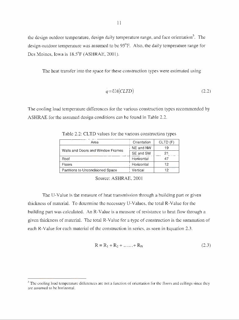
The heat transfer into the space for these construction types were estimated using
q=UA(CLTD) (2.2)
The cooling load temperature differences for the various construction types recommended by
ASHRAE for the assumed design conditions can be found in Table 2.2.
Table 2.2: CLTD values for the various construction types
Area Orientation CLTD (F)
Walls and Doors and Window Frames NE and NW 19
SE and SW 21
Roof Horizontal 47
Floors Horizontal 12
Partitions to Unconditioned Space Vertical 12
Source: ASHRAE, 2001
The U-Value is the measure of heat transmission through a building part or given
thickness of material. To determine the necessary U-Values, the total R-Value for the
building part was calculated. An R-Value is a measure of resistance to heat flow through a
given thickness of material. The total R-Value for a type of construction is the summation of
each R-Value for each material of the construction in series, as seen in Equation 2.3.
(2.3)
5 The cooling load temperature differences are not a function of orientation for the floors and ceilings since they are assumed to be horizontal.

12
For building partitions that are exposed to the outdoor and indoor air, a film resistance for the
inside, Ri, and outside, Ro, must be included to obtain the overall thermal resistance, RT, as
seen in Equation 2.4.
(2.4)
All R-Values for the construction types and inner and outer films were chosen using
ASHRAE recommended values. A wind speed of 7 .5 miles-per-hour (mph) in the summer
was assumed, therefore, value for the outside film resistance of 0.25 (ft2*F*hr)/Btu was used
(ASHRAE, 2001). Using the total R-values for each type of construction the U-value for
each type of construction was determined using
(2.5)
A summary of each U-Value used in the design cooling load calculation can be seen in Table
2.4.
Table 2.3 : U-Values for each construction type for the design cooling load calculations
U-Values - Summer
Building Construction Type U-Value
Notes I Assumptions [Btu/(ft" 2*F*h r)]
Window Frames 0.1940 Frames approx. 5" thick solid wood
Upper Lev. Above Grade Exterior Wall 0.0471 Shingle and insulation portion of wall
Upper Lev. Above Grade Exterior Wall 0.1274 Shingle and stud portion of wall
Upper Lev. Above Grade Exterior Wall 0.0463 Stone and Insulation portion of wall
Upper Lev. Above Grade Exterior Wall 0.1214 Stone and Stud portion of wall
Exposed Floors 0.0965 Concrete and 2" rigid board Insulation
Ceiling 0.0260 Ceiling only - neglect roof A-Value
Doors 0.3817 Doors assumed to be Approx. 2" thick oak wood
Garage Partition 0.0486 Insulation portion of wall
Garage Partition 0.1386 Studded portion of wall
Lower Lev. Above Grade Exterior Wall 0.0641 Insulation and stone exposed in lower level wall
Lower Lev. Above Grade Exterior Wall 0.1616 Studs and stone exposed in lower level
Exterior Wall Between Floors 0.0641 Assumed to be similar to stone insulation wall

13
The total R-Value and U-Value calculations for each construction type for summer
conditions can be seen in Appendix B. In addition, the areas of the various construction
types were calculated by using the blue prints and are tabulated in Appendix A, in Tables A3
through A14. A summary of the cooling loads attributed to these construction types can be
seen in Table 2.3.
Table 2.4: Summary of cooling loads for various construction types
Construction Type Load (MBtuh) Walls above grade 5.59 Walls below grade 0.26 Window Frames 0.74 Ceiling 2.47 Doors 0.29
The individual room loads contributed by each of these construction types can be seen in the
Total Cooling Load Summary in Table 2.5.
Sensible Heat Gain Due to Internal Loads
The internal loads of the residence will consist mainly of occupancy and appliances
that run continuously. The internal heat gain due to lights, bathing, cooking, and laundry
were neglected. These loads could in fact be considered; however, the likelihood of each of
these loads occurring simultaneously and contributing to the block load is minimal and could
lead to over-sizing the equipment.
It was assumed that the occupancy will consist of two adults in the home. Each
person was assumed to contribute an estimated 230 Btuh of sensible heat (ASHRAE, 2001).
For room loads, one occupant was placed in the master bedroom and one in the kitchen on
the upper level.
For the appliances, a refrigerator was included in the kitchen on the upper level and in
the bar area on the lower level. Each refrigerator was assumed to produce roughly 900 Btuh

14
assuming that each refrigerator is approximately 30 cubic feet in volume (ASHRAE, 2001).
The total loads due to the occupancy and appliances were found to be 0.46 and 1.8 MBtuh
respectively. A summary of these loads for each room in the residence can be seen in the
Total Cooling Load Summary section in Table 2.5.
Sensible Heat Gain Due to Infiltration and/or Ventilation
In the early design stages of this project it was decided to use an energy recovery unit
for the circulation of fresh outdoor-air into the home at all times during the use of the heating
and cooling equipment. Further research concluded that an appropriate ventilation rate that is
universally recommended for a new tightly sealed residential home is approximately 0.35 air
changes-per-hour (ACH) (Home Ventilating Institute, 2003). Since outdoor air will be
intentionally introduced into the home while the heating and cooling equipment is in
operation, the home will be put into a more positively pressured state. Therefore, infiltration
through the structure during these times will be decreased ( depending on the outside wind
velocity), however, not eliminated.
For the sensible heat gain due to infiltration and/or ventilation, an ACH value of 0.5
was used as the rate of outdoor air entering the structure. This ACH value is recommended
by ASHRAE for the assumed conditions. This estimated value accounts for both the
ventilation introduced by the heat recovery unit and additional infiltration that may occur
simultaneously on the structure. In addition, this is the recommended infiltration rate given
by ASHRAE for summer conditions and medium6 construction further validating this
assumption. It should be noted that the heat transfer within the heat recovery unit has been
neglected for these calculations and the resulting load estimation will be conservative. The
airflow rate of infiltration and ventilation into the home in units of cubic-feet-per-minute
( cfm) was determined by
6 "Medium" airtightness construction denotes a residential structure that is a new, two-story frame house or onestory house that is more than 10 years old with average maintenance, a floor area greater than 1500 ft2, average fit windows and doors, and a fireplace with damper and glass closure (ASHRAE, 2001).

15
(2.6)
The sensible heat required to cool this amount of air entering the home was calculated
by
(2.7)
Using an airflow rate in units of cfm and standard temperature and pressure, m Cp is reduced
to a value of 1. 1, resulting in heat transfer in units of Btuh. Thus, for the heat transfer in
Btuh equation 2.8 below was used.
q=l.lQ(L1T) (2.8)
The sensible cooling load due to ventilation and infiltration to the home was determined to be
8.04 MBtuh. The load due to ventilation and infiltration for each room in the residence can
be seen in the Total Cooling Load Summary section in Table 2.5.
Latent Heat Gain
The latent heat gain into the structure was found using the ASHRAE recommended
sensible heat factor (SHF) by
q1arenr = (1- SHF) * Total Sensible Load
The sensible heat factor is the ratio of the sensible load to the total load.
SHF = Sensible Load Total Load
(2.9)
(2.10)

16
To determine the total load to the structure accounting for the latent loads, the latent
factor (LF) was used which is the reciprocal of the sensible heat factor.
LF=-1-SHF
Thus, the total design cooling load of the structure was estimated by
q10 1a1 = LF * Total Sensible Load
(2.11)
(2.12)
ASHRAE recommends using a latent factor of 1.3, which is derived from a sensible
heat factor of 0.77, and estimates the performance of a typical residential vapor compression
cooling system (ASHRAE, 2001). However, upon further evaluation, it was determined that
a more accurate representation of the sensible heat factor for the case study home is 0.82.
This result yields a latent factor of 1.22 and was the latent factor used in determining the total
cooling load to the home. The latent load was found to be 9.7 MBtuh.
Total Cooling Load Summary
All contributors to the design cooling load have been evaluated and tabulated in Table
2.5.

Tab
le 2
.5:
Sum
mar
y o
f des
ign
cool
ing
load
cal
cula
tion
s
Tra
ns.
L&
S
HE
AT
MO
DE
S
ensi
ble
(Btu
/hr)
Lo
ad
& S
olar
(B
tu/h
r)
HE
AT
SO
UR
CE
G
lass
W
indo
w
Doo
rs
A. G
. E
xt
Par
t. U
nc.
Cei
ling
Bet
wee
n In
filtr
atio
n P
eopl
e A
pplia
nces
T
otal
(Btu
/hr)
F
ram
e (B
tu/h
r)
Wal
ls
Spa
ce
(Btu
/hr)
F
loor
s (B
tu/h
) (B
tu/h
r)
(Btu
/hr)
Lo
ad
Upp
er L
evel
Roo
m
(Btu
/hr)
(B
tu/h
r)
(Btu
/hr)
(B
tu/h
r)
(Btu
/hr)
Gar
age
0 0
0 0
0 0
0 0
0 0
0 B
ath
off G
araa
e 24
0 17
0
134
42
35
15
53
0 0
654
Ent
rvw
av o
ff G
araa
e 0
0 0
27
29
56
2 85
0
0 24
3 P
antr
v 0
0 0
29
80
83
2 12
5 0
0 39
1 K
itche
n 1,
974
96
121
49
0 32
0 21
48
5 23
0 90
0 5,
118
Sun
room
4,
046
130
0 28
8 0
236
41
358
0 0
6,21
9 D
inin
a R
oom
2,
278
68
0 83
0
216
17
328
0 0
3,64
7 G
reat
-roo
m
3,96
4 61
0
276
0 39
3 27
83
0 0
0 6,
768
Foy
er
1,45
6 17
97
19
8 0
325
26
540
0 0
3,24
2 M
aste
r B
edro
om
2,65
0 93
0
281
0 27
9 43
42
3 23
0 0
4,87
6 H
all o
ff M
aste
r B
ed.
0 0
0 0
0 4
3
0 65
0
0 13
3 B
ath
off M
aste
r B
ed.
943
40
77
276
0 21
3 33
32
2 0
0 2,
322
,__.
Mas
ter
Bed
Clo
set
768
22
0 35
4 0
180
45
273
0 0
2,00
3 --
.J
Laun
drv
Rm
. 0
0 0
0 0
85
0 12
9 0
0 26
1 T
OT
ALS
18
,320
54
4 29
5 1,
996
151
2,46
5 27
3 4,
016
460
900
35,8
77
HE
AT
SO
UR
CE
G
lass
W
ind
ow
C
eilin
g A
. G.
Ext
A
.G. E
xt.
Bet
wee
n E
xpos
ed
Infil
trat
ion
Peo
ple
App
lianc
es
Tot
al
Fra
me
Wal
ls
Wal
ls B
.G.
Flo
ors
Flo
ors
Load
Lo
wer
Lev
el R
oom
(B
tu/h
r)
(Btu
/hr)
(B
tu/h
r)
(Btu
/hr)
(B
tu/h
r)
(Btu
/hr)
(B
tu/h
r)
(Btu
/h)
(Btu
/hr)
(B
tu/h
r)
(Btu
/hr)
Sto
raae
1
0 0
180
0 42
0
-225
25
1 0
0 30
2 S
tora
ge 2
0
0 7
3
0 25
0
-91
102
0 0
132
Gam
e R
oom
0
0 36
6 0
59
0 -4
58
509
0 0
581
Bar
Are
a 0
0 0
0 26
0
-484
53
8 0
900
1,19
6 D
en
1,81
4 53
0
99
37
0 -2
26
314
0 0
2,55
2 S
unke
n R
ec.
Roo
m
5,61
9 56
0
267
0 0
-644
1,
015
0 0
7,69
8 H
all/S
tairs
0
0 0
0 22
0
-204
22
7 0
0 54
M
echa
nica
l R
oom
0
0 0
0 12
0
-81
90
0 26
B
ed 2
2,
185
53
0 38
0 0
0 -3
04
423
0 0
3,33
9 B
ed 3
90
7 33
0
230
39
0 -3
18
443
0 0
1,62
6 B
ath
0 0
0 0
0 0
-99
111
0 0
14
TO
TA
LS
10,5
26
195
619
976
262
0 -3
,134
4,
023
0 90
0 17
,521

18
Design Heating Load Calculation Analysis
The heating loads were calculated in accordance to the recommended ASHRAE
methods. For the heating load calculations, the heat lost through the structure in each room
per hour for design conditions in the winter was estimated and then summed to attain the
design heating load. Typically, the design heating load is estimated for conditions in the
middle of the night during the winter time when outside air humidity levels are low;
therefore, the heating loads will only account for sensible heat transmission. It was assumed
that the moisture levels in the home during the winter will be maintained through the
occupancy, bathing, cooking, and laundry.
Sensible Heat Loss through Envelope Components
The design sensible heat losses through the glass, walls, window frames, doors,
ceilings, and floors were estimated by using the overall heat transfer coefficient, its area, and
the relevant temperature difference across the construction type. The design outdoor-air and
indoor-air temperature for the design heating load calculations were assumed to be -9°F and
68°F respectively. Further, it should be noted that the estimation of the heating load for these
construction types only accounts for heat transmission losses and neglects any heat gain due
to solar loads. This approach was taken assuming that the maximum heating load will occur
on the home in the winter time and during the middle of the night when the sun is down,
thus, solar gain is irrelevant.
The estimation of the heat loss through each construction type was determined using
(2.13)
The approach for the determination of the U-Values for each construction type was
calculated in the same manner as for the cooling loads assuming that the thermal conductivity
of the building envelope is constant with changing temperature. The outside film resistance

19
under the winter conditions is different from summer conditions, and it is due to a different
assumed wind speed. The design wind speed in the winter was assumed to be 15 mph, thus,
changing the recommended outside film resistance, Ro, from 0.25 to 0.17 (ft2*F*hr)/Btu
(ASHRAE, 2001). All U-Values under the winter conditions were calculated and can be
seen in Table 2.6.
Table 2.6: U-Values for each type of construction for the heating load calculations
Li-Values - Winter
Building Construction Type Li-Value
Notes I Assumptions [Btu/(ft/'2*F*hr)]
Window Frames 0.1970 Frames approx. 5" thick solid wood
Upper Lev. Above Grade Exterior Wall 0.0473 Shingle and insulation portion of wall
Upper Lev. Above Grade Exterior Wall 0.1287 Shingle and stud portion of wall
Upper Lev. Above Grade Exterior Wall 0.0465 Stone and Insulation portion of wall
Upper Lev. Above Grade Exterior Wall 0.1226 Stone and Stud portion of wall
Exposed Floors 0.0965 Concrete and 2" rigid board Insulation
Ceiling 0.0260 Ceiling only - neglect roof R-Value
Doors 0.3937 Doors assumed to be Approx. 2" thick oak wood
Garage Partition 0.0486 Insulation portion of wall
Garage Partition 0.1386 Studded portion of wall
Exterior Wall Between Floors 0.0644 Assumed to be similar to stone insulation wall
Glass 0.3200 Double pane, Low-E, Argon filled, interior shading
All R-Values with the exception of the glass values were attained as per ASHRAE
recommendations. The U-Value for the glass was obtained directly from the glass
manufacturer, and was found to be 0.32 Btu/(ft2*F*hr). This U-Value was determined
knowing that the windows are double pane windows with a Low-E coating and filled with
argon gas.
The areas for each type of construction were determined from the blueprints and can
be found in Tables Al through A14 in Appendix A. Finally, all of the design heating loads
for the previously mentioned construction types were estimated using Equation 2.13 and a
summary of these loads can be seen in Table 2. 7.

20
A summary of the loads contributed by each of these construction types for each room can be
seen in the Total Heating Load Summary section in Table 2.8.
Table 2.7: Summary of design heating loads for various construction types
Construction Type Load (MBtuh) Glass 18.3 Walls 18.0 Window Frames 2.8 Ceiling 3.5 Floors 5.8 Doors 1.2
Sensible Heat Gain Due to Internal Loads
The internal loads consist mainly of occupancy and appliances that run continuously,
similarly to the cooling loads. However, the internal loads for the heating calculations will
actually contribute to heating the space and will reduce the load on the heating equipment.
The internal heat gain due to lights, bathing, cooking, and laundry were again neglected
because the peak heating load was assumed to occur in the middle of the night when
occupants are most likely asleep.
It was assumed for the design heating load that the occupancy consists of two adults
in the home. It was assumed that each person will emit approximately 230 Btuh of sensible
heat into the space (ASHRAE, 2001). For room loads, one occupant was placed in the
master bedroom and one in the kitchen on the upper level.
For the appliances, a refrigerator was included in the kitchen on the upper level and in
the bar area on the lower level. Each refrigerator was assumed to contribute roughly 900
Btuh, assuming that each refrigerator is approximately 30 cubic feet in volume (ASHRAE,
2001). A summary of these loads for each room in the residence can be seen in the Total
Heating Load Summary section in Table 2.8.

21
Sensible Heat Loss Due to Infiltration and/or Ventilation
Again, the ACH method was used to estimate the heat loss due to infiltration and
ventilation for the heating load. The assumed flow rate of air entering the home was again
0.5 air changes per hour. The sensible heat lost due to infiltration was determined using
Equation 2.8. The contribution of the ventilation and infiltration to the total design heating
load was found to be 26.6 MBtuh. The load due to ventilation and infiltration for each room
in the residence can be seen in the Total Heating Load Summary section in Table 2.8.
Total Heating Load Summary
All of the estimated heating loads per room and for the entire home can be seen in
Table 2.8.

HE
AT
MO
DE
T
ran
s.
& S
ola
r
HE
AT
SO
UR
CE
W
ind
ow
G
lass
(B
tu/h
r)
Fra
me
Up
pe
r Le
vel
(Btu
/hr)
Ba
th o
ff G
ara
ge
1
85
6
8
En
trvw
av
off
Ga
raq
e
0 0
Pa
ntr
y 0
0 K
itch
en
1
,52
0
39
7
Su
nro
om
2,
723
50
8
Din
inq
Roo
m
1,36
1 25
4 G
rea
t-ro
om
2
,36
9
226
Fo
yer
1,12
1 7
0
Ma
ste
r B
edro
om
1,5
83
34
5 H
all
off
Ma
ste
r B
ed
0 0
Ba
th o
ff M
ast
er
Bed
. 56
4 15
1 C
lose
t o
ff M
ast
er
Bed
59
1 91
L
au
nd
ry R
oom
0
0 T
OT
AL
S
12
,01
7
2,1
09
HE
AT
SO
UR
CE
W
ind
ow
G
lass
F
ram
e
Low
er L
evel
(B
tu/h
r)
(Btu
/hr)
Sto
raq
e 1
0
0 S
tora
ge
2
0 0
Ga
me
Roo
m
0 0
Ba
r A
rea
0
0 D
en
1
,08
4
19
7
Su
nke
n R
ec.
Roo
m
3,3
57
2
09
H
all
0 0
Me
cha
nic
al
Roo
m
0 0
Be
d 2
1
,30
6
19
7
Be
d 3
54
2 12
1 B
ath
0
0 T
OT
AL
S
6,2
89
72
4
Tab
le 2
.8:
Sum
mar
y o
f des
ign
heat
ing
load
cal
cula
tion
s
Se
nsi
ble
A.G
. E
xt
Par
t. U
nc.
E
xpo
sed
D
oo
rs
Ce
ilin
g
Infil
tra
tion
(B
tu/h
r)
Wa
lls
Sp
ace
(B
tu/h
r)
Flo
ors
(B
tu/h
) (B
tu/h
r)
(Btu
/hr)
(B
tu/h
r)
0 5
16
2
70
5
0
0 2
25
0
111
184
80
0
35
7
0 1
08
5
16
1
18
0
52
7
50
6
201
0 4
57
0
2,0
40
0
1,13
1 0
33
7
0 1
,50
4
0 3
08
0
30
8
0 1
,37
7
0 1,
031
0 5
60
0
3,4
88
40
4 84
5 0
463
0 2
,27
0
0 1
,03
7
0 3
98
0
1,7
78
0
0 0
62
0
27
5
291
1,04
5 0
30
3
0 1
,35
3
0 1
,62
6
0 2
57
0
1,1
49
0
0 0
121
0 54
1 1,
201
7,9
59
9
70
3
,51
4
0 1
6,8
85
A.G
. Ext
B
.G.
Ext
. E
xpo
sed
B
etw
ee
n
Do
ors
W
alls
W
alls
F
loo
rs
Flo
ors
In
filtr
atio
n
(Btu
/hr)
(B
tu/h
r)
(Btu
/hr)
(B
tu/h
r)
(Btu
/hr)
(B
tu/h
)
0 0
66
4
33
0
13
9
12
0
0 0
38
0
13
4
82
4
9
0 0
771
671
18
9
244
0 0
475
70
9
84
25
7
0 3
66
5
93
5
08
2
03
1,
321
0 9
94
0
1,44
9 1
64
4,
268
0 0
30
8
29
9
69
9
53
0
0 1
90
1
19
40
43
0
1,4
03
0
684
19
8
1,7
79
0
871
59
3
71
6
248
21
2
0 0
0 14
6 0
46
5
0 3
,63
3
3,97
4 5
,76
5
1,4
16
9
,71
0
Pe
op
le
Ap
plia
nce
s (B
tu/h
r)
(Btu
/hr)
0 0
0 0
0 0
-23
0
-90
0
0 0
0 0
0 0
0 0
-23
0
0 0
0 0
0 0
0 0
0 -4
60
-90
0
Pe
op
le
Ap
plia
nce
s (B
tu/h
r)
(Btu
/hr)
0 0
0 0
0 0
0 -9
00
0
0 0
0 0
0 0 0
0 0
0 0
0 0
-90
0
Se
nsi
ble
(B
tu/h
r)
Tot
al
Se
nsi
ble
L
oa
d
(Btu
/hr)
1
,31
4
73
2
1,2
69
3
,99
0
6,2
03
3
,60
9
7,6
73
5
,17
3
4,91
2 3
37
3
,70
6
3,7
14
6
62
43
,294
T
ota
l S
en
sib
le
Lo
ad
(B
tu/h
r)
1,25
4 6
44
1
,87
4
62
6
4,2
74
1
0,4
40
1
,62
9
39
2
5,5
67
3
,30
3
611
30
,61
4
N
N

23
CHAPTER 3 - HEATING AND COOLING ALTERNATIVE APPROACHES
Several alternative approaches for heating and cooling the home with the geothermal
and radiant floor systems are presented within this section. Subsequently, through evaluation
of cost, availability, installation, and control flexibility specifics of each alternative, the best
available system was chosen for the home. Using geothermal and radiant floor systems, the
following approach for conditioning the home was developed, seen in Table 3.1.
Table 3.1: Heating and cooling approach 1
APPROACH 1 HEATING COOLING
Upper Level Forced Air - GSHP Air Heating Forced Air - GSHP Air Cooling
Lower Level Radiant Floor - GSHP Hydronic Heating Forced Air - GSHP Air Cooling
Garage Radiant Floor - GSHP Hydronic Heating None
The possibility of a hybrid system was also considered. Initial research performed as
part of this study along with lengthy discussion with two independent subcontractors
suggested that using a geothermal approach for the radiant floor heating may be
uneconomical in the long run. This suggestion was based on the requirement of additional
wells and the required use of more expensive equipment. Further, by using the same loop
field for two heat pumps, additional system design, pumps, valves, and controls would be
necessary. Therefore, the following two approaches were developed using conventional
methods for the radiant floor in conjunction with geothermal means for the forced air heating
and cooling. Approach 2 (Table 3.2) utilizes an electric boiler for hydronic heating to the
radiant floor.
Table 3.2: Heating and cooling approach 2
APPROACH 2 HEATING COOLING
Upper Level Forced Air - GSHP Air Heating Forced Air - GSHP Air Cooling Lower Level Radiant Floor - Electric Boiler Forced Air - GSHP Air Cooling Garage Radiant Floor - Electric Boiler None
24
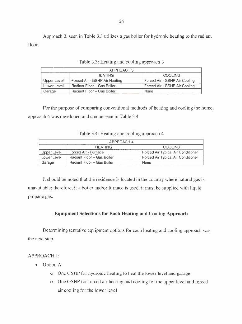
Approach 3, seen in Table 3.3 utilizes a gas boiler for hydronic heating to the radiant
floor.
Table 3.3: Heating and cooling approach 3
APPROACH 3 HEATING COOLING
Upper Level Forced Air - GSHP Air Heating Forced Air - GSHP Air Cooling
Lower Level Radiant Floor - Gas Boiler Forced Air - GSHP Air Cooling
Garage Radiant Floor - Gas Boiler None
For the purpose of comparing conventional methods of heating and cooling the home,
approach 4 was developed and can be seen in Table 3.4.
Table 3.4: Heating and cooling approach 4
APPROACH 4 HEATING COOLING
Upper Level Forced Air - Furnace Forced Air Typical Air Conditioner Lower Level Radiant Floor - Gas Boiler Forced Air Typical Air Conditioner Garage Radiant Floor - Gas Boiler None
It should be noted that the residence is located in the country where natural gas is
unavailable; therefore, if a boiler and/or furnace is used, it must be supplied with liquid
propane gas.
Equipment Selections for Each Heating and Cooling Approach
Determining tentative equipment options for each heating and cooling approach was
the next step.
APPROACH 1:
• Option A:
o One GSHP for hydronic heating to heat the lower level and garage
o One GSHP for forced air heating and cooling for the upper level and forced
air cooling for the lower level

25
• Option B:
o One GSHP for hydronic heating for the lower level and garage and forced air
heating for the upper level and forced air cooling to the upper and lower level
APPROACH 2:
• Option A:
o One GSHP for forced air heating and cooling for the upper level and forced
air cooling for the lower level
o One electric resistance boiler for hydronic heating to the lower level and
garage
APPROACH 3:
• Option A:
o One GSHP for forced air heating and cooling for the upper level and forced
air cooling for the lower level
o One gas boiler for hydronic heating to the lower level and garage
APPROACH 4:
• Option A:
o One gas furnace for forced air heating to the upper level
o One standard air conditioner for forced air cooling the upper and lower level
o One gas boiler for hydronic heating to the lower level and garage
The estimated heating and cooling loads that were previously determined for the
upper and lower level and garage will be the demand that the equipment must meet in order
to maintain a comfortable environment in the home under the assumed design conditions, and
can be seen in Table 3.5.
26
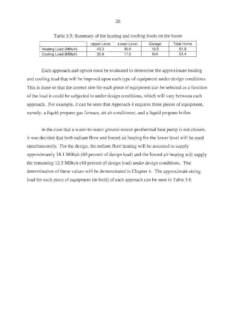
Table 3.5: Summary of the heating and cooling loads on the home
Upper Level Lower Level Garage Total Home
Heating Load (MBtuh) 43.3 30.6 18.0 91.9 Cooling Load (MBtuh) 35.9 17.5 N/A 53.4
Each approach and option must be evaluated to determine the approximate heating
and cooling load that will be imposed upon each type of equipment under design conditions.
This is done so that the correct size for each piece of equipment can be selected as a function
of the load it could be subjected to under design conditions, which will vary between each
approach. For example, it can be seen that Approach 4 requires three pieces of equipment,
namely: a liquid propane gas furnace, an air conditioner, and a liquid propane boiler.
In the case that a water-to-water ground-source geothermal heat pump is not chosen,
it was decided that both radiant floor and forced air heating for the lower level will be used
simultaneously. For the design, the radiant floor heating will be assumed to supply
approximately 18.1 MBtuh (60 percent of design load) and the forced air heating will supply
the remaining 12.5 MBtuh (40 percent of design load) under design conditions. The
determination of these values will be demonstrated in Chapter 4. The approximate sizing
load for each piece of equipment (in bold) of each approach can be seen in Table 3.6.
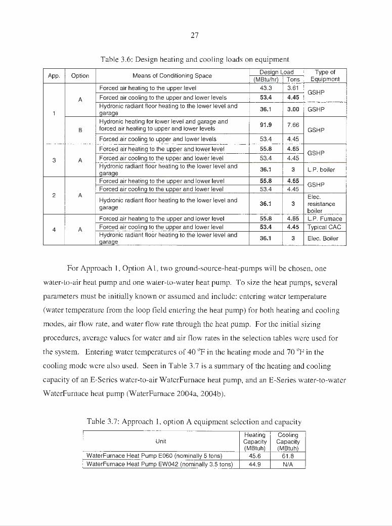
27
Table 3.6: Design heating and cooling loads on equipment
App. Option Means of Conditioning Space Design Load Type of
(MBtu/hr) Tons Equipment
Forced air heating to the upper level 43.3 3.61 GSHP
A Forced air cooling to the upper and lower levels 53.4 4.45 Hydronic radiant floor heating to the lower level and 36.1 3.00 GSHP
1 qaraqe
Hydronic heating for lower level and garage and 91.9 7.66 B forced air heating to upper and lower levels GSHP
Forced air cooling to upper and lower levels 53.4 4.45
Forced air heating to the upper and lower level 55.8 4.65 GSHP
3 A Forced air cooling to the upper and lower level 53.4 4.45 Hydronic radiant floor heating to the lower level and 36.1 3 L.P. boiler qaraqe Forced air heating to the upper and lower level 55.8 4.65
GSHP Forced air cooling to the upper and lower level 53.4 4.45
2 A Elec. Hydronic radiant floor heating to the lower level and 36.1 3 resistance garage
boiler Forced air heating to the upper and lower level 55.8 4.65 L.P. Furnace
4 A Forced air cooling to the upper and lower level 53.4 4.45 Typical CAC Hydronic radiant floor heating to the lower level and 36.1 qaraqe 3 Elec. Boiler
For Approach 1, Option Al, two ground-source-heat-pumps will be chosen, one
water-to-air heat pump and one water-to-water heat pump. To size the heat pumps, several
parameters must be initially known or assumed and include: entering water temperature
( water temperature from the loop field entering the heat pump) for both heating and cooling
modes, air flow rate, and water flow rate through the heat pump. For the initial sizing
procedures, average values for water and air flow rates in the selection tables were used for
the system. Entering water temperatures of 40 °F in the heating mode and 70 °F in the
cooling mode were also used. Seen in Table 3.7 is a summary of the heating and cooling
capacity of an E-Series water-to-air Water Furnace heat pump, and an E-Series water-to-water
WaterFurnace heat pump (WaterFurnace 2004a, 2004b).
Table 3.7: Approach 1, option A equipment selection and capacity
Heating Cooling Unit Capacity Capacity
(MBtuh) (MBtuh) WaterFurnace Heat Pump E060 (nominally 5 tons) 45.6 61.8 WaterFurnace Heat Pump EW042 (nominally 3.5 tons) 44.9 N/A

28
It can be seen that the total heating capacity of the nominal 5 ton water-to-air and the
nominal 3.5 ton water-to-water heat pump is approximately 90.5 MBtuh. The design heat
loss to the home is 73.9 MBtuh; using these heat pumps, under design conditions, the heating
capacity left for the garage is approximately 16.6 MBtuh. Assuming that the design heat loss
to the garage is 18.0 MBtuh (at an indoor air temperature of 50 °F), the system would be able
to heat the garage to approximately 45°F, resulting in an acceptable tentative option.
The match of the cooling capacity to the design demand would be acceptable. Using
the nominal 5 ton unit on high speed the cooling capacity is about 8.4 MBtuh oversized. A
little over-sizing is acceptable in this situation due to the duel speed capability and for pick
up of the space temperature.
For Approach 1, option B, one heat pump can be used. WaterFurnace's Synergy 3
unit has the capability of heating either water or air in the same mode and cooling air. This
unit is fairly new on the market and was considered with caution. The heating capacity for
both the water and air and cooling capacity for the air can be seen in Table 3.8.
Table 3.8: Approach 1, option B equipment selection and capacity
Air Heating Water Heating Air Cooling Unit Capacity Capacity Capacity
(MBtuh)* (MBtuh)* (MBtuh) WaterFurnace Heat Pump RTV066 60 44.2 64.6
* Unit can heat either air or water in the same mode
The heating capacity of this unit on the air side is approximately 60.0 MBtuh, which
falls short of the design heating demand. However, the electric resistance auxiliary heating
would be available to make up the remainder of the load. The cooling capacity of this unit in
comparison to the design heat gain is acceptable.
Approach 2, option A would essentially replace the water-to-water heat pump with an
electric boiler. The specific equipment information for this approach can be seen in Table
3.9.

29
Table 3.9: Approach 2, option A equipment selection and capacity
Heating Cooling Unit Capacity Capacity
(MBtuh) (MBtuh) WaterFurnace Heat Pump E060 45.6 61.8 Thermolec Electric Resistance Boiler 78.43 (15 KW) N/A
Approach 3, option A, includes a water-to-air heat pump used with a Weil McLain
Ultra 105 MBtuh propane fired hydronic boiler. Using the nominal 5 ton heat pump with the
boiler will provide adequate capacity for both heating and cooling. The equipment capacity
can be seen in Table 3.10.
Table 3.10: Approach 3, option A equipment selection and capacity
Heating Cooling Unit Capacity Capacity
(MBtuh) (MBtuh) WaterFurnace Heat Pump E060 45.6 61 .8 Weil McLain Ultra 105 Boiler 105 N/A
Finally, approach 4, option A was considered and quoted by the contractor. This
option was based entirely on conventional methods of heating and cooling a home and was
included in this analysis as a baseline for comparison to the other approaches. This option
consists of a liquid propane fired furnace and boiler, and a typical vapor compression
refrigeration cycle air conditioner.
Table 3.11: Approach 4, option A equipment selection and capacity
Heating Cooling Unit Capacity Capacity
(MBtuh) (MBtuh) Bryant Gas Furnace 92% Model# 340MA V0600120 120.0 N/A Bryant 5 TON 12 S.E.E.R. Air Conditioner N/A 60.0 Weil McLain L.P. Ultra 105 Boiler 105.0 N/A
This system will easily meet both the heating and cooling demand of the home under
design conditions. However, the heating and capacity of the system is in great excess of the
estimated design loads.

30
CHAPTER 4 - ANNUAL ENERGY USE AND HVAC OPERATING
PERFORMANCE MODEL
The model presented herein estimates monthly and annual energy use of the residence
by executing an hourly simulation of the relevant energy transfers. This method is based on
an energy balance and considers transmission, solar, infiltration, and internal loads on the
home. A diagram showing each of the considered energy transfers can be seen in Figure 4.1.
qtransmission
Toutdoor
qinfiltration ---~~
Figure 4.1: Energy flows to and from the home
For obtaining weather data for estimating hourly loads (i.e., transmission, infiltration
and solar) to the home, Typical Meteorological Year (TMY2) data was used. TMY2 data is a
set of hourly values of solar and meteorological elements for a location over a one-year
period. This data is intended for computer simulations of solar energy conversion systems
and building systems to facilitate performance comparisons of different system types,
configurations, and locations in the United States. Because TMY2 data represents typical
rather than extreme conditions, they are not suited for designing systems to meet the worst
case conditions occurring at a location (NREL, 1995).
From the previous sections of the study, it was determined that both a forced air
distribution system and a radiant floor system will be used to heat the home. The lower level
of the home will be heated by both systems, and it will be necessary to know the heating

31
loads for each level and garage separately to determine the amount of energy demanded by
each system. Therefore, the following analysis for heating was performed by estimating the
hourly heating loads for the upper level, lower level and garage, separately. With these
results, the hourly demand on each system and hourly cost of each system in the heating
mode was determined.
The cooling of the home will be supplied by the forced air distribution system
exclusively. Therefore, the analysis of the cooling loads was performed by determining the
upper and lower level hourly heat gain together and the garage was excluded since it will not
be cooled. With these results, the respective hourly costs for cooling the home with the
forced air distribution were determined.
Transmission Heat Gain and Loss
Transmission heat transfer to and from each part of the home is driven by conduction
and will occur when there is a temperature difference between the indoor and outdoor air.
For the hourly simulation of transmission heat transfer, outdoor-air dry-bulb temperatures
from the TMY2 data were used. Also, constant indoor-air dry-bulb temperatures were
assumed; the indoor air temperature for the upper and lower levels for heating was assumed
to be 68°F and 50°F for the garage, respectively. Further, an indoor air temperature of 75°F
for the upper and lower levels was assumed for the cooling mode. The hourly transmission
heat transfer to and from the home through the walls, windows, etc. are assumed to be one
dimensional conduction heat transfer and were estimated by
Heating: q transmission , i = UAconduction (T;ndoor air - T outdoor air,i ) (4.1)
Cooling: q transmission, i = UAconduction (Toutdoor air,i - 'I;ndoor air ) (4.2)
where the subscript i represents each hour of the year.

32
The UAconduction term is the combined thermal transmittance of the home and
represents the amount of energy conducted through the structure per unit time per unit of
temperature, e.g., Btu's per hour per degree Fahrenheit [Btu/(hr*F)]. The UAconduction value is
found by
UAejfective = U wall !Awalll + U wall2 A wal/2 + ········ ··· + U walli A walli
+ U window ]Awindow l + U window2 A window2 + ........... + u windowi A windowi
+ U door ! A door l + U door2 A door2 + ··········· + U doori A doori
(4.3)
+Ux! A x l +Ux2 A x2 + ..... . ..•.. +Uxi A xi
The subscript x in Equation 4.3 represents any other structural component that would be
subjected to conduction energy transfer, e.g. , ceiling, exposed floor, etc. This value was
determined using the blueprints for the home and for both summer and winter conditions.
The UAconduction value calculated for a heating condition was 0.3606 MBtu/(hr*F) for the
upper level, 0.3011 MBtu/(hr*F) for the lower level and 0.1695 MBtu/(hr*F) for the garage.
The UAconduction value calculated for a cooling condition was 0.703 MBtu/(hr*F) for the entire
home.
Infiltration Heat Gain and Loss
Infiltration is the uncontrolled movement of outdoor air into the building through
cracks, windows, doors and other openings in the building envelope. The amount of
infiltration occurring at a particular time can be mainly attributed to the structure tightness,
wind speed, wind direction and outdoor air temperature. To estimate infiltration loads for
each level and to the garage of the home, correlations developed by ASHRAE were used.
These correlations estimate infiltration air changes per hour (ACH) under particular
conditions. The air change per hour value represents the number of times the air in the home
is completely replaced by outdoor air via infiltration.

33
Table 4.1: Winter air exchange rates
Class Outdoor Air Temperature (F'
50 40 30 20 10 0 -10 -20 -30 -40 Tight 0.41 0.43 0.45 0.47 0.49 0.51 0.53 0.55 0.57 0.59 Medium 0.69 0.73 0.77 0.81 0.85 0.89 0.93 0.97 1 1.05 Loose 1 .11 1.15 1.2 1.23 1.27 1.3 1.35 1.4 1.43 1.47
Source: ASHRAE, 2001
The winter design air exchange rate values assume an outdoor air wind speed of 15
miles per hour (ASHRAE, 2001). The values in Table 4.1 were plotted and lines were fit to
the data to obtain the ACH as a function of outdoor air temperature in equation form.
Winter Air Exchange Rates (ACH) as a Function of Airtightness
• Tight Construction
:c u 0.8 • Medium Construction <(
• Loose Construction 0.6
0.4
0 .2
0
-40 ·30 ·20 -10 0 10 20 30 40 50
Outdoor Air Temperature (F)
Figure 4.2: Winter design ACH values
The fitted equation for a tight construction home for ACH as a function of outdoor air
temperature was found to be
ACH W int er, ; = -0.002(OATJ+ 0.51 (4.4)
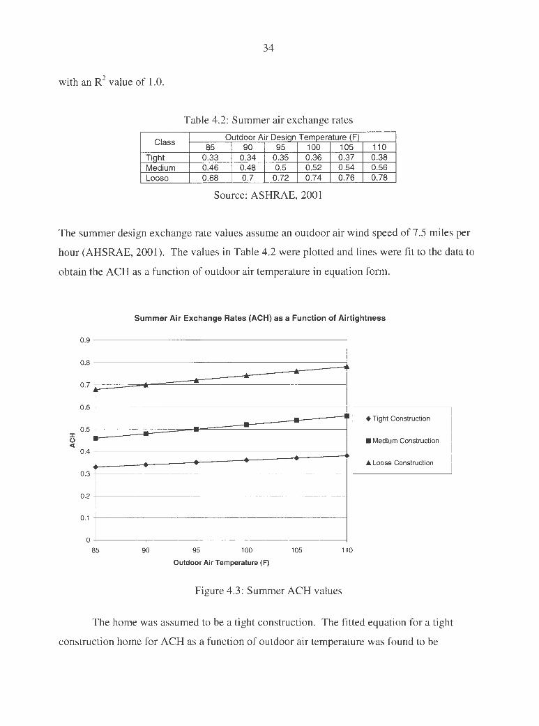
34
with an R2 value of 1.0.
Table 4.2: Summer air exchange rates
Class Outdoor Air Desiqn Temperature (F)
85 90 95 100 105 110 Tiqht 0.33 0.34 0.35 0.36 0.37 0.38 Medium 0.46 0.48 0.5 0.52 0.54 0.56 Loose 0.68 0.7 0.72 0.74 0.76 0.78
Source: ASHRAE, 2001
The summer design exchange rate values assume an outdoor air wind speed of 7.5 miles per
hour (AHSRAE, 2001). The values in Table 4.2 were plotted and lines were fit to the data to
obtain the ACH as a function of outdoor air temperature in equation form.
Summer Air Exchange Rates (ACH) as a Function of Airtightness
0.9
0.8 ~
--0.7 --.. 0.6 ... -- - • Tight Construction
0 .5 - -- -J: -u ,r-<(
• Medium Construction
0.4 £
~ - ~ • Loose Construction
0.3
0.2
0.1
0
85 90 95 100 105 110
Outdoor Air Temperature (F)
Figure 4.3: Summer ACH values
The home was assumed to be a tight construction. The fitted equation for a tight
construction home for ACH as a function of outdoor air temperature was found to be

35
ACH Summer,; = 0.002(OAT; )+0.16 (4.5)
with an R2 value of 1.0.
For simulating the infiltration for each hour of the year, the ACH values were
adjusted according to the wind speed and outdoor air temperature. The phenomenon of
infiltration is driven by a pressure difference across the building shell, which is caused by the
pressure exerted by the wind on the exterior walls of the home. These pressures arise from
the conversion of the kinetic energy of the wind into a pressure rise against the wall as the air
is brought to rest, or stagnation (Munson, Young, & Okiishi, 2002). A diagram of the
pressure rise on the exterior walls of the home assuming that the indoor air pressure is equal
to the atmospheric air pressure can be seen in Figure 4.3.
Outdoors Indoors
Wind
(l )• (2) •
Pann
Figure 4.4: Diagram of wind pressure on exterior walls of the home
The pressure rise from atmospheric pressure to P2 can be estimated by the Bernoulli
equation assuming that the air acts as an incompressible fluid at the relatively low velocities
that could typically be expected with wind.
p = p + v a:r . 2 atm 2 P air (4.6)

36
Rewriting this equation in terms of a change in pressure across the partition assuming that the
indoor air pressure is equal to atmospheric pressure yields
M p p V a~r = 2 - atm =2 P air (4.7)
Thus, the pressure difference across the exterior wall is proportional to the velocity squared
assuming that the wind is perpendicularly striking the wall.
(4.8)
Assuming that all doors and windows are closed, the air will be entering the home primarily
through cracks in the walls. These cracks in the home were modeled as a single orifice, seen
in Figure 4.5 .
Figure 4.5: Diagram of air infiltrating through a wall crack
The volumetric flow rate of air entering the home through the cracks can be represented as
Q=VA (4.9)
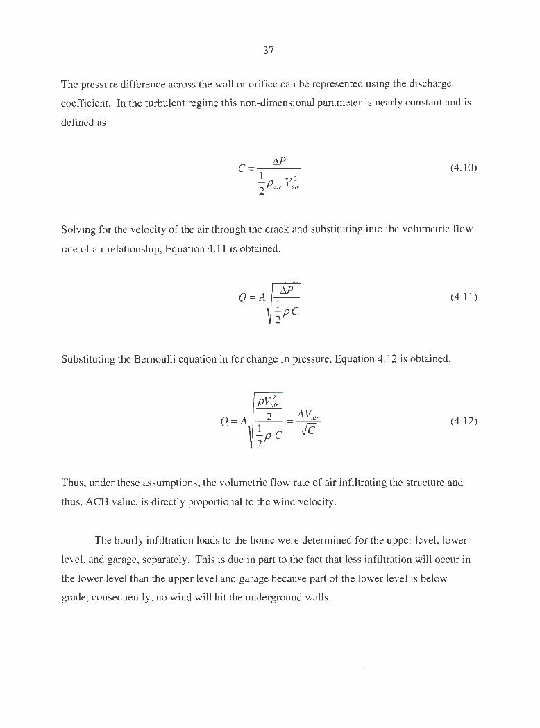
37
The pressure difference across the wall or orifice can be represented using the discharge
coefficient. In the turbulent regime this non-dimensional parameter is nearly constant and is
defined as
C= M 1 2
2P air V air
(4.10)
Solving for the velocity of the air through the crack and substituting into the volumetric flow
rate of air relationship, Equation 4.11 is obtained.
(4.11)
Substituting the Bernoulli equation in for change in pressure, Equation 4.12 is obtained.
Q=A (4.12)
Thus, under these assumptions, the volumetric flow rate of air infiltrating the structure and
thus, ACH value, is directly proportional to the wind velocity.
The hourly infiltration loads to the home were determined for the upper level, lower
level, and garage, separately. This is due in part to the fact that less infiltration will occur in
the lower level than the upper level and garage because part of the lower level is below
grade; consequently, no wind will hit the underground walls.

38
To estimate the hourly ACH for the upper level and garage, hourly wind values and
outdoor-air dry-bulb temperatures were used from the TMY2 data. The ACH values were
estimated using Equations 4.4 and 4.5 and prorated according to the wind speed at the
particular hour. For example, in the summer or cooling mode the ACH value was estimated
to be 1.02 for a "tight" class home and an outdoor-air dry-bulb temperature of 90°F and wind
speed of 22.5 miles per hour.
The estimation of the ACH of the lower level was made considering that part of the
lower level is below grade. The lower level of the case study residence has exposed walls
only on the southeast and southwest sides. Therefore, it was assumed that the ACH of the
lower level is zero when the wind was blowing between the directions north of east and west
of southwest. During the hours when the wind is blowing at all other directions, the ACH of
the lower level was estimated to be the same as for the upper level and garage.
Once the hourly ACH values were estimated for each part of the home, the energy
required to heat or cool the air in Btu ' s per hour was determined by
H t. . · _ 1.08 * ACH; * (Zone Volume) * (T;ndoorair -Toutdoorair,i )(wsi ) ea mg. q.nf .1 . . - - -
1 , tratwn,, 60 15 (4.13)
C r . . _ 1.I * ACH;* (ZoneVolume) * (Toutdoorair,i -Tindoorair )(wsi) 00 mg. qinf iltration,i - 60 7.5 (4.14)
where the zone volume represents the volume of the upper level, lower level or garage. It
should be noted that the volume is in cubic feet and the temperatures are in degrees
Fahrenheit.
Solar Heat Gain
The total solar radiation striking the home can be split into two components, beam
and diffuse radiation. The beam radiation is the solar radiation striking the home from the

39
sun without having been scattered by the atmosphere and it is often referred to as direct solar
radiation (Duffy & Beckman 1991). The diffuse radiation is the solar radiation striking the
home from the sun after its direction has been changed due to scattering by the atmosphere,
and it is often referred to as solar sky radiation (Duffy & Beckman 1991). Thus, the total
irradiance, which is the rate at which radiant energy is incident on a surface per unit area of
surface, is the sum of the beam and diffuse radiation rates per unit area.
The TMY2 data gives solar values for a horizontal surface; therefore, the amount of
solar radiation incident on a vertical surface, e.g., the windows, must be found. The hourly
beam radiation incident on a tilted surface can be determined by
The parameter Rb represents the ratio of beam radiation on a tilted surface to that on a
horizontal surface for a particular hour and was determined by
cos(e);
cos(02 \
(4.15)
(4.16)
The angle of incidence, 0, is the angle between the beam radiation on a surface and the
normal to that surface; whereas, the zenith angle, 02 , is the angle between the vertical and the
line to the sun. The angle of incidence and the zenith angle were determined by
cos(e); = sin(o); sin(¢)cos(,B)
-sin(o); cos(¢)sin(,B)cos(r)
+ cos(o); cos(¢)cos(,B)cos(m);
+ cos(J); sin(¢ )sin(,B)cos(y )cos(m);
+cos(o); sin(,B)sin(y)sin(m);
cos(02 ) ; = cos(¢)cos(5); cos(m); + sin(¢)sin(5);
( 4.17)
(4.18)
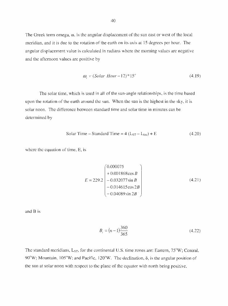
40
The Greek term omega, ffi, is the angular displacement of the sun east or west of the local
meridian, and it is due to the rotation of the earth on its axis at 15 degrees per hour. The
angular displacement value is calculated in radians where the morning values are negative
and the afternoon values are positive by
OJ; = (Solar Hour-12) * 15° (4.19)
The solar time, which is used in all of the sun-angle relationships, is the time based
upon the rotation of the earth around the sun. When the sun is the highest in the sky, it is
solar noon. The difference between standard time and solar time in minutes can be
determined by
Solar Time - Standard Time = 4 (LsT - L1oc) + E
where the equation of time, E, is
and Bis
0.000075
+ 0.001868cosB
E = 229.2 - 0.032077 sin B
-0.014615cos2B
- 0.04089 sin 2B ·
B. =(n-1)360 l 365
(4.20)
(4.21)
(4.22)
The standard meridians, LsT, for the continental U.S. time zones are: Eastern, 75°W; Central,
90°W; Mountain, 105°W; and Pacific, 120°W. The declination, 8, is the angular position of
the sun at solar noon with respect to the plane of the equator with north being positive.

41
<5 = 23.45 * sin(360 284 + n) I 365
(4.23)
The latitude, <p, for the case study home was determined using a global positioning system
(GPS) to be 42 degrees. In addition, all windows of the home are oriented vertically;
therefore, the slope of each surface, p, is 90 degrees. The surface azimuth angle, y, is the
deviation of the projection on a horizontal plane of the normal to the surface from the local
meridian, with zero due south, east negative, and west positive (Duffy & Beckman 1991).
This value was also determined using a GPS device. The back of the home faces southwest,
resulting in a surface azimuth of 45 degrees.
Any beam insolations that were calculated and corresponded to a negative cos(0) or
cos(02) were set to zero. This was done because negative values for these parameters indicate
that either the sun has gone under the horizon or the sun is behind the surface so that there is
no incident beam radiation on the window face .
The hourly diffuse radiation on a tilted surface was determined by
1 = 1 ( 1 + cos(/J)) + / ·( 1- cos(/J)) d,T d 2 Pg, , 2
(4.24)
The ground reflectance, pg, was estimated assuming two conditions, grass and snow covered.
The hourly snow depth values from the TMY2 data were used to determine if the ground was
snow covered. If the snow depth for the hour was found to be greater than zero, then the
ground reflectance was assumed to be 0.7; otherwise, the ground was assumed to be grass
covered with an approximate ground reflectance value of 0.25. All of the hourly diffuse
values that corresponded to a negative cos(02) value were set to zero.
The total amount of solar energy entering the home through the glass is a function of
the solar heat gain coefficient (SHGC) of the glazing and the type of interior shading. The

42
SHGC is the fraction of incident solar radiation admitted through a window, both directly
transmitted and absorbed, and then subsequently released into the home (ASHRAE, 2001).
The SHGC for a window is a function of the angle of incidence of the solar radiation. For
this study, the program WINDOW 5.1 was used to determine the SHGC of the windows in
the home at various angles of incidence. Table 4.3 shows the calculated SHGC at various
angles of incidences.
Table 4.3: SHGC for case study residence glass
Angle of SHGC
Incidence
0 0.469 10 0.471 20 0.466 30 0.458 40 0.448 50 0.427 60 0.381 70 0.291 80 0.152 90 0
Hemis. 0.399
These values were then plotted and lines were fit to represent the SHGC at various angles of
incidence in equation form.

0.5
0.45
0.4
0.35
0.3
(.)
~ 0.25 Cl)
0.2
0.15
0.1
0.05
0
0
43
Solar Heat Gain Coefficient (SHGC) of Case Study Home Windows
- - - -~ ~
"' ~ \
\ \ \
10 20 30 40 50 60 70 80
Angle of Incidence (deg)
Figure 4.6: SHGC as a function of angle of incidence
The SHGC as a function of angle of incidence was found to be
\ -90
SHGC; =-0.00000126(0f +0.00006681(0)~ -0.00113432(0); +0.47135
with an R2 value of 0.9984.
100
(4.25)
Interior shading devices used in a home provide privacy, aesthetic effects and solar
heat gain control (ASHRAE, 2001). The effectiveness of the interior shading device in
controlling the solar heat gain depends on its ability to reflect incoming solar radiation back
through the fenestration before it can be absorbed and converted into heat within the building
(ASHRAE, 2001). This effectiveness can be estimated using the solar attenuation coefficient
(IAC). The IAC represents the fraction of heat flow that enters the room through the shading
device (ASHRAE, 2001). These values are a function of the type of window, type of shade,
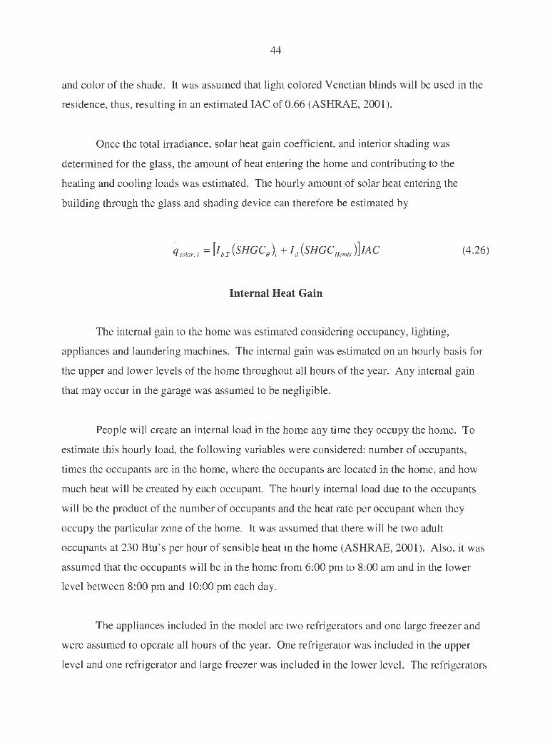
44
and color of the shade. It was assumed that light colored Venetian blinds will be used in the
residence, thus, resulting in an estimated IAC of 0.66 (ASHRAE, 2001).
Once the total irradiance, solar heat gain coefficient, and interior shading was
determined for the glass, the amount of heat entering the home and contributing to the
heating and cooling loads was estimated. The hourly amount of solar heat entering the
building through the glass and shading device can therefore be estimated by
Internal Heat Gain
(4.26)
The internal gain to the home was estimated considering occupancy, lighting,
appliances and laundering machines. The internal gain was estimated on an hourly basis for
the upper and lower levels of the home throughout all hours of the year. Any internal gain
that may occur in the garage was assumed to be negligible.
People will create an internal load in the home any time they occupy the home. To
estimate this hourly load, the following variables were considered: number of occupants,
times the occupants are in the home, where the occupants are located in the home, and how
much heat will be created by each occupant. The hourly internal load due to the occupants
will be the product of the number of occupants and the heat rate per occupant when they
occupy the particular zone of the home. It was assumed that there will be two adult
occupants at 230 Btu's per hour of sensible heat in the home (ASHRAE, 2001). Also, it was
assumed that the occupants will be in the home from 6:00 pm to 8:00 am and in the lower
level between 8:00 pm and 10:00 pm each day.
The appliances included in the model are two refrigerators and one large freezer and
were assumed to operate all hours of the year. One refrigerator was included in the upper
level and one refrigerator and large freezer was included in the lower level. The refrigerators

45
were assumed to emit 900 Btu's per hour each and the freezer was assumed to emit 2,760
Btu 's per hour (ASHRAE, 2001).
Also, the heat generated by doing laundry was considered. It was assumed that the
laundry machines will operate on each Saturday of the year for two hours, 9:00 am to 11 :00
am. The heat emitted into the home by the washer and dryer were estimated to be
approximately 4,100 Btu's per hour (ASHRAE, 2001).
Lastly, the home lighting was considered. Heat gained to the home from lights was
assumed to occur during times when the occupants are home and awake and also when there
is no solar gain. The number of lights used was assumed to be eight, each at one-hundred
watts. A summary of all inputs to the internal gain model can be seen in Table 4.4.
Table 4.4: Internal gain model inputs
HOMEOWNER PROFILE - INTERNAL GAINS Heat load per occupant (Btu/hr) 230 (SH) Number of occupants 2 Typical time occupants go to lower level of home 20 Typical time occupants return to upper level of home 22 Home occupied from (PM TIME) 18 Home occupied to (AM TIME) 8 Constant load from uooer level aooliances (Btu/hr) 900 Constant load from lower level aooliances (Btu/hr) 3660 Load from lights on uooer level when no solar (Btu/hr) 2,730 Load from liqhts on lower level when no solar (Btu/hr) 2,730 Load from clothes washer and dryer (Btu/hr) 4,094 Day laundry is done Sat Hour of launderinq 9 Hour' of launderinq 10 Typical time occupants qo to sleep 22 Typical time occupants awake from sleep 6 If solar qain is qreater than X Btuh then no liqhts 0
The hourly internal gain to the home was estimated by
q int ernal, i = q occupancy, i + q lights , i + q appliances, i + q laundry, i (4.27)

46
Monthly and Annual Heating Loads
The hourly heat losses from the home were estimated for the upper level, lower level,
and garage separately by
q heating ,i = [ q transmission ,i + q inf iltration,i - q solar,i - q int ernal,i ]+ (4.28)
where the + sign represents only positive hourly values were used in the monthly and annual
energy estimations. A negative value for an hourly heating load would represent a net heat
gain to the home for that hour and heating from the HV AC system would not need condition
the indoor air.
The total monthly heat loss of the home is then the sum of the hourly upper level,
lower level, and garage heat losses for each month. Similarly, the annual total heat loss of
the home is the sum of the hourly upper level, lower level, and garage heat losses over the
entire year.
Table 4.5: Monthly and annual estimated total home heat loss
Upper Level Lower Level Garage Ht. Total Home Ht. Loss Ht. Loss Loss Ht. Loss
Period (MMBtuh) (MMBtuh) (MMBtuh) (MMBtuh) January 16.19 11 .16 6.31 33.66 February 10.81 7.31 3.97 22.09 March 7.35 4.58 2.31 14.23 April 3.76 1.94 0.91 6.61 Mav 1.08 0.31 0.07 1.46 June 0.32 0.04 0.00 0.37 July 0.12 0.01 0.00 0.14 Auqust 0.30 0.03 0.00 0.34 September 1.09 0.30 0.08 1.48 October 3.53 1.77 0.70 6.00 November 7.29 4.45 1.99 13.73 December 12.50 8.17 4.32 25.00 Annual 64.35 40.08 20.67 125.11
Individual homeowners may turn on the heating system to their home at different
times; for example, homeowner x may turn on the heating system when it is 50°F outdoors,

47
and homeowner y may turn prefer to turn on the heat when it is 60°F outside. The hourly
heating load was set to zero if the outdoor temperature was above the particular outdoor air
temperature specified by the owners. Through conversations with the owners of the case
study home it was determined that the heating system would most likely not be turned on if
the outdoor air temperature was greater than 50°F. Table 4.6 shows the prorated energy uses
of the home with the minimum outdoor air temperature criteria.
Table 4.6: Monthly and annual estimated total home heat loss with outdoor air temperature constraint
Upper Level Lower Level Garage Ht. Total Home Ht. Loss Ht. Loss Loss Ht. Loss
Period (MMBtuh) (MMBtuh) (MMBtuh) (MMBtuh) January 16.19 11 .16 5.93 33.28 February 10.68 7.30 3.68 21.66 March 7.20 4.55 1.69 13.44 April 3.14 1.84 0.38 5.35 May 0.35 0.19 0.00 0.54 June 0.02 0.01 0.00 0.03 July 0.00 0.00 0.00 0.00 Auqust 0.00 0.00 0.00 0.00 September 0.49 0.21 0.00 0.70 October 3.02 1.68 0.15 4.86 November 7.10 4.41 1.28 12.79 December 12.50 8.17 3.84 24.51 Annual 60.68 39.52 16.94 117.14
It can be seen that by including the minimum outdoor air temperature constraint the annual
estimated heating load to the home on the HV AC system decreased by 6.37 percent.
Monthly and Annual Cooling Loads
The hourly heat gains to the upper and lower levels of the home were estimated by
[ ]+
. . . . .
q cooling ,; = q transmission,i + qinf iltration,i + q solar,i + q int emal,i (4.29)
where the + sign represents only positive hourly values were used in the monthly and annual
energy estimations. A negative value for hourly heat gain would represent a net heat loss

48
from the home for that hour conditioning the indoor air would be unnecessary. The hourly
heat gains were then summed up for each month and annually and are tabulated in Table 4.7.
Table 4.7: Monthly and annual estimated total home heat gain
Total Home Period Ht. Gain
(MMBtuh) January 0.24 February 0.30 March 1.57 April 3.19 May 5.61 June 8.93 July 12.51 Auqust 10.09 September 5.70 October 3.35 November 0.87 December 0.27 Annual 52.65
Table 4.7 represents the heat gain to the home with no ventilation. To more
accurately predict the amount of heat gain seen by the HV AC system, all heat gain values
that occur at or below a particular outdoor air temperature are assumed to be zero, and the
home will be assumed to be open to free ventilation. The owners expressed that they would
most likely turn on the air conditioning when the outdoor air temperature reached 80°F.
Table 4.8 shows the prorated energy uses of the home with the maximum outdoor air
temperature criteria.
It can be seen that by including the maximum outdoor air temperature constraint the
annual estimated cooling load to the home and supplied by the HV AC system decreased by
approximately a factor of three (285 percent).

49
Table 4.8: Monthly and annual estimated total home heat gain with outdoor air temperature constraint
Total Home Period Ht. Gain
(MMBtuh) Januarv 0.00 February 0.00 March 0.00 April 0.25 May 0.76 June 3.47 July 8.05 Auqust 5.54 September 1.38 October 0.40 November 0.00 December 0.00 Annual 19.86
Forced Air System Operating Performance and Costs in the Heating Mode
The hourly demand on the forced air distribution system and radiant floor system
must be determined separately so that the operating performance and costs of each can be
found. To estimate the amount of heating supplied by each system on an hourly basis, the
control scheme for each system must be determined. It was decided that the forced air
heating supplied by the heat pump or furnace will be controlled by one thermostat located on
the upper level. The radiant floor heating will be controlled by two thermostats, one on the
lower level and one in the garage. The forced air heating will turn on when the upper level
temperature drops below 68°F, and the radiant floor heating will turn on when the heating
supply from the forced air system to the lower level is insufficient to maintain 68°F and/or
when the garage temperature drops below 50°F.
To compromise between efficient heating with the heat pump and extra comfortable
heating with the radiant floor to the lower level, it was decided that the radiant floor heating
system would not be turned on until the outdoor air temperature has dropped to a low value.
The owners of the case study home were consulted, and they determined that they would like
the radiant floor heating in the lower level to turn on when the outdoor air temperature is near
or below 25 degrees Fahrenheit. As a result, the owners will be able to heat the lower level

50
efficiently with the heat pump most of the time, and enjoy the comfort of the radiant floor
heat when the heat loss of the lower level is high causing uneven space temperatures.
Knowing that the owners would like the radiant floor heating to turn on in the lower
level at about 25°F, the amount of energy required by the forced air system to the lower level
can be estimated. The average load of the lower level at the specified outdoor air
temperature was found by the ratio of the sum of each load for the lower level that
corresponded to an outdoor air temperature between 24.8°F and 25.2°F to the number of
times the outdoor air temperature fell within that range. Thus, the result is the amount of
heat that must be supplied to the lower level so that no radiant floor heating takes place; for
temperatures below this range, the radiant floor heating will be required.
Ground-Source Heat Pump
This section will describe the methods used to predict the hourly performance of the
ground-source heat pump and costs. This evaluation will begin with estimating the operating
characteristics of the heat pump as an ultimate function of the outdoor air temperature. Then,
considering the hourly loads on the home, the hourly performance of the heat pump used in
conjunction with the radiant floor will be estimated.
The capacity of the heat pump can be found if the following parameters are known:
the air flow rate through the coil, entering water temperature, compressor speed, whether or
not the heat pump is creating domestic hot water, and water flow rate. It was assumed that
the air and water flow rates through the unit in high speed are 14 gpm and 2,000 cfm; the low
speed conditions were assumed to be 11 gpm and 1,100 cfm. In addition, for this analysis it
was assumed that the heat pump will not be creating hot water.
To determine the heat pump capacity in both high and low speeds as a function of
entering water temperature, the manufacturer's specifications were used. The capacity
information from the specifications was plotted and lines were fit to obtain an equation

51
relating entering water temperature to heating capacity for the entire range of entering water
temperatures.
Heating Capacity of E060 WaterFurnace Heat Pump
100
90
80
:2 70 :::,
iii e 60 ~ ·u (II 50 C.
--+- High Spd. Heating Only
(II
u -.- Low Spd. Heating Only en 40 .!: iii 30 Q)
J:
20
10
0
0 20 40 60 80 100
EWT (F)
Note: 14 GPM and 2000 CFM for High Spd.; 11 GPM and 1100 CFM for Low Spd.
Figure 4. 7: Heating capacity of Water Furnace EO60 heat pump
The heating capacity of the heat pump in high speed was found to be
HC = -0.002l25(EWT)2 + l.119(EWT)+6.2225 (4.30)
with an R2 value of 0.999995.
The heating capacity of the heat pump in low speed was found to be
HC = -0.0008(EWT)2 +0.571(EWT)+ 1.4963 (4.31)
with an R2 value of 0.9995.

52
The hourly entering water temperature can be roughly estimated using methods
developed by the International Ground Source Heat Pump Association (IGSHPA). This
method relates the minimum, maximum and mean outdoor air temperature, undisturbed deep
ground temperature, and design entering water temperatures in the heating and cooling mode
and is stated for heating as
EWI .=DEWI +[EWIMEAN-DEWIM1N][oAT-oAT ] H,, MIN OAT -OAT l MIN
MEAN MIN (4.32)
and for cooling as
EWI . = EWI + [DEWIMAX - EWIMEAN] [OAT -OAT ] c,, MEAN OAT - OAT l MEAN
MAX MEAN (4.33)
where the EWT MEAN is equal to the undisturbed deep ground temperature or the average
annual outdoor air temperature plus two degrees Fahrenheit. A general plot of Equations
4.32 and 4.33 can be seen in Figure 4.8.
EWT
EWTMAX
SUMMER
EWTMEAN
WINTER EWTMIN
TA
OATMIN OAT MEAN OAT MAX
Figure 4.8: Plot of entering water temperature as a function of outdoor air temperature

53
It can be seen from Figure 4.8 that the entering water temperatures vary throughout the year
between the design temperatures, which were chosen to be 35 and 75 degrees Fahrenheit.
The estimated hourly entering water temperatures to the heat pump over the entire year were
plotted and can be seen in Figure 4.9.
Hourly Entering Water Temperatures to the Ground-Source Heat Pump
80
70
~ 60 I!! :::,
°E 50 Q) C. E Q)
': 40 .! 10 ~ Cl 30 C: ·.: .! in 20
10
0 0 1000 2000 3000 4000 5000 6000 7000 8000 9000
Hour of Year
Figure 4.9: Hourly entering water temperature to heat pump
The system can now be simulated over the entire year using the hourly loads to the
home determined in the prior sections. The heating supply from the forced air system to the
lower level was chosen to be approximately 12.5 MBtuh for the heat pump on high speed.
The volume flow rate of air to the lower level when the heat pump is on high speed can be
determined by
Q= q 1.1 (T LAT - T indoorair )
(4.34)
where the load is in Btu's per hour.

54
The average leaving air temperature of the heat pump in heating mode on high speed
was estimated to be approximately 92°F by examining the specifications of the heat pump at
entering water temperatures between 50°F and 30 °F and at 2000 CFM. As a result, the
volumetric flow rate of air to achieve 12.5 MBtu's per hour in the lower level was calculated
to be approximately 470 CFM. This flow rate can be achieved by closing the diffusers in the
basement until the total specified volume flow rate of air is obtained and can be measured by
a flow hood.
The capacity of the heat pump in low speed is approximately half of the high speed
capacity. Thus, the energy supplied to the lower level will also decrease by approximately
half since the positions of the diffusers will remain constant. Consequently, it was assumed
that 6.25 MBtu's per hour will be supplied to the lower level when the heat pump is on low
speed.
The speed of the heat pump for each hour of the year was determined by evaluating
the difference between the upper level load and heat pump capacity available to the upper
level in both speeds. When the low speed capacity minus 6.25 MBtu ' s per hour was larger
than the upper level load, the unit was assumed to be in low speed, otherwise, the heat pump
was assumed to be operating in high speed. With the hourly speed and capacity of the heat
pump known, the hourly theoretical run time fraction of the heat pump could be determined
by
. . . Upper Level Demand . Theoretical Run T1me Fractwn = ' ( 4.35)
' Heat Pump Capacity ; - Lower Level Supply;
If the upper level load was greater than the heat pump capacity minus the lower level supply
for the particular hour, the theoretical run time was set to equal unity, i.e., the heat pump will
run the entire hour.

55
To estimate the actual run time of the heat pump for the hour, the partial load factor
(PLF) was determined. The PLF is an adjustment factor that accounts for the loss in
efficiency of the unit due to on-off cycling, which can be compensated for by increasing the
run time. The hourly PLF was determined by
PLF = 1 _ C [l -_____ U....:.p...:..p_e_r_L_e_v_el_D_e_m_a_n_d-'--i ----] ' D Heat Pump Capacityi - Lower Level Supplyi
(4.36)
The actual run time is the ratio of the theoretical run time to the partial load factor and is
stated as
l T . TheoreticalRun Timei Actua Run 1mei = -------
Partial Load Factor; (4.37)
The hourly heating supply of the heat pump for the upper and lower levels was determined
by
Heat Pump Supplyi = Upper Level Demand;
+(Theo.Run Fractioni )* Lower Level Supply; (4.38)
If the heat pump capacity on high speed for a particular hour minus the lower level
supply for that hour is less than the upper level demand, the heat pump will meet the demand
by using the electric resistance auxiliary heat. The amount of electric resistance auxiliary
heat in kWh that will be required of the heat pump for each hour can be determined by
Upper Lev. Dmnd; - (Heat Pump. Cap. ; - Lower Lev. Supply ;) Ele. Resis. Au.x,i = ---------------------- (4.39)
3.412
where the upper level demand, heat pump capacity, and lower level supply are in MBtu ' s per
hour.

56
The total electrical input to the heat pump can be found by
Heat Pump Tot. Ele. Input; = Actual Run Fract. ; * (Unit /nput ;+Ele. Resis. Aux.i) (4.40)
The electrical input of the heat pump in heating mode was determined in a similar
manner as for the capacity and can be seen in Figure 4.10.
5
4.5
4
3.5
[ 3
Heating Mode Power Draw of E060 WaterFurnace Heat Pump
_____. ~
~
:t ~ 2.5
ai
• High Spd. Heating Only
A Low Spd. Heating Only
~ 2 Q.
1.5
0.5
0
.
0 10 20 30 40
-
50
EWT (F)
__... . --
60 70 80 90 100
Note: 14 GPM and 2000 CFM for High Spd.; 11 GPM and 1100 CFM for Low Spd.
Figure 4.10: Power draw of heat pump in heating mode
The power draw of the heat pump in the heating mode on high speed was found to be
PD= -0.0000l2(EWT)2 +0.024700(EWT)+ 2.60925
with an R2 value of 0.9978.
The power draw of the heat pump in the heating mode on low speed was found to be
(4.41)

57
PD = 0.000006 (EWT )2 + 0.0049 (EWT) + 1.402875 (4.42)
with an R2 value of 0.9937.
Since the heat pump is controlled by only one thermostat, there may be times where
the lower level is being supplied too much air. This energy was determined as the difference
of the total supply and the total home demand and can be seen in Table 4.9. A summary of
the estimated monthly and annual heating supply of the forced air system, radiant floor
system, and both can be seen in Table 4.9.
Table 4.9: Monthly and annual heating supply of HV AC system using ground-source heat pump for forced air distribution system
Time Air Side Upper Water Side Water Side Lower Total Air and Total Extra
Period and Lower Level Garage Supply Lev. Supply Water Supply Heat to LL Supply (MMBtuh) (MMBtuh) (MMBtuh) (MMBtuh) (MMBtuh)
January 21.42 5.93 6.02 33.37 0.092 February 14.18 3.68 3.87 21.72 0.070 March 9.39 1.69 2.43 13.50 0.067 April 4.06 0.38 0.96 5.40 0.051 May 0.45 0 0.09 0.54 0.002 June 0.03 0 0 0.03 0 July 0 0 0 0 0 Auqust 0 0 0 0 0 September 0.63 0 0.08 0.70 0.003 October 3.91 0.15 0.84 4.90 0.048 November 9.23 1.28 2.34 12.86 0.068 December 16.52 3.84 4.21 24.57 0.059 Annual 79.82 16.94 20.84 117.60 0.461
Using an electric rate of $0.035 dollars per kWh for heating, the hourly operating
costs were determined by
Heating Cost; = [(Actual Run Time Fraction); * PD;+ Aux. HeatJ* Electric Rate (4.43)
A summary of the monthly and annual heating costs of the heat pump can be seen in Table
4.10.

58
Table 4.10: Monthly and annual heating costs of ground-source heat pump
Time Total Heat
Period Pump Cost
($) January $62 February $37 March $23 April $10 May $1 June $0 July $0 Auqust $0 September $2 October $9 November $22 December $42 Annual $208
Gas-Fired Furnace
It was determined that 12.5 MBtuh will be supplied to the lower level by the forced
air system in order to restrict the use of the radiant floor heating. Often the furnaces used for
residential applications are single speed (i.e., on or off). Thus, the heating supply to the
lower level by the furnace would be approximately 12.5 MBtuh whenever the upper level
calls for heating. Again, Equation 4.34 was used to determine the volumetric flow rate of air
to the lower level to achieve 12.5 MBtuh. The leaving air temperature of the furnace was
assumed to be 105°F, resulting in approximately 310 cubic feet per minute of air.
The capacity of the furnace that was recommended by the contractor is 120 MBtu's
per hour as seen in the quotation in Appendix D. When the furnace is operating it will
supply 108 MBtu's per hour to the upper level after accounting for the unit's efficiency. The
theoretical run time fraction of the furnace was determined using Equation 4.35. The hourly
heating supply of the furnace for the upper and lower levels was determined by
Furnace Supply;= Upper Level Demand;
+ (Theo. Run Fraction;)* Lower Level Supply; (4.44)

59
The hourly heating demand of the radiant floor system for the lower level was
determined. The hourly heating demand of the radiant floor system for the garage is equal to
the hourly heat loss in the garage.
A summary of the estimated monthly and annual heating supply of the furnace and
radiant floor and both can be seen in Table 4.11.
Table 4.11: Monthly and annual heating supply of HV AC system using liquid propane furnace for the forced air distribution system
Time Air Side Water Side Water Side Lower Total Air and Total Extra
Period Demand Garage Demand Lev. Demand Water Demand Heat to LL
(MMBtuh) (MMBtuh) (MMBtuh) (MMBtuh) (MMBtuh) January 17.88 5.93 9.49 33.29 0.0114 February 11.79 3.68 6.20 21 .67 0.0123 March 7.95 1.69 3.82 13.45 0.0140 April 3.46 0.38 1.52 5.36 0.0116 May 0.39 0.00 0.15 0.54 0.0004 June 0.02 0.00 0.01 0.03 0.0000 Julv 0.00 0.00 0.00 0.00 0.0000 August 0.00 0.00 0.00 0.00 0.0000 September 0.54 0.00 0.16 0.70 0.0010 October 3.34 0.15 1.37 4.87 0.0128 November 7.83 1.28 3.69 12.80 0.0124 December 13.80 3.84 6.88 24.51 0.0067 Annual 67.00 16.94 33.28 117.22 0.0826
To estimate the monthly and annual cost of operating a gas-fired furnace, the
efficiency of the unit was assumed to be constant. Thus, the cost per unit energy can be
determined for the furnace by
( $ )( Gallon J( 1,000,000 Btu J( 1 ) $ Gallon 91,600Btu MMBtuHeating A.F.U.E. MMBtuHeating
(4.45)
The manufacturer of the furnace states that the A.F.U.E. of the unit is 92 percent. Using the
monthly and annual energy demand and cost per unit energy, the monthly and annual costs
were estimated.
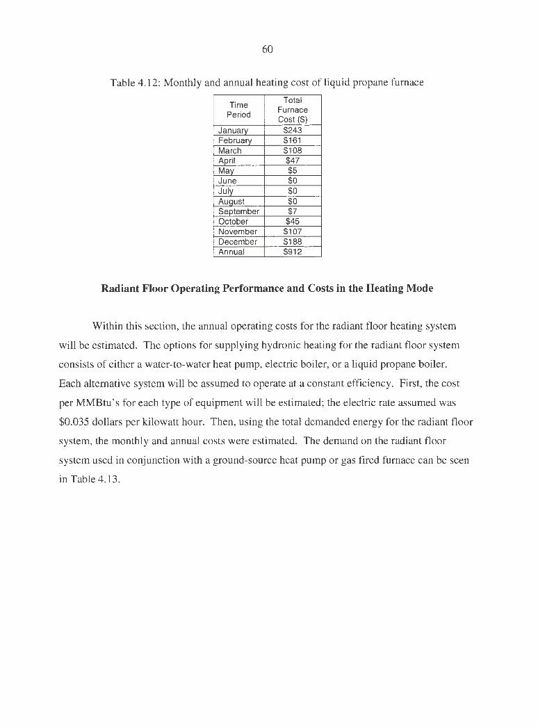
60
Table 4.12: Monthly and annual heating cost of liquid propane furnace
Time Total Furnace
Period Cost($)
Januarv $243 February $161 March $108 Aoril $47 May $5 June $0 July $0 Auoust $0 September $7 October $45 November $107 December $188 Annual $912
Radiant Floor Operating Performance and Costs in the Heating Mode
Within this section, the annual operating costs for the radiant floor heating system
will be estimated. The options for supplying hydronic heating for the radiant floor system
consists of either a water-to-water heat pump, electric boiler, or a liquid propane boiler.
Each alternative system will be assumed to operate at a constant efficiency. First, the cost
per MMBtu' s for each type of equipment will be estimated; the electric rate assumed was
$0.035 dollars per kilowatt hour. Then, using the total demanded energy for the radiant floor
system, the monthly and annual costs were estimated. The demand on the radiant floor
system used in conjunction with a ground-source heat pump or gas fired furnace can be seen
in Table 4.13.

61
Table 4.13: Monthly and annual demand on radiant floor system using either a ground-source heat pump or liquid propane furnace for the forced air distribution system
Water Side Water Side Lower Lev. Time Garage Demand (MMBtu)
Period Demand GSHP
Gas Fired (MMBtu) Furnace
January 5.93 6.02 9.49 February 3.68 3.87 6.20 March 1.69 2.43 3.82 April 0.38 0.96 1.52 May 0.00 0.09 0.15 June 0.00 0.00 0.01 July 0.00 0.00 0.00 August 0.00 0.00 0.00 September 0.00 0.08 0.16 October 0.15 0.84 1.37 November 1.28 2.34 3.69 December 3.84 4.21 6.88 Annual 16.94 20.84 33.28
The cost per MMBtu's for the heat pump and electric boiler were determined by
( $ )( kW )( W h )[l,000,000BtuJ( 1 ) $ kWh lOOOW 3.412 Btu MMBtuHeating COP = MMBtuHeating
(4.46)
The COP of the water-to-water heat pump and electric boiler was assumed to be a
constant value of 3.8 and 0.95, respectively. As a result, the costs per MMBtu's using the
heat pump and electric boiler were found to be $2.70 and $10.80 dollars, respectively. The
cost per MMBtu's using the liquid propane boiler was determined to be $13.53 dollars using
Equation 4.46 and assuming $1.14 dollars per gallon.
The estimated monthly and annual heating costs for each system were calculated by
[ $ J(MMBtuHeating ) $Heating MMBtuHeating Period - Period
(4.47)
where period represents the time period of either a month or year.

62
The estimated cost of using an electric boiler for the radiant floor heating with either
the heat pump or furnace can be seen in Table 4.14.
Table 4.14: Monthly and annual cost for electric boiler using either a ground-source heat pump or liquid propane furnace for the forced air distribution system
Time Total Electric Boiler Cost ($)
Gas Fired Period GSHP Furnace
January $129 $165 February $82 $106 March $44 $59 April $14 $20 May $1 $2 June $0 $0 July $0 $0 AUQUSt $0 $0 September $1 $2 October $11 $16 November $39 $53 December $87 $115 Annual $408 $538
The estimated cost of using a water-to-water heat pump for the radiant floor heating
with either the heat pump or furnace can be seen in Table 4.15.
Table 4.15: Monthly and annual cost for water-to-water heat pump using either a groundsource heat pump or liquid propane furnace for the forced air distribution system
Total Water-to-Water Time Heat Pump Cost ($)
Period GSHP
Gas Fired Furnace
January $32 $41 February $20 $26 March $11 $15 April $4 $5 May $0 $0 June $0 $0 July $0 $0 AUQUSt $0 $0 September $0 $0 October $3 $4 November $10 $13 December $22 $29 Annual $102 $134

63
The estimated cost of using a liquid propane boiler for the radiant floor heating with
either the heat pump or furnace can be seen in Table 4.16.
Table 4.16: Monthly and annual cost for liquid propane boiler using either a ground-source heat pump or liquid propane furnace for the forced air distribution system
Time Total L.P. Boiler Cost($)
Gas Fired Period GSHP Furnace
January $162 $207 February $102 $133 March $56 $74 April $18 $25 Mav $1 $2 June $0 $0 July $0 $0 Auqust $0 $0 September $1 $2 October $13 $20 November $49 $66 December $109 $144 Annual $511 $673
Forced Air System Operating Performance and Costs in the Cooling Mode
Ground-Source Heat Pump
The method used in determining heat pump performance in the cooling mode was
performed in a similar manner as with the heating load. First, the capacity of the heat pump
in cooling mode was plotted and equations were obtained for the cooling capacity as a
function of entering water temperatures.
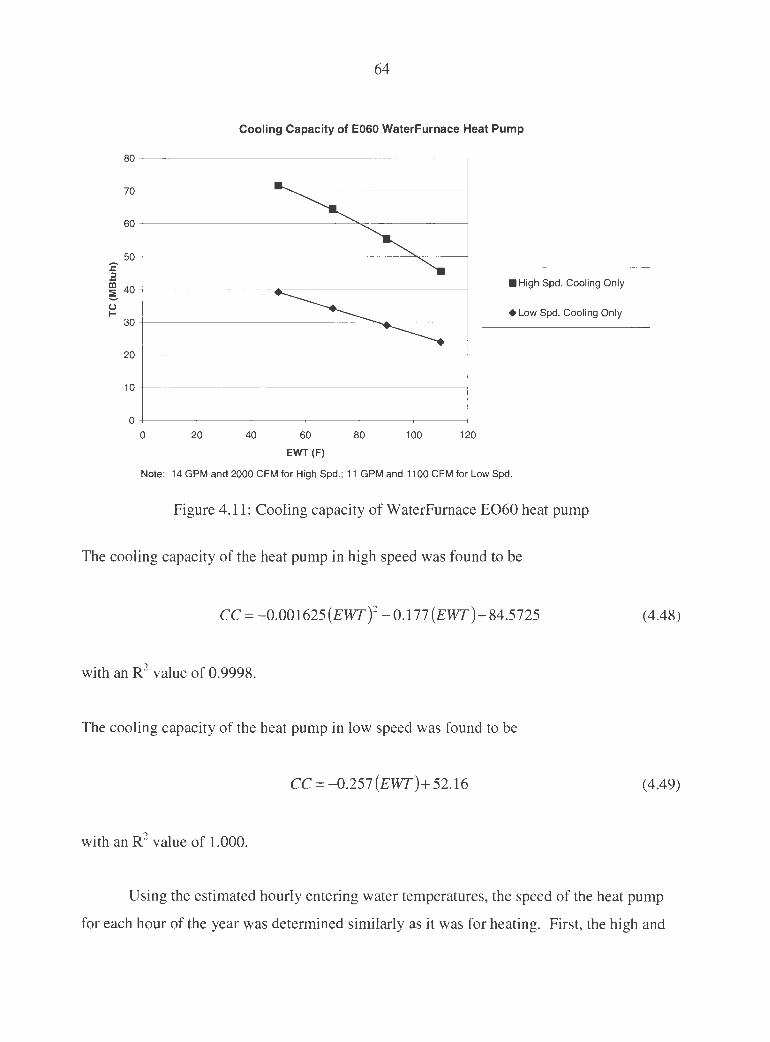
64
Cooling Capacity of E060 WaterFurnace Heat Pump
80
70
60
50 :2 :I
ai 40 e • High Spd. Cooling Only
0 I- • Low Spd. Cooling Only
30
20
10
0
0 20 40 60 80 100 120
EWT (F)
Note: 14 GPM and 2000 CFM for High Spd.; 11 GPM and 1100 CFM for Low Spd.
Figure 4.11: Cooling capacity of WaterFumace EO60 heat pump
The cooling capacity of the heat pump in high speed was found to be
CC= -0.001625(EWT)2 -0.177(EWT)+84.5725 (4.48)
with an R2 value of 0.9998.
The cooling capacity of the heat pump in low speed was found to be
CC =-0.257(EWT)+52.16 (4.49)
with an R2 value of 1.000.
Using the estimated hourly entering water temperatures, the speed of the heat pump
for each hour of the year was determined similarly as it was for heating. First, the high and

65
low speed capacities were calculated for each hour using the fitted equations with respect to
the corresponding entering water temperature. Next, the capacities were compared to the
total hourly load. It was assumed that the lower level will be supplied the correct amount of
cooling; as a result, the control for the heat pump was not determined by the upper level load
alone. If the capacity of the heat pump in low speed was sufficient to meet the total load,
then the unit was assumed to be operating in low speed for that hour; otherwise, the unit was
assumed to be in high speed.
The hourly theoretical run time fraction of the heat pump is the ratio of the total home
cooling load to the heat pump capacity at each respective hour.
. . . Total Home Demand . Theoretical Run Time Fractwn; = '
Heat Pump Capacity; (4.50)
If the heat pump capacity was determined to be less than the load, then the theoretical run
time fraction was assumed to be unity, i.e., the heat pump is assumed to run for the entire
hour. The hourly part load factor that considers loss of efficiency due to cycling was
determined by
PLF = l-C [l- Total Home Demand; ] ' D Heat Pump Capacity;
(4.51)
The actual run time fraction was then determined by equation 4.37.
The power draw of the heat pump was determined as a function of the entering water
temperature as before from the manufacturer's specifications, seen in Figure 4.12.

66
Cooling Mode Power Draw of E060 WaterFurnace Heat Pump
3.5 +-------- ---------7""~-------------j
[ 3 +--- - - ----~ -----------------1~----- -~
:!: g 2.5 +----- ------ - --- --- - - - - --------1 • High Spd. Cooling Only
lii A Low Spd. Cooling Only ~ 2 -t--------- ------ - -------=;;------,~-- --- -~ C.
0 +--------- - - ~--- ~---~-------1
0 20 40 60
EWT (F)
80 100
Note: 14 GPM and 2000 CFM for High Spd.; 11 GPM and 1100 CFM for Low Spd.
120
Figure 4.12: Power draw of heat pump in cooling mode
The power draw of the heat pump in the cooling mode on high speed was found to be
PD= 0.02795 (EWT)+ 1.6765
with an R2 value of 0.9979.
The power draw of the heat pump in the cooling mode on low speed was found to be
PD= 0.01555(EWT)+ 0.3135
with an R2 value of 0.9986.
(4.52)
(4.53)
Finally, using an electric rate of $0.091 dollars per kWh for cooling, the operating
costs were estimated by

67
Cooling Cost; = PD; * (Actual Run Time Fraction); * Electric Rate (4.54)
A summary of the monthly and annual cooling costs using the heat pump can be seen in
Table 4.17.
Table 4.17: Monthly and annual cooling cost of ground-source heat pump
Total Cooling Period Cost
($) January $0 February $0 March $0 April $2 May $4 June $21 July $56 Auqust $35 September $8 October $2 November $0 December $0 Annual $128
Air Conditioner
Assuming that the efficiency of the typical air conditioner is constant, the cost per
unit energy for cooling was determined by
( $ )( kW J(l,000,000BtuJ(w h) $ kWh 1000 W MMBtucooling Btu = MMBtucooling
(4.55)
The last product in units of watt-hours per Btu (Wh/Btu) is the reciprocal of the air
conditioner' s EER and will be assumed to be 12, which is typical. Using an electric cost in
the summer of $0.091 dollars per kilowatt hour the cost per MMBtu ' s was found to be $7.58
dollars.
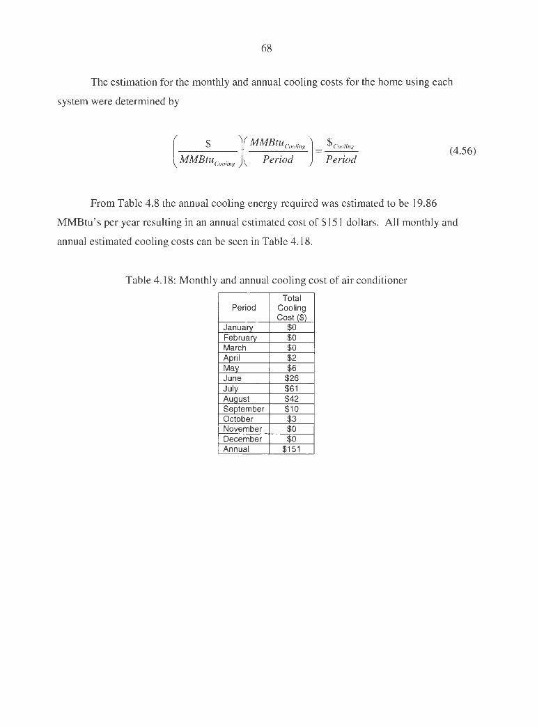
68
The estimation for the monthly and annual cooling costs for the home using each
system were determined by
[ $ J(MMBtuCooling J $Cooling
MMBtucooling Period - Period (4.56)
From Table 4.8 the annual cooling energy required was estimated to be 19.86
MMBtu's per year resulting in an annual estimated cost of $151 dollars. All monthly and
annual estimated cooling costs can be seen in Table 4.18.
Table 4.18: Monthly and annual cooling cost of air conditioner
Total Period Cooling
Cost($) January $0 February $0 March $0 April $2 May $6 June $26 July $61 August $42 September $10 October $3 November $0 December $0 Annual $151

69
CHAPTER 5 - ECONOMICS OF ALTERNATIVE APPROACHES
In this section, each of the three main alternative approaches will be compared
economically using a life-cycle-cost analysis. First, all of the annual expenses for each
approach were predicted over the life of the system. Then, the annual savings for each
approach was determined in comparison to the conventional system. Finally, the present
value for each approach was determined assuming an estimated interest rate on an alternative
investment. Once this analysis was completed, the present values for each of the three
alternative approaches were compared, which revealed the most economical system for the
owners.
Expenses
The expenses for each heating and cooling approach will comprise the following:
annual operation costs, equipment and installation costs, and interest payments on a loan.
The maintenance costs for each approach were assumed to be the same for all systems and
were not considered in the analysis. Each expense will initially be analyzed individually on
an annual basis. Then, each annual expense will be summed together to obtain the total
annual cost for implementing each approach.
The three main factors that most significantly contribute to the annual cost of
operation for each approach are: the cost per unit of energy, volatility of future energy cost,
and the overall system efficiency. Examining the alternative approaches, the residence will
be dependant upon electricity for their heating and cooling needs in some way or another.
The cost for electricity will vary depending on which utility is used, the benefits offered by
that utility, the season, and the geographical location of the home. The utility that will be
used at the residence is MidAmerican, which offers stable rates including an all-electric
heating rate. The all-electric heating rate is a reduced electric rate that can be obtained in the
heating season if the home is dominantly heated with an electrical driven device, such as a
heat pump or electrical resistance heater.

70
The three alternative approaches will all be expected to utilize the all-electric heating
rate, where approach 4 will not due to the dominant heating source being liquid propane gas.
In addition, this reduced rate of electricity only applies to energy used in excess of 1,000
kilowatt hours (i.e. the first 1,000 kilowatt hours cost the regular rate and energy used in
addition to 1,000 kilowatt hours costs the all-electric heating rate). The reasoning for
offering this benefit after the first 1,000 kilowatt hours is based on the assumption that the
home will use this amount of energy for everyday uses (lights, appliances, etc.) and the
remainder is assumed to be used for heating the home. This is a benefit offered by the utility
to promote the use of electricity for means of heating opposed to an alternative source of
energy. The regular residence rate currently offered by the local utility is $0.091 dollars per
kilowatt hour. The all electric heating rate is currently $0.035 dollars per kilowatt hour after
all additional fees are applied.
To estimate the future increase in electricity rates, predictions formulated by the
National Institute of Standards and Technology (NIST) were used (Schultz, 2004). The
values in Table 5.1 represent the multiplier used to estimate the cost of electric for the
residential market for 25 years in the future at various general price inflation rates. The
utility that will be supplying electricity to the case study home has set a freeze on the cost of
electricity until the year 2010. As a result, the price of electricity at the residence is
guaranteed not to change for at least five years. Consequently, the price of electric until 2010
is known to be $0.091 dollars per kilowatt hour at the regular rate and $0.035 dollars per
kilowatt hour at the all electric rate. The electric price indices were adjusted to account for
the price freeze.

71
Table 5 .1: Projected electric price indices
Electricity Year Year General Price Inflation Rate (%)
2% 3% 4% 5% 0 2004 1 1 1 1 1 2005 1 1 1 1 2 2006 1 1 1 1 3 2007 1 1 1 1 4 2008 1 1 1 1 5 2009 1 1 1 1 6 2010 1.07 1.14 1.21 1.28 7 2011 1.09 1.17 1.25 1.34 8 2012 1.12 1.21 1.31 1.42 9 2013 1.16 1.26 1.38 1.5 10 2014 1.19 1.31 1.44 1.59 11 2015 1.22 1.35 1.51 1.67 12 2016 1.25 1.4 1.57 1.76 13 2017 1.27 1.44 1.64 1.85 14 2018 1.3 1.49 1.7 1.95 15 2019 1.32 1.53 1.76 2.04 16 2020 1.35 1.57 1.84 2.14 17 2021 1.38 1.63 1.92 2.26 18 2022 1.41 1.68 2 2.37 19 2023 1.43 1.72 2.07 2.48 20 2024 1.47 1.78 2.17 2.62 21 2025 1.5 1.84 2.26 2.76 22 2026 1.53 1.9 2.35 2.9 23 2027 1.57 1.96 2.45 3.05 24 2028 1.6 2.02 2.55 3.2 25 2029 1.63 2.08 2.65 3.37
Source: NIST, 2004
The cost of liquid propane gas is fairly unregulated and is currently volatile. The
current price of liquid propane gas for the heating season is approximately $1.14 dollars per
gallon. Again, to estimate the future cost of liquid propane gas, predictions from NIST were
used.

72
Table 5.2: Projected liquid propane price indices
L.P. Gas Year Year General Price Inflation Rate(%)
2% 3% 4% 5% 0 2004 1 1 1 1 1 2005 0.89 0.89 0.9 0.91 2 2006 0.87 0.88 0.9 0.92 3 2007 0.89 0.92 0.94 0.97 4 2008 0.92 0.95 0.99 1.03 5 2009 0.94 0.99 1.04 1.09 6 2010 0.96 1.02 1.08 1.15 7 2011 1 1.07 1.14 1.22 8 2012 1.02 1.11 1.2 1.29 9 2013 1.05 1.15 1.25 1.37 10 2014 1.08 1.19 1.31 1.44 11 2015 1.11 1.24 1.38 1.53 12 2016 1.15 1.29 1.45 1.62 13 2017 1.18 1.34 1.52 1.72 14 2018 1.21 1.38 1.58 1.81 15 2019 1.24 1.43 1.66 1.91 16 2020 1.27 1.48 1.73 2.02 17 2021 1.3 1.54 1.81 2.13 18 2022 1.33 1.59 1.89 2.25 19 2023 1.37 1.64 1.97 2.37 20 2024 1.4 1.7 2.06 2.5 21 2025 1.44 1.76 2.16 2.64 22 2026 1.47 1.82 2.25 2.78 23 2027 1.5 1.88 2.35 2.93 24 2028 1.54 1.94 2.45 3.08 25 2029 1.57 2.01 2.55 3.24
Source: NIST, 2004
The use of liquid propane gas at a residence has several other disadvantages in
addition to volatile rates. This fuel is not available for remote supply via gas lines to the
home from a utility. Therefore, the consumer will be required to maintain sufficient levels of
this fuel on-site year-round in a rented or purchased tank. Further, the consumer will benefit
if they commit to the gas price in the summer season by accepting to enter into a contract
with the supplier; thus, the consumer must monitor the current rate of the fuel in order to
obtain the best price throughout the year.
For this study, a long-term average inflation rate of three percent was assumed.
Using the corresponding price indices and annual operating cost estimated at current energy
costs, the future annual operation costs were found.

73
Table 5.3: Future annual operating costs using heat pump for forced air distribution system
Forced Air Radiant Floor
Year E060 Heat E060 Heat EW040 Electric Liquid Pump Pump Heat Boiler Propane
Heating Coolina Pump Boiler 2004 $208 $128 $102 $408 $511 2005 $208 $128 $102 $408 $455 2006 $208 $128 $102 $408 $450 2007 $208 $128 $102 $408 $470 2008 $208 $128 $102 $408 $486 2009 $208 $128 $102 $408 $506 2010 $237 $145 $116 $465 $521 2011 $244 $149 $119 $477 $547 2012 $252 $154 $123 $494 $567 2013 $262 $161 $129 $514 $588 2014 $273 $167 $134 $534 $608 2015 $281 $172 $138 $551 $634 2016 $291 $179 $143 $571 $659 2017 $300 $184 $147 $588 $685 2018 $310 $190 $152 $608 $705 2019 $319 $195 $156 $624 $731 2020 $327 $200 $160 $641 $756 2021 $339 $208 $166 $665 $787 2022 $350 $214 $171 $685 $813 2023 $358 $219 $175 $702 $838 2024 $371 $227 $182 $726 $869 2025 $383 $235 $188 $751 $900 2026 $396 $242 $194 $775 $930 2027 $408 $250 $200 $800 $961 2028 $421 $258 $206 $824 $992 2029 $433 $265 $212 $849 $1,027
The annual operating costs were also estimated for the conventional system and can
be seen in Table 5.4.
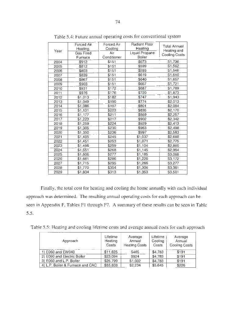
74
Table 5.4: Future annual operating costs for conventional system
Forced Air Forced Air Radiant Floor Total Annual
Year Heatinq. Cooling Heatinq
Heating and Gas Fired Air Liquid Propane Furnace Conditioner Boiler
Cooling Costs
2004 $912 $151 $673 $1,736 2005 $812 $151 $599 $1,562 2006 $803 $151 $593 $1,546 2007 $839 $151 $619 $1,610 2008 $867 $151 $640 $1 ,657 2009 $903 $151 $667 $1 ,721 2010 $931 $172 $687 $1 ,789 2011 $976 $176 $720 $1,873 2012 $1,013 $182 $747 $1 ,943 2013 $1,049 $190 $774 $2,013 2014 $1,086 $197 $801 $2,084 2015 $1 ,131 $203 $835 $2,170 2016 $1,177 $211 $869 $2,257 2017 $1,223 $217 $902 $2,342 2018 $1,259 $224 $929 $2,413 2019 $1 ,305 $230 $963 $2,498 2020 $1,350 $236 $997 $2,583 2021 $1,405 $245 $1 ,037 $2,688 2022 $1,451 $253 $1 ,071 $2,775 2023 $1 ,496 $259 $1 ,104 $2,860 2024 $1 ,551 $268 $1,145 $2,964 2025 $1,606 $277 $1,185 $3,068 2026 $1 ,661 $286 $1,226 $3,172 2027 $1 ,715 $295 $1 ,266 $3,277 2028 $1,770 $304 $1,306 $3,381 2029 $1 ,834 $313 $1 ,353 $3,501
Finally, the total cost for heating and cooling the home annually with each individual
approach was determined. The resulting annual operating costs for each approach can be
seen in Appendix F, Tables Fl through F7. A summary of these results can be seen in Table
5.5.
Table 5.5: Heating and cooling lifetime costs and average annual costs for each approach
Lifetime Average Lifetime Average Approach Heating Annual Cooling Annual
Costs Heating Costs Costs Cooling Costs
1) E060 and EW040 $11 ,625 $465 $4,783 $191 2) E060 and Electric Boiler $23,094 $924 $4,783 $191 3) E060 and L.P. Boiler $25,799 $1 ,032 $4,783 $191 4) L.P. Boiler & Furnace and CAC $55,838 $2,234 $5,645 $226

75
The initial equipment and installation costs for the same project can vary depending
on the contractor. Therefore, obtaining competitive bids for the project may be beneficial to
the consumer. Residentially, most contractors submit a "lump-sum" quote to the consumer
that does not break down costs for each individual item. As a result, determining cost
differences between alternative systems can become difficult. For the study, bids were
obtained for each alternative approach. It should be noted that approach 1 (i.e., all
geothermal) was initially bid using a nominal 6 ton water-to-water heat pump instead of a
nominal 2 ton heat pump. The bid price seen in Table 5.6 is a different estimated bid price
for replacing this unit.
Table 5.6: Initial cost for the equipment and installation of each alternative
Aooroach Svstem Bid Price 1 E060 and EW040 $50,000 2 E060 and Electric Boiler $35,900 3 E060 and L.P. Gas Boiler $37,000 4 L.P. Gas Furnace and Boiler and CAC $23,700
The annual interest costs on the loan can make a significant impact on the total cost of
the project. The residence under consideration will be purchased with an amortized loan
from a bank or other financial source for a term of 10 years. An amortized loan is a loan in
which the amount of interest owed for a specified period is calculated based on the remaining
balance of the loan at the beginning of the period (Park, 2002). The amount paid per period
on the loan is a constant amount, thus, the amount of interest paid and amount on the
principal paid will vary with each payment.
Initially, the amount of money to be paid per year on the loan was determined. The
size of payment is equal to the net present value (cost) of the system separated into annual
installments at the particular interest rate over the specified period of time. The average
percentage rate (APR) of the loan will be assumed to be 5.6 percent. The amount of each
annual installment can be calculated by

76
(5.1)
The amount of interest paid on the first payment can be found using
(5.2)
Knowing that the annual payment is equal to the interest amount plus the principal amount of
the payment, the amount of money paid on the principal for the first payment was found by
Pr1 = a - Ir,1
The remainder of the balance can be determined at the end of the first year after the first
payment using Equation 5.4.
(5.3)
(5.4)
Once the first values have been found, the remaining values for the term of the loan can be
found using Equations 5.5, 5.6, and 5.7.
(5.5)
(5.6)
Prn = a - I P.n (5 .7)
The annual interest paid, annual principal paid, and loan balance for each year for each
approach can be seen in Appendix E in Tables El through E4. A summary of the total loan
payments for the term of the loan can be seen in Table 5.7.

77
Table 5.7: Summary of loan payments and project costs of each approach
Total Total Total Cost
Difference from Approach Payments Interest
Conventional to Bank Paid System
1 $66,652 $16,652 $35,059 2 $47,856 $11,956 $16,263 3 $49,323 $12,323 $17,730 4 $31,593 $7,893 $0
Savings
The estimated savings for the three main approaches were considered by separating
the savings compared to the conventional system into several different categories, namely,
available rebates for installing a geothermal system, tax savings or "tax write-offs," and
operation savings.
The rebates that are available for installing a geothermal system are based on the
installed heating capacity of the system at the rate of $300.00 dollars per ton. This rebate is
given to the owner upon initial installation.
Table 5.8: Available rebate for each approach
Approach Installed Heating Available Capacity (Tons) Rebate($)
E060 and EW040 8 $2,400 E060 and Electric Boiler 5 $1,500 E060 and L.P. Boiler 5 $1,500 L.P. Boiler & Furnace and CAC 0 $0
The tax savings or "tax write-offs" will also contribute to the overall savings of the
project. The amount of tax savings to the consumer will be dependant on the tax bracket of
the consumer and the APR of the loan. The amount of interest paid on the loan will be tax
deductible. The consumer is in the 45 percent tax bracket; as a result, 45 percent of the
interest paid on the loan at a particular year will be saved in taxes. The amount of annual tax
savings for each approach can be determined by
Tax Savingsn = Tax Rate * (I P,J (5.8)

78
The total tax savings for the project is the summation of the annual tax savings over the life
of the loan.
10
Total Tax Savings= "'f.TaxSavingsn (5.9) n=l
The annual tax savings for each approach was determined and compared to the conventional
system. The annual tax savings for each approach can be seen in Appendix G Tables G 1
through 04. Seen in Table 5.9 is a summary of the results.
Table 5.9: Summary of tax savings for each approach
Total Tax Total Tax Savings Approach Savings Compared to
($) Conventional ($)
1 $7,494 $3,942 2 $5,380 $1 ,828 3 $5,545 $1,993 4 $3,552 $0
Finally, the annual and total operation savings was determined. The operating costs
for each approach are seen in Appendix F and in Table F.1. The savings for each of the three
approaches is the difference in operating costs between each approach and the conventional
approach. A summary of the total operation savings for each approach over the assumed
lifetime of the systems is shown in Table 5 .10.
Table 5. l 0: Summary of total operation savings for each approach
Lifetime Heating Lifetime Cooling Lifetime Total Approach Savings to Savings to Savings to
Aooroach 4 Approach 4 Aooroach 4 1 $44,212 $862 $45,074 2 $32,744 $862 $33,606 3 $30,038 $862 $30,900 4 $0 $0 $0
The annual operation savings for each approach can be seen in Appendix H.
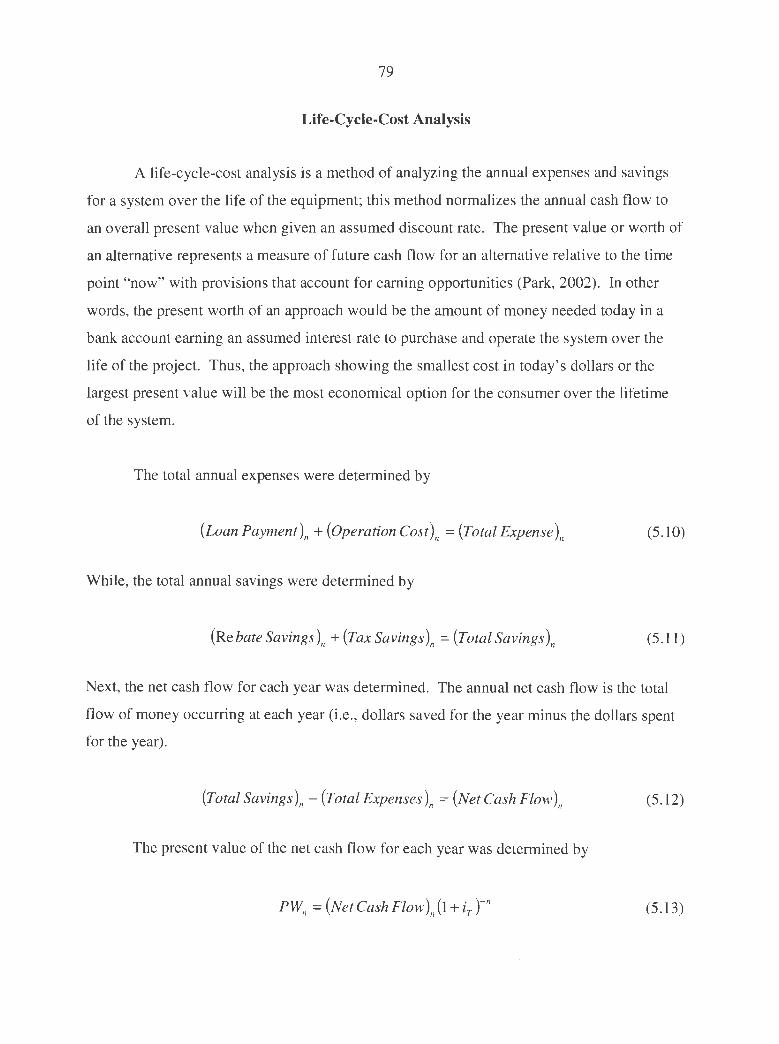
79
Life-Cycle-Cost Analysis
A life-cycle-cost analysis is a method of analyzing the annual expenses and savings
for a system over the life of the equipment; this method normalizes the annual cash flow to
an overall present value when given an assumed discount rate. The present value or worth of
an alternative represents a measure of future cash flow for an alternative relative to the time
point "now" with provisions that account for earning opportunities (Park, 2002). In other
words, the present worth of an approach would be the amount of money needed today in a
bank account earning an assumed interest rate to purchase and operate the system over the
life of the project. Thus, the approach showing the smallest cost in today's dollars or the
largest present value will be the most economical option for the consumer over the lifetime
of the system.
The total annual expenses were determined by
(Loan Payment t + (Operation Cost t = (Total Expense t (5.10)
While, the total annual savings were determined by
(Rebate Savings t + (Tax Savings t = (Total Savings t (5.11)
Next, the net cash flow for each year was determined. The annual net cash flow is the total
flow of money occurring at each year (i.e., dollars saved for the year minus the dollars spent
for the year).
(Total Savings t - (Total Expenses t = (Net Cash Flow t (5.12)
The present value of the net cash flow for each year was determined by
PWn = (Net Cash Flow t (1 + ir tn (5.13)

80
An interest rate of 4.5 percent was assumed for an alternative investment.
Once the present worth of the net cash flow for each year was found, they were summed
together to obtain the net present worth as follows
25
NetPW=I(Pwt (5.14) n=l
The annual present values for the cash flows for each approach were determined and are
tabulated in Tables I.1 through I.4 in Appendix I. A summary of the overall net present
values for each approach can be seen in Table 5 .11.
Table 5 .11 : Overall net present values for each approach over the life of the systems
Overall Net Approach Present
Value($)
1) E060 and EW040 -$52,854 2) E060 and Electric Boiler -$46,373 3) E060 and L.P. Boiler -$48,753 4) L.P. Boiler & Furnace and CAC -$53,876
It can be seen that approach 2 which uses a nominal 5 ton water-to-air ground-coupled
geothermal heat pump and an electric boiler has the least negative net present value of
-$46,373 dollars and is thus, the most economical approach based on the life-cycle-cost
analysis.
Payback Period
Often the consumer is interested in knowing how long the payback period will be for
their investment. The payback period is the amount of time it takes to recover the cost of the
project. Consequently, the payback period will be the amount of time it takes to recover the
additional amount of money that would be spent to install the custom system, namely
approaches 1, 2, or 3. For example, if approach 1 costs $1,500.00 dollars after everything

81
was considered and approach 4 costs $1,000.00 after everything was considered, the
additional amount of money for approach 1 would be $500.00 dollars. And further, if
approach 1 would save $100.00 dollars per year, the payback period would be 5 years.
For this analysis, the cost of each approach was determined considering the additional
cost of borrowing money from the bank. Thus, the cost of each approach was determined by
Total Cost of Approach = Initial Equip. and Install Costs+ Total Interest Costs (5.15)
Seen in Table 5 .12 is a summary of the total cost for each approach.
Table 5.12: Total cost for each approach
Approach Total
Cost($)
E060 and EW040 $66,652 E060 and Electric Boiler $47,856 E060 and L.P. Boiler $49,323 L.P. Boiler & Furnace and CAC $31,593
The additional cost for approaches 1, 2, and 3 can be determined by taking the
difference from the conventional system. Seen in Table 5.13 is the additional amount of
money required to purchase the custom systems.
Table 5.13: Additional cost required for each approach
Approach Additional Cost for Each Approach ($)
E060 and EW040 $32,659 E060 and Electric Boiler $14,763 E060 and L. P. Boiler $16,230 L.P. Boiler & Furnace and CAC $0
The payback periods for the custom systems will be the amount of time until the
additional costs are recovered by the savings. The savings for each approach will be the

82
summation of the annual rebate savings, operating savings, and tax savings in comparison to
the conventional system.
Table 5.14: Payback period for each custom approach
Payback Approach Period
(years)
E060 and EW040 18 E060 and Electric Boiler 11 .8 E060 and L. P. Boiler 13.9
Another way to look at the savings for each approach is to determine the total savings
that each approach will accrue after the system has paid itself back. These values were
determined and can be seen in Table 5.15.
Table 5.15: Benefit dollars after payback
Benefit $'s Approach After
Payback($)
E060 and EW040 $15,694 E060 and Electric Boiler $20,217 E060 and L.P. Boiler $16,389
Seen in Table 5.15, approach 2 will accrue the most money after the system has paid itself
back.
Final Selection of the Ideal Heating and Cooling Approach
The final selection of the ideal heating and cooling approach will encompass several
considerations. These considerations will include the economics of each approach, the
requirements and vulnerabilities for operating each approach, and the owners overall comfort
level in investing in each approach.
First, the economics of each approach will be evaluated. After all of the analysis was
completed, the owner was presented with the following table that summarizes all of the
economic evaluations for each approach.

83
Table 5.16: Summary of all economic results for each approach
E060 & E060 & E060 & Weil Bryant Furnace &
System Alternatives EW040 Electric McLain Boiler Weil McLain Ultra Boiler (L. P. fired) L. P. Boiler & CAC
Utilization Method All Geo. & Elect.
Geo. & L.P. All Conventional Geothermal Resist.
Equipment and Installation Costs
Bid Price ($) $50,000 $35,900 $37,000 $23,700
Total Loan Cost ($) $66,652 $47,856 $49,323 $31,593
Cost Diff. From Conventional($) $35,059 $16,263 $17,730 $0
Estimated System Operation Costs Over the Life Time of the Equipment
Lifetime Heating Cost ($) $11 ,315 $21 ,812 $24,339 $52,650
Ave. Annual Heating Cost ($) $453 $872 $974 $2,106
Lifetime Cooling Cost ($) $4,655 $4,655 $4,655 $5,331
Ave. Annual Cool. Cost ($) $186 $186 $186 $213
Estimated Savings In Heating and Cooling Costs (Utility Bill) Compared to the Conventional System
Lifetime Heating Savings ($) $41 ,335 $30,838 $28,311 $0
Ave. Ann. Heating Savings ($) $1 ,653 $1,234 $1,132 $0
Lifetime Cooling Savings ($) $676 $676 $676 $0
Ave. Ann. Cooling Savings ($) $27 $27 $27 $0
Estimated Payback Period and Benefit Dollars After Payback
Payback Period (Yrs.) >25 17.8 21.5 N/A
Benefit $'s After Payback ($) $15,694 $20,079 $16,251 N/A
Estimated Present Worth of Each System Assuming Interest Rate of Alternative Investment
PW Heating & Cooling Operation ($) -$8,792 -$14,585 -$15,944 -$31,852
PW Cost of System ($) -$44,063 -$31,860 -$32,882 -$22,023
PW Entire System ($) -$52,854 -$46,445 -$48,826 -$53,876
Estimated Expenses and Savings
Total Lifetime Expenses ($) $82,623 $74,324 $78,317 $89,575
Total Lifetime Savings ($) $48,353 $34,843 $32,481 $0
Difference ($) $34,270 $39,481 $45,836 $89,575
As seen in Table 5.16, there are many ways that each system can be compared
economically. However, the one economic factor that considers all costs and savings while
adjusting these numbers to a present worth, is the overall present value of the system. It can
be seen that approach 2, has the greatest overall present value and is thus, the most
economical system. Therefore, approach 2 will require the least amount of money in
"present dollars" to purchase, install, and operate over the assumed life of the system.
84
The operation requirements and vulnerabilities for each approach is an additional
consideration. All of the approaches are susceptible to a power outage. However, in this day
in age, almost all means of heating and cooling are dependent on electricity; this
vulnerability will be assumed to be inevitable. Approach 1, being all geothermal could
present some vulnerability if something were to happen to the ground heat exchanger. In this
circumstance, the system would be solely dependent on the 20 kW electric resistance
auxiliary heater installed with the heat pump, and further liquid propane, the home would be
without any radiant floor heating. Approach 3, which uses a liquid propane boiler, would be
able to maintain the radiant floor heating if the loop were to fail. However, the owner would
be required to maintain sufficient levels of fuel on-site in a rented tank and thus, would be
subjected to the volatile rates of this fuel. Approach 2 offers versatility from a loop failure
and avoids dealing with liquid propane fuel; this approach was deemed to be the least
bothersome and most flexible.
The owners' feelings towards each approach are also a concern in that it is important
that the owner feels comfortable with the system that will be installed and that they
understand the specifics of the system. Consumers tend to be hesitant when dealing with
new or non-typical systems and technology. Thus, the basics of each approach were
discussed with the owners until they felt satisfies with their understanding of the systems.
Further, it was noted that the owner liked the idea of a back-up means for heating the home if
something were to happen to the ground loop, which discouraged approach 1. In conclusion,
due to the economics, requirements and vulnerabilities, and the owners feeling for each
alternative, approach 2 was deemed to be the ideal system.

85
CHAPTER 6 - DISCUSSION AND RESULTS
This research showed that accurate load calculations are critical for correctly sizing
the heating and cooling equipment and thus, achieving comfortable conditions in the home,
avoiding excessive initial equipment costs, and obtaining optimal performance from the
system. The resulting heating and cooling loads that were calculated using the ASHRAE
methods outlined in the analysis yielded reasonable values in comparison to the estimates of
the contractor; specifically, the estimated heating and cooling loads were found to be 6.2 (7.7
tons with garage) and 4.5 tons respectively under the assumed design conditions. The
resulting heating and cooling loads were within 10 percent of the contractors estimates. It
was seen that the greatest effect on the design cooling load was the large amount of glass in
the home which contributed approximately 54 percent of the total design load.
Using the owner's request of implementing geothermal and radiant floor systems,
three alternative approaches for conditioning the home were devised. Also, conventional
heating and cooling systems were considered for comparison purposes. Each of the first
three approaches included a water-to-air ground-source geothermal heat pump for the forced
air distribution system. The alternatives considered for the hydronic radiant floor system
included either a water-to-water ground-source geothermal heat pump, electric boiler, or a
liquid propane boiler. Furthermore, tentative equipment selections were made for each
approach based on the design heating load. These approaches were ultimately compared on
an economic basis.
For calculating monthly and annual energy use for residential homes, there are
simplified procedures such as the degree-day and bin methods available. However, these
methods make the assumption that the building load is a linear function of outdoor air
temperature. In reality, infiltration, solar effects, and internal gain have little or no relation to
outdoor air temperature. In addition, these methods utilize a balance point or reference
temperature, which indirectly assumes a constant rate of internal gain. And lastly, these
methods do not allow the user to represent the homeowners' particular lifestyle and

86
preferences; for example, the indoor air temperature that is kept in the home during the
winter, or when the homeowner may turn on the air conditioner in the cooling season. When
considering all the discrepancies associated with using these simplified methods, the actual
building load and annual energy use estimations can be significantly compromised.
The transmission model assumes one-dimensional, steady-state conduction heat
transfer through the walls, doors, floors, etc. The transmission heating and cooling loads are
specific to the geographical location of the home since it is a function of the hourly outdoor
air temperature. In the heating and cooling modes the indoor air temperatures were assumed
to be constant at 68 °F (50 °F for garage) and 74°F respectively. For the UAconduction values,
the film coefficients were not adjusted according to the hourly wind speed values and were
assumed to be constant for the corresponding season. The film coefficient used in the
heating season was found for a wind speed of 15 mph, and the cooling season coefficient was
found for a wind speed of 7 .5 mph.
The hourly solar gain model considers geographical location, orientation of the
glazing, ground cover, amount of glazing in the home, type of windows, and type of interior
shading. The TMY2 data is tailored towards solar energy systems and represents the typical
solar conditions that can be expected at the location of the home. However, some
estimations were made in regarding how much of the incident solar energy penetrates the
structure and contributes to the heating and cooling loads. For interior shading, this model
assumes that the shades in the home will always be drawn. Further, the solar model does not
consider exterior shading of any kind. The case study home does have overhangs all around
the house and a relatively close bank of trees on the northeast side. Overall, the intent of
assuming the interior shading devices will always be drawn was to offset some of the long
term error associated with neglecting the exterior shading (i.e., the overhangs and trees). A
future improvement of the model could include estimating the effects of the exterior shading
and allow for the variation of interior shading use of the homeowner.

87
It was assumed that for the hours the TMY2 data had nonzero values for snow depth
the ground reflectance was 0.7, which is typical for white snow; otherwise, green grass was
assumed to be the ground cover and a ground reflectance value of 0.25 was used. The
amount of snowfall in Des Moines, Iowa can significantly vary from year to year which
could notably change the amount of diffuse radiation striking the home. To better illustrate
this point, Figure 6.1 was created, which shows the diffuse radiation incident on the home in
January and February and the assumed ground reflectance.
Estimated Hourly Diffuse Radiation Striking the Home in January and February
0.9
0.8
fi' 0.7 .E --:,
!. 0.6 C: 0 :; 0.5 '6 m a: 0.4 GI U) :,
~ 0.3
0.2
0.1
0
l"I I
I . I
I
I
I
I
0
I
I
I I
I
I
I I
I
I I
I I
0.8
0.7
0.6
GI 0
0.5 c:: m u ~
0.4 £ "C C: :,
o.3 e C,
0.2
0.1
0
120 240 360 480 600 720 840 960 1080 1200 1320 1440
Time (Hours)
I-- Incident Diffuse Radiation • • Ground Reflectance I
Figure 6.1: Incident diffuse radiation to ground reflectance in January and February
Figure 6.1 shows that the estimated ground reflectance has a significant effect on the
incident diffuse radiation on the home. The average nonzero values of diffuse radiation
during times when the ground reflectance is 0.25 and 0.7 are approximately 0.3 MJ/m2 and
0.5 MJ/m2 respectively. Thus, on average, the magnitude of the diffuse radiation increases
by approximately 66 percent from a ground cover of grass to snow. For the southeast face of
the home, the diffuse radiation contributes an estimated 41 percent of the total incident
radiation annually. Therefore, the amount of time that snow covers the ground surrounding

88
the home annually could make a significant impact on the solar load to the home and it is
important that this parameter is represented correctly in the model.
The infiltration model considers the volume of the home, outdoor air temperature,
wind speed, wind direction, and the exposure ( above or below grade) of each wall of the
home. The ACH values were assumed to be directly proportional to wind speed (e.g., if wind
speed doubles, then the ACH value doubles) . This assumption was made assuming that the
cracks in the structure can be modeled as an orifice and that the pressure coefficient
associated with the air flow is constant at all air velocities occurring through the cracks.
Also, the assumption was made that the wind always strikes the home perpendicularly to the
exterior walls of the home. Future improvements of this model could include adjusting
infiltration rates for the wind direction variance from perpendicular.
The internal gain portion of the model was particularly tailored to the lifestyle of the
individual homeowners. This model allows inputs for times of occupancy, times when the
occupants are asleep, number of occupants, appliances, and lighting demands. This approach
allows for an estimation of variable internal gain opposed to assuming a balance point
temperature or constant internal load. The internal load to the home was difficult to estimate
given that the occupants in the home have a fairly active lifestyle. The types of activities that
will occur in the home such as cooking, laundering and entertaining guests, etc., can
significantly vary from day to day. However, since energy estimations are made on a
monthly and annual basis, some of these discrepancies should become less of an effect over
the long term.
The results of the model include hourly energy use for predicting the HV AC
performance and monthly and annual heating and cooling energy demand as a whole. All
monthly and annual energy predictions were made considering the outdoor air temperature
that the particular homeowner would activate the HV AC systems, which further tailors the
results making them closer to what will actually occur. The total hourly heating and cooling
loads of the home including the garage were plotted and can be seen in Figure 6.2.

89
Hourly Heating and Cooling Demand of the Case Study Residence
140
120
:2 100 ::,
ai e 80 'ti
C: ,a E Q) 0 60 >, en ... Q) C: w 40
20
0 0 1000 2000 3000 4000 5000 6000 7000 8000 9000
Time (hrs.)
- Heating Demand • Cooling Demand I
Figure 6.2: Hourly heating and cooling demand of case study residence
It was concluded that the forced air distribution system and the radiant floor heating system
in the heating mode will be required to supply approximately 117 .1 MMBtu ' s of energy
annually. Also, the forced air distribution system will be required to supply about 19.9
MMBtu ' s of energy to cool the home annually.
The degree-day analysis was performed to estimate the difference in results for
annual energy use in comparison to the hourly simulation model. It was estimated using the
degree-day analysis that the home would use approximately 153.27 MMBtu ' s per year in
heating yielding a percent difference of approximately 31 percent from the result of the
hourly simulation model. Further, the annual cooling energy estimated using the degree-day
analysis was 68.95 MMBtu's per year which is approximately 3.5 times greater than from the
hourly simulation model.

90
Also, the bin method was performed to estimate the difference in results for annual
energy use in comparison to the hourly simulation model. In the hourly simulation model no
heating energy was estimated when the outdoor air temperature was greater than 50 °F. As a
result, for the bin analysis a balance point temperature of 50 °F was used in effort to compare
the results with similar inputs. The resulting annual heating energy use of the home using the
bin method was 80.4 MMBtu' s resulting in a percent difference of approximately 31 percent
from the hourly simulation model. Further, the annual cooling energy estimated using the
bin method was 41.2 MMBtu' s per year which is about twice as much than what was
estimated from the hourly simulation model.
The HVAC performance model ultimately estimates the monthly and annual cost for
each of the considered systems. The operating characteristics of the ground-source heat
pump and liquid propane furnace were evaluated on an hourly basis. This was done because
the heat pump's efficiency and capacity varies with entering water temperature and the
operating characteristics of both systems dictate how much demand will be placed on the
radiant floor heating system in the lower level in the heating condition. The costs of
operating the radiant floor system were projected assuming each piece of equipment operates
at a constant efficiency. Also, the cost of operating a blower for the gas furnace was
neglected for the analysis.
The estimation of the hourly entering water temperature was required for estimating
the hourly performance of the ground-source heat pump. However, the hourly entering water
temperature to the heat pump is only a rough estimate of what may actually happen and that
generalizing this estimation for all sites with extreme accuracy would be nearly impossible.
Obtaining the most accurate prediction of entering water temperatures for hourly simulation
would require knowledge of the ground water movement, rainfall, in-ground evaporation
rates, ground hydraulic conductivity, in addition to the thermal conductivity and diffusivity
of the soil. Obtaining all of this information would require extensive testing and can vary
significantly from site to site.

91
The amount of heating supplied to the lower level by the ground-source heat pump
was determined to be approximately 12.5 MBtuh when the heat pump is operating in high
speed. This was done so that the owners of the home could efficiently heat the lower level
most of the time with the heat pump and enjoy the comfortable heating of the radiant floor
when the heating load to the home is high. To achieve this amount of heating to the lower
level the volumetric flow rate of air must be set to the calculated value of approximately 470
CFM when the heat pump is on high speed with a flow hood. It is possible that the diffuser
positions may need to be reset in the cooling season to supply the lower level the correct
amount of cooling.
Under the assumed configuration and estimated hourly loads to the home some
performance characteristics of the HV AC systems were estimated. It was found that the heat
pump will operate in high and low speed approximately 2,975 and 972 hours per year
respectively. It was also estimated that the electric resistance auxiliary heater on the heat
pump will supply about 0.834 MMBtu's per year. In addition, it was found that the auxiliary
heat will engage on average at approximately 0 °F and will contribute about $10 dollars per
year to the annual heating costs.
Since there was a substantial difference between annual operating costs and initial
installation costs of each alternative it was determined that a life-cycle-cost analysis was
necessary to determine which alternative would be most economical over the entire life of the
system. It was assumed that the life of each alternative would be twenty-five years. To
perform the life-cycle-cost analysis the future fuel costs had to be estimated. Currently,
electric and liquid propane rates are fairly volatile making the confidence of these estimated
fuel costs for twenty-five years in the future uncertain. Estimations presented by NIST were
used for both fuels.
In performing the life-cycle-cost analysis all expenses (excluding maintenance costs)
and savings on an annual basis were predicted for each approach. Then, all cash flows were
discounted to their respective present values to obtain a net present worth for each approach.

92
The analysis concluded that approach 2 using the water-to-air ground-coupled geothermal
heat pump and electric boiler had the least negative present value of approximately -$46,400
dollars, and was deemed the most economic.
Due to the residence having a substantially greater amount of living area and amount
of glass than would be expected in a typical home, the energy use for heating and cooling
will be exacerbated. Thus, selecting a highly efficient means for heating and cooling this
home was critical for minimizing the amount of money spent to condition the home.
Therefore, the decision to implement a geothermal system for means of heating and cooling
the home was deemed wise. It was estimated that on average the owners will save roughly
$1,250 dollars per year in heating and cooling costs using approach 2 opposed to the
conventional approach.
The result showing approach 2 being the most economical was not anticipated. It was
initially thought that the water-to-water heat pump would be the most economical for the
hydronic heating. This initial hypothesis was based on the fact that the operating costs are
much less with the water-to-water heat pump than that of the electric or liquid propane boiler.
However, it was found that the initial equipment and installation costs quoted by the
subcontractors were high enough that it offset the present value of the system showing it not
to be as economical in the long run as expected.
An alternative source had estimated that a reasonable cost for approach 1 would be
approximately $40,000 dollars. Using the spreadsheets created for the analysis it was
determined that approach 1 would have been the most economical system if had it been
quoted at approximately $43,000 dollars or less. Thus, the initial hypothesis would have
been correct if the system would have been quoted at a more reasonable price.
Several meetings were scheduled with the subcontractor in regards to the preliminary
design of the system. Within these meetings, the contractor expressed multiple concerns for
implementing approach 1 which mainly consisted of the requirement of additional controls,

93
installation, and initial cost. More specifically, they mainly argued that installing two heat
pumps on a single loop would be very expensive and require additional design and controls
and further, the cost of a water-to-water heat pump would be much greater than that of a
boiler. However, it was found that this is not necessarily true and in fact, installing multiple
heat pumps on a single loop is very common in the commercial arena.
It was concluded that the contractor may have purposely bid approach 1 excessively
high due to inadequate experience with this system and/or their unwillingness to install this
system in order to discourage the owner from this option. Often, it appears that some
contractors prefer to install only certain types of systems, the types of systems that they
install everyday. In this situation, the contractor is very familiar with the installation
requirements and is confident in its operation. When a contractor is requested to install a
system that they are not as familiar with they hesitate due to their liability exposure if the
system does not work. It is believed that this is the particular problem that was encountered
with requesting the water-to-water heat pump.

94
CHAPTER 7- CONCLUSIONS
Predictions of residential building energy use and estimations of costs for alternative
HV AC systems are seldom performed for the homeowner. The methods presented within
this study can be used to show the homeowner or prospective consumer that energy efficient
systems can significantly reduce the costs associated with heating and cooling. As a result,
the use of energy efficient technology, such as geothermal HV AC systems, may become
more common. A more widespread use of energy efficient technology for heating and
cooling residential homes could lead to a net reduction of harmful emissions to the
environment associated with conventional methods.
The models developed for this study have the ability to evaluate the energy
performance of a non-typical home due to the particular inputs specific to the programs. In
addition, these models are able to estimate the performance and operating costs of ground
source geothermal heat pumps, which is uncommon with current energy simulation software
packages. The efficiency of a ground-source geothermal heat pump varies throughout the
year depending on the load and entering water temperatures and was considered in this study.
Moreover, an effort was made to tailor the results of the models to the lifestyle of the
particular homeowner.
The use of these models does require some knowledge of topics specific to building
energy and may not be known to everyone. Future improvements to the models developed
for this study could include easier methods for estimating parameters that are not trivial to
someone with a limited background in building energy. In addition, methods to more
accurately predict the entering water temperatures to a heat pump on an hourly basis for
simulation purposes are needed. There are currently techniques for estimating entering water
temperatures; however, they utilize broad assumptions that do not consider many site specific
issues.

95
To monitor the future performance of the HV AC system installed in the case study
home, the heat pump and electric boiler will be instrumented and data will be collected. It
has been proposed to gather real-time data on a five minute basis. This data will allow actual
energy use and HV AC performance characteristics of the case study home to be attained.
The actual data will be compared to the predictions of the simulation models to establish the
validity of the model.
A specific rig that will contain the instrumentation on the heat pump has been
proposed to the heating and cooling contractor and will be installed within the first few
months of operation. The instrumentation will include a differential pressure transducer for
obtaining the pressure drop across the heat pump, an ultrasonic water flow-meter, and
entering and leaving water temperatures. In addition, entering and discharge air temperatures
to and from the heat pump as well as outdoor air temperatures will be monitored and the
electric boiler will be equipped with a watt transducer. A schematic of the instrument rig for
the heat pump is shown in Figure 7 .1.
P & T Port
Ultrasonic Flow-meter
Leaving Water Temp.
Differential Pressure
Entering Water of Heat Pump
Figure 7 .1: Proposed heat pump instrument rig
Differential Pressure
Transducer
/~/
In conclusion, the work performed on this project changed the outcome of the project
by persuading the owners to choose approach 2 instead of 3. Approach 2 utilizes a ground
source heat pump for the forced air distribution system and an electric boiler for the hydronic

96
heating to the radiant floor system. Approach 3 also proposed a ground-source heat pump for
the forced air distribution system but proposed a liquid-propane boiler for the radiant floor
system; this system was recommended by the contractor. By choosing approach 2, the
owners will see significant savings in comparison to the contractor's recommendations and to
conventional methods. Therefore, the work done on this project proved to be beneficial to
the owners and was considered to be a success overall. Further, a significant amount of
knowledge in regards to the scope of this study and some practical experience in the area of
building energy was attained. Hopefully, after an evaluation of this report, others will have
attained the basic knowledge and tools allowing them to perform this analysis on their own
home, and further, become an advocate of geothermal technology.

97
REFERENCES
American Society of Heating, Refrigerating, and Air-Conditioning Engineers. (2001). 2001 ASHRAE Handbook- Fundamentals. Atlanta: American Society of Heating, Refrigerating and Air-Conditioning Engineers, Inc.
American Society of Heating, Refrigerating, and Air-Conditioning Engineers. (1995). 1995 ASHRAE Handbook-HVAC Applications. Atlanta: American Society of Heating, Refrigerating and Air-Conditioning Engineers, Inc.
Duffie, J., & Beckman, W., (1991). Solar Engineering of Thermal Processes, Second Edition. New York: John Wiley & Sons, Inc.
Home Ventilating Institute. (2003). Home Ventilation & Indoor Air Quality. Retrieved September 28, 2004, from http://www.hvi.org/guide/HVI%20Guide_0903.pdf
Incropera, F., & DeWitt, D. (2002). Fundamentals of Heat and Mass Transfer. New York: John Wiley & Sons, Inc.
International Ground Source Heat Pump Association. (1988). Closed-Loop/Ground-Source Heat Pump Systems. Stillwater: International Ground Source Heat Pump Association
International Ground Source Heat Pump Association. (2005). Ground Source Heat Pumps Offer Great Benefits. Retrieved March 10, 2005, from http://www.igshpa.okstate.edu/ geothermal/residen tial.htm# 1
Kavanaugh, S., & Rafferty, K. (1997). Ground-Source Heat Pumps, Design of Geothermal Systems for Commercial and Institutional Buildings. Atlanta: American Society of Heating Refrigerating and Air-Conditioning Engineers, Inc.
Laurence Berkley National Laboratory. (2001). Window 5.0 User Manual. Retrieved December 7, 2004, from http://windows.lbl.gov/software/window /W SU serManual. pdf
Moran, M., & Shapiro H. (2000). Fundamentals of Engineering Thermodynamics. New York: John Wiley & Sons, Inc.
Munson, B., Young, D., & Okiishi, T. (2002). Fundamentals of Fluid Mechanics - lh Edition. New York: John Wiley and Sons, Inc.
National Renewable Energy Laboratory. (1995). User's Manual for TMY2s Typical Meteorological Years. Retrieved March 15, 2004, from http://rredc.nrel.gov/solar/pubs/tmy2/PDFs/tmy2man.pdf

98
Park, C. (2002). Contemporary Engineering Economics Third Edition. New Jersey: Prentice Hall
Propane Education and Research Council. (2004). Propane Industry Issues and Trends. Retrieved December 5, 2004, from http//www.propanecouncil.org/files/Issues %20and %20Trends %20Full %20Report. pdf
Rafferty, K. (1997). An Information Survival Kit for the Prospective Geothermal Heat Pump Owner. Retrieved May 28, 2004, from http://www.geokiss.com/info-kit/survival.pdf
Schultz, L., Rushing, A., & Fuller, S. (2004). Energy Price Indices and Discount Factors for Life-Cycle Cost Analysis -April 2004. Retrieved February 2, 2005, from http://www.bfrl.nist.gov/oae/pu blications/nistirs/327319. pdf
Thermolec. (2004). Electric Boiler Installation and Specification Manual - Version 6. Retrieved November 3, 2004, from http://www.thermolec.com/pdf/MANUEL%20DU%20BOILER%20anglais%20AOU T%202004%20VERSION%206.pdf
United States Department of Energy. (2004a). Radiant Floor Heating and Cooling Systems. Retrieved June 15, 2004, from http://www.eere.energy.gov/consumerinfo/factsheets/bc2.html
United States Department of Energy. (2004b). Heat Pump Innovations. Retrieved June 21, 2004, from http://www.eere.energy.gov/consumerinfo/factsheets/bd7 .html
United States Department of Energy. (2004c). Energy-Efficient Space Heating and Cooling. Retrieved June 20, 2004, from http://www.eere.energy.gov/consumerinfo/saveenergy/save_space.html
United States Department of Energy. (2004d). Energy- Efficient Gas Heating for the home. Retrieved May 10, 2004, from http://www.eere.energy.gov/consumerinfo/factsheets/nb3 .html
United States Department of Energy. (2003). How to Buy and Energy-Efficient GroundSource Heat Pump. Retrieved May 10, 2004, from http://www.eere.energy.gov/fem p/technolo gies/eep _groundsource _heatpumps.cf m
WaterFurnace International Inc. (2004a). E-Series Heat Pump Specification Catalog. Retrieved May 27, 2004, from http://secure.waterfurnace.com/docs/FB507 406666/manuals/eseries/SP 1461. pdf

99
WaterFurnace International Inc. (2004b). EW-Series Heat Pump Specification Catalog. Retrieved May 27, 2004, from http:/ !secure. waterfurnace.com/docs/FB507 406666/manuals/eseries/sp 1469. pdf
WaterFurnace International Inc. (2004c). E-Series Heat Pump Installation Manual. Retrieved May 27, 2004, from http://secure.waterfurnace.com/docs/FB507406666/manuals/eseries/IM2502.pdf
WaterFurnace International Inc. (2004d). E-Series Heat Pump Specification Drawings. Retrieved May 27, 2004, from http://secure.waterfurnace.com/ docs/FB507 406666/certdrw /sd2506. pdf

100
APPENDIX A - Area Calculations for Various Construction Types
Table A.1: Upper level glass areas
Upper Level Area of glass (ft2)
Room SW SE NE NW
Bath off garage 0 0 8 0
Entryway off garage 0 0 0 0
Pantry 0 0 0 0
Kitchen 0 0 62 0
Sunroom 0 55 55 0
Dining room 0 55 0 0
Great-room 0 96 0 0
Foyer 0 0 0 46
Master bedroom 9 55 0 0
Hall off master bedroom 0 0 0 0
Bath off master bedroom 19 4 0 0
Closet off master bedroom 0 0 0 24
Laundry room 0 0 0 0
Table A.2: Lower level glass areas
Lower Level Area of glass (ft2)
Room SW SE NE NW
Storage room 1 0 0 0 0
Storage room 2 0 0 0 0
Game room 0 0 0 0
Bar area 0 0 0 0
Den 0 44 0 0
Sunken rec. room 0 136 0 0
Hall 0 0 0 0
Mechanical room 0 0 0 0
Bedroom 2 9 44 0 0
Bedroom 3 22 0 0 0
Bath 0 0 0 0
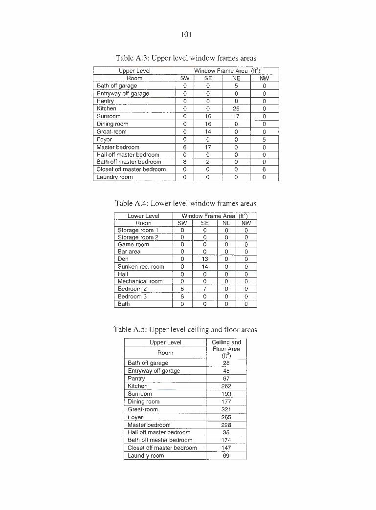
101
Table A.3: Upper level window frames areas
Upper Level Window Frame Area (ft<) Room SW SE NE NW
Bath off garage 0 0 5 0 Entryway off garage 0 0 0 0 Pantry 0 0 0 0 Kitchen 0 0 26 0 Sunroom 0 16 17 0 Dining room 0 16 0 0 Great-room 0 14 0 0 Foyer 0 0 0 5 Master bedroom 6 17 0 0 Hall off master bedroom 0 0 0 0 Bath off master bedroom 8 2 0 0 Closet off master bedroom 0 0 0 6 Laundry room 0 0 0 0
Table A.4: Lower level window frames areas
Lower Level Window Frame Area (ft<) Room SW SE NE NW
Storaqe room 1 0 0 0 0 Storaqe room 2 0 0 0 0 Game room 0 0 0 0 Bar area 0 0 0 0 Den 0 13 0 0 Sunken rec. room 0 14 0 0 Hall 0 0 0 0 Mechanical room 0 0 0 0 Bedroom 2 6 7 0 0 Bedroom 3 8 0 0 0 Bath 0 0 0 0
Table A.5: Upper level ceiling and floor areas
Upper Level Ceiling and
Room Floor Area
(ft2) Bath off garage 28 Entryway off garage 45 Pantry 67 Kitchen 262 Sunroom 193 Dining room 177 Great-room 321 Foyer 265 Master bedroom 228 Hall off master bedroom 35 Bath off master bedroom 174 Closet off master bedroom 147 Laundry room 69

102
Table A.6: Lower level floor and ceiling areas
Lower Level Floor and
Room Ceiling Area
(ft ') Storage room 1 156 Storage room 2 63 Game room 316 Bar area 334 Den 195 Sunken rec. room 556 Hall 141 Mechanical room 56 Bedroom 2 263 Bedroom 3 275 Bath 69
Table A.7: Upper level above grade exterior wall areas
Upper Level Wall (ft2)
Room NE SE SW NW Bath off garage 47 58 0 0 Entryway off garage 23 0 0 0 Pantry 0 0 22 0 Kitchen 41 0 0 0 Sunroom 82 65 20 71 Dining room 0 63 0 0 Great-room 28 161 28 0 Foyer 0 0 47 126 Master bedroom 0 65 147 0 Hall off master bedroom 0 0 0 0 Bath off master bedroom 0 47 112 55 Closet off master bedroom 106 0 98 132 Laundry room 0 0 0 0
Table A.8: Lower level above grade exterior exposed wall areas
Lower Level Wall (ft2)
Room NE SE SW NW Storage room 1 0 0 0 0 Storage room 2 0 0 0 0 Game room 0 0 0 0 Bar area 0 0 0 0 Den 0 59 18 0 Sunken rec. room 19 169 19 0 Hall 0 0 0 0 Mechanical room 0 0 0 0 Bedroom 2 0 112 176 0 Bedroom 3 0 0 132 47 Bath 0 0 0 0

103
Table A.9: Lower level below grade exterior wall areas
Lower Level Wall (ft2)
Room NE SE SW NW Total Storage room 1 101 0 18 132 251 Storage room 2 0 0 82 65 147 Game room 169 48 127 0 345 Bar area 156 0 22 0 178 Den 136 0 0 88 224 Sunken rec. room 0 0 0 0 0 Hall 0 0 0 81 81 Mechanical room 0 0 0 75 75 Bedroom 2 0 0 0 0 0 Bedroom 3 92 0 0 136 229 Bath 0 0 0 0 0
Table A.IO: Upper level exposed partitions to unconditioned space areas
Upper Level Partition (ft2)
Room NE SE SW NW
Bath off garage 0 0 0 58 Entryway off garage 0 0 0 42 Pantry 0 0 0 112 Kitchen 0 0 0 0 Sunroom 0 0 0 0 Dininc::i room 0 0 0 0 Great-room 0 0 0 0 Foyer 0 0 0 0 Master bedroom 0 0 0 0 Hall off master bedroom 0 0 0 0 Bath off master bedroom 0 0 0 0 Closet off master bedroom 0 0 0 0 Laundry room 0 0 0 0
Table A.11: Upper level ceiling height and room volumes
Upper Level Ceiling Volume Room Ht. (ft) (ft3)
Bath off garage 10.1 291 Entryway off garage 10.1 463 Pantry 10.1 684 Kitchen 10.1 2646 Sunroom 10.1 1951 Dining room 10.1 1787 Great-room 14.1 4526 Foyer 11.1 2945 Master bedroom 10.1 2307 Hall off master bedroom 10.1 357 Bath off master bedroom 10.1 1756 Closet off master bedroom 10.1 1490 Laundry room 10.1 702

104
Table A.12: Lower level ceiling height and room volumes
Lower Level Ceiling Ht. Volume Room (ft) (ft3)
Storage room 1 8.8 1368 Storage room 2 8.8 554 Game room 8.8 2778 Bar area 8.8 2936 Den 8.8 1714 Sunken rec. room 10.0 5537 Hall 8.8 1236 Mechanical room 8.8 492 Bedroom 2 8.8 2308 Bedroom 3 8.8 2416 Bath 8.8 604
Table A.13: Upper level rough opening areas
Upper Level Glass and Window (ft2)
Room SW SE NE NW Bath off garage 0 0 12 0 Entryway off garage 0 0 0 0 Pantry 0 0 0 0 Kitchen 0 0 105 0 Sunroom 0 72 72 0 Dining room 0 72 0 0 Great-room 0 111 0 0 Foyer 0 0 0 63 Master bedroom 15 72 0 0 Hall off master bedroom 0 0 0 0 Bath off master bedroom 36 6 0 0 Closet off master bedroom 0 0 0 30 Laundry room 0 0 0 0
Table A.14: Lower level rough opening areas
Lower Level Glass and Window (ft2) Room SW SE NE NW
Storage room 1 0 0 0 0 Storage room 2 0 0 0 0 Game room 0 0 0 0 Bar area 0 0 0 0 Den 0 57 0 0 Sunken rec. room 0 150 0 0 Hall 0 0 0 0 Mechanical room 0 0 0 0 Bedroom 2 15 51 0 0 Bedroom 3 30 0 0 0 Bath 0 0 0 0
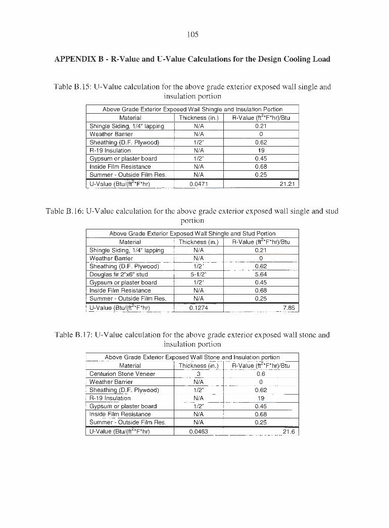
105
APPENDIX B - R-Value and U-Value Calculations for the Design Cooling Load
Table B.15 : U-Value calculation for the above grade exterior exposed wall single and insulation portion
Above Grade Exterior Exposed Wall Shingle and Insulation Portion
Material Thickness (in.) R-Value (tt2*F*hr)/Btu Shingle Siding, 1/4" lapping N/A 0.21 Weather Barrier N/A 0 Sheathing (D.F. Plywood) 1/2" 0.62 R-19 Insulation N/A 19 Gypsum or plaster board 1/2" 0.45 Inside Film Resistance N/A 0.68 Summer - Outside Film Res. N/A 0.25
U-Value (Btu/(ttL*F*hr) 0.0471 21.21
Table B.16: U-Value calculation for the above grade exterior exposed wall single and stud portion
Above Grade Exterior Exposed Wall Shingle and Stud Portion Material Thickness (in.) R-Value (ft2*F*hr)/Btu
Shingle Siding, 1/4" lapping N/A 0.21 Weather Barrier N/A 0 Sheathing (D.F. Plywood) 1/2" 0.62 Douglas fir 2"x6" stud 5-1/2" 5.64 Gypsum or plaster board 1/2" 0.45 Inside Film Resistance N/A 0.68 Summer - Outside Film Res. N/A 0.25
U-Value (Btu/(ft~*F*hr) 0.1274 7.85
Table B.17: U-Value calculation for the above grade exterior exposed wall stone and insulation portion
Above Grade Exterior Exposed Wall Stone and Insulation portion Material Thickness (in.) R-Value (ft2*F*hr)/Btu
Centurion Stone Veneer 3 0.6 Weather Barrier N/A 0 Sheathing (D.F. Plywood) 1/2" 0.62 R-19 Insulation N/A 19 Gypsum or plaster board 1/2" 0.45 Inside Film Resistance N/A 0.68 Summer - Outside Film Res. N/A 0.25
U-Value (Btu/(ft2*F*hr) 0.0463 21 .6

106
Table B.18: U-Value calculation for the above grade exterior exposed wall stone and stud portion
Above Grade Exterior Exposed Wall Stone and Stud Portion
Material Thickness (in.) A-Value (tt2*F*hr)/Btu Centurion Stone Veneer 3" 0.6 Weather Barrier N/A 0 Sheathing (D.F. Plywood) 1/2" 0.62 Douglas fir 2"x6" stud 5-1 /2" 5.64 Gypsum or plaster board 1/2" 0.45 Inside Film Resistance N/A 0.68 Summer - Outside Film Res. N/A 0.25
U-Value (Btu/(ft2*F*hr) 0.1214 8.24
Table B.19: U-Value calculation for the exposed floor on the lower level
Exposed Floor in the Lower Level
Material Thickness (in.) A-Value (ft2*F*hr)/Btu Concrete 4 0.36 Insulation foam board 2 10
U-Value (Btu/(ft"*F*hr) 0.0965 0.36
Table B.20: U-Value calculation for the window frames
Window Frames
Material Thickness (in.) A-Value (tt2*F*hr)/Btu Oak 5 4.225 Inside Film Resistance N/A 0.68 Summer - Outside Film Res. N/A 0.25
U-Value (Btu/(tt"*F*hr) 0.1940 5.16
Table B.21: U-Value calculation for the doors
Doors Material Thickness (in.) A-Value (ft2*F*hr)/Btu
Oak 2 1.69 Inside Film Resistance N/A 0.68 Summer - Outside Film Res. N/A 0.25
U-Value (Btu/(ft2*F*hr) 0.3817 2.62

107
Table B.22: U-Value calculation for the unconditioned partition to the garage insulation portion
Unconditioned Partition to Garage Insulation Portion
Material Thickness (in .) R-Value (ft2*F*hr)/Btu R-19 Insulation N/A 19 Gypsum or plaster board 1/2" 0.45 Gypsum or plaster board 1/2" 0.45 Inside Film Resistance N/A 0.68
U-Value (Btu/(ft2*F*hr) 0.0486 20.58
Table B.23: U-Value calculation for the unconditioned partition to the garage stud portion
Unconditioned Partition to Garage Stud Portion
Material Thickness (in.) R-Value (ft2*F*hr)/Btu Douglas fir 2"x6" stud 5-1 /2" 5.64 Gypsum or plaster board 1/2" 0.45 Gypsum or plaster board 1/2" 0.45 Inside Film Resistance N/A 0.68
U-Value (Btu/(fr' *F*hr) 0.1386 7.22
Table B.24: U-Value calculation for the exterior basement walls below grade insulation portion
Exterior Basement Walls Below Grade Insulation Portion
Material Thickness (in.) R-Value (ft2*F*hr)/Btu Concrete 8 0.72 Insulation N/A 13 Gypsum or plaster board 1/2" 0.45
U-Value (Btu/(ft2*F*hr) 0.0706 14.17
Table B.25: U-Value calculation for the exterior basement walls below grade stud portion
Exterior Basement Walls Below Grade Stud Portion
Material Thickness (in.) R-Value (ft2*F*hr)/Btu Concrete 8 0.72 Douglas fir 2"x4" stud 3-1 /2" 3.59 Gypsum or plaster board 1/2" 0.45
U-Value (Btu/(tt"*F*hr) 0.2102 4.76
Table B.26: U-Value calculation for the upper level below roof insulation portion
Upper Level Ceiling Below Roof Insulation Portion Material Thickness (in .) R-Value (ft2*F*hr)/Btu
Gypsum or plaster board 1/2" 0.45 R-38 Insulation N/A 38 U-Value (Btu/(ft<*F*hr) 0.0260 38.45

108
Table B.27: U-Value calculation for the lower level exterior exposed wall section stone and insulation portion
Lower Level Exterior Exposed Wall Stone and Insulation Portion Material Thickness (in.) R-Value (ft2*F*hr)/Btu
Centurion Stone Veneer 3 0.6 Weather Barrier N/A 0 Sheathing (D.F. Plywood) 1/2" 0.62 R-13 Insulation N/A 13 Gypsum or plaster board 1/2" 0.45 Inside Film Resistance N/A 0.68 Summer - Outside Film Res. N/A 0.25
U-Value (Btu/(ft'*F*hr) 0.0641 15.6
Table B.28: U-Value calculation for the lower level exterior exposed wall section stone and stud portion
Lower Level Exterior Exposed Wall Stone and Stud Portion Material Thickness (in.) R-Value (ft2*F*hr)/Btu
Centurion Stone Veneer 3" 0.6 Weather Barrier N/A 0 Sheathing (D.F. Plywood) 1/2" 0.62 Douglas fir 2"x4" stud 3.5 3.59 Gypsum or plaster board 1/2" 0.45 Inside Film Resistance N/A 0.68 Summer - Outside Film Res. N/A 0.25
U-Value (Btu/(ft' *F*hr) 0.1616 6.19
Table B.29: U-Value calculation for the section between floors insulation portion
Between Floors Wall Section Insulation Portion
Material Thickness (in.) R-Value (ft2*F*hr)/Btu Centurion Stone Veneer 3" 0.6 Sheathing (D.F. Plywood) 1/2" 0.62 Insulation N/A 19 Gypsum or plaster board 1/2" 0.45
U-Value (Btu/(ft2*F*hr) 0.0484 20.67
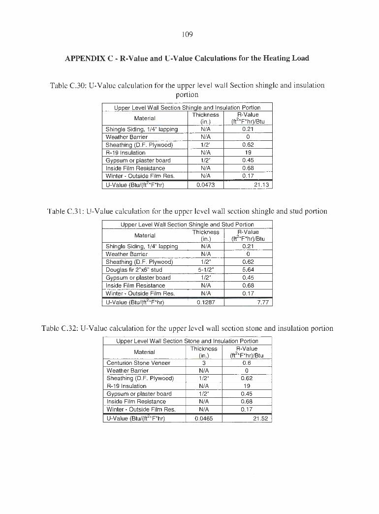
109
APPENDIX C - R-Value and U-Value Calculations for the Heating Load
Table C.30: U-Value calculation for the upper level wall Section shingle and insulation portion
Upper Level Wall Section Shingle and Insulation Portion
Material Thickness R-Value
(in.) (ft2*F*hr)/Btu Shingle Siding, 1/4" lapping N/A 0.21 Weather Barrier N/A 0 Sheathing (D.F. Plywood) 1/2" 0.62 R-19 Insulation N/A 19 Gypsum or plaster board 1/2" 0.45 Inside Film Resistance N/A 0.68 Winter - Outside Film Res. N/A 0.17
U-Value (Btu/(ftL*F*hr) 0.0473 21.13
Table C.31: U-Value calculation for the upper level wall section shingle and stud portion
Upper Level Wall Section Shingle and Stud Portion
Material Thickness R-Value
(in.) (ft2*F*hr)/Btu Shingle Siding, 1 /4" lapping N/A 0.21 Weather Barrier N/A 0 Sheathing (D.F. Plywood) 1/2" 0.62 Douglas fir 2"x6" stud 5-1/2" 5.64 Gypsum or plaster board 1/2" 0.45 Inside Film Resistance N/A 0.68 Winter - Outside Film Res. N/A 0.17
U-Value (Btu/(ftL*F*hr) 0.1287 7.77
Table C.32: U-Value calculation for the upper level wall section stone and insulation portion
Upper Level Wall Section Stone and Insulation Portion
Material Thickness R-Value
(in.) (ft2*F*hr)/Btu Centurion Stone Veneer 3 0.6 Weather Barrier N/A 0 Sheathing (D.F. Plywood) 1/2" 0.62 R-19 Insulation N/A 19 Gypsum or plaster board 1/2" 0.45 Inside Film Resistance N/A 0.68 Winter - Outside Film Res. N/A 0.17
U-Value (Btu/(ft2*F*hr) 0.0465 21 .52
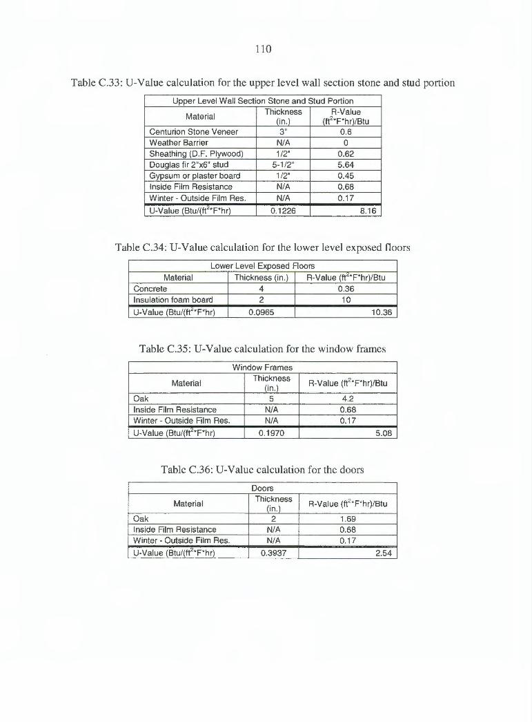
110
Table C.33: U-Value calculation for the upper level wall section stone and stud portion
Upper Level Wall Section Stone and Stud Portion
Material Thickness A-Value
(in .) (ft2*F*hr)/Btu Centurion Stone Veneer 3" 0.6 Weather Barrier N/A 0 Sheathing (D.F. Plywood) 1/2" 0.62 Douglas fir 2"x6" stud 5-1 /2" 5.64 Gypsum or plaster board 1/2" 0.45 Inside Film Resistance N/A 0.68 Winter - Outside Film Res. N/A 0.17
U-Value (Btu/(ft2*F*hr) 0.1226 8.16
Table C.34: U-Value calculation for the lower level exposed floors
Lower Level Exposed Floors
Material Thickness (in.) A-Value (ft2*F*hr)/Btu Concrete 4 0.36 Insulation foam board 2 10
U-Value (Btu/(ft"*F*hr) 0.0965 10.36
Table C.35: U-Value calculation for the window frames
Window Frames
Material Thickness
A-Value (ft2*F*hr)/Btu (in.)
Oak 5 4.2 Inside Film Resistance N/A 0.68 Winter - Outside Film Res. N/A 0.17
U-Value (Btu/(ft2*F*hr) 0.1970 5.08
Table C.36: U-Value calculation for the doors
Doors
Material Thickness
A-Value (ft2*F*hr}/Btu (in.) Oak 2 1.69 Inside Film Resistance N/A 0.68 Winter - Outside Film Res. N/A 0.17
U-Value (Btu/(ft2*F*hr} 0.3937 2.54

111
Table C.37: U-Value calculation for upper level partition to an unconditioned space insulation portion
Upper Level Wall Section to Partition to Garage Insulation Portion
Material Thickness (in.) Fl-Value (ft2*F*hr)/Btu
R-19 Insulation N/A 19 Gypsum or plaster board 1/2" 0.45 Gypsum or plaster board 1/2" 0.45 Inside Film Resistance N/A 0.68
U-Value (Btu/(ft2*F*hr) 0.0486 20.58
Table C.38: U-Value calculation for upper level partition to an unconditioned space stud portion
Upper Level Wall Section Partition to Garage Stud Portion
Material Thickness (in .) Fl-Value (ft2*F*hr)/Btu Douglas fir 2"x6" stud 5-1 /2" 5.64 Gypsum or plaster board 1/2" 0.45 Gypsum or plaster board 1/2" 0.45 Inside Film Resistance N/A 0.68
U-Value (Btu/(ft2*F*hr) 0.1386 7.22
Table C.39: U-Value calculation for lower level exterior below grade wall section insulation portion
Lower Level Wall Section Exterior Below Grade Insulation Portion
Material Thickness (in.) Fl-Value (ft2*F*hr)/Btu Concrete 8 0.72 Insulation N/A 13 Gypsum or plaster board 1/2" 0.45
U-Value (Btu/(ft"*F*hr) 0.0706 14.17
Table C.40: U-Value calculation for lower level exterior below grade wall section stud portion
Lower Level Exterior Below Grade Wall Section Stud Portion Material Thickness (in.) Fl-Value (ft2*F*hr)/Btu
Concrete 8 0.72 Douglas fir 2"x4" stud 3-1 /2" 3.59 Gypsum or plaster board 1/2" 0.45
U-Value (Btu/(ft2*F*hr) 0.2102 4.76
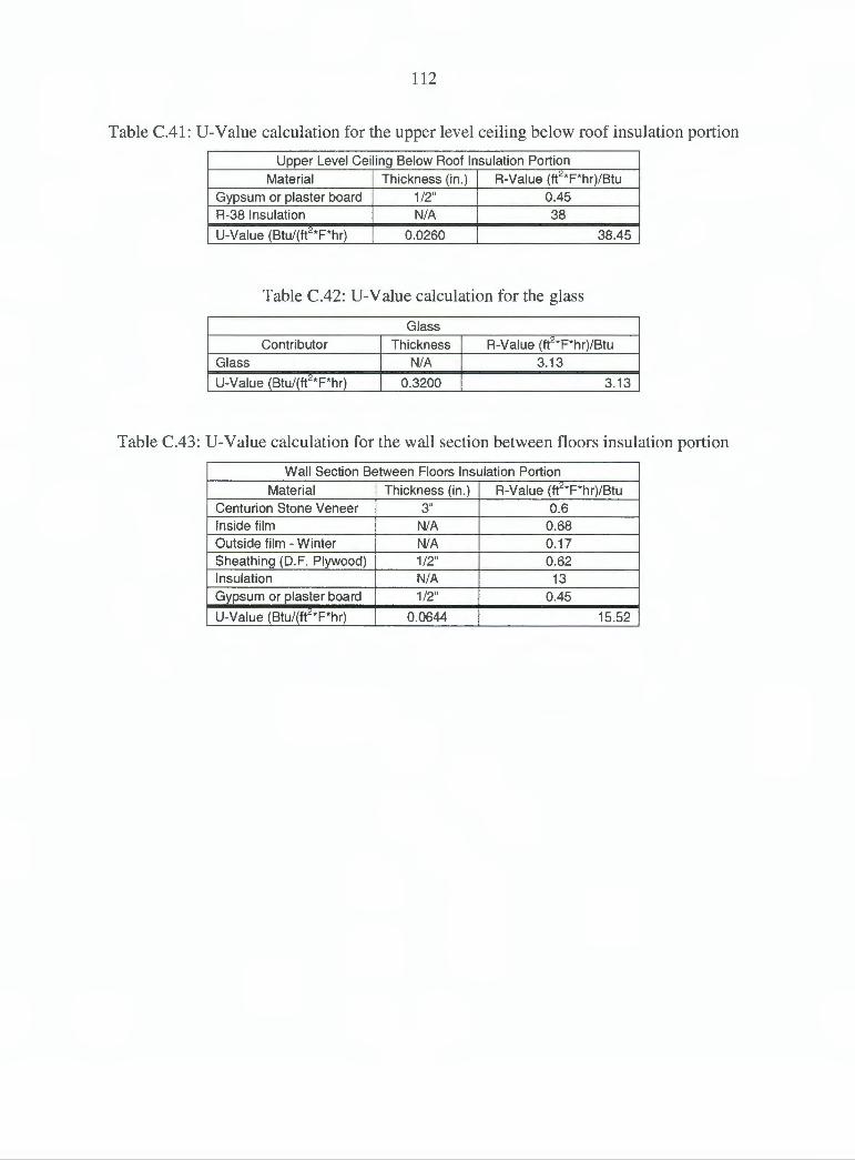
112
Table C.41: U-Value calculation for the upper level ceiling below roof insulation portion
Upper Level Ceiling Below Roof Insulation Portion Material Thickness (in.) A-Value (ft2*F*hr)/Btu
Gypsum or plaster board 1/2" 0.45 R-38 Insulation N/A 38
U-Value (Btu/(ff*F*hr) 0.0260 38.45
Table C.42: U-Value calculation for the glass
Glass Contributor Thickness A-Value (ft2*F*hr)/Btu
Glass N/A 3.13
U-Value (Btu/(ft'*F*hr) 0.3200 3.13
Table C.43: U-Value calculation for the wall section between floors insulation portion
Wall Section Between Floors Insulation Portion
Material Thickness (in.) A-Value (ft2*F*hr)/Btu Centurion Stone Veneer 3" 0.6 Inside film N/A 0.68 Outside film - Winter N/A 0.17 Sheathing (D.F. Plywood) 1/2" 0.62 Insulation N/A 13 Gypsum or plaster board 1/2" 0.45
U-Value (Btu/(ft'*F*hr) 0.0644 15.52
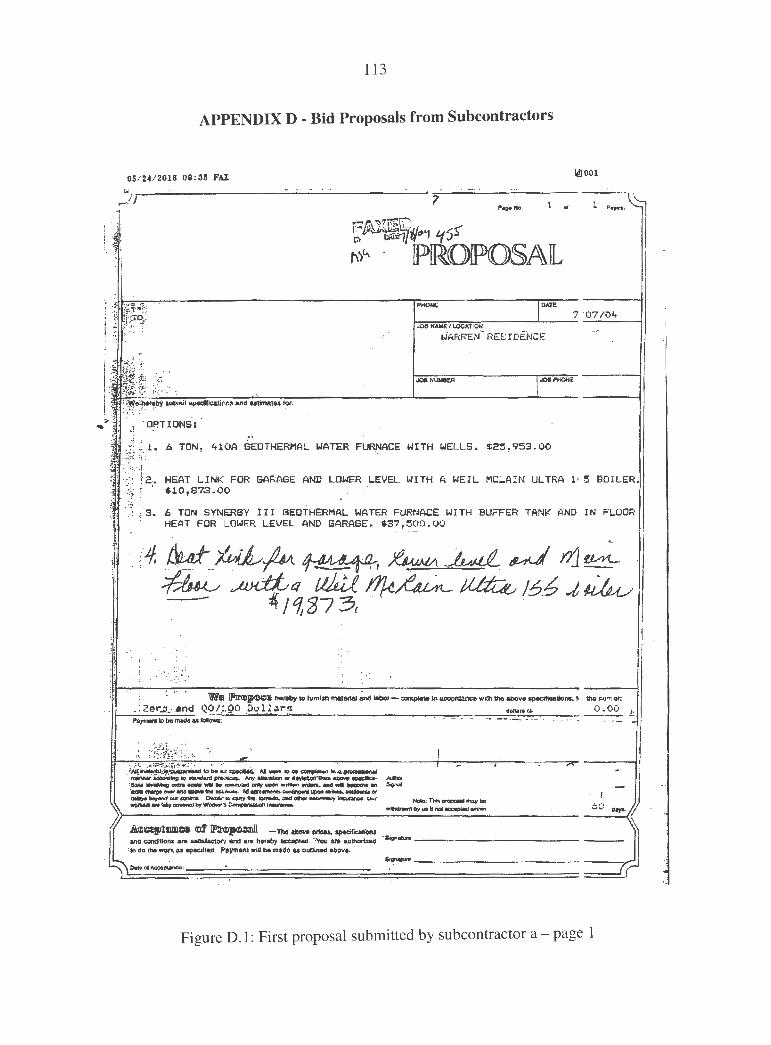
113
APPENDIX D - Bid Proposals from Subcontractors
05 / 24 / 2018 09:35 F..U li!)OOl ,. __ _;, _________ ·..;--· -· -·- ·-··---------::-'-------------.- 7 1 ,, P•a•No
t~~~i/"'1 '1s-r t-i~"' · IPIR.OlPO§Al
; _, lr.::~1~:.•=-.r .,..,-------------~P>IO<l~c-------rl:=;°"'re:;--: ·~ Cf 7 '07 /04 i f JO&HA.Mf l l.OCATION
i - l.J°ARREN~ RESIOE!'JCE
1f1., ::f_ , 1JORP+-40HE
f . [~e:~aby &ubmit apeoifloaliMS and -N kJr. > ,t : •'-f.t ~:: I' · .
,. ;' ,i , OP.TIONS: rir, • TON, 410A 6EOTHERNAL WATER FU~ACE WITH WELLS, •2",9'53.00
1 ·,··• , 2. HEAT LINK FOR GARAGE AND LO~ER LEVEL WITH A WEIL MCLAIN ULTRA l• ~ BOILER :1 · }; f ' $10,873.00
f. ·:.;l::s. c TON SYNERGY III SEOTH~MAL WATER FURNACE WITH BUFFER TANK AND IN FLOOR HEAT FOR LOWER LEVEL ANO GARAGE. $3?,~00.00 .
·: : !" ••. Ve& JPnp~ ~'° tumlah mat•ttal· ~ labor- comp~ ln ae::c:oNlanee with tho abOv• sp•cificellonc, 1, tho -um of:
. : 2er..o.-.and QO/.~QO ,?i;,l la.r~ dollar•<~ 0 .00 ,.
-- ,,c· J .-~;..:::..-:;;:j~ _..,; ; ,. , •. r· · · · ••· · ·-~~~~taMu~ M'MIISIOot~ln--~ · mar'lfWW'•~l.ng19-.n,dm,·~ Mflll .. 18iidn1114!NdoQ"ftmnilboff,....-ca• :uon, ~ ~ ooew war a. ~.cl ontv uoon .,_... ~ and _. "90fflt! an 'Gft~1'Nf"_,.,_,...1Nt&l:tnr;ik. Al--ements~'4)Qr'lllk.._~OC' ._,.e.,a,:a OCM'C!OM'Ol o.wi.r ... qrf)' .... IOMado..ald~~ ~ . Ouf
,,...,,,. --. ··- · -
I I
;\_ ~--W; o:Mntdbr° Wodle(·J. Carnptnal.or1 f~ Hola: Thi• p-QP0,111 ffllly bo
wNrawnO-,ia. not~ .w.n 6 0 daf$-J. \ '/
Mll:IS]pl!UCB Gnf JFN~ -Tho ill)OYII llrioe>. sp,tcillealions and •condftions an &atkUu:torr and.•r• hereby accept.S. 'iYou an .authoriz.a4 -~..--------------- ----
;to do the Wont u apeci.HeJS. F'aym1r\l will be mi-<10 M- outlinlld above. ·
SI~-------- ------~
Figure D. l: First proposal submitted by subcontractor a - page 1

114
05 / 24 / 2016 09:38 FAX
r 1 ' "'-'' i' "'""" dk~'l ~001
!:il52746483 CITY WlI£ i-nTit'6 P(J(; '. 02 . ,
!) ,. ..... ==tL l -' ia.e-,.
l?ROIPOSAL
......... 10,m. :s
5 5/S T0 JCe ..,.we I LOCATIOtl
WARREN RESIDENQ,E
JOBIIII~ 1-----apaoir---•tar.
INSTALLATION OF THE FOLLOUING EgUIPl1ENT:
1- BRYANT 9a~ GAS FU~NACE, l'IOD£L 840MAVOb0120, 120,000 6.T.U.
l - BRYANT 5 TON EVAPORATOR COIL. 1- BRYANT 5 TON, 1e. s.E.E.R • . CONDcNSING UNIT, MODEL 563CNXOb0. 1 - HOIIIEYI.IELL 1-1£:ATING-COOLING PROGf;AMMA!ILE THERMOSTAT. t- APRIL.Al~ l'IODEL o00 HUM,lDIIF'ER.
lNSTALL/:11"10N OF~ NECE::SSARY SHEET MEiAL, REGISTERS. GRILLS, I
·VENT, J3A TH \1El.rT l NG • GAS LINE TO FURNACE, DRYER, RAN6E AND FIREPLACE. LABOR AND MAT~IAL TD Mi:M<E JOB COMPLETE. 90TH LABOR AND MATERIAL TO TME Ht6HE5T QUAL!TV AVAILABLE.
TWENTY '(E.AA. WARRANTY ON HEAT EXCHANGER BY MFS. FIVE VEAR WARRANTY ON COMPRESSOP. B, MF~. FIVE YEAR WARRANTY ON ~RVANT PARTS BY MFG. ONE VEAR UARRJ:WTV ON ALL OTHER PARTS, LABOR AN.I) MATERIAL..
Twelve W. IfllroJ!ICIINI .._I0"""1 .. _,,.,_,.,llb0,--1nacco--UM1-~for
Thou~a.nt!I St!ven Hundred .and 00 /100 Oo l l s1r• .,_..,,. 1, 1e 1 7 ,.-., .. ..-.. -
-Al....,.. ............ ~ ............. M ........ --..ctn lllti ~ ...... ~ ........ ~ ,,,,,,....._ .. __.,.,,..~ ....... ~-- -....,,~ ... ...,, ............ i:wr ,._,_ --- ..,... ... --~ .... .._~_.-_,...,_...,_., N .......... ~ ........ ----~ -
"' =::..~~-:c=...-=..= ...... ~ ...... - 0ur -...CTiaplClpOlal.,.., ..
........ a,, ...... ~~ ( ... ~d~-n.."""""p1ca.....-, _ ___ ,...__,. __ 111,et,v~ ---· ~ "'11o111e •0111 a--. ,a'IIMl\twillbe .....-~ ..-.... ,. ---- .. , .
,/04
~VER ALL
3E OF'
168aTIClf:
IO .00 I
Figure D.2: First proposal submitted by subcontractor a - page 2
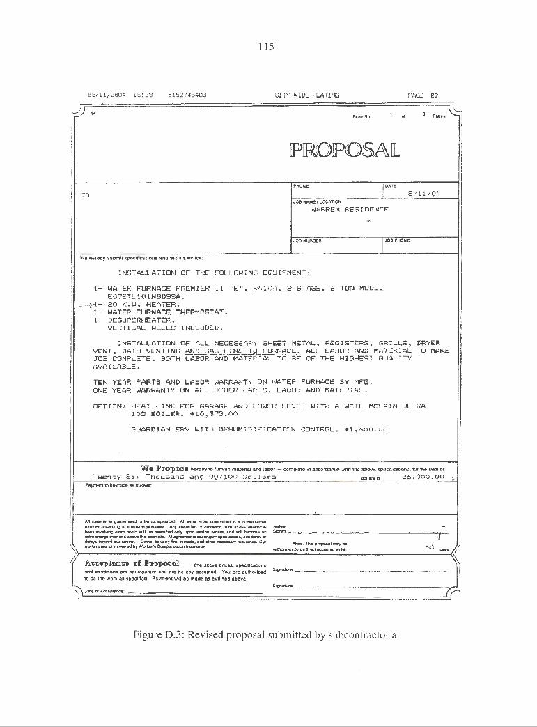
115
08/11/2004 15:39 515274541:13 CITY WIDE HEATING PAGE 02
J it i 1 Page No. ., P1;n-
IPIRO!PO§Al
PHON!!: I om TO 8/11/1)4-
.:oe NAME ' LOCATION
WARREN R.ESlOENCE ;
""
JOB NUMeER 1.10a PHONE
Wa hereby submit ,pocmcauons ana esllmate.s tor;
INSTALLATION OF THE FOLLOWING EC1LI l F"·MENT:
1- WATER FURNACE PREMIER II llEll 'I R410A. 2 STAGE, 6 TON MODEL E072TL101NBDSSA.
-~- 20 K.W. HEATER. 1- WATER FURNACE THERMOSTAT. 1- DESUPERHEATER.
VERTICAL WELLS !NCLUDED.
!NSTALLATION OF ALL NECESSARY SHEET METAL, REGISTERS, GRILLS, DRYER VENT, BATH VENTING AND GAS LINE TQ FURNACE. ALL LABOR ANO MATERlAl TO MAl:'.E JOB COMPLETE. BOTH LABOR AND MtlTERlAL TO BE OF THE HIGHEST QUALITY AVAILABLE.
TEN YEAR PARTS AND LABOR WARRANTY QN ~JATE;;R FURNACE BY MFG, ONE YEAR WARRANTY ON At..L OTHER PARTS, LABOR AND MATERIAL.
OPTIOl'J: HEAT LINK FOR GARAGE AND LDWEF: LEVEL L-JITH A WEIL MCLAIN Ut..TRA 105 BOILER. $10,878.00
GUARDIAN ERV WITH DEHUMIDIFICATION CONTROL. ,u ,600 .00
W/l'JJ lPrr®Jrl®i:111 h<>feby 10 !tJmlah material and labo<- oomple1e ,n am:orttance w1t11 1ho anovo specillcatlol'IO, for the •wn ot:
Twenty Six Thousand and 00/lOCI Dol lars dol lar~ ($ 26,000.00 ),
Peymwtt to be mlll19 u iolkwn:
AB ft'lflleriS! 143 puftfa0teed IO be &i eipecrftlCI. NI WOrk to be compi4Hld In a Dt0'9HJOl'111 mat¥'11M &C;C()f'(ll'OQ 10 ttenoa.rd pr&e:1ie61. A,w Wratlon ot ~bOn ltOm &COltt aaecmca- """"" -tiori, w,\l'Olvin; •xn QOIIU will 1.1b ~ Qnly l,lp0n "ntlcn ord• ns. l:lfld will t,c,,corne an Sq,orn. . mttra d\nrge l:1'4t .and~ 1t1• ..,;m.-. AM ~~t .,.:,a, striJM::::., -'c:1~ or ., dcii,ys bayc::no our corr.rt:11. Ownnr 1D QDfT} frna. tomtido. ind cthw ~ry insura ric;1t. Our Nati,.: This prOfXU'lll may b-9'
~ wurkc,m 819 fuOy --,,cl by Woria,r'o ~ion lnmmsnce,
wttndffn,,,n Z)y Ui II not IICOlptwd 'Wtthiln 60 -•·/, 'I
A<t1:i1Jp>llflllli!:15 QDf IPN~u ~ - Th~ a.cove prtc:.s. speclftcalkms
and conditions af9 se:tit.1aciory and ore hereby accepted. Yoo are authoriz•d 8ig:niltl,INJ'
to do lhe wortc •• specified . PaymMt will oe maoe as oulflnea ab<lv• . $igna1:Yrlf
-.._i O$W Ol ACC:&Ptat\¢e: r
Figure D.3: Revised proposal submitted by subcontractor a

116
• Septics • Trenching
• Back Hoe Work • Waterlines • Mechanical Waste Sytems
• Full Fleet Service Technicians
Ryan & Terry Warren August 18, 2004
RE: Geothermal New Construction WaterFurnace E072 & EW060 Series Installation to Include-
• Set units on pad • New supply plenum • New return drop and
Spacegard air filtration • Duct system for home
(separate supply trunks for up and downstairs), including up to 24-1 st and 20 basement supply runs
• Carrier Comfort Zone 2 zone system
• Bath & Dryer venting • 24v wiring • Condensate to floor drain • 8 ton vertical loop installation • Loop installation does not
include :final grade
Installation Total
• Customer to provide 230v • Desuperheater, connection to
customer's electric water heater
• Customer to have all radiant floor piping in, and Morrell to do all above work for two basement and one garage zone-includes 50 gallon storage tank, all stats, Wirsbo manifolds, and copper piping
• Applicable permits • Installation based on typical
floor joist construction
53,347.00
OPTION NUMBERS __________ _
OPTION SUBTOTAL
TOTAL INSTALLATION PRICE
Thank you for your time and consideration
3
Figure D.4: Proposal submitted by subcontractor b - option 1
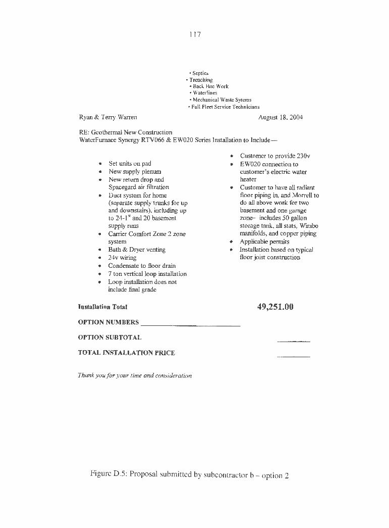
117
• Septics • Trenching
• Back Hoe Work • Waterlines • Mechanical Waste Sytems
• Full Fleet Service Technicians
Ryan & Terry Warren August 18, 2004
RE: Geothermal New Construction WaterFurnace Synergy RTV066 & EW020 Series Installation to Include-
• Set units on pad • New supply plenum • New return drop and
Spacegard air filtration • Duct system for home
(separate supply trunks for up and downstairs), including up to 24- I st and 20 basement supply runs
• Carrier Comfort Zone 2 zone system
• Bath & Dryer venting • 24vwiring • Condensate to floor drain • 7 ton vertical loop installation • Loop installation does not
include final grade
InstaJJation Total
• Customer to provide 230v • EW020 connootion to
customer's electric water heater
• Customer to have all radiant floor piping in, and Morrell to do all above work for two basement and one garage zone-includes 50 gallon storage tank, all stats, Wirsbo manifolds, and copper piping
• Applicable permits • Installation based on typical
floor joist construction
49,251.00
OPTION NUMBERS __________ _
OPTION SUBTOTAL
TOTAL INSTALLATION PRICE
Thank you for your time and consideration
Figure D.5: Proposal submitted by subcontractor b - option 2

118
APPENDIX E - Annual Loan Payments for each Approach
Table E.44: Annual loan payments for approach 1
Approach 1 - E060 & EW040 End Payment Interest
Principal Loan of to Bank
Paid($) Payment Balance
Year ($) ($) ($) 0 $0 $0 $0 $50,000 1 $6,665 $2,800 $3,865 $46,135 2 $6,665 $2,584 $4,082 $42,053 3 $6,665 $2,355 $4,310 $37,743 4 $6,665 $2,114 $4,552 $33,191 5 $6,665 $1 ,859 $4,807 $28,385 6 $6,665 $1 ,590 $5,076 $23,309 7 $6,665 $1 ,305 $5,360 $17,949 8 $6,665 $1 ,005 $5,660 $12,289 9 $6,665 $688 $5,977 $6,312 10 $6,665 $353 $6,312 $0
Total $66,652 $16,652 $50,000 N/A
Table E.45: Annual loan payments for approach 2
Approach 2 - E060 & Electric Boiler End Payment Interest Principal Loan of to Bank Paid($) Payment Balance
Year ($) ($) ($) 0 $0 $0 $0 $35,900 1 $4,786 $2,010 $2,775 $33,125 2 $4,786 $1 ,855 $2,931 $30,194 3 $4,786 $1 ,691 $3,095 $27,099 4 $4,786 $1 ,518 $3,268 $23,831 5 $4,786 $1 ,335 $3,451 $20,380 6 $4,786 $1,141 $3,644 $16,736 7 $4,786 $937 $3,848 $12,887 8 $4,786 $722 $4,064 $8,823 9 $4,786 $494 $4,292 $4,532 10 $4,786 $254 $4,532 $0
Total $47,856 $11 ,956 $35,900 N/A

119
Table E.46: Annual loan payments for approach 3
Ao :,roach 3 - E060 & Liquid Propane Boiler End Payment
Interest Principal Loan
of to Bank Paid($)
Payment Balance Year ($) ($) ($)
0 $0 $0 $0 $37,000 1 $4,932 $2,072 $2,860 $34,140 2 $4,932 $1,912 $3,020 $31,119 3 $4,932 $1,743 $3,190 $27,930 4 $4,932 $1 ,564 $3,368 $24,561 5 $4,932 $1,375 $3,557 $21,005 6 $4,932 $1 ,176 $3,756 $17,249 7 $4,932 $966 $3,966 $13,282 8 $4,932 $744 $4,188 $9,094 9 $4,932 $509 $4,423 $4,671 10 $4,932 $262 $4,671 $0
Total $49,323 $12,323 $37,000 N/A
Table E.47: Annual loan payments for approach 4
Approach 4 - Liquid Propane Boiler, Furnace, Air-Conditioner End Payment Interest Principal of to Bank Paid Payment Loan Balance ($)
Year ($) ($) ($) 0 $0 $0 $0 $23,700 1 $3,159 $1,327 $1,832 $21,868 2 $3,159 $1,225 $1,935 $19,933 3 $3,159 $1 ,116 $2,043 $17,890 4 $3,159 $1 ,002 $2,157 $15,733 5 $3,159 $881 $2,278 $13,454 6 $3,159 $753 $2,406 $11,048 7 $3,159 $619 $2,541 $8,508 8 $3,159 $476 $2,683 $5,825 9 $3,159 $326 $2,833 $2,992 10 $3,159 $168 $2,992 $0
Total $31,593 $7,893 $23,700 N/A

120
APPENDIX F - Annual Operation Costs for each Approach
Table F.48: Annual operation cost for approach 1
Approach 1 - E060 and EW040
Annual Annual Year Year Heating Cooling
Cost($) Cost($) 2004 0 $0 $0 2005 1 $310 $128 2006 2 $310 $128 2007 3 $310 $128 2008 4 $310 $128 2009 5 $310 $128 2010 6 $354 $145 2011 7 $363 $149 2012 8 $375 $154 2013 9 $391 $161 2014 10 $406 $167 2015 11 $419 $172 2016 12 $434 $179 2017 13 $447 $184 2018 14 $462 $190 2019 15 $475 $195 2020 16 $487 $200 2021 17 $506 $208 2022 18 $521 $214 2023 19 $533 $219 2024 20 $552 $227 2025 21 $571 $235 2026 22 $589 $242 2027 23 $608 $250 2028 24 $627 $258 2029 25 $645 $265

121
Table F.49: Annual operation cost for approach 2
Approach 2 - E060 and Electric Boiler
Annual Annual Year Year Heating Cooling
Cost($) Cost($) 2004 0 $0 $0 2005 1 $616 $128 2006 2 $616 $128 2007 3 $616 $128 2008 4 $616 $128 2009 5 $616 $128 2010 6 $616 $145 2011 7 $702 $149 2012 8 $721 $154 2013 9 $746 $161 2014 10 $776 $167 2015 11 $807 $172 2016 12 $832 $179 2017 13 $863 $184 2018 14 $887 $190 2019 15 $918 $195 2020 16 $943 $200 2021 17 $967 $208 2022 18 $1 ,004 $214 2023 19 $1,035 $219 2024 20 $1 ,060 $227 2025 21 $1 ,097 $235 2026 22 $1 ,134 $242 2027 23 $1,171 $250 2028 24 $1,208 $258 2029 25 $1,245 $265

122
Table F.50: Annual operation cost for approach 3
Approach 3 - E060 and Liquid Propane Boiler
Year Year Annual Heating Annual Cooling Cost($) Cost($)
2004 0 $0 $0 2005 1 $719 $128 2006 2 $663 $128 2007 3 $658 $128 2008 4 $678 $128 2009 5 $694 $128 2010 6 $714 $145 2011 7 $759 $149 2012 8 $790 $154 2013 9 $819 $161 2014 10 $850 $167 2015 11 $881 $172 2016 12 $915 $179 2017 13 $951 $184 2018 14 $985 $190 2019 15 $1 ,016 $195 2020 16 $1 ,049 $200 2021 17 $1,083 $208 2022 18 $1 ,126 $214 2023 19 $1 ,162 $219 2024 20 $1,196 $227 2025 21 $1,239 $235 2026 22 $1 ,283 $242 2027 23 $1 ,326 $250 2028 24 $1,369 $258 2029 25 $1,412 $265
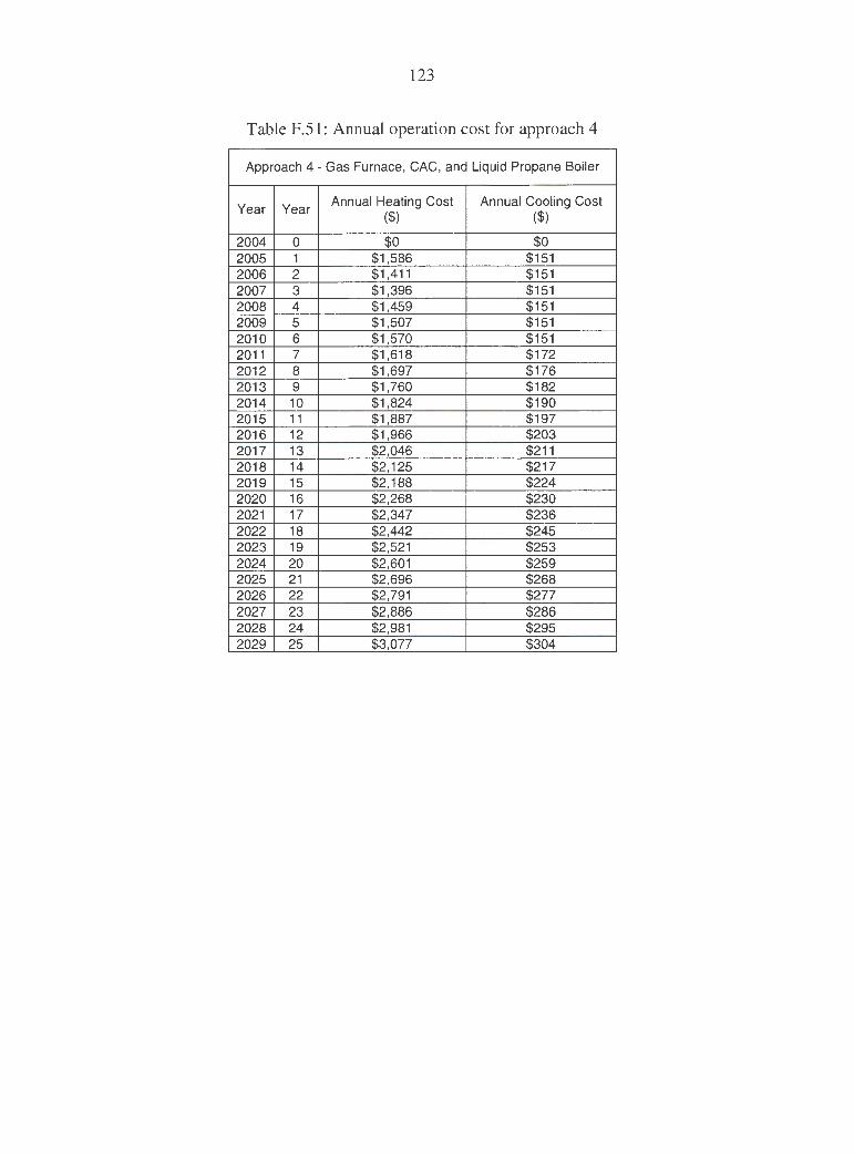
123
Table F.51: Annual operation cost for approach 4
Approach 4 - Gas Furnace, CAC, and Liquid Propane Boiler
Year Year Annual Heating Cost Annual Cooling Cost
($) ($)
2004 0 $0 $0 2005 1 $1,586 $151 2006 2 $1 ,411 $151 2007 3 $1 ,396 $151 2008 4 $1,459 $151 2009 5 $1 ,507 $151 2010 6 $1 ,570 $151 2011 7 $1 ,618 $172 2012 8 $1 ,697 $176 2013 9 $1 ,760 $182 2014 10 $1,824 $190 2015 11 $1 ,887 $197 2016 12 $1 ,966 $203 2017 13 $2,046 $211 2018 14 $2,125 $217 2019 15 $2,188 $224 2020 16 $2,268 $230 2021 17 $2,347 $236 2022 18 $2,442 $245 2023 19 $2,521 $253 2024 20 $2,601 $259 2025 21 $2,696 $268 2026 22 $2,791 $277 2027 23 $2,886 $286 2028 24 $2,981 $295 2029 25 $3,077 $304

124
APPENDIX G - Annual Tax Savings for each Approach
Table G.52: Annual tax savings for approach 1
Approach 1 - E060 & EW040
End of Tax Tax Savings
Year Savings Compared to
($) Conventional ($) 0 $0 $0 1 $1,260 $663 2 $1,163 $612 3 $1 ,060 $557 4 $951 $500 5 $836 $440 6 $715 $376 7 $587 $309 8 $452 $238 9 $310 $163 10 $159 $84
Total $7,494 $3,942
Table G.53: Annual tax savings for approach 2
Approach 2 - E060 & Electric Boiler
End of Tax Tax Savings
Year Savings Compared to
($) Conventional ($) 0 $0 $0 1 $905 $307 2 $835 $284 3 $761 $259 4 $683 $232 5 $601 $204 6 $514 $175 7 $422 $143 8 $325 $110 9 $222 $76 10 $114 $39
Total $5,380 $1,828

125
Table G.54: Annual tax savings for approach 3
Approach 3 - E060 & Liquid Propane Boiler
End of Tax Tax Savings
Year Savings Compared to
($) Conventional ($) 0 $0 $0 1 $932 $335 2 $860 $309 3 $784 $282 4 $704 $253 5 $619 $222 6 $529 $190 7 $435 $156 8 $335 $120 9 $229 $82 10 $118 $42
Total $5,545 $1,993
Table G.55: Annual tax savings for approach 4
Approach 4 - Liquid Propane Boiler, Liquid Propane Furnace, Air-Conditioner
End of Tax Savings ($)
Tax Savings Compared to Year Conventional ($)
0 $0 N/A 1 $597 N/A 2 $551 N/A 3 $502 N/A 4 $451 N/A 5 $396 N/A 6 $339 N/A 7 $278 N/A 8 $214 N/A 9 $147 N/A 10 $75 N/A
Total $3,552 N/A

126
APPENDIX H - Annual Operation Savings for each Approach
Table H.56: Annual Operation Savings for each approach in comparison to conventional ( approach 4)
Annual Operation Savings Compared to Conventional Approach
Approach 1 Approach 2 Approach 3
Year Year Heating and Heating and Heating and
Cooling Savings Cooling Savings Cooling Savings ($) ($) ($)
2004 0 $0 $0 $0 2005 1 $1 ,299 $993 $890 2006 2 $1 ,124 $818 $771 2007 3 $1 ,108 $802 $761 2008 4 $1, 172 $866 $804 2009 5 $1 ,219 $913 $836 2010 6 $1 ,222 $959 $861 2011 7 $1 ,277 $938 $881 2012 8 $1 ,343 $998 $928 2013 9 $1 ,391 $1 ,036 $962 2014 10 $1,440 $1 ,070 $996 2015 11 $1,493 $1 ,105 $1 ,031 2016 12 $1 ,557 $1 ,159 $1,076 2017 13 $1 ,626 $1,210 $1,122 2018 14 $1 ,690 $1,264 $1,167 2019 15 $1 ,743 $1 ,300 $1,202 2020 16 $1 ,811 $1,355 $1,248 2021 17 $1 ,870 $1,408 $1 ,292 2022 18 $1 ,952 $1 ,469 $1,347 2023 19 $2,022 $1 ,520 $1,393 2024 20 $2,081 $1 ,573 $1,436 2025 21 $2,158 $1 ,632 $1,490 2026 22 $2,236 $1 ,692 $1,543 2027 23 $2,314 $1,752 $1,596 2028 24 $2,392 $1 ,811 $1 ,650 2029 25 $2,470 $1 ,871 $1 ,703

End of
Year
0 1 2 3 4 5 6 7 8 9 10 11 12 13 14 15 16 17 18 19 20 21 22 23 24 25
Total
127
APPENDIX I - Present Value Analysis for each Approach
Table I.57: Annual present values for the net cash flow and overall present worth of the system for approach 1
Annual Annual Annual Annual Annual
Payment to Rebate Heating Cost Cooling
Annual Tax Expenses Savings
Present Bank for Loan ($)
($) Cost($) Savings($)
($) ($) Value($)
($) $0 $2,400 $0 $0 $0 $0 $2,400 $2,400
$6,665 $0 $310 $128 $1,260 $7,103 $1 ,961 -$5,591 $6,665 $0 $310 $128 $1,163 $7,103 $1,736 -$5,440 $6,665 $0 $310 $128 $1 ,060 $7,103 $1 ,666 -$5,296 $6,665 $0 $310 $128 $951 $7,103 $1 ,672 -$5,159 $6,665 $0 $310 $128 $836 $7,103 $1,659 -$5,029 $6,665 $0 $354 $145 $715 $7,164 $1 ,598 -$4,952 $6,665 $0 $363 $149 $587 $7,177 $1,586 -$4,843 $6,665 $0 $375 $154 $452 $7,195 $1,581 -$4,741 $6,665 $0 $391 $161 $310 $7,217 $1,554 -$4,648 $6,665 $0 $406 $167 $159 $7,239 $1,524 -$4,559
$0 $0 $419 $172 $0 $591 $1,493 -$364 $0 $0 $434 $179 $0 $613 $1 ,557 -$361 $0 $0 $447 $184 $0 $630 $1 ,626 -$356 $0 $0 $462 $190 $0 $652 $1,690 -$352 $0 $0 $475 $195 $0 $670 $1,743 -$346 $0 $0 $487 $200 $0 $687 $1 ,811 -$340 $0 $0 $506 $208 $0 $714 $1 ,870 -$338 $0 $0 $521 $214 $0 $735 $1,952 -$333 $0 $0 $533 $219 $0 $753 $2,022 -$326 $0 $0 $552 $227 $0 $779 $2,081 -$323 $0 $0 $571 $235 $0 $806 $2,158 -$320 $0 $0 $589 $242 $0 $832 $2,236 -$316 $0 $0 $608 $250 $0 $858 $2,314 -$312 $0 $0 $627 $258 $0 $884 $2,392 -$307 $0 $0 $645 $265 $0 $911 $2,470 -$303
$66,652 $2,400 $11 ,315 $4,655 $7,494 $82,623 $48,353 -$52,854
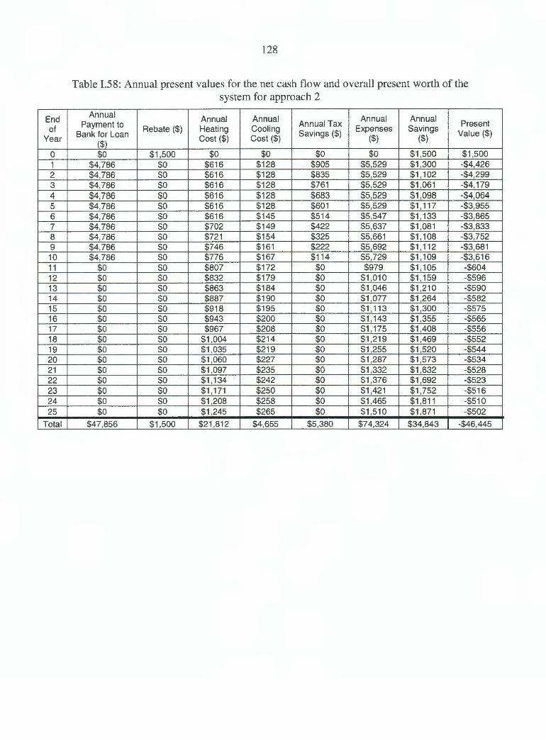
End of
Year
0 1 2 3 4 5 6 7 8 9 10 11 12 13 14 15 16 17 18 19 20 21 22 23 24 25
Total
128
Table 1.58: Annual present values for the net cash flow and overall present worth of the system for approach 2
Annual Annual Annual Annual Annual Payment to
Rebate($) Heating Cooling Annual Tax
Expenses Savings Present
Bank for Loan Cost($) Cost($) Savings($)
($) ($) Value($)
($) $0 $1 ,500 $0 $0 $0 $0 $1 ,500 $1,500
$4,786 $0 $616 $128 $905 $5,529 $1 ,300 -$4,426 $4,786 $0 $616 $128 $835 $5,529 $1 ,102 -$4,299 $4,786 $0 $616 $128 $761 $5,529 $1 ,061 -$4,179 $4,786 $0 $616 $128 $683 $5,529 $1,098 -$4,064 $4,786 $0 $616 $128 $601 $5,529 $1,117 -$3,955 $4,786 $0 $616 $145 $514 $5,547 $1 ,133 -$3,865 $4,786 $0 $702 $149 $422 $5,637 $1 ,081 -$3,833 $4,786 $0 $721 $154 $325 $5,661 $1 ,108 -$3,752 $4,786 $0 $746 $161 $222 $5,692 $1,112 -$3,681 $4,786 $0 $776 $167 $114 $5,729 $1 ,109 -$3,616
$0 $0 $807 $172 $0 $979 $1 ,105 -$604 $0 $0 $832 $179 $0 $1 ,010 $1,159 -$596 $0 $0 $863 $184 $0 $1,046 $1 ,210 -$590 $0 $0 $887 $190 $0 $1,077 $1,264 -$582 $0 $0 $918 $195 $0 $1 ,113 $1 ,300 -$575 $0 $0 $943 $200 $0 $1 ,143 $1 ,355 -$565 $0 $0 $967 $208 $0 $1 ,175 $1,408 -$556 $0 $0 $1 ,004 $214 $0 $1 ,219 $1,469 -$552 $0 $0 $1 ,035 $219 $0 $1 ,255 $1 ,520 -$544 $0 $0 $1 ,060 $227 $0 $1,287 $1 ,573 -$534 $0 $0 $1,097 $235 $0 $1 ,332 $1,632 -$528 $0 $0 $1,134 $242 $0 $1 ,376 $1 ,692 -$523 $0 $0 $1 , 171 $250 $0 $1,421 $1 ,752 -$516 $0 $0 $1 ,208 $258 $0 $1,465 $1 ,811 -$510 $0 $0 $1 ,245 $265 $0 $1 ,510 $1,871 -$502
$47,856 $1,500 $21,812 $4,655 $5,380 $74,324 $34,843 -$46,445

End of
Year
0 1 2 3 4 5 6 7 8 9 10 11 12 13 14 15 16 17 18 19 20 21 22 23 24 25
Total
129
Table I.59: Annual present values for the net cash flow and overall present worth of the system for approach 3
Annual Annual Annual Annual Annual
Payment to Rebate($) Heating Cooling
Annual Tax Expenses Savings
Present Bank for Loan
Cost($) Cost($) Savings($)
($) ($) Value($)
($) $0 $1 ,500 $0 $0 $0 $0 $1,500 $1,500
$4,932 $0 $719 $128 $932 $5,779 $1,225 -$4,638 $4,932 $0 $663 $128 $860 $5,723 $1 ,081 -$4,453 $4,932 $0 $658 $128 $784 $5,718 $1,042 -$4,323 $4,932 $0 $678 $128 $704 $5 ,738 $1,057 -$4,222 $4,932 $0 $694 $128 $619 $5,754 $1 ,058 -$4, 120 $4,932 $0 $714 $145 $529 $5,792 $1 ,051 -$4,041 $4,932 $0 $759 $149 $435 $5,840 $1,038 -$3,972 $4,932 $0 $790 $154 $335 $5,877 $1 ,048 -$3,897 $4,932 $0 $819 $161 $229 $5,912 $1,045 -$3,824 $4,932 $0 $850 $167 $118 $5,950 $1,039 -$3,755
$0 $0 $881 $172 $0 $1 ,053 $1,031 -$649 $0 $0 $915 $179 $0 $1,093 $1,076 -$645 $0 $0 $951 $184 $0 $1 ,135 $1,122 -$640 $0 $0 $985 $190 $0 $1 ,175 $1 ,167 -$634 $0 $0 $1 ,016 $195 $0 $1,211 $1,202 -$626 $0 $0 $1 ,049 $200 $0 $1 ,250 $1,248 -$618 $0 $0 $1 ,083 $208 $0 $1,291 $1,292 -$611 $0 $0 $1,126 $214 $0 $1 ,341 $1,347 -$607 $0 $0 $1,162 $219 $0 $1,382 $1,393 -$599 $0 $0 $1 ,196 $227 $0 $1,423 $1,436 -$590 $0 $0 $1,239 $235 $0 $1,474 $1,490 -$585 $0 $0 $1,283 $242 $0 $1,525 $1,543 -$579 $0 $0 $1,326 $250 $0 $1 ,576 $1 ,596 -$573 $0 $0 $1,369 $258 $0 $1,627 $1,650 -$566 $0 $0 $1,412 $265 $0 $1,678 $1,703 -$558
$49,323 $1 ,500 $24,339 $4,655 $5,545 $78,317 $32,481 -$48,826

End of
Year
0 1 2 3 4 5 6 7 8 9 10 11 12 13 14 15 16 17 18 19 20 21 22 23 24 25
Total
130
Table I.60: Annual present values for the net cash flow and overall present worth of the system for approach 4
Annual Annual Annual Annual Annual Payment to Rebate($) Heating Cooling Annual Tax Expenses Savings
Present Bank for Loan Cost($) Cost($)
Savings($) ($) ($) Value($)
($) $0 $0 $0 $0 $0 $0 $0 $0
$3,159 $0 $1,586 $151 $597 $4,896 $0 -$4, 113 $3,159 $0 $1,411 $151 $551 $4,721 $0 -$3,819 $3,159 $0 $1,396 $151 $502 $4,705 $0 -$3,683 $3,159 $0 $1,459 $151 $451 $4,769 $0 -$3,621 $3,159 $0 $1,507 $151 $396 $4,816 $0 -$3,547 $3,159 $0 $1 ,570 $151 $339 $4,880 $0 -$3,487 $3,159 $0 $1 ,618 $172 $278 $4,949 $0 -$3,432 $3,159 $0 $1 ,697 $176 $214 $5,032 $0 -$3,388 $3,159 $0 $1,760 $182 $147 $5,102 $0 -$3,334 $3,159 $0 $1,824 $190 $75 $5,173 $0 -$3,282
$0 $0 $1,887 $197 $0 $2,084 $0 -$1 ,284 $0 $0 $1 ,966 $203 $0 $2,170 $0 -$1,279 $0 $0 $2,046 $211 $0 $2,257 $0 -$1,273 $0 $0 $2,125 $217 $0 $2,342 $0 -$1,265 $0 $0 $2,188 $224 $0 $2,413 $0 -$1 ,247 $0 $0 $2,268 $230 $0 $2,498 $0 -$1 ,235 $0 $0 $2,347 $236 $0 $2,583 $0 -$1,222 $0 $0 $2,442 $245 $0 $2,688 $0 -$1,217 $0 $0 $2,521 $253 $0 $2,775 $0 -$1,202 $0 $0 $2,601 $259 $0 $2,860 $0 -$1, 186 $0 $0 $2,696 $268 $0 $2,964 $0 -$1,176 $0 $0 $2,791 $277 $0 $3,068 $0 -$1, 165 $0 $0 $2,886 $286 $0 $3,172 $0 -$1 , 153 $0 $0 $2,981 $295 $0 $3,277 $0 -$1,139 $0 $0 $3,077 $304 $0 $3,381 $0 -$1, 125
$31,593 $0 $52,650 $5,331 $3,552 $89,575 $0 -$53,876

131
APPENDIX J - Equipment Specifications for WaterFurnace Heat Pump
SIDE VIEW
J_j +-- J ----1
I • K
I -
MODEL WATER
CONNECTION
E036, E040, E047, E048, 1.00" Swivel
E058. E060, E066. E072
LEFT-HAND RETURN AIR
AUX HEAT KNOCKOUTS
1-3/8"
A B C D
31.2 25.5 58.4 18.0
RIGHT-HAND RETURN AIR
E F G
18.0 6.6 6.5
Figure J.6: Vertical configuration dimensional data Source: W aterFurnace, 2004d
H I J K
3.7 1.1 27.3 34.0
L
1.7
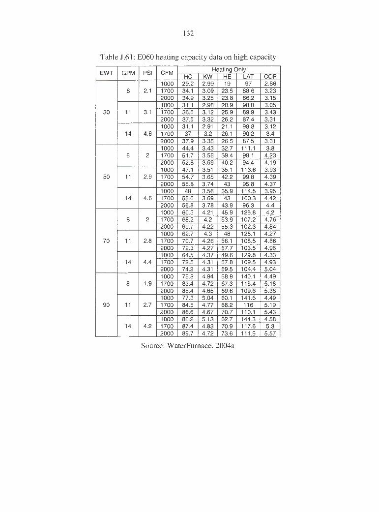
132
Table J.61: E060 heating capacity data on high capacity
EWT GPM PSI CFM Heating Only HC KW HE LAT COP
1000 29.2 2.99 19 97 2.86 8 2.1 1700 34.1 3.09 23.5 88.6 3.23
2000 34.9 3.25 23.8 86.2 3.15 1000 31.1 2.98 20.9 98.8 3.05
30 11 3.1 1700 36.5 3.12 25.9 89.9 3.43 2000 37.5 3.32 26.2 87.4 3.31 1000 31.1 2.91 21 .1 98.8 3.12
14 4.8 1700 37 3.2 26.1 90.2 3.4 2000 37.9 3.35 26.5 87.5 3.31 1000 44.4 3.43 32.7 111 .1 3.8
8 2 1700 51 .7 3.58 39.4 98.1 4.23 2000 52.8 3.69 40.2 94.4 4.19 1000 47.1 3.51 35.1 113.6 3.93
50 11 2.9 1700 54.7 3.65 42.2 99.8 4.39 2000 55.8 3.74 43 95.8 4.37 1000 48 3.56 35.9 114.5 3.95
14 4.6 1700 55.6 3.69 43 100.3 4.42 2000 56.8 3.78 43.9 96.3 4.4 1000 60.3 4.21 45.9 125.8 4.2
8 2 1700 68.2 4.2 53.9 107.2 4.76 2000 69.7 4.22 55.3 102.3 4.84 1000 62.7 4.3 48 128.1 4.27
70 11 2.8 1700 70.7 4.26 56.1 108.5 4.86 2000 72.3 4.27 57.7 103.5 4.96 1000 64.5 4.37 49.6 129.8 4.33
14 4.4 1700 72.5 4.31 57.8 109.5 4.93 2000 74.2 4.31 59.5 104.4 5.04 1000 75.8 4.94 58.9 140.1 4.49
8 1.9 1700 83.4 4.72 67.3 115.4 5.18 2000 85.4 4.65 69.6 109.6 5.38 1000 77.3 5.04 60.1 141 .6 4.49
90 11 2.7 1700 84.5 4.77 68.2 116 5.19 2000 86.6 4.67 70.7 110.1 5.43 1000 80.2 5.13 62.7 144.3 4.58
14 4.2 1700 87.4 4.83 70.9 117.6 5.3 2000 89.7 4.72 73.6 111 .5 5.57
Source: WaterFurnace, 2004a

133
Table J .62: E060 heating capacity data on low capacity
EWT GPM PSI CFM HeatinQ Only
HG KW HE LAT COP 700 16.2 1.5 11 91.4 3.16
5 1.1 900 16.9 1.52 11 .7 87.4 3.27 1100 17.5 1.54 12.3 84.7 3.34 700 16.1 1.53 10.8 91 .2 3.08
30 8 2.1 900 16.8 1.54 11 .5 87.3 3.18 1100 17.4 1.56 12 84.6 3.26 700 16.7 1.53 11.5 92.1 3.2
11 3.1 900 17.4 1.54 12.2 87.9 3.31 1100 18 1.56 12.7 85.2 3.39 700 24.7 1.63 19.2 102.7 4.45
5 1 900 25.9 1.62 20.4 96.6 4.67 1100 26.6 1.62 21.1 92.4 4.81 700 25.1 1.66 19.4 103.2 4.43
50 8 2 900 26.3 1.65 20.6 97 4.67 1100 26.9 1.64 21.3 92.6 4.8 700 25.9 1.67 20.2 104.2 4.54
11 2.9 900 27.1 1.66 21.4 97.9 4.79 1100 27.7 1.65 22.1 93.3 4.92 700 33.6 1.82 27.4 114.4 5.42
5 0.9 900 35.2 1.78 29.2 106.3 5.79 1100 35.8 1.75 29.8 100.1 5.98 700 34.9 1.85 28.6 116.2 5.54
70 8 2 900 36.7 1.81 30.5 107.7 5.95 1100 37.1 1.77 31 .1 101.2 6.13 700 35.6 1.87 29.3 117.1 5.58
11 2.8 900 37.4 1.83 31.2 108.5 6 1100 37.8 1.79 31.7 101 .8 6.19 700 41 1.97 34.3 124.3 6.1
5 0.9 900 43.1 1.9 36.6 114.3 6.63 1100 43.2 1.85 36.9 106.4 6.85 700 43.8 2 37 128 6.42
90 8 1.9 900 46 1.93 39.5 117.4 7 1100 46 1.86 39.7 108.7 7.24 700 44.1 2.04 37.2 128.4 6.34
11 2.7 900 46.3 1.96 39.7 117.7 6.93 1100 46.2 1.89 39.8 108.9 7.17
Source: W aterFurnace, 2004a
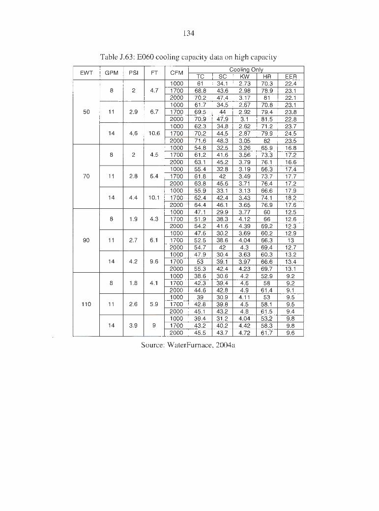
134
Table J.63: E060 cooling capacity data on high capacity
EWT GPM PSI FT CFM Cooling Only TC SC KW HR EER
1000 61 34.1 2.73 70.3 22.4 8 2 4.7 1700 68.8 43.6 2.98 78.9 23.1
2000 70.2 47.4 3.17 81 22.1 1000 61.7 34.5 2.67 70.8 23.1
50 11 2.9 6.7 1700 69.5 44 2.92 79.4 23.8 2000 70.9 47.9 3.1 81.5 22.8 1000 62.3 34.8 2.62 71 .2 23.7
14 4.6 10.6 1700 70.2 44.5 2.87 79.9 24.5 2000 71 .6 48.3 3.05 82 23.5 1000 54.8 32.5 3.26 65.9 16.8
8 2 4.5 1700 61.2 41.6 3.56 73.3 17.2 2000 63.1 45.2 3.79 76.1 16.6 1000 55.4 32.8 3.19 66.3 17.4
70 11 2.8 6.4 1700 61.8 42 3.49 73.7 17.7 2000 63.8 45.6 3.71 76.4 17.2 1000 55.9 33.1 3.13 66.6 17.9
14 4.4 10.1 1700 62.4 42.4 3.43 74.1 18.2 2000 64.4 46.1 3.65 76.9 17.6 1000 47.1 29.9 3.77 60 12.5
8 1.9 4.3 1700 51.9 38.3 4.12 66 12.6 2000 54.2 41.6 4.39 69.2 12.3 1000 47.6 30.2 3.69 60.2 12.9
90 11 2.7 6.1 1700 52.5 38.6 4.04 66.3 13 2000 54.7 42 4.3 69.4 12.7 1000 47.9 30.4 3.63 60.3 13.2
14 4.2 9.6 1700 53 39.1 3.97 66.6 13.4 2000 55.3 42.4 4.23 69.7 13.1 1000 38.6 30.6 4.2 52.9 9.2
8 1.8 4.1 1700 42.3 39.4 4.6 58 9.2 2000 44.6 42.8 4.9 61.4 9.1 1000 39 30.9 4.11 53 9.5
110 11 2.6 5.9 1700 42.8 39.8 4.5 58.1 9.5 2000 45.1 43.2 4.8 61 .5 9.4 1000 39.4 31.2 4.04 53.2 9.8
14 3.9 9 1700 43.2 40.2 4.42 58.3 9.8 2000 45.5 43.7 4.72 61.7 9.6
Source: WaterFumace, 2004a

135
Table J.64: E060 cooling capacity data on low capacity
EWT GPM PSI FT CFM Coolinq Only
TC SC KW HR EER 700 35.3 20.6 1.07 38.9 32.8
5 1 2.3 900 37.6 23.6 1.1 41 .3 34.2 1100 38.7 26.8 1.16 42.7 33.5 700 35.3 20.8 1.03 38.9 34.2
50 8 2 4.6 900 37.7 23.8 1.06 41.3 35.6 1100 38.8 27 1.11 42.6 34.9 700 35.4 20.8 1.01 38.9 35
11 2.9 6.7 900 37.8 23.8 1.04 41.3 36.5 1100 38.9 27 1.09 42.7 35.7 700 30.8 19.9 1.41 35.6 21.9
5 0.9 2.2 900 32.3 22.3 1.43 37.2 22.6 1100 33.3 25 1.49 38.4 22.4 700 31 20.1 1.36 35.6 22.7
70 8 2 4.6 900 32.5 22.5 1.39 37.2 23.4 1100 33.5 25.3 1.45 38.4 23.2 700 31 .2 20.2 1.34 35.7 23.3
11 2.8 6.4 900 32.7 22.6 1.36 37.3 24 1100 33.7 25.4 1.42 38.5 23.7 700 26.2 19 1.74 32.1 15.1
5 0.9 2.1 900 27 20.8 1.76 33 15.3 1100 27.8 23.1 1.81 34 15.3 700 26.4 19.2 1.7 32.2 15.5
90 8 1.9 4.4 900 27.3 21 1.72 33.2 15.8 1100 28.1 23.4 1.78 34.2 15.8 700 26.7 19.4 1.68 32.4 15.9
11 2.7 6.1 900 27.5 21.2 1.7 33.3 16.2 1100 28.4 23.6 1.75 34.4 16.2 700 21 .7 17.8 2.02 28.6 10.7
5 0.9 2 900 22 19.2 2.04 29 10.8 1100 22.7 21.1 2.08 29.8 10.9 700 22 18 2 28.8 11
110 8 1.8 4.2 900 22.3 19.4 2.02 29.2 11.1 1100 23 21.3 2.06 30 11.2 700 22.3 18.3 1.97 29 11.3
11 2.6 . ·5.9 900 22.6 19.7 1.99 29.4 11.4 1100 23.3 21 .6 2.03 30.3 11 .5
Source: WaterFurnace, 2004a

136
APPENDIX K - Equipment Specifications for Electric Boiler
4 mounting l1oles 9 1 /2" I '""~'""""""~ ~
Combined Temperature and
pressure gauge
-
Dual-Energy Controller (Dual-Energy models only)
Thermostat. connection
--~ -18"
Pressure relief vatve 314" NPT
lnlet 1-114" NPT _ _ _ _ _ __. 1B" -----~ L-----Figure K.7: Physical dimensions of electric boiler
Source: Thermolec, 2004
Pump relay
Electrical supply

137
APPENDIX L - Degree-Day Method
The degree-day method was performed to estimate the annual energy use for the case
study home. The degree-day method is the simplest method evaluated in this study.
Generally, this method is only recommended to estimate energy demands of a single-family
residential home. However, studies have shown that the degree-day analysis may result in
inaccurate estimations and caution a practitioner from using this method. Nevertheless, the
method will be demonstrated to illustrate the differences in results to the bin and improved
methods for annual energy use.
The degree-day method is based on heating degree days and cooling degree days.
The number of degree days for a particular location is the measure of departure from a given
standard (usually 65°F), one degree day for each degree of departure either above or below
the standard during one day. To calculate the number of degree days that could be seen at
the case study home site, hourly outdoor air temperatures were used from the TMY2 data for
Des Moines, Iowa. The number of annual heating degree days was found by
8,760 [ ]
HDD = L T Std. - T outdoor,,i + i= l
The number of annual cooling degree days was found by
8,760
CDD = L [Toutdoor,,i - T std. r i=l
(L.1)
(L.2)
where the + sign denotes that only positive values are to be summed for the calculation. The
numbers of heating and cooling degree days for Des Moines, Iowa were found to be 6654
and 1076.

138
The annual energy use of the case study home for each the heating and cooling mode can be
estimated using degree days by
Q design (DD)*24 Annual Energy Demand = ------
!1Tdesign
(L.3)
The design heating and cooling loads estimated in Chapter 2 were 73.91 and 53.4
MBtu's per hour respectively. These design loads were determined using a delta T for
heating and cooling used in Chapter 2 was assumed to be 77 °P (68 °P indoors and -9 °P
outdoors) and 20 °P (75 °P indoors and 95 °P outdoors). The annual heating and cooling
energy demand for the case study home was then estimated to be 153.27 and 68.95 MBtu's
per year. A summary of the inputs and results obtained using the degree-day analysis can be
seen in Table L.1.
Table L.65 Summary of degree day method inputs and results
Design Degree t:.T Estimated Annual
Mode Load Energy Demand (MBtuh}
Days (F) (MMBtuh)
Heatinq 73.9 6654 77 153.27 Cooling 53.4 1076 20 68.95

139
APPENDIX M - Bin Method
This section illustrates using the bin method for estimating annual energy use of the
case study home. For a bin analysis, multiple ranges of outdoor air temperatures are
separated into bins corresponding to the number of hours at which those ranges of
temperatures occur annually at a particular geographical location. Bins having the number of
hours per year that a range of temperatures occur were determined using TMY2 weather
data. The temperature band for each bin was chosen to be 5°F, beginning at -20°F and
ending at 120 °F.
To perform a bin analysis the amount of heating and cooling energy required to
maintain the home at a specified indoor air temperature as a function of outdoor air
temperature was estimated. To estimate this amount of energy, design heating and cooling
loads were used. The design heating and cooling loads were determined to be 73.9 and 53.4
MBtuh. To estimate the building load as a function of outdoor temperature a linear
correlation was used, i.e., it was assumed that the building load varies linearly with outdoor
temperature.
The linear profile of the building heating and cooling loads were determined using
two points, the design load and the corresponding balance point temperature. The balance
point temperature is defined as the outdoor air temperature at which no heating or cooling of
the home is required as a result of the internal gains of the home. Thus, the balance point
temperature of a building in the heating condition is defined as the temperature of outdoor air
where for a specified value of the interior temperature, the total heat loss is equal to the total
interior heat gain. Conversely, the balance point temperature of a building in the cooling
condition is the temperature of outdoor air where for a specified value of the interior
temperature, the interior heat gain is equal to the energy required to raise the temperature of
the space to the specified value of interior temperature. For the analysis, the heating and
cooling balance point temperatures were assumed to be 55°F and 70°F respectively.

140
To estimate the balance point temperature, recommendations from the International
Ground Source Heat Pump Association (IGSHPA) were used. IGSHPA recommends
estimated heating balance point temperatures as a function of type of construction of the
home. The three types of construction are categorized as average, energy efficient and super
insulated. These construction types correspond to recommended balance point temperatures
of 60°F for an average home, 55°F for an energy efficient home and 50°F for a super
insulated home. Similarly, the IGSHPA recommends a balance point temperature for the
cooling mode; however this value is not corresponded to a construction type. The
recommended balance point temperature in the cooling mode for all residential structures is
70°F.
As recommended the heating balance point temperature was assumed to be 55°F and
70°F degrees Fahrenheit. The linear correlations of the load profiles were plotted and lines
were fit to obtain the linear function in equation form.
Building Load Profiles
60
50
= 40 ::,
ai ~ 'C
"' 30 0 ...I Cl C :§ ·5 20 co
10 Heating Balance
0
Point Temperature ~
-25 -5 15 35 55 75 95 115
Outdoor Air Temperature (F)
Figure M.8: Building load profile as a function of outdoor air temperature

141
The total heating and cooling energy use for each bin is the product of the hours in each bin
and the respective building load. Thus, the estimated annual energy use is the sum of the
energy use for all bins.
Table M.66: Bin method Results
Building Total Total
Range (F) Hours at EWT
Load Heating Cooling
Range (F) (Btuh) Energy Energy
(MBtu) (MBtu) -25 I -20 0 34 69581 0 0 -20 I -15 10 35 64782 648 0 -15 / -10 18 36 59984 1,080 0 -10 / -5 51 38 55185 2,814 0 -5 I 0 138 39 50386 6,953 0 0 / 5 101 40 45588 4,604 0
5 / 10 129 41 40789 5,262 0 10 / 15 191 43 35990 6,874 0 15 / 20 291 44 31192 9,077 0 20 I 25 301 45 26393 7,944 0 25 I 30 411 46 21594 8,875 0 30 / 35 818 47 16795 13,739 0 35 I 40 671 49 11997 8,050 0 40 / 45 478 50 7198 3,441 0 45 / 50 451 51 2399 1,082 0 50 / 55 582 53 0 0 0 55 / 60 694 55 0 0 0 60 I 65 931 58 0 0 0 65 I 70 779 60 0 0 0 70 I 75 556 63 6675 0 3,711 75 I 80 483 65 20025 0 9,672 80 I 85 398 68 33375 0 13,283 85 I 90 178 70 46725 0 8,317 90 I 95 82 72 60075 0 4,926
95 I 100 18 75 73425 0 1,322 100 I 105 0 77 86775 0 0 Annual Enerqy Use (MMBtu) 80.44 41.23
The resulting annual heating and cooling energy use of the home was 80.44 and 41.23
MMBtu.