Insurance and Inequality with Persistent Private Information

FEDERAL RESERVE BANK OF ST. LOUISResearch Division

P.O. Box 442St. Louis, MO 63166

RESEARCH DIVISIONWorking Paper Series

Alex Bloedel,Vijay Krishna

andOksana Leukhina

Working Paper 2018-020B https://doi.org/10.20955/wp.2018.020

September 2018

The views expressed are those of the individual authors and do not necessarily reflect official positions of the FederalReserve Bank of St. Louis, the Federal Reserve System, or the Board of Governors.

Federal Reserve Bank of St. Louis Working Papers are preliminary materials circulated to stimulate discussion andcritical comment. References in publications to Federal Reserve Bank of St. Louis Working Papers (other than anacknowledgment that the writer has had access to unpublished material) should be cleared with the author or authors.

Insurance and Inequality with Persistent Private Information�

Alexander W. Bloedel� R. Vijay Krishna� Oksana Leukhina÷

7th September 2018

Abstract

We study optimal insurance contracts for an agent with Markovian private information.

Our main results characterize the implications of constrained efficiency for long-run welfare

and inequality. Under minimal technical conditions, there is Absolute Immiseration: in the

long run, the agent’s consumption and utility converge to their lower bounds. When types are

persistent and utility is unbounded below, there is Relative Immiseration: low-type agents are

immiserated at a faster rate than high-type agents, and “pathwise welfare inequality” grows

without bound. These results extend and substantially generalize the hallmark findings from

the classic literature with iid types, suggesting that the underlying forces are robust to a broad

class of private information processes. The proofs rely on novel recursive techniques and

martingale arguments. When the agent has CARA utility, we also analytically and numerically

characterize the short-run properties of the optimal contract. Persistence gives rise to qualitat-

ively novel short-run dynamics and allocative distortions (or “wedges”) and, quantitatively,

induces less efficient risk-sharing. We compare properties of the wedges to their counterparts

in the dynamic taxation literature.

Keywords: Absolute immiseration; relative immiseration; dynamic contracting; recursive

contracts; principal-agent problem; persistent private information.

JEL Classification: C73; D30; D31; D80; D82; E61

(�) This paper was previously circulated as “Misery, Persistence, and Growth” by Bloedel and Krishna. We

thank Gabriel Carroll, V.V. Chari, Sebastian Di Tella, Ed Green, Pablo Kurlat, Paul Milgrom, Shunya Noda,

Ilya Segal, Andy Skrzypacz, and seminar participants at Stanford for useful comments and conversations.

We also thank the co-editor, Giuseppe Moscarini, and three anonymous referees for detailed suggestions

that greatly improved the paper.

(�) Stanford University. Email: abloedel@stanford.edu

(�) Florida State University. Email: rvk3570@gmail.com

(§) Federal Reserve Bank of St. Louis. Email: oksana.m.leukhina@gmail.com

1

1. Introduction

Problems of insurance and distribution are inextricably linked. Financial markets, tax systems,

and social insurance programs all serve to facilitate risk-sharing and thereby protect against the

many ups and downs of economic life, such as shocks to earnings, spells of unemployment, and

unexpected changes in health and productivity. At the same time, these institutions are at the

center of ongoing debates over the sources and consequences of growing income and wealth

inequality in developed economies. For instance, a recent Pew Research Center survey1 shows

that Europeans and Americans view inequality as among the world’s greatest dangers. More

broadly, the tradeoff between insurance and inequality occupies a central role in economic

thought: as Lucas (1992) puts it, “. . . the idea that a society’s income distribution arises, in

large part, from the way it deals with individual risks is a very old and fundamental one, one

that is at least implicit in all modern studies of distribution.”

We revisit this tradeoff by building on the influential line of work that takes a mechanism

design approach to study optimal insurance arrangements in the presence of private informa-

tion. The main distributional findings of the classic studies are striking: absent participation

constraints, the insured agents become completely impoverished (Thomas and Worrall (1990))

and cross-sectional inequality increases without bound (Atkeson and Lucas (1992)). Thus,

at the optimum and in the long run, there is effectively no tradeoff between insurance and

inequality. These immiseration results are “often regarded as being the hallmark result[s] of

dynamic social contracting in the presence of private information” (Kocherlakota (2010, p.

70)). Due to their extreme and perhaps counter-intuitive nature, they have also generated a

substantial literature aimed at understanding the robustness of the underlying mechanisms.

While the classic literature focuses exclusively on the special case of iid types, the data

suggest that the relevant risks are not only inherently dynamic, but also highly persistent.2

Recent theoretical work has emphasized the importance of persistent private information for

short-run distortions in optimal mechanisms (see, eg, Farhi and Werning (2013) and Golosov,

Troshkin and Tsyvinski (2016)). But surprisingly little is known about its role in shaping

long-run outcomes. Given the fundamental nature of the underlying tradeoffs, it is important to

understand the long-run distributional implications of constrained efficiency in more realistic

and general settings involving persistent private information. Are the classic immiseration

results, and the mechanisms that underlie them, robust? A primary goal of this paper is to

answer this question.

To that end, we study a model of dynamic insurance in which the agent’s privately

observed type evolves according to a fully connected Markov chain on a finite state space

(1) See http://www.pewglobal.org/2014/10/16/middle-easterners-see-religious-and-ethnic-hat

-red-as-top-global-threat/.

(2) For instance, Storesletten, Telmer and Yaron (2004a) find that labor earnings approximately follow a random

walk. Storesletten, Telmer and Yaron (2004b) and Meghir and Pistaferri (2004) emphasize the time-varying

risk of labor income, which is inconsistent with the iid model.

2

(which need not exhibit positive serial correlation). A risk-neutral principal designs an infinite-

horizon insurance contract for a risk-averse agent with the goal of minimizing costs. Both

parties fully commit to the contract at the initial date, and the agent cannot save or borrow

outside of the contract. Following the seminal work of Thomas and Worrall (1990), our baseline

model interprets the agent’s private types as shocks to his endowment.3

In this context, we make four contributions. Our first contribution, Theorem 3, shows that,

under minimal technical conditions, the optimal contract leads to Absolute Immiseration: in the

long run, the agent’s consumption and utility converge to their lower bounds, so he becomes

impoverished in absolute terms. The primary contribution of this result is its generality. Since

the classic studies — and despite longstanding theoretical interest in the implications of

persistence, going back to Fernandes and Phelan (2000) — there has been very little progress

on long-run convergence results outside of the iid setting. The generality of Theorem 3 is thus

noteworthy from a technical perspective. To our knowledge, it is the first result of its kind

(even outside the insurance literature) to be established in a generic setting, where the only

substantive assumptions on the type process are the Markov property and finiteness of the type

space.

Perhaps more importantly, the generality of Theorem 3 is also useful from a conceptual

perspective. The proof — which builds on martingale convergence ideas pioneered by Thomas

and Worrall (1990) — relies on only very basic properties of the contracting environment

and type process, helping us identify the driving forces of Absolute Immiseration in a “non-

parametric” way. While the original insight of Absolute Immiseration is by now a textbook

topic, the recent literature — namely, the work of Zhang (2009) and Williams (2011) — has

generated some puzzling results and raised questions about the fragility of the underlying

mechanisms. By delineating a wide range of environments in which Absolute Immiseration

holds and identifying the robustness of its underlying forces, Theorem 3 takes a substantive

step toward explaining when and why it may fail. In particular, we suggest that the asymptotic

behavior of “impulse response functions” (Pavan, Segal and Toikka (2014)) is the key property

of the type process, and that many other details of the contracting environment are irrelevant

(see Section 6.2).

Our second contribution, Theorem 4, shows that, when the type process exhibits positive

serial correlation (ie, is persistent) and utility is unbounded below, the optimal contract also

induces Relative Immiseration: low-type agents are immiserated at a faster rate than high-

type agents, so that low types become impoverished in relative terms and “pathwise welfare

inequality” grows without bound. Imagine two agents, A and B , who have observed the same

sequence of realized endowments up through period t�1. In period t , agent A receives a higher

endowment than agent B. How much better off is A than B going forward, as measured by

(3) This is not essential. We discuss in Section 6 how our results extend to other insurance settings with different

sources of private information, such as those considered in the dynamic taxation literature where the agent

has private information concerning his productivity.

3

the difference of their continuation utilities in the optimal contract? Theorem 4 states that, as

t ! 1, the impact of this last endowment shock on continuation utility grows without bound.

The familiar intuition behind Absolute Immiseration is that, due to risk aversion, it is less

expensive for the principal to make utility vary in response to the agent’s report (ie, provide

incentives) when the average level of consumption is lower; it is thus optimal for consumption

to drift down over time. The intuition behind Relative Immiseration pushes this logic further:

simply put, the principal does not waste the chance to provide high-powered incentives as

they become affordable. Even if the consumption process converges, it retains enough noise to

make the variance of utility explode in the limit. This notion of Relative Immiseration is novel

to our analysis and, as we discuss in Section 5.3, differs in important ways from extant results

on unbounded long-run inequality (as in Atkeson and Lucas (1992)).

Our third contribution is methodological. Along the way to proving Theorems 3 and

4, we develop new recursive techniques and martingale arguments that can be applied to a

range of contracting problems. First, we begin our analysis with a recursive formulation of the

contracting problem. The recursive approach with Markovian types dates back to Fernandes

and Phelan (2000), but the added complexity created by persistence has long been identified as

a major obstacle for obtaining substantive economic results. We make new analytical headway

by using a slightly different state variable than Fernandes and Phelan (2000), which consists of

a vector of type-contingent (or interim) promised utilities. This change yields both conceptual

and technical dividends.4 Conceptually, the interim approach allows us to keep track only of

on-path quantities, and is key to formalizing our notion of Relative Immiseration (see Section

5.3). Technically, we show how to characterize structural properties of implementable and

optimal contracts at a much higher level of generality than existing work.5 For instance, our

Theorem 1 characterizes the recursive domain6 — an essential piece of the problem solution

— for any finite number of types and a broad class of utility functions and type processes;

in an important set of special cases, we even provide a closed form solution for the domain.

Aside from being a central component in the proofs of Theorems 3 and 4, this result is also

essential for understanding the underlying economics of the incentive problem, and closed form

solutions for the domain can substantially simplify the task of obtaining numerical solutions

for optimal contracts.

Second, the martingale-based proof of Theorem 3 builds on this recursive formulation.

While we have emphasized the conceptual simplicity afforded by the martingale approach,

the proof itself requires new, and occasionally subtle, arguments. The main new difficulties

(4) To be clear, we do not suggest that it is impossible to derive our results using the Fernandes and Phelan

(2000) formulation. Indeed, it must be possible, as there is a one-to-one mapping between the two formalisms.

Rather, we emphasize that our approach makes important aspects of the problem more transparent, and

certain aspects of the analysis more straightforward. For specific examples, see footnotes 35 and 58.

(5) The literature following Fernandes and Phelan (2000) either (i) does not develop theoretical results beyond

an abstract recursive representation, or (ii) restricts attention to the special case of binary types. We discuss

this line of work, and the complementary “first-order approach,” below in Section 1.1.

(6) That is, set of implementable promised utility vectors.

4

arise from the multi-dimensionality of the state space in our recursive formulation — a

necessary economic consequence of incentive compatibility with persistent types, not merely

a mathematical artifact. We show how to overcome these issues by focusing on convergence of

dual variables in the principal’s problem, which satisfy a kind of “renewal” property implied

by ergodicity of the underlying Markov process. These ideas can be applied to many other

contracting settings where long-run convergence is of interest.

Our fourth, and final, contribution is a detailed study of the short-run dynamics and

allocative distortions (or wedges) induced by the optimal contract in Section 7. Focusing

on the case in which the agent has CARA utility and persistent, binary types, we provide a

detailed description of the optimal contract through a combination of analytical and numerical

characterizations. Persistence, by endowing the agent with an additional source of information

rents, induces qualitatively novel dynamics and distortions in the promised utility process. An

important order-independence property from the iid case is overturned: with persistence, the

agent cares when low endowment shocks occur, and is worse off when they occur earlier in the

contracting relationship. Persistence also induces qualitatively novel dynamic behavior of the

wedges, and certain monotonicity properties of the iid solution are overturned. Quantitatively,

the wedges tend to be larger when types are more persistent, suggesting that persistence leads to

less efficient risk sharing. We discuss how our findings in the pure insurance setting compare to

recent results in the dynamic taxation literature. In short, both settings exhibit similar promised

utility dynamics, but the wedges differ in important and subtle ways.

The rest of the paper is organized as follows. After discussing the related literature, we lay

out the baseline model in Section 2 and formulate the recursive contracting problem in Section

3. Section 4 presents our main structural results on implementable and optimal contracts.

Section 5 presents our main results on Absolute and Relative Immiseration. In Section 6, we

discuss how these results can be further generalized and their importance for the literature.

Section 7 presents our analysis of short-run dynamics and allocative distortions in the special

case of CARA utility. Finally, Section 8 concludes. All proofs are contained in the appendices.

1.1. Related Literature

Insurance and immiseration: We build on the classic literature that studies dynamic in-

surance contracts when the agent has iid private information. Green (1987) and Thomas and

Worrall (1990) develop the recursive approach to dynamic screening in this context using

the agent’s ex ante promised utility as a state variable, and show that the optimal contract

leads to (absolute) immiseration.7 Atkeson and Lucas (1992) study a “general equilibrium”

version of this contracting problem with date-by-date resource constraints and show that the

cross-sectional distribution of promised utility fans out over time, so that inequality increases

without bound. While Green (1987) and Atkeson and Lucas (1992) study special cases in

(7) Spear and Srivastava (1987) introduce recursive methods in a closely related moral hazard setting.

5

which (nearly) closed form solutions are available, we follow the approach of Thomas and

Worrall (1990) by developing martingale arguments that apply much more generally.

Given the extreme nature of the immiseration results, a number of papers have studied

their robustness under different modeling assumptions.8 When the agent faces binding par-

ticipation constraints, Atkeson and Lucas (1995) and Phelan (1995) show that there exists a

non-degenerate stationary distribution for promised utility, so that inequality remains bounded

in the long run.9 Farhi and Werning (2007) and Phelan (2006) obtain similar results using

models without participation constraints, but in which the principal is more patient than the

agent. In a dynastic economy with endogenous fertility, Hosseini, Jones and Shourideh (2013)

show that there is not immiseration in consumption but that, under certain conditions, there is

immiseration in family size — ie, family size may converge to zero in the long run. In a pro-

duction economy with endogenous growth, Khan and Ravikumar (2001) show that inequality

increases without bound, though consumption increases over time as the economy grows.

Each of these papers (which all assume iid types) identifies a novel economic force that

renders immiseration suboptimal. From a more technical perspective, Phelan (1998) argues

that immiseration hinges on details of the agent’s utility function, namely, that it needn’t

occur with probability one if the agent’s (positive) marginal utility of consumption is bounded

away from zero (which is ruled out under standard Inada conditions that we assume).10 The

aforementioned recent studies of Zhang (2009) and Williams (2011) suggest that immiseration

may also be fragile in the face of persistent private information. We discuss these two papers,

along with the related work of Strulovici (2011), in detail in Section 6.2.

Recursive contractswithMarkovian types: There are three key precedents to the recursive

approach taken here. As already mentioned, Fernandes and Phelan (2000) are the first to

use recursive methods when types are persistent. Their state variable consists of promised

utility and a vector of threat-point utilities, all of which are ex ante quantities, in that they

do not condition on the agent’s current report. Threat-point utility is the continuation utility

promised to the agent if he had lied about his previous type, and as such never arises on-path.

In contrast, we use a vector of interim promised utilities that condition on the agent’s current

report, all of which arise on-path. Doepke and Townsend (2006) extend the recursive approach

to more general settings with both hidden information and hidden actions, where the interaction

between agency frictions can lead to a severe curse of dimensionality. Their main innovation is

(8) The broader literature on recursive contracts generated by those early papers is too vast to do justice to here.

See Chapters 20-21 of Ljunqvist and Sargent (2012) for a textbook treatment of the classic models and their

importance in macroeconomics, and Golosov, Tsyvinski and Werquin (2016) for a more recent survey that

discusses additional applications.

(9) Thomas and Worrall (1988) and Kocherlakota (1996), among others, study risk-sharing with participation

constraints (interpreted as limited commitment) under symmetric information. The tradeoffs and resulting

consumption dynamics in such models are very different.

(10) Instead, promised utility and consumption almost surely converge either to their lower bounds or to their

upper bounds — ie, polarization occurs with probability one.

6

showing how to maintain computational efficiency by constructing bounds on off-path utility

gains. Finally, Zhang (2009) extends the ideas of Fernandes and Phelan (2000) to a continuous

time setting where the agent’s private information follows a finite-state Markov jump process,

which is the natural continuous time limit of our framework.11

A few very recent papers, either concurrent with or subsequent to ours, use recursive

methods to characterize optimal contracts in principal-agent settings with risk neutral agents

and limited transfers.12 The contemporaneous work of Fu and Krishna (2017) uses the same

techniques as the present paper to study a cash-flow diversion model of firm financing. Sub-

sequently, Krasikov and Lamba (2018) use the same techniques to study a very closely related

screening model of repeated procurement.13 Both papers allow monetary transfers but impose

a limited liability constraint, which implies that the optimal contract converges to the first-best

(in finite time), as at some point it is optimal for the principal to “sell the firm” to the agent.

Guo and Hörner (2018), in independent and contemporaneous work, study a dynamic alloca-

tion problem without transfers that is, in some sense, the appropriate risk-neutral analogue

of our baseline insurance model. In both papers, the principal aims to maximize efficiency

and controls only the agent’s consumption in each period, so that (i) all incentives must be

provided dynamically through allocative distortions, and (ii) low-value types want to imitate

high-value types, who receive larger flow allocations.14 While they use the same recursive

representation, the agent’s risk-neutrality and the indivisibility of the underlying good results

in very different results and leads Guo and Hörner (2018) to rely on different mathematical

arguments. Consistent with Phelan (1998), their optimal contract leads to polarization in the

long run, and they prove this through a detailed construction of the optimal contract instead of

using martingale techniques.

(11) Casting things directly in continuous time adds tractability, but also requires the Markov process to be

persistent and forces Zhang to treat components of his promised utility state variable asymmetrically (as

“persistent” vs. “transitional” utilities). Our discrete time model nests the case of iid and negatively correlated

states, and allows us to treat components of our state variable symmetrically, which we find conceptually

clearer.

(12) By contrast, the dynamic mechanism design literature almost universally assumes perfectly transferable

utility. Monetary transfers can be used to (i) transfer promised utility across different dates without distorting

the allocation, and (ii) extract value before information becomes private. Thus, without exogenous limitations

on transfers or risk aversion, the agent typically only earns rents for his initial private information (Esö

and Szentes (2017)), and distortions often vanish in the long run (Battaglini (2005)). From a technical

perspective, transferable utility in conjunction with the first-order approach allows one to substitute out

transfers and move the agent’s promised utility directly into the principal’s objective function, which obviates

the need for recursive methods. This substitution step typically cannot be carried out with restricted transfers

or risk aversion — see, eg, Bergemann and Välimäki (2018) for a discussion.

(13) Fu and Krishna (2017) is essentially a Markovian version of Clementi and Hopenhayn (2006), while Krasikov

and Lamba (2018) is essentially a Markovian version of Krishna, Lopomo and Taylor (2013).

(14) This is opposite the pattern of binding constraints in settings with transfers (perhaps subject to limited

liability), where high types want to imitate low types to prevent some of their information rents from being

extracted. (In our model, “high value” agents are those with low endowments which, due to risk aversion,

means that their marginal utility is high.)

7

Importantly, all of the above papers either (i) do not develop theoretical results beyond

an abstract recursive representation, or (ii) restrict attention to the special case of persistent

and binary types.15 To the best of our knowledge, our paper is the first in this line of work to

derive substantive results — either structural (Theorems 1–2) or economic (Theorems 3–4)

— in a general Markovian setting, and this added generality is our primary methodological

contribution.

A complementary line of work develops the first-order approach (FOA) in dynamic

settings, facilitating the study of models with a continuum of types. Pavan, Segal and Toikka

(2014) develop the FOA in a general mechanism design setting, potentially with multiple agents

and non-stationary private information processes, while Kapička (2013) (in discrete time) and

Williams (2011) (in continuous time) focus on single-agent insurance settings with Markovian

types. While all three papers provide sufficient conditions under which the FOA is valid, it is

known to be fragile. For example, Battaglini and Lamba (2018) show that contracts obtained

via the FOA typically violate global incentive constraints even in a simple quasi-linear setting

of monopolistic screening. This is likely to be true in our setting (and other non-quasi-linear

ones like it) as well, where incentive constraints are typically even more difficult to deal with

and the FOA more difficult to verify. Our analysis partially overcomes this fragility by directly

incorporating all downward incentive constraints (see Assumption NHB and the discussion in

Section 6.1).

Optimal dynamic taxation: Among the many applications of the FOA, the most relevant to

our work are Farhi and Werning (2013) and Golosov, Troshkin and Tsyvinski (2016), who

provide detailed analyses of the short-run allocative distortions — in particular, the “labor

wedge” — that arise under optimal dynamic tax schemes. While they emphasize different

aspects of the problem — Farhi and Werning (2013) focus on time-series properties, while

Golosov, Troshkin and Tsyvinski (2016) focus on cross-sectional properties, namely, the shape

of distortions as a function of type within a period — both papers find that the distortions

depend critically on the autocorrelation structure of the type process.16 As we discuss in

Section 7, despite the different settings, some of our results about the short-run dynamics of

the insurance wedge mirror findings about mean-reversion of the labour wedge in Farhi and

Werning (2013). But the nature of the contributions are fundamentally different, as their focus

on continuously-distributed types and use of the FOA makes their approach more amenable

(15) Fernandes and Phelan (2000) and Doepke and Townsend (2006) follow route (i) and numerically compute

solutions in particular examples. Zhang (2009), Fu and Krishna (2017), Krasikov and Lamba (2018), and Guo

and Hörner (2018) all follow route (ii). Two less related papers, Broer, Kapička and Klein (2017) and Halac

and Yared (2014), also restrict attention to binary types. Broer, Kapička and Klein (2017), in concurrent

work, use a slightly different recursive approach to study insurance with limited enforcement constraints,

but focus on numerical experiments. Halac and Yared (2014) study a dynamic delegation problem using the

recursive formulation of Fernandes and Phelan (2000).

(16) See also Albanesi and Sleet (2006) for a detailed analysis in the iid case, and Kocherlakota (2010) for an

excellent overview of the optimal dynamic taxation literature.

8

to clean closed-form solutions, while our primary focus is on general and “non-parametric”

results.

Moreover, the nature of intertemporal distortions is quite different across most models of

dynamic taxation and our pure insurance setting. Golosov, Kocherlakota and Tsyvinski (2003)

emphasize the generality of the inverse Euler equation and corresponding positive “intertem-

poral wedge” in the workhorse model with “separable” utility, in which the agent’s marginal

utility of consumption is independent of his private information. In that case, consumption

utiles serve as “type-independent numeraire” that the principal can use to transfer value across

periods. By contrast, the agent’s marginal utility is private information in our pure insurance

setting. As we discuss in Section 6.2, the appropriate martingale in our setting generalizes

the inverse Euler equation, and these separabilities are not important for long-run conver-

gence results. These differences do, however, matter for the properties short-run intertemporal

distortions, as we discuss in Sections 7.2 and 7.3.

Robust long-run predictions: At a thematic level, our work connects to at least two other

papers that emphasize the conceptual importance of studying the robustness of the long-run

behavior of optimal contracts, albeit in rather different settings. First, in concurrent work,

Garrett, Pavan and Toikka (2018) identify long-run properties of allocative distortions in a

monopolistic screening setting that are “robust,” in in the sense that they are valid even when

the FOA fails, and discuss how these properties depend on features of the type process. Our

Theorems 3 and 4 are established at a similar level of generality to most of their results, and

also do not rely on the FOA (again, see Section 6.1). From a technical perspective, both papers

establish results concerning convergence in probability, but this similarity is superficial as the

underlying arguments are completely different (see footnote 55 in Section 5.2). Pavan (2016)

points to these kinds of results as an important open direction for dynamic mechanism design

more broadly.

Second, Albanesi and Armenter (2012) study the determinants of long-run intertemporal

distortions in a broad class of second-best economies, including models of constrained-optimal

risk-sharing with Markovian private information. They emphasize the importance of (i) “per-

manent” intertemporal distortions, whereby the agent’s Euler equation is distorted in the same

direction at each history (as is the case when the Inverse Euler Equation holds), and (ii) a

unified sufficient condition, the “front-loading principle,” that rules out permanent intertem-

poral distortions in the second-best. Absolute Immiseration in Theorem 3, and the martingale

convergence arguments that underlie it, are closely related to a generalized version of their

front-loading principle (see our Sections 5.2 and 6.2, and their Section 5.2.2). But the con-

tributions are fundamentally different: while we prove long-run convergence, they assume

it and study properties of the limit. Moreover, we emphasize in Section 7 that permanent

intertemporal distortions in the sense of Albanesi and Armenter (2012) only arise in special

classes of private information models. Indeed, they fail to arise even in the simplest special

9

cases of our pure insurance setting.

2. Baseline Model

2.1. Environment

A single risk-averse agent (he) faces an uncertain endowment stream, and a risk-neutral principal

(she) is prepared to provide insurance. Time is discrete and infinite, indexed by t 2 N.17 We

begin by describing the primitives of the environment. Assumptions DARA, NHB, and Markov,

stated below, hold for the remainder of paper with the exception of Section 6.1, where we

discuss in more detail their importance for our results and how they can be relaxed.

Preferences: Both the principal and agent discount the future at common rate ˛ 2 .0; 1/. The

agent has utility function U W C! R over consumption, where the domain of consumption

C � R, c WD sup C D C1, and c WD inf Cmay be finite or infinite. Let U WD U.C/ � R

denote the range of feasible utilities. We require the following assumptions on the utility

function.

Assumption 1 (DARA). U.�/ satisfies the following properties:

(a) It is strictly increasing, strictly concave, continuously differentiable on the interior of C,

and satisfies the Inada conditions limc!c U0.c/ D C1 and limc!c U

0.c/ D 0;

(b) It is bounded above and unbounded below. In particular, limc!c U.c/ D 0 and limc!c U.c/ D

�1. Thus, UD R��;

(c) It has decreasing absolute risk aversion (DARA). In particular, the mapping c 7! � log.U 0.c//

is (weakly) concave.18

Assumption DARA, which is fairly weak, appears also in Thomas and Worrall (1990)

and serves to simplify the analysis. In particular, part (b) implies that the range of feasible

utility levels U is an open set, and part (c) ensures that various constraint sets (defined in later

sections) are convex. Assumption DARA is satisfied, for example, when U.�/ is of the CARA

or CRRA class.

Information: The agent receives an endowment of !i 2 R in each period, where i 2 S WD

f1; : : : ; dg and !d > !d�1 > � � � > !1. We say that the agent is of type i 2 S when his

current endowment is !i . The good is perishable, so the agent cannot save his endowment for

consumption in later periods. The principal does not observe these endowment shocks and

must rely on the agent’s reports.

(17) We adopt the convention that 0 2 N.

(18) When U.�/ is twice differentiable, this definition is equivalent to the coefficient of absolute risk aversion.

10

Assumption 2 (NHB). There is No Hidden Borrowing. Thus, the agent may not over-state his

endowment in any period.

Assumption NHB is motivated by the ideas that (i) endowments are partially verifiable

and (ii) the agent does not have access to a market outside of his relationship with the principal.

For example, before receiving any transfers from the principal, the agent might be required to

deposit some fraction of his endowment in an account that the principal can monitor. If the

agent is not able to borrow units of the consumption good without the principal knowing — ie,

if there is No Hidden Borrowing — then he can deposit at most his true endowment.

TypeProcess: We make one substantive assumption on .!.t//t2N, the (stochastic) endowment

process.19

Assumption 3 (Markov). The agent’s types follow a first-order Markov process with transition

probabilities

P.!.tC1/ D j j !.t/ D i/ D fij

and the Markov process is fully connected. That is, the transition probabilities satisfy fij > 0

for all i; j 2 S .

The transition probabilities may be represented as a d � d transition matrix with rows

ffigdiD1, where fi denotes the distribution over tomorrow’s states if today’s state is i 2 S . Note

that Assumption Markov does not place any substantive restrictions on the serial correlation

properties of the type process. We will often assume that types are persistent in one of the

following senses.

Definition 2.1. The Markov process satisfies:

(a) FOSD if fi first-order stochastically dominates fj whenever i > j .

(b) MLRP if the transition probabilities are non-decreasing in the monotone likelihood ratio

order, ie, if the ratio fki=fkj is non-decreasing in k whenever i > j .

(c) The pseudo-renewal property if there exists a probability distribution � 2 �.S/ such that

fij D �j whenever i ¤ j .20

(d) UPR (uniform pseudo-renewal) if it satisfies the pseudo-renewal property and .fi i �

�i/.fjj � �j / � 0 for all i; j 2 S .

(e) PPR (persistent pseudo-renewal) if it satisfies FOSD and the pseudo-renewal property.

It is easy to see that both MLRP and PPR imply FOSD, and that all three nest the case

of iid types. It is also easy to see that PPR implies UPR. When d D 2, every Markov chain

satisfies UPR. It is also easy to see that MLRP, PPR, and FOSD are all equivalent when d D 2.

(19) Throughout, we use the notation .x.t//t2N or, more simply .x.t//, to denote stochastic processes.

(20) This definition is from Hörner, Mu and Vielle (2017). To our knowledge, it first appeared as “Condition A”

in Renault, Solan and Vielle (2013).

11

Thus, each of these three conditions is a strict generalization of the persistence conditions

assumed in models with binary types.21 One interpretation of PPR is that the discrete time

process is generated by sampling a continuous-time process; shocks occur at random dates

in continuous time and, when they do, the type is re-drawn according to a fixed distribution.

MLRP is a well-understood notion of positive serial correlation and, though it is stronger than

FOSD, it is satisfied by many parametric classes of distributions used in applications.22

2.2. The Contracting Problem

At the initial date, t D 0, the principal offers a long-term insurance contract to the agent. By

entering the contract at t D 0, both parties fully commit to its terms at all future dates; in

particular, neither party is allowed to renege later on. We study constrained-efficient risk-sharing

schemes. The principal’s objective is to minimize costs,23 given some (possibly degenerate)

prior belief over the agent’s initial type, and subject to delivering a pre-specified schedule

of lifetime utilities to the agent and providing appropriate incentives. In particular, at time

t D 0 the principal promises an agent with initial type i 2 S exactly vi 2 U lifetime utiles,

summarized by the vector of contingent promised utilities v WD .v1; : : : ; vd /.

Intuitively, a sequential contract specifies consumption allocations (transfers of the

consumption good from the principal to the agent, or vice versa) conditional on histories of

previous allocations and messages from the agent. By the Revelation Principle, it is without

loss to consider direct revelation sequential contracts. Any sequential contract offered by the

principal must (i) give exactly vi lifetime utiles to an agent with initial type i 2 S (the promise

keeping constraint) and (ii) make truthful reporting of endowment shocks an optimal strategy

for the agent in the induced decision problem (the incentive compatibility constraint).

We refer to the principal’s problem of choosing a sequential contract to minimize costs

subject to promise keeping and incentive compatibility the sequential problem, [SP]. The

details of its formulation are standard and thus relegated to Appendix S.1. For purposes of

(21) MLRP and PPR are “nearly orthogonal” generalizations in the following sense. Any process that satisfies

both conditions must have fi i D �i for all “interior” states i 62 f1; dg. If d is large and the f�i gd�1iD2 are not

too small, the transition matrix is nearly iid. If d is large and �1 C �d � 1, then the transition probabilities

are close to those of a two-state process on the state space f1; dg.

(22) For example, random walks and mean-reverting processes with normal, log-normal, or Pareto transitions

satisfy the MLRP. These processes are commonly used in dynamic insurance and taxation models with

continuous types — see, eg, Williams (2011), Golosov, Troshkin and Tsyvinski (2016), Farhi and Werning

(2013), and Kapička (2013). Our setup encompasses these processes when their state spaces have been

truncated and discretized.

(23) As is standard, we work in partial equilibrium so that there is no explicit resource constraint. We think

of the principal as having access to a linear storage technology with rate of return R D 1=˛. Of course,

under appropriate boundedness conditions, the principal’s problem (more precisely, the efficiency problem

[Effi ] defined in Section 5.1) is dual to the problem of a utilitarian planner with an intertemporal resource

constraint — see, eg, Golosov, Tsyvinski and Werquin (2016).

12

analysis, it is much more convenient and tractable to view contract and report choices as Markov

Decision Processes (MDPs) with simple state spaces. Thus, we develop an alternative recursive

formulation of the principal’s contracting problem. We proceed directly to this formulation in

Section 3.1, deferring a discussion of its relation to the sequential problem [SP] to Section 3.2

and, in more detail, Appendix S.1.3.

3. Recursive Contracts

3.1. The Recursive Problem

When the type process is iid, Green (1987) and Thomas and Worrall (1990) show that the

appropriate state variable for the principal’s MDP is the agent’s promised utility — ie, the

lifetime expected utility starting from the given period that he would obtain if he were truthful

in all future periods. In the Markovian setting, promised utility is not a sufficient state variable

because the agent’s true type determines both his current marginal utility of consumption and

his preferences over continuation contracts, so that both aspects of preferences are private

information. The principal therefore needs additional instruments to screen the agent through

continuation contracts. Our formulation of the principal’s problem uses the pair .v; s/ of

contingent promised utilities and yesterday’s (reported) type as state variables. Here, s is the

previous period’s reported type, and v WD .v1; : : : ; vd / where vi denotes the utility promised to

the agent conditional on reporting type i today.24 Importantly, vi is the lifetime utility promised

to a type-i agent assuming he reports truthfully going forward.25

A transfer of ci from the principal to an agent with endowment !i delivers to the agent

ui WD U.ci C!i/ flow utiles. Thus, any such transfer is equivalent to a flow utility allocation of

ui to an type-i agent at a cost C.ui ; i/ WD C.ui/� !i , where C.u/ WD U �1.u/. By Assumption

DARA, C.�/ is strictly increasing, strictly convex, and continuously differentiable, and satisfies

the Inada conditions limu!�1 C 0.u/ D 0 and limu!0 C0.u/ D 1. Because consumption is

unbounded above, it also satisfies limu!0 C.u/ D C1. Define the function W U�S�S ! U

by

.u; i; j / WD U.!i C C.u; j //

which is the flow utility for an agent of type i who claims to be of type j � i . If an agent of

type i reports truthfully, he receives flow utility .u; i; i/ D u.

(24) Thus, at every step in the principal’s MDP, the state variable essentially is the same as the initial conditions

in [SP] — namely, a vector of contingent promised utilities and a prior over today’s type. In the recursive

formulation, s 2 S induces the “prior” fs .

(25) Note that we will always use s to denote the previous period’s type, while indices i; j; k denote the current

period’s type. Thus, !.t/ D !i if and only if s.tC1/ D i . The stochastic process .s.t//1tD0 is the type process.

With a slight abuse of terminology, we will often refer to the endowment and type processes interchangeably,

despite the minor timing discrepancy.

13

Given a state .v; s/, the principal offers the agent a menu .ui ;wi/i2S 2�

U� Ud�d

, where

ui is the agent’s flow utility and wi denotes the contingent utility vector promised to the agent

if he reports his current type to be i 2 S . Moreover, a reported type of i 2 S means that the

principal’s state variable in the next period is .wi ; i/.

Clearly, a menu should (i) deliver the appropriate promised utility to each agent type,

and (ii) ensure that reporting truthfully is optimal for the agent at any instant, assuming he

reports truthfully in the future. In the above notation, these recursive constraints are, for all

i; j 2 S with i > j ,26 the promise keeping and incentive compatibility conditions, rendered as

vi D ui C ˛ Efi Œwi �[PKi ]

vi � .uj ; i; j /C ˛ Efi�

wj

�

[ICij ]

where Efi�

wj

�

WDPd

kD1 fikwjk is the expected promised utility for an agent whose current

type is i but who reports the type j . (We refer to Efi Œwi � as ex ante promised utility for

type i .) Importantly, notice in [ICij ] that, even if the agent lies today, his expectation over

tomorrow’s type is still governed by his true current type. This set of constraints is independent

of the previous report s. In this way, the principal can incentivize truthful revelation in the

current period regardless of the agent’s previous history of actual and reported types. Thus,

our formulation solves the issue of the agent’s private preferences over continuation contracts

in our setting.27

The next, and essential, step in the recursive formulation is to specify which wi ’s are

feasible for the principal to offer to the agent, ie, which promised utility vectors are implement-

able. In general, there exist v 2 Ud and .ui ;wi/i2S that satisfy all of the recursive constraints

at v, but for which there does not exist any .u0i ;w

0i/i2S that satisfy the recursive constraints at

one (or more) of the wj . Clearly, then, that wj should not have been considered feasible in the

first place.

Definition 3.1. A set D0 � Ud is a recursive domain if, for every v 2 D0 there is a tuple

.ui ;wi/i2S satisfying the recursive constraints such that ui 2 U and wi 2 D0 for all i 2 S . A

set in Ud is the largest recursive domain if it (i) contains every recursive domain, and (ii) is

itself a recursive domain. The largest recursive domain, if it exists, is denoted D.28

Thus, the largest recursive domain D characterizes the implementable promised utility

vectors, and a promised utility vector v should be considered feasible if, and only if, v 2 D. In

Section 4.2, we show that a largest recursive domain exists and characterize its properties.

(26) Assumption NHB, No Hidden Borrowing, implies that we needn’t consider [ICij ] with j > i .

(27) Because the endowment process is Markovian, the agent’s incentives depend only on his current type, and

not on the history of his past true or reported types. Thus, the Markovian structure is essential for the present

recursive formulation. See, eg, Pavan, Segal and Toikka (2014) for a discussion of these and related points.

(28) Clearly, ifD exists it is unique. We are implicitly using the fact that UD R�� in defining recursive domains

to be subsets of Ud ; in general, one can simply normalize flow payoffs by 1 � ˛, as is standard.

14

A recursive contract is a map � W D � S � S ! U � D, written as �.v; s; i/ D

.�f .v; s; i/; �c.v; s; i//, where �f .v; s; j / D uj .v; s/ 2 U provides flow consumption utiles

to today’s report of !j , and �c.v; s; i/ D wi.v; s/ 2 D similarly provides contingent continu-

ation utiles. We say that � is feasible at .v; s/ 2 D � S if�

�.v; s; i/�

i2S2 �.v/, where the

correspondence � W D ⇒ .U�D/d defined by

�.v/ WD¶

.ui ;wi/i2S 2 .U�D/d W .ui ;wi/i2S satisfies [PKi ] 8 i 2 S

and [ICij ] 8i; j 2 S with i > j·[3.1]

is the principal’s constraint correspondence. Naturally, � is feasible if it is feasible at all

.v; s/ 2 D�S . Let„.v/ denote the set of feasible recursive contracts that are initialized at v 2 D.

Note that every v 2 D and � 2 „.v/ together induce stochastic processes Qu� WD�

u.t/

�

�1

tD0,

which we call the induced allocation, and .v.t/

�/1tD1, which we call the induced promises.29

The principal’s recursive problem30 is to choose the recursive contract that minimizes

the lifetime expected cost of the induced allocation, subject to the recursive constraints at each

step:31

P.v; s/ WD inf�2„.v/

E

"

1X

tD0

˛tC�

u.t/

�; s.tC1/

�

ˇ

ˇ

ˇs.0/ D s

#

[RP]

Note that the expectation is taken with respect to the true probability measure over paths of

endowment types, which is the measure over reported paths induced by the agent selecting

the truthful reporting strategy. Conditioning on the event s.0/ D s denotes that the principal

has the “prior” fs over the initial t D 0 type. A recursive contract �� is recursively optimal if it

attains the infimum in [RP].32

(29) In particular, u.t/

�WD �f .v.t/; s.t/; s.tC1// D u

.t/

s.tC1/.v.t/; s.t// and v

.t/

�WD �c.v.t�1/; s.t�1/; s.t// D

ws.t/.v.t�1/; s.t�1//. The transition probabilities of these processes are determined by the agent’s reporting

strategy and the underlying Markovian type process.

(30) Note well that the principal’s problem here is recursive because we are considering recursive contracts,

instead of the sequential contracts considered in Appendix S.1. A more apt terminology, familiar from

Stokey, Lucas and Prescott (1989), would be to call P.v; s/ the principal’s sequential value function over

recursive contracts. However, for the sake of brevity, and because P.v; s/ satisfies a Bellman equation [FE],

we shall refer to it as the value function for the recursive problem.

(31) With a slight abuse of notation, the expectation operator E serves two purposes. When given a superscript fi

and a vector argument such as wj , it denotes a dot product as described below the statements of [PKi ] and

[ICij ]. Without a superscript, and with a scalar argument, it denotes the expectation operator corresponding

to the probability measure P 2 �.S1/ induced by the transition probabilities defined in Section 2.

(32) Recursive contracts, as we have defined them, are (i) deterministic, in that they do not involve extraneous

randomization, and (ii) stationary in that they do not depend explicitly on the public history or on time. It is a

standard result that both restrictions are without loss of optimality in our setting. There is no gain to stochastic

mechanisms because the cost function C.�/ is convex and the constraint correspondence �.�/ has convex

graph (see part (b) of Theorem 1), and it is easy to see from the Bellman equation in Theorem 2 that some

recursively optimal contract is stationary. When the value function is strictly convex, which is guaranteed

15

3.2. Optimality for the Agent

Before proceeding, two points concerning [RP] must be addressed. First, given a recursive

contract � 2 „.v/, it is possible, even under truth-telling and despite the promise keeping

constraints [PKi ] constraints holding at each step, that vj ¤ Eh

P1tD0 ˛

t Qu.t/

�j s.0/ D sj

i

. In this

case, we say that � does not deliver promises. This can happen if the promised utility process

grows too quickly — essentially, if the principal violates the analogue of a no-Ponzi-scheme

condition. Second, every recursive contract � induces a decision problem for the agent, and it

is possible that truth-telling is not an optimal strategy. In particular, although the incentive

constraints [ICij ] deter one-shot deviations — making truth-telling an unimprovable strategy

in the agent’s decision problem — more complicated, infinite-length deviations may yet be

profitable. This can happen if the utility process induced by the contract does not satisfy a

“continuity at infinity” condition.

In either case, the recursive contract essential fails to do what it purports: to deliver a

specified amount of promised utility and to induce truthtelling. By extension, in either case, a

recursive contract may induce an allocation that does not satisfy the “full” set of constraints

embodied in the sequential problem [SP] (roughly, that truth-telling is a globally optimal

strategy). Here, we state a standard sufficient condition for a recursive contract to both deliver

promises and be continuous at infinity, and thus also to induce an allocation that is feasible in

the sequential problem [SP]. Further details and discussion can be found in Appendix S.1.3.

Let H WD S1 denote the space of all infinite sequences, or paths, of endowment types

with generic element h 2 H. We say that � satisfies agent transversality at v 2 D if, starting

from v, the induced discounted promises satisfy

limt!1

infh2H

˛tv.t/.h/ D 0[TVC]

where .v.t/.h//1tD0 denotes the (deterministic) sequence of contingent promises along the

path h 2 H.33 Any feasible recursive contract � that satisfies [TVC] is said to be [TVC]-

implementable.

Lemma 3.2. If a recursive contract � is [TVC]-implementable at v 2 D, then:

(a) It delivers promises at v, ie,

[DP] vi D E

"

1X

tD0

˛t Qu.t/

�j s.0/ D si

#

for all i 2 S .

by [TVC]-regularity, the unique recursively optimal contract strictly dominates all non-deterministic and

non-stationary mechanisms. See Sections 4.3 and 4.4, and especially part (e) of Theorem 2), as well as

footnote 34.

(33) Agent transversality is a slightly weaker sufficient condition than the one given in Theorem 9.2 of Stokey,

Lucas and Prescott (1989, pp. 246-247) and the notion of a “lower convergent” utility process in Kreps

(1977).

16

(b) Truthtelling after every history is an optimal strategy for the agent.

(c) The induced allocation Qu� is feasible in [SP].

Conversely, if the induced allocation Qu� is feasible in [SP], then the recursive contract � delivers

promises (ie, satisfies [DP]).

The proof of Lemma 3.2 is in Supplementary Appendix S.1.2. Let „�.v/ � „.v/ denote

the set of feasible recursive contracts that are initialized and [TVC]-implementable at v 2 D.

Let

D� WD fv 2 D W „�.v/ ¤ ∅ g

denote the set of contingent promises that can be generated by some [TVC]-implementable

contract.34

4. Implementability and Optimality

4.1. Full Information Benchmark

Before proceeding to analyze the recursive problem [RP], it is useful to briefly describe the

first-best optimal contract that arises when there is full information, ie, when the principal is

able to observe the agent’s endowment types in each period. This is an important benchmark,

and properties of its solution are essential for characterizing the optimal contract under hidden

information.

There are no incentive constraints under full information, so every promised utility vector

v 2 Ud can be implemented and it is optimal to provide full insurance. The optimal contract

perfectly smooths the agent’s consumption over time and across states so that, conditional on

his initial type, the agent’s flow utility process .u.t//1tD0 is constant. In terms of the recursive

variables, this means that the optimal full information contract induces a promised utility

process .v.t//1tD0 such that, for t � 1 and along every path, (i) v.t/ D v.tC1/ and (ii) v.t/1 D � � � D

v.t/

d.

Since it will be referenced below, we note that the principal’s value function in the full

information problem is denoted Q� W Ud � S ! R. In Supplementary Appendix S.2, we

characterize its properties and formalize the above discussion concerning the first-best optimal

contract.

(34) We could similarly define „�.v/ to be the set of feasible recursive contracts that are initialized and deliver

promises at v 2 D. Then, D� WD fv 2 D W „�.v/ ¤ ∅ g. All subsequent results — except for point (iv) in

part (e) of Theorem 2 — if we replace [TVC] with [DP], D� with D�, and „�.�/ with „�.�/ everywhere.

(For example, Condition R.4 could be weakened to the obvious analogue, [DP]-regularity.) These hypotheses

are weaker than the ones stated in the main text, as [DP] is a necessary condition for Qu� to be feasible in

[SP], while [TVC]-implementability is a sufficient condition by Lemma 3.2. We state everything in terms

of the stronger [TVC]-implementability condition because it simplifies some statements, economizes on

notation, and is no more difficult to verify than [DP].

17

4.2. Implementability

The first step in the analysis of the recursive problem [RP] is to characterize implementable

promised utilities (ie, the sets D and D�) and implementable recursive contracts (ie, the

constraint correspondence �.�/). Theorem 1, stated below, characterizes these objects. Parts (a)–

(c) establishes existence and other basic properties that are valid for all primitives satisfying our

basic Assumptions DARA, NHB, and Markov. Parts (d)–(f) provide sharper characterizations

under additional restrictions on the primitives, and are stated in order of decreasing generality.

We emphasize that this step is essential and that the sets D and D� should be viewed as

important components of the solution to [RP].35 Conceptually, a tight characterization of D

sheds light on how the primitives — ie, characteristics of preferences and the type process —

shape the incentive constraints, and is thus critical for understanding the forces underlying the

optimal contract. Technically, all of our subsequent results rely heavily on properties of D and

D� established here.

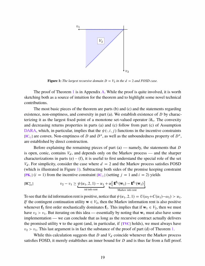
Theorem 1. Fix d > 1 and define the set Vd WD¶

v 2 Ud W vd > vd�1 > � � � > v1

·

.

(a) There exists a largest recursive domainD. It is a non-empty, convex, and open cone in Ud

that satisfies Vd � D. For fixed Markov process, D is independent of the discount factor

˛ 2 .0; 1/ and the utility function U.�/.36

(b) The constraint correspondence � W D ! .U�D/d is nonempty-valued and has a convex

graph.

(c) D� � D is nonempty, convex, has decreasing returns (ie, if v 2 D, then av 2 D for all

a 2 .0; 1�), and is unbounded below (ie, for all k < 0 there exists some v 2 D such that

v � k1).

(d) If the Markov process satisfies FOSD, then D� � Vd .

(e) If the Markov process satisfies either MLRP or PPR, then D D Vd .

(f) If the Markov process satisfies either MLRP or PPR and, in addition, the agent has CARA

utility, then D D Vd D D�.

(35) Different recursive formulations yield different domains. For example, while the domain in Fernandes and

Phelan (2000) is (necessarily) isomorphic to ours, it is defined contingent on the previous period’s report.

That is, their domain is actually a functionW W S ! 2Ud

, and the collection of sets fW.s/gs2S must be solved

for jointly. Consider the case where d D 2 and the Markov process satisfies MLRP. By part (e) of Theorem

1, our domain is the set V2, which is independent of the transition probabilities (within the MLRP class).

For a given v 2 V2 and s 2 S , let vp.s/ WD Efs Œv� denote the ex ante promised utility, and v�.s/ WD Ef3�s Œv�

denote the threat point utility, the utility the agent gets if he lied in the last period about his type. For each

s 2 S , the setW.s/ consists of tuples of the form .vp.s/; v�.s//. It is easy to see thatW.1/ D�

f11 f12

f21 f22

�

V and

W.2/ D�

f21 f22

f11 f12

�

V , which exhibits the isomorphism. Thus, W.1/ and W.2/ are cones and are symmetric

about the diagonal in R2��. Importantly, the sets W.s/ depend on the transition probabilities (even within the

MLRP class). For example, if types are iid, then W.1/ D W.2/ D f.t; t/ W t < 0g, while with positive serial

correlation, they are disjoint open cones.

(36) That is, it is independent of the utility function within the class allowed for by Assumption DARA.

18

v2

v1

V2

Figure 1: The largest recursive domain D D V2 in the d D 2 and FOSD case.

The proof of Theorem 1 is in Appendix A. While the proof is quite involved, it is worth

sketching both as a source of intuition for the theorem and to highlight some novel technical

contributions.

The most basic pieces of the theorem are parts (b) and (c) and the statements regarding

existence, non-emptiness, and convexity in part (a). We establish existence of D by charac-

terizing it as the largest fixed point of a monotone set-valued operator Bı. The convexity

and decreasing returns properties in parts (a) and (c) follow from part (c) of Assumption

DARA, which, in particular, implies that the .�; i; j / functions in the incentive constraints

[ICij ] are convex. Non-emptiness of D and D�, as well as the unboundedness property of D�,

are established by direct construction.

Before explaining the remaining pieces of part (a) — namely, the statements that D

is open, conic, contains Vd , and depends only on the Markov process — and the sharper

characterizations in parts (e) – (f), it is useful to first understand the special role of the set

Vd . For simplicity, consider the case where d D 2 and the Markov process satisfies FOSD

(which is illustrated in Figure 1). Subtracting both sides of the promise keeping constraint

[PKi ] (i D 1) from the incentive constraint [ICij ] (setting j D 1 and i D 2) yields

v2 � v1 � .u1; 2; 1/ � u1

iid info rent

C˛�

Ef2.w1/ � Ef1.w1/�

Markov info rent

[IC�21]

To see that the iid information rent is positive, notice that .u1; 2; 1/ D U.!2CC.u1/�!1/ > u1.

If the contingent continuation utility w 2 V2, then the Markov information rent is also positive

whenever f2 first order stochastically dominates f1. This implies that if w1 2 V2, then we must

have v2 > v1. But iterating on this idea — essentially by noting that w1 must also have some

implementation — we can conclude that as long as the recursive contract actually delivers

the promised utility v to the agent (and, in particular, if [TVC] holds), we must always have

v2 > v1. This last argument is in fact the substance of the proof of part (d) of Theorem 1.

While this calculation suggests that D and Vd coincide whenever the Markov process

satisfies FOSD, it merely establishes an inner bound for D and is thus far from a full proof.

19

Even with CARA utility, while it is easy to see that D must be a cone, it is not clear which

cone it equals.37 Indeed, even in the CARA case, it is perhaps unexpected that the domain

would equal a set, such as Vd , that is independent of both the transition probabilities fi and the

endowment sizes !i . With general preferences satisfying Assumption DARA, it is not even

clear that D should be a cone.38

The remainder of the proof fills in these gaps by studying more detailed properties of

the operator Bı. This requires several steps. In the first step, we show, by direct calculation,

that (i) Vd � Bı.Vd / for general Markov processes and (ii) Vd is a fixed point of Bı when

the Markov process satisfies FOSD. Point (i) implies that Vd � D always; when FOSD fails,

the inclusion is typically strict because the iid and Markov information rents act in “opposite

directions.”39 When the Markov process satisfies FOSD, these sources of information rents

act in the same direction, but point (ii) still leaves open the question whether Vd is the largest

fixed point of Bı.

In the second step — which is the most novel and perhaps most involved part of the

proof — we focus on the case of CARA utility and show that Vd is indeed the largest fixed

point of Bı in two special cases with positive serial correlation. While the operator approach

itself is not new,40 we show how to construct Bı and its iterates in closed form when the

Markov process satisfies either MLRP or PPR. To do this, we formulate and solve an auxiliary

linear programming problem that characterizes exactly the set of implementable v when the

wi are required to satisfy an appropriate set of linear constraints. Under MLRP or PPR, we can

determine which constraints in the linear program bind at the optimum, and thus determine

its solutions. By iterating this procedure, we obtain better and better outer approximations

of the domain D and can verify that no convex cone strictly larger than Vd can constitute a

largest fixed point of Bı. Thus, D D Vd under CARA utility and MLRP or PPR. We show

that D� D Vd in these cases as well by explicitly constructing a feasible recursive contract that

(37) The recursive constraints are always linear in contingent continuation utilities wi . The absence of wealth

effects in the CARA case implies that the functions, and hence the constraints, are also linear in the flow

utilities ui .

(38) The DARA property, part (c) of Assumption DARA, implies rather directly that D must have decreasing

returns in the sense of part (c) of Theorem 1. But it is not clear that D should have “constant returns,” as

required if it is conic.

(39) For example, when d D 2 the Markov information rent in [IC�21] may be written as ˛.f22�f12/�.w12�w11/. If

FOSD is not satisfied (ie, if f22 �f12 � f11 �f21 < 0), any w1 2 V2 will confer negative Markov information

rents. Intuitively, negative serial correlation relaxes the incentive constraints because it implies that private

information is short-lived (relative to the iid benchmark). Following the same linear programming procedure

used in Appendix A.2.2, the reader may easily verify in this case thatD D¶

v 2 R2�� W v2 > .f21=f11/v1

·

)

V2.

(40) It dates back to at least Abreu, Pearce and Stacchetti (1990) in the context of repeated games, and was used

in Fernandes and Phelan (2000) to establish an existence result analogous to the existence statement in part

(a) of Theorem 1. One non-standard aspect of our environment, relative to those papers, is that the range of

flow utilities U is both unbounded and open. This makes establishing even basic properties of D somewhat

subtle, and effectively requires transfinite iterations of the Bı operator.

20

“stops” after finitely-many steps, and is therefore guaranteed to satisfy [TVC].41

The final step extends these ideas to general utility functions and type processes. The

essential idea is to characterize iterates of Bı via solutions of auxiliary concave (instead

of linear) programming problems. The solutions to these concave programs are, perhaps

surprisingly, independent of all model primitives aside from the transition probabilities. Thus,

in particular, all properties of D established in the much simpler CARA case — namely,

the cone property and the fact that D D Vd under PPR/MLRP — immediately extend to

general utilities. Moreover, solutions to these programs — which correspond to points in the

boundary of D — require that the flow utility terms ui D 0. Thus, the boundary points cannot

be implemented, and D must be open. To see an example of this, consider again the d D 2 and

FOSD case. Let v lie in the lower boundary of D D V2, so that v2 D v1. Because the Markov

information rent is positive under FOSD, [IC�21] implies that any menu implementing v must

satisfy u1 D 0. This is impossible — it requires the low endowment type to receive infinite

consumption — and so v in this lower boundary cannot be implemented.

4.3. Regularity Conditions

Having characterized implementable contracts, the rest of the analysis focuses on characterizing

optimal contracts. To ensure that the optimization problem in the recursive problem [RP] is suf-

ficiently well-behaved, we require that the environment satisfy a few mild regularity conditions.

Our approach here is to state a small set of conditions directly in terms of derived objects, and

which can be readily verified on a case-by-case basis for particular parameterizations.

Definition 4.1. The environment is regular if Conditions R.1–R.3, stated below, all hold. The

environment is [TVC]-regular if it is regular and, in addition, satisfies Condition R.4.

R.1 (Finite Value) The value function for [RP], P , is well-defined and real-valued on D � S .

R.2 (Value Continuity) For any v 2 D and recursive contract � 2 „.v/, the first-best value

function Q� satisfies

lim inft!1

˛t

�

infh2H

Q��

v.t/.h/; s.t/.h/�

�

� 0

R.3 (Constraint Qualification) Let �ı.v/ � �.v/ denote the set of all menus that are feasible

at v and, in addition, satisfy all of the incentive compatibility constraints [ICij ] (i > j ) as

strict inequalities. For each v 2 D, �ı.v/ ¤ ∅.

(41) We conjecture that D D D� D Vd for any utility function satisfying Assumption DARA when the Markov

process satisfies the weaker FOSD condition. Extending part (e) of the theorem (ie, the equality D D Vd ) is

complicated because we are unable to determine, in general, which constraints in the auxiliary LP bind at

the optimum. Extending the explicit construction behind part (f) of the theorem (ie, the equality D� D Vd )

poses no conceptual challenge but is extremely tedious.

21

R.4 ([TVC] Existence) There exists a recursively optimal contract �� 2 „�.v.0//.42

Conditions R.1–R.3 are mild technical conditions that allow us to establish basic prop-

erties of the principal’s recursive problem [RP]. For example, Condition R.2 and the well-

posedness criterion in Condition R.1 automatically hold when the consumption domain C is

bounded below, as is the case when the agent has CRRA utility. In general, both Conditions

R.1 and R.2 can be verified by constructing real-valued functions that serve as upper and

lower bounds for P and checking that the flow cost function C.�/ satisfies appropriate growth

conditions. We show how to carry out these verification steps for CARA utility in the appendix;

the most involved step is constructing a real-valued function to serve as an upper bound for

P .43 Condition R.3 is a standard sufficient condition for the existence of Lagrange multipliers,

thereby allowing us to use Lagrangian methods, and is guaranteed to hold when the transition

probabilities ffigi2S are FOSD-ordered or affinely independent. Notably, affine independence is,

in a particular sense, without loss of generality.44 The following lemma records this discussion.

Lemma 4.2. The regularity conditions can be verified in the following cases:

(a) Condition R.3 holds if either (i) the Markov process satisfies FOSD, or (ii) the transition

probabilities ffigi2S are affinely independent.

(b) If the agent has CARA utility and the Markov process satisfies MLRP or PPR, the envir-

onment is regular.

The proof of Lemma 4.2 is in Supplementary Appendix S.3.1.

Condition R.4, on the other hand, is a somewhat more substantive requirement and is

important for the proofs of our main economic results, Theorems 3 and 4. In settings such as

ours where U is not bounded, Condition R.4 typically cannot be verified without solving for

the optimal contract in (nearly) closed form. Even with iid types this can only be done in a

few special cases, and we do not know of any cases with Markovian types where it is possible.

These issues are discussed in more detail in Appendix S.1.3. On the other hand, we do not

(42) v.0/ is the initial condition for the promised utility process. It may be given exogenously, or optimally

initialized as in the efficiency problem [Effi ] described below in Section 5.1.

(43) We use the value function induced by the (suboptimal) [TVC]-implementable contract constructed in the

proof of part (f) of Theorem 1. The main difficulty of that construction is precisely ensuring that the contract

has finite value.

(44) For any given dimension d , transition matrices that fail affine independence (or, equivalently, linear inde-

pendence) are non-generic under any standard genericity notion. Of course, important examples, such as the

iid benchmark, are non-generic in this sense. Even in these cases, affine independence is without loss in the

following sense. But if the affine hull of ffi gi2S has dimension d 0 < d , it is always possible to (i) reduce

the dimensionality of the promised utility state variable to d 0 by “pooling” the promise keeping constraints

together with appropriate weights, and (ii) then analyze recursive contracts on this lower-dimensional domain.

In the extreme case of iid types (d 0 D 1), this reduces to the scalar state variable of, eg, Thomas and Worrall

(1990). The projection onto this lower-dimensional space is linear, and thus preserves convexity, topological,

and smoothness properties of D and P , so the analysis can be carried out essentially verbatim after this

reduction. Details are available upon request.

22

know of any examples in which Condition R.4 fails, either, and in light of Lemma 3.2 it should

be viewed as a minimal consistency requirement on any solution to [RP]. (As noted in footnote

34, Condition R.4 can actually be weakened slightly.)

4.4. Bellman Equation

The main result of this section shows that the principal’s value function P satisfies a standard

Bellman equation, characterize its properties, and establish basic properties of the optimal

contract that it generates.

Theorem 2. Suppose the environment is regular. Then the principal’s value function P W

D � S ! R satisfies the functional equation

P.v; s/ D min.ui ;wi /i2S 2�.v/

X

i2S

fsi

�

C.ui ; i/C ˛P.wi ; i/�

[FE]

and, for each s 2 S , P.�; s/ is convex and continuously differentiable. Moreover:

(a) P is the pointwise smallest solution to [FE] that lies pointwise above Q�, the first-best

value function.

(b) P is strictly increasing in v1 and non-monotone in vi for all i > 1. For any sequence

.vn/ � D such that vn ! bd D, the boundary of D, we have P.vn; s/ ! C1.

(c) There exists a recursively optimal contract �� such that, for each i 2 S , the functions

��f .�; �; i/ and ��c.�; �; i/ depend on .v; s/ only through .vi ; : : : ; vd /.45

(d) The policy correspondence derived from [FE] is nonempty-, compact-, and convex-valued

and is upper hemicontinuous.

(e) If, in addition, the environment is [TVC]-regular, then (i) each P.�; s/ is strictly convex, (ii)

there exists a unique recursively optimal contract ��, which satisfies the independence

properties stated in part (c), (iii) for each s 2 S , ��.�; s/ is a continuous function, and (iv)

the induced allocation Qu�� solves the sequence problem [SP].

The proof of Theorem 2 is in Supplementary Appendix S.3. The proof makes clear

precisely which of the Conditions R.1–R.4 are used to establish each property stated in the

theorem.

While many properties described in Theorem 2 are standard, two points warrant further

explanation. First, part (b) highlights important non-monotonicity and boundary properties

of the value function that derive from fundamental features of the incentive constraints. The

unboundedness ofP near the boundaries ofD follows from the same logic used to establish that

(45) That is ��f .v; s; i/ D ��f .v0; s0; i/ for all .v; s/; .v0; s0/ 2 D�S such that vj D v0j for all j � i , and similarly

for ��c .

23

D is open in part (a) of Theorem 1; indeed, these two properties are essentially equivalent.46

To get intuition for the non-monotonicity properties, consider once again the case in which

d D 2 and the Markov process satisfies FOSD (recall Figure 1). An increase in v1 tightens

both the promise keeping constraint [PKi ] (i D 1) and the incentive constraint [IC�21], leading

to unambiguously higher costs for the principal. An increase in v2, on the other hand, tightens

[PKi ] (i D 2) and adds slack to [IC�21]. The first effect increases costs, while the second effect

lowers costs; depending on the current state .v; s/, either of these effects can dominate. When

v1 � 0 (ie, v is close to the upper boundary of V2), the first effect dominates and P is increasing

in v2. When v is close enough to the diagonal (ie, the lower boundary of V2 ), the second effect

dominates and P is decreasing in v2.

Second, part (c) states that the optimal contract does not depend on all components of

the state variable .v; s/. The independence of the policy functions on the previous report s 2 S

follows directly from the interim nature of the promised utility state variable. Because the

constraint set �.v/ does not depend on s, it is easy to see that the optimization problem in [FE]

may be decomposed into d separate problems, each of which conditions only on the agent’s

current report.47 Thus, v 2 D is a “sufficient statistic” for .v; s/ for the purpose of computing

optimal flow and continuation utilities. Of course, the agent’s previous report s 2 S is essential

for determining the principal’s value at each history, and is thus a necessary component of

the principal’s state variable. The fact that the policy functions for type i 2 S depend on the

current promised utility v only through its components .vi ; viC1; : : : ; vd / is a consequence of

Assumption NHB, which implies that ui and wi only appear in those incentive constraints that

deter deviations by higher types.48

5. The Optimal Contract — Long-Run Properties

We now characterize the long-run properties of the optimal contract. In Section 5.1, we

introduce a martingale that plays a central role in our characterization. Then, in Sections 5.2

and 5.3 we present our main results on, respectively, absolute and relative immiseration.

(46) Because P is unbounded even on bounded sets, we are unable to use standard contraction mapping arguments

to ensure that P is the unique solution to the functional equation [FE]. However, part (a) of Theorem 2 states

that P is the smallest solution in an appropriate class. This fact is essential both for establishing certain

analytical properties of P (eg, that the directional derivative in Proposition 5.1 is non-negative) and for

numerical computation.

(47) See Appendix B.3.3 for more details. We emphasize that this separation is not possible in the Fernandes and

Phelan (2000) approach for reasons described in footnote 35.

(48) Without Assumption NHB, the policy functions ui .�/ and wi .�/ would depend on .v; s/ through the entire

vector of promises v, as these variables must be chosen to deter deviations by both higher and lower types.

24

5.1. The Differential Martingale

In the iid setting, Thomas and Worrall (1990) show that the derivative of their value function

with respect to (scalar) ex ante promised utility is a martingale. The appropriate martingale

in our Markovian setting is a somewhat subtle, but natural, generalization. We denote the

derivative of P at .v; s/ by DP.v; s/ D .P1.v; s/; : : : ; Pd .v; s//, where Pi.v; s/ is the partial

derivative with respect to the component vi . Denote the directional derivative of P.�; s/ in

direction 1 D .1; : : : ; 1/ 2 Rd by D1P.v; s/ WD lim"#0 ŒP.v C "1; s/ � P.v; s/� =".

Proposition 5.1. Suppose that the environment is regular. Then the stochastic process induced

by the optimal contract,�

D1P.v.t/; s.t//

�1

tD0, is a non-negative martingale. If the environment

is [TVC]-regular, then this process is strictly positive.

The proof of Proposition 5.1 is in Appendix B. We will refer to this stochastic process as

the differential martingale. The statement of the proposition includes three important pieces:

the martingale property, the direction 1 in which the directional derivative is taken, and the

fact that the directional derivative is strictly positive.

The intuition for the martingale property is simply that the principal optimally smooths

costs over time and across states. To be a bit more precise, fix a vector v 2 D and consider

the cost to the principal of increasing this promise to v0 WD v C "1 for some " > 0. When

" > 0 is small, this cost of this increase in promises is close to the marginal cost D1P.v; s/.

One way to deliver the additional utility in an incentive-compatible way is to increase each of

the continuation promises wi to w0i WD wi C ."=˛/1. To a first-order approximation, the cost

of this perturbation isPd

iD1 fsiD1P.wi ; i/. An envelope theorem argument implies that this

perturbation is locally optimal, implying that the marginal costs are equal, giving us precisely

the martingale property

D1P.v; s/ D

dX

iD1

fsiD1P.wi ; i/

in Proposition 5.1.

To understand why the directional derivative must be taken in the direction 1, notice that

this is the unique direction of change for v that increases the agent’s ex ante continuation utility

while leaving his information rent unchanged. As in Section 4.2, substituting the promise

keeping constraint [PKi ] (i D j ) into the incentive constraint [ICij ] (i > j ) gives an alternative

way to write the latter:

[IC�ij ] vi � vj � .uj ; i; j / � uj C ˛

�

Efi�

wj

�

� Efj�

wj

��

Written this way, it is clear that a perturbation of v leaves the left-hand side of the [IC�ij ]

constraints unchanged if, and only if, it is taken in the direction 1. Another way to see this

is by considering perturbations of the wi . Suppose the principal wants to change wi to Owi in

such a way that the expected value to type i is " > 0, ie, Efi�

Owi

�

� Efi Œwi � D ". In general,

25

each type values such a perturbation differently, as each (current) type has distinct beliefs

concerning future types. By setting Owi � wi D "1, the principal guarantees that all types value

this perturbation in the same way, ie, that Efj�

Owi � wi

�

D " for all j 2 S . (When the transition

probabilities ffigdiD1 are affinely independent, 1 is the unique direction with this property.)

Finally, the intuition for strict positivity of the directional derivative D1P.v; s/ is similar.

As we have seen in part (b) of Theorem 2, there are typically regions of the domain on which

the value function is decreasing in certain directions, so it is not true that arbitrary directional

derivatives are non-negative. The value function is decreasing or non-monotone in certain

directions because increasing a single component of v has two effects. First, it increases the

promise to some type, which mechanically increases costs. Second, it either adds slack to or

tightens certain incentive constraints [IC�ij ]. Whenever it adds “enough” slack to the incentive

constraints, the second effect dominates and leads to an overall decrease in costs. The above

arguments show that, by taking the derivative in direction 1, the second effect completely

washes out, leaving only the mechanical increase in costs due to higher promised utilities.

E�iciency and the TW Martingale: At this point, it is useful to make two related obser-

vations that are useful going forward. First, Markovian private information induces a novel

intertemporal distortion that is not present with iid types. Second, when the type process is

iid, the differential martingale reduces to the martingale from Thomas and Worrall (1990)

(henceforth, the TW martingale).

To see how this is so, consider the question, What is the cost-minimizing way for the

principal to give a type i agent at least ex ante promised utility v 2 U, without consideration

of today’s incentives? Formally, this is equivalent to solving the problem49

K.w; i/ WD minwi 2D

P.wi ; i/

s.t. Efi Œwi � � w[Effi ]

We say that solutions to the problems [Effi ] are efficient. Very informally, efficiency corresponds

to a kind of “renegotiation-proofness”: even after the agent reveals himself to be of type i and

so incentive compatibility in the current period is no longer a concern, there is no way for the

principal to reduce her costs while leaving the agent at least as well off, in expectation, going

forward.

In general, the optimal contract is typically not efficient, as the principal must keep in

mind that her choice of wj affects the Markov information rent in each [IC�ij ] with i > j .

However, the optimal contract is efficient after reports of !d , ie, for all .v; s/ 2 D the policy

function wd .v; s/ solves [Effi ] (i D d ) for some optimally-chosen w 2 U. This is because,

under Assumption NHB, the variables ud and wd do not enter into any of the [ICij ], only the

promise keeping constraint [PKi ] (i D d ).

(49) The efficiency problem [Effi ] is analogous to what Fernandes and Phelan (2000) call the “planner’s problem,”

while our recursive problem [RP] is analogous to what they call the “auxiliary planner’s problem.”

26

When types are iid, the optimal contract is efficient at all histories. To see this, note that

in the iid case, the Markov information rent in [IC�ij ] vanishes. Therefore, the continuation

utility vectors wi enter the constraints of [FE] (with each [IC�ij ] taking the place of [ICij ])

only through the promise keeping constraints [PKi ]; there, they appear only through their

expectations E� Œwi �, where � 2 �.S/ is the common vector of transition probabilities. Thus,

optimality clearly implies that, for all .v; s/ 2 D � S and i 2 S , the policy function wi.v; s/

must solve [Effi ] (with fi D � for each i 2 S).

Therefore, along the path induced by the optimal contract, the principal’s value process

is given by K.v.t/; s.t// D P.v.t/; s.t//, where v WD E� Œv�. Thus, ignoring the (in this case)

irrelevant s.t/ argument, K is the value function of Thomas and Worrall (1990) and the process�

K 0.v.t/; s.t//�1

tD0is the TW martingale. It is easy to see from the envelope and first-order

conditions for [Effi ] (any i 2 S) that K 0.w; i/ D Pj .wi ; i/=�j and, thus, summing over j 2 S ,

thatK 0.v; s/ D D1P.v; s/. Hence, our differential martingale coincides with the TW martingale

when types are iid. This is not to say that K.v; s/ D P.v; s/ or K 0.v; s/ D D1P.v; s/ for all

v 2 D, as there are many points v 2 D that could not possibly be efficient.50 These objects

need only coincide at the optimum.

However, the differential and TW martingales are not equivalent. As we show by example

in Section 7.3 (where we consider CARA utility and type processes that satisfy MLRP), in the

iid setting the TW martingale can be derived via perturbations that are not incentive compatible

when types are persistent. Thus, while there are other directional derivative processes that

define martingales when types are iid, only the directional derivative D1P.v; s/ is guaranteed

to define a martingale for more general type processes.

5.2. Absolute Immiseration

With the differential martingale in hand, we may state our first main economic result. We refer

to it as Absolute Immiseration because it states that the level of the agent’s (promised) utility,

and thus consumption, tends to its lower bound — ie, the agent becomes impoverished in

absolute terms.

Theorem 3 (Absolute Immiseration). Suppose the environment is [TVC]-regular. Under the

optimal contract:

(a) D1P�

v.t/; s.t/�

! 0 almost surely.

(b) v.t/i ! �1 almost surely for all i 2 S .

(c) u.t/i ! �1 and c

.t/i C !i ! c in probability for all i 2 S .

(50) The first-order conditions in [Effi ] imply that all of the partial derivatives Pj .wi ; i/ are positive; this is true

even when fi in [Effi ] is replaced with some arbitrary “prior” q 2 �.S/. But as we have seen in part (b) of

Theorem 2, P.�; s/ is non-monotone in all components of v aside from v1. Thus, there are regions of D on

which Pj .�; s/ < 0 for all j ¤ d . This is true even in the iid case.

27

(d) If the type process satisfies UPR, then the convergence in part (c) can be strengthened

from “in probability” to “almost surely.”

Thus, neither flow utility nor promised utility possesses a stationary distribution under the

optimal contract. Net consumption possesses a stationary distribution if and only if c > 0, in

which case it puts full mass at the lower bound c.

The proof of Theorem 3 is in Appendix B.4. We note that even the restriction to UPR

type processes in part (d) nests the cases of (i) iid types for any d and (ii) any Markovian type

process when d D 2. These two cases alone include essentially all extant immiseration-type

results in the literature.51 While the general case covered by part (c) is stated in terms of a

weaker mode of convergence (for technical reasons described below), we emphasize that this

is still sufficient to rule out any stationary distribution for net consumption other than the Dirac

measure at the lower bound c. Thus, we conclude that Absolute Immiseration is very robust.

The intuition, familiar from Thomas and Worrall (1990),52 is that, due to risk aversion,

providing incentives is cheaper for the principal when promised utility is lower. In particular,

the principal provides truth-telling incentives by making (flow and continuation) utility vary

depending on the reported type. Suppose, for instance, that d D 2 and the principal wants to

induce a spread of " > 0 between the flow utility for types 2 and 1, ie, u2 � u1 D ". When the

previous report was s 2 S and " > 0 is small, this costs the principal approximately

fs1C.u1; 1/C fs2C.u1; 2/

level

C " � fs2C0.u1; 2/

variability

Thus, because C.�; 2/ is convex, the cost of making utility variable is an increasing function of

the utility level. In the long run, it is optimal for the principal to drive this cost of incentive

provision to zero by forcing the level of the agent’s utility as low as possible.

To better understand each part of Theorem 3, it is useful to walk through a sketch of the

proof. While the basic idea of using the Martingale Convergence Theorem is familiar from

Thomas and Worrall (1990), the details of the argument are significantly more subtle when

types are not iid, and is important to understand why.

The proof of part (a) is based three simple ideas. First, the principal optimally smooths

costs over time and across states, as captured by the differential martingale from Proposition

5.1. Second, the first-best contract is not implementable when the agent has private information.

While this is easy to see, the key is to translate this fact into a statement about splitting of the

differential martingale. In particular, we show that whenever the state is of the form .v; d /where

v D �c.v0; s; d/ for some v0 2 D — ie, given some initial condition, the optimal contract maps

to v after a d report — it must be that D1P.v; d / ¤ D1P.wi ; i/ for some i 2 S . That is, whenever

(51) The one exception we are aware of is the example in Williams (2011) in which the hidden endowment

follows a Brownian motion with drift. We provide a detailed comparison in Section 6.2.

(52) Golosov, Kocherlakota and Tsyvinski (2003) provide an especially clear discussion in the related context of

“separable” taxation models (but see Section 7 for some important differences between their setup and ours).

28

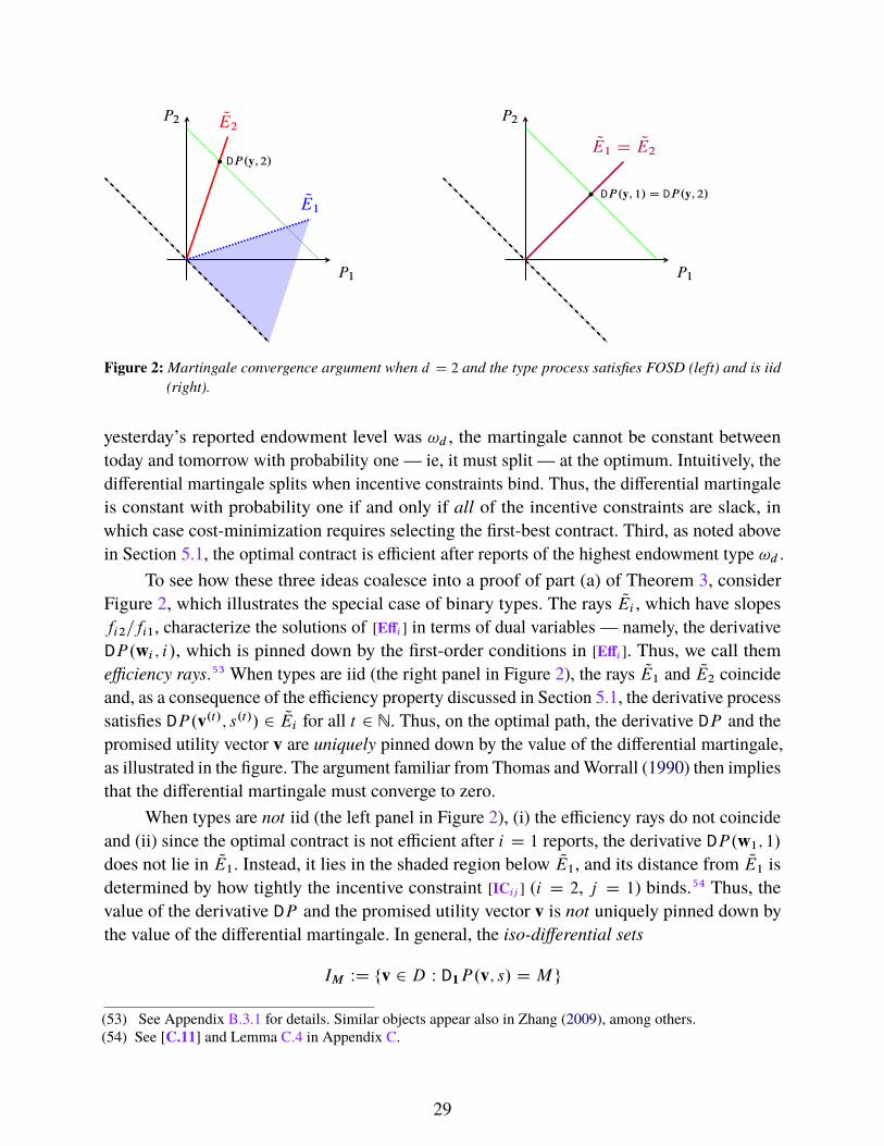
P1

P2 QE2

QE1

DP.y; 2/

P1

P2

QE1 D QE2

DP.y; 1/ D DP.y; 2/

Figure 2: Martingale convergence argument when d D 2 and the type process satisfies FOSD (left) and is iid

(right).

yesterday’s reported endowment level was !d , the martingale cannot be constant between

today and tomorrow with probability one — ie, it must split — at the optimum. Intuitively, the

differential martingale splits when incentive constraints bind. Thus, the differential martingale

is constant with probability one if and only if all of the incentive constraints are slack, in

which case cost-minimization requires selecting the first-best contract. Third, as noted above

in Section 5.1, the optimal contract is efficient after reports of the highest endowment type !d .

To see how these three ideas coalesce into a proof of part (a) of Theorem 3, consider

Figure 2, which illustrates the special case of binary types. The rays QEi , which have slopes

fi2=fi1, characterize the solutions of [Effi ] in terms of dual variables — namely, the derivative

DP.wi ; i/, which is pinned down by the first-order conditions in [Effi ]. Thus, we call them

efficiency rays.53 When types are iid (the right panel in Figure 2), the rays QE1 and QE2 coincide

and, as a consequence of the efficiency property discussed in Section 5.1, the derivative process

satisfies DP.v.t/; s.t// 2 QEi for all t 2 N. Thus, on the optimal path, the derivative DP and the

promised utility vector v are uniquely pinned down by the value of the differential martingale,

as illustrated in the figure. The argument familiar from Thomas and Worrall (1990) then implies

that the differential martingale must converge to zero.

When types are not iid (the left panel in Figure 2), (i) the efficiency rays do not coincide

and (ii) since the optimal contract is not efficient after i D 1 reports, the derivative DP.w1; 1/

does not lie in QE1. Instead, it lies in the shaded region below QE1, and its distance from QE1 is

determined by how tightly the incentive constraint [ICij ] (i D 2, j D 1) binds.54 Thus, the

value of the derivative DP and the promised utility vector v is not uniquely pinned down by

the value of the differential martingale. In general, the iso-differential sets

IM WD fv 2 D W D1P.v; s/ D M g

(53) See Appendix B.3.1 for details. Similar objects appear also in Zhang (2009), among others.

(54) See [C.11] and Lemma C.4 in Appendix C.

29

forM > 0 are surfaces inD and, even on the optimal path, it is possible that .v.t// travels along

such a surface. Thus, convergence of the differential martingale does not directly imply that

the derivative or promised utility processes converge. We emphasize that this is not merely a

mathematical complication. Rather, it is a fundamental consequence of incentive compatibility

in the presence of persistent private information.

We overcome these difficulties by observing that the derivative process satisfies a kind

of “renewal” property: though it takes excursions away from the efficiency rays during strings

of consecutive low-type reports, it returns to the ray QE2 after the first high-type report, and

then the cycle starts again. We thus look along the subsequence of dates at which s.t/ D 2.

(Part of the following argument is illustrated in the left-hand panel of Figure 2.) Fix some

path and denote this (deterministic) subsequence of dates by .� t/1tD0. By the Martingale

Convergence Theorem, unless the chosen path is non-generic, the differential martingale must

converge to some finite, non-negative number along this path. If the limit is some number

C > 0, then since DP.v.� t /; s.� t // 2 QE2 for all t 2 N, it must be that v.� t / ! y 2 D with

DP.y; 2/ 2 QE2 and D1P.y; 2/ D C . Because every state in the Markov process for endowments

is recurrent, unless the chosen path is non-generic it features s.� t C1/ D 1 for infinitely many

t and s.� t C1/ D 2 for infinitely many t . Because the differential martingale converges along

the entire sequence, and by continuity of the policy functions and directional derivative, it

follows that D1P.y; 2/ D D1P.��.y; 2; 1/; 1/ D D1P.�

�.y; 2; 2/; 2/ D C . But we have argued

above that this is not possible, as it implies that the first-best is implementable. Thus, the limit

of the differential martingale must be zero, completing the proof sketch of part (a).

The remainder of the proof, which establishes parts (b)–(d) of Theorem 3, works to

connect convergence properties of the differential martingale to convergence properties of

flow and promised utilities. Again, this exercise is substantially complicated by the fact that

the iso-differential sets are surfaces in D. The proof is fairly involved, but the main idea is

to show that convergence of the differential martingale to zero implies convergence of the

vector of Lagrange multipliers to the zero vector. When the type process satisfies UPR (which,

recall, automatically holds in the d D 2 example above), we are able to show that, roughly

speaking, the rate of convergence of the multipliers can be controlled uniformly by the rate of

convergence of the differential martingale. This turns out to be enough to reach the desired

conclusion. The general case, covered by part (c) of Theorem 3, is much more subtle, and we are

unable to establish strong enough uniformity properties to guarantee almost sure convergence

of the multipliers. Instead, we show how to use probabilistic arguments, and the “renewal”

reasoning described above, to establish convergence in probability. Roughly speaking, while

we cannot rule out that the vector of multipliers take infinitely-many excursions away from

the zero vector on any given path, under Assumption Markov the type process mixes quickly

enough to guarantee that such excursions are very rare.55

(55) We are only aware of one other paper in the dynamic contracting literature — namely, Garrett, Pavan and

Toikka (2018) — that establishes results concerning convergence in probability, as opposed to almost sure

convergence, of the optimal contract. By design, their “variational approach” cannot in principle establish

30

5.3. Relative Immiseration

Imagine two agents, A and B , who have received the same sequence of realized endowments

up through period t � 1. In period t , agent A receives a higher endowment than agent B.

How much better off is A than B going forward, as measured by the difference between their

continuation utilities? Our second main economic result shows that, as t increases, the impact

on continuation utilities of this last report grows without bound. We refer to it as Relative

Immiseration because it states that the difference in promised utilities across different types of

agents grows — ie, low endowment types become impoverished relative to high endowment

types.

Theorem 4 (Relative Immiseration). Suppose the environment is [TVC]-regular and the Markov

process satisfies FOSD. Under the optimal contract:

(a) v.t/i � v

.t/i�1 ! C1 in probability for all i D 2; : : : ; d . Moreover, for all t 2 N,

Var�

v.tCk�1/

s.tCk/

ˇ

ˇ

ˇv.t/; s.t/

�

! C1 as k ! 1

in probability.

(b) If, in addition, Absolute Immiseration occurs almost surely (namely, u.t/i ! �1 almost

surely for each i 2 S), then the convergence in part (a) can be strengthened from “in

probability” to “almost surely.” Moreover, in this case

Var�

v.t/

s.tC1/

ˇ

ˇ

ˇv.t/; s.t/

�

! C1 as t ! 1

almost surely. In particular, these conclusions hold if the Markov process satisfies PPR.

The proof of Theorem 4 is in Appendix B.5. Mathematically, Relative Immiseration is

a consequence of Absolute Immiseration. In particular, the incentive constraint [IC�ij ] with

j D i � 1 is

vi � vi�1 � .ui�1; i; i � 1/ � ui�1 C ˛�

Efi Œwi�1� � Efi�1 Œwi�1�

�

When the type process satisfies FOSD, Proposition 1 implies that the Markov information rent

term is non-negative, and parts (c) and (d) of Theorem 3 imply that the iid information rent term,

which is always non-negative, grows without bound (either in probability or almost surely).

It follows from the above incentive constraint that the difference vi � vi�1 must also grow

without bound. The proof formalizes this argument, and establishes the statements regarding

conditional variances as easy corollaries.

pathwise properties of the optimal contract. Thus, their results are fundamentally different from part (c) of

Theorem 3, which is stated in terms of convergence in probability only due to our technical limitations. The

proof of part (c) actually involves establishing quite strong pathwise properties of the optimal contract, and

we conjecture that the result can be strengthened from convergence “in probability” to “almost surely.”

31

While Absolute Immiseration in Theorem 3 is driven by the fact lower levels of promised

utility make it cheaper for the principal to provide incentives through variability of (flow and

promised) utility, this does not tell us how variable utility is in the limit. Relative Immiseration

in Theorem 4 states that, as the cost of incentive provision decreases to zero, the variability of

promised utility increases without bound. Intuitively, the principal does not waste the ability

to provide high-powered incentives as they become affordable. This observation, while simple,

has important implications for long-run inequality under the optimal contract.

In particular, Relative Immiseration formalizes the idea that “pathwise inequality” in-

creases over time, and without bound, under the optimal contract. Any given sequence of

types up through date t � 1 is summarized by a state variable .v.t/; s.t//. At the beginning of

period t , before the current endowment shock !s.tC1/ is realized, the agent’s type-contingent

continuation utility v.t/

s.tC1/ is a random variable with conditional mean

[5.1] Eh

v.t/

s.tC1/

ˇ

ˇ

ˇv.t/; s.t/

i

D

dX

iD1

fs.t/;iv.t/i

and conditional variance

[5.2] Var�

v.t/

s.tC1/

ˇ

ˇv.t/; s.t/�

D

dX

iD1

fs.t/;i

�

v.t/i � E

h

v.t/i

ˇ

ˇ

ˇv.t/; s.t/

i�2

The conditional mean is just the “ex ante” promised utility at date t (as in Thomas and Worrall

(1990)), and Theorem 3 shows that it decreases without bound on the optimal path. Under the

first-best (recall Section 4.1), the conditional variance is always zero because consumption is

perfectly stabilized. The first half of part (b) of Theorem 4 states that, in the second-best and

under FOSD, the function i 7! v.t/i is (i) is strictly increasing and (ii) becomes arbitrarily steep

in the long run. Thus, idiosyncratic and transient shocks — namely, the realized endowment in

period t — translate to large, permanent differences in welfare. As a consequence, the second

half of part (b) of Theorem 4 says that the conditional variance in [5.2] becomes arbitrarily

large in the long run. Thus, the agent’s uncertainty about his future prospects, before observing

his realized endowment in a given period, increases without bound.

Thus, Relative Immiseration represents one sense in which private information leads

to a severe breakdown of insurance in the long run. But variability of contingent promised

utility is not the only measure of insurance quality, and Theorem 4 does not imply that either

(i) the differences in net consumption .c.t/iC1 C !iC1/ � .c

.t/i C !i/ or (ii) any of the “wedges”

used to quantify allocative distortions (see Section 7) diverge. Indeed, neither is true. When

the consumption domain is bounded below, parts (c) and (d) of Theorem 3 imply that net

consumption converges to the lower bound c. Thus, at the limit, net consumption is completely

stable, always at its lower bound, and the difference between consumption transfers is bounded

— in particular, jc�iC1 � c�

i j D j!iC1 �!i j. In Section 7, we study the dynamics of the insurance

and intertemporal wedges, which are standard measures of departures from the first-best

32

allocation. When the agent has CARA utility, the wedges are “scale invariant” and exhibit

a strong form of mean reversion. Indeed, as we have argued above, Absolute and Relative

Immiseration are driven by the fact that, to minimize costs, the principal aims to provide

maximal incentives with minimal variability of consumption itself.56 Crucially, the facts that

the utility function is (i) concave and (ii) unbounded below imply that small variations in net

consumption lead to very large variations in flow utility when the level of consumption is low.

Thus, Theorem 4 shows that, even as net consumption converges to the constant c, it retains

enough noise to make the variance of utility explode.

We note that, while the statements about conditional variances in Theorem 4 look su-

perficially similar to existing results in the literature, they differ in important ways. A central

finding of Atkeson and Lucas (1992) is that the unconditional (ie, from the t D 0 perspective)

variance of ex ante promised utility (as in [5.1]) grows without bound.57 In an exact analogue

of our model with CARA utility and endowment shocks that are driven by a Brownian motion

with drift, Williams (2011) shows that the distribution of ex ante promised utility spreads out

over time, as the unconditional variance of the Brownian motion naturally tends to infinity.

Both of these results essentially say that a society’s cross-sectional inequality is expected to

grow over time. Importantly, in both papers, promised utility fans out over time due to the

cumulative effect of all previous shocks; in Williams (2011), this follows fairly mechanically

from the fact that the private information process itself has unbounded unconditional variance.

Moreover, both results concern ex ante promised utility — not promised utility contingent on

type. In contrast, Theorem 4 — namely, the stronger statement in part (b) — says that, along

(almost) every path, the impact on inequality of an incremental piece of private information

increases without bound. To capture the notion of an incremental piece of private information,

it is essential that Theorem 4 is stated in terms of promised utilities contingent on type.58

6. Discussion: Robustness of Immiseration

6.1. Revisiting Basic Assumptions

While the baseline model laid out in Section 2 is fairly general, our analysis does rely on three

types of assumptions (enumerated below). Given the fundamental nature of the questions we

consider, it is important to understand the role that each plays in obtaining our results.

(56) Kocherlakota (2010, p. 70) argues that this is the general principle underlying all immiseration-type results.

The general “front-loading principle” emphasized by Albanesi and Armenter (2012) is also related.

(57) To be precise, this is true when utility is logarithmic. In the other cases they consider, the variance of

appropriate functions of promised utility explodes.

(58) This is one conceptual advantage of using interim variables, as opposed to ex ante variables as in Fernandes

and Phelan (2000) or even Thomas and Worrall (1990).

33

Preferences and Source of Private Information: We have focused on the case in which

the agent’s private information concerns his endowment, but this is not essential. Here, we

mention a few other cases of particular interest.

Multiplicative taste shocks: The agent’s utility function over consumption c is U.c; �/ D

�u.c/, where � denotes a subjective taste parameter. The principal minimizes the cost of

providing consumption to the agent. This specification is adopted in many papers starting with

Atkeson and Lucas (1992). When the range of u.�/ is open, bounded above, and unbounded

below, this class of models is essentially identical to our hidden endowment model with CARA

utility.

Productivity shocks with separable preferences: The agent’s utility function over con-

sumption c and labor ` is U.c; `; �/ D u.c/ � v.`; �/, where � is a productivity parameter.

The principal provides consumption to the agent but collects his output �`, and thus aims to

minimize the present discounted value of consumption minus output, c� �`. This specification

is the workhorse of the optimal dynamic taxation literature — see, eg, Golosov, Kocherlakota

and Tsyvinski (2003), Albanesi and Sleet (2006), Zhang (2009), and Farhi and Werning (2013)

for recent contributions, and Kocherlakota (2010) for a survey.

Productivity shocks with non-separable preferences: The agent’s utility function over

consumption c and labor ` is U.c; `; �/, where � is a productivity parameter. The principal’s

objective is the same as above. This clearly generalizes the separable specification described

above, and is studied in, eg, Farhi and Werning (2013) and Golosov, Troshkin and Tsyvinski

(2016).

In each case, it is straightforward to formulate the contracting problem recursively as in

Sections 3 and 4. Under “appropriate technical conditions,” it is also straightforward to extend

parts (a), (c), and (d) of Theorem 3 by following the same proof steps almost verbatim.59 The

proof of part (b), as written, does use the fact that the utility function U.�/ is bounded above,

but it can easily be extended if the flow utility process satisfies weaker uniform integrability

conditions. This is a primary virtue of the martingale approach, which isolates the driving

forces and does not hinge on irrelevant functional form assumptions or other fine details of the

environment.

Indeed, the “appropriate technical conditions” needed to extend Theorem 3 essentially

consist only of monotonicity, concavity, smoothness, and Inada conditions embedded in part (a)

of Assumption DARA. It is well known that these are nearly necessary conditions for Theorem

3, and in each of the above specifications, appropriate analogues of these conditions must

be adopted for Absolute Immiseration to hold more generally.60 On the other hand, parts (b)

(59) The first-best contracts in these models need not fully stabilize consumption, as is the case with endowment

shocks (see Section 4.1), but they are still not implementable and satisfy appropriate self-generation properties

(see Appendix B.3).

(60) The monotonicity and concavity properties guarantee that the first-best is not implementable, the smoothness

conditions imply smoothness of the principal’s value function, and the Inada conditions are important for

reasons discussed in Phelan (1998).

34

and (c) of Assumption DARA are purely technical (as are the regularity conditions described

in Section 4.3, which we do not mention further). As has been previously noted, part (c) of

Assumption DARA is used to guarantee that the space of feasible contracts is convex, and thus

that (i) there is no gain to using randomized contracts and (ii) first-order optimality conditions

are sufficient. These properties are automatically satisfied in the multiplicative taste shock

specification, and can be similarly assumed in the productivity shock specifications.

The primary role of part (b) of Assumption DARA — in particular, the requirement that

the utility function U.�/ is unbounded below — is to ensure that the range of feasible flow

utilities U is open, and thereby rule out corner solutions. When corner solutions are possible,

the directional derivative process may not define a martingale globally, and additional care

is required. In an example with iid and multiplicative taste shocks, Golosov, Tsyvinski and

Werquin (2016) show (in the proof of their Proposition 6) how to deal with these issues when

UD RC, and thus has a single boundary point. In the Markovian setting, the boundary of the

largest recursive domain D is a surface in Rd (typically with no closed-form description), and

it thus seems unavoidable that one must rely on idiosyncratic arguments adapted to the case at

hand. Of course, if one can show that the optimal contract is always interior (in an appropriate

sense), then our martingale arguments apply directly. We would find it very surprising if such

boundary issues, by themselves, could lead to a failure of Absolute Immiseration.

Importantly, part (b) of Assumption DARA also requires that the utility function is

bounded above. This serves as a technical simplification in a few proofs, but its main role

is in determining the shape of the largest recursive domain D in Theorem 1. If, instead, the

utility function were bounded below and unbounded above, then D would be a cone in the

positive orthant RdC; if it were unbounded both above and below (eg, logarithmic utility), then

D would span the entire space Rd . While these differences are not essential for Absolute

Immiseration, they do have important implications for the robustness of Relative Immiseration.

In particular, Theorem 4 — or, at least, the proof technique we employ — uses the fact that

D� � Vd when the Markov process satisfies FOSD (this is part (d) of Theorem 1). For example,

if instead we considered a model where the utility function was bounded below, then Relative

Immiseration would not occur. Even with our Assumption DARA in place, it is possible that

Relative Immiseration would fail when the Markov process exhibits negative serial correlation,

and thus Markov information rents could be negative. Thus, we conclude that, while Relative

Immiseration holds in the broad class of environments covered by Theorem 4 (and appropriate

analogues in the taste- and productivity-shock specifications), it is sensitive to details of the

type process and utility function in ways that Absolute Immiseration is not.

Markov Process: Assumption Markov plays two substantive roles. The recursive represent-

ation itself (Sections 3 and 4) plainly relies on finiteness of the type space and the Markov

property. Beyond this, the joint assumption of finiteness and full connectedness is mainly for

technical convenience. The existence of a highest endowment type does play a role in the

35

proof of Theorem 3, but finiteness of the type space itself seems less important. We conjecture

that Theorem 3 holds for a larger class of ergodic Markov processes on compact type spaces,

thought it is not clear that such a generalization could add new insights.61 To be sure, Theorems

3 and 4 will not hold if the Markov process has absorbing states, so ergodicity is critical.62

Feasible Reporting Strategies: No Hidden Borrowing (Assumption NHB) is the most sub-

stantive assumption, as it limits the agent’s set of feasible reporting strategies. While we do

not view it as economically very restrictive and believe that Theorems 3 and 4 would hold

without it, the proofs would need to be augmented.63 We justify No Hidden Borrowing on

three main grounds. First, constraints on under-reporting seem to be the relevant concern

empirically — see, eg, Feldman and Slemrod (2007) for evidence from US tax data. Second,

as noted in Section 2, it is a natural technological assumption on the principal’s verification

technology, and is commonly assumed in a variety of settings in the literature.64 Like the

standard assumption of no hidden savings, it endows the principal with full power to save and

borrow on the agent’s behalf; extensions in which No Hidden Borrowing are relaxed can be

viewed as studying the interaction between the optimal mechanism and unmonitored market

activity outside of the mechanism. Finally, an alternative view is that No Hidden Borrowing is,

like the FOA, simply a relaxation of a “true” problem that also incorporates upward incentive

constraints. In this light, No Hidden Borrowing corresponds to a less relaxed problem than

(61) With finite types, irreducibility and aperiodicity of the chain are sufficient for ergodicity. Any Markov

process can be approximated (in a variety of metrics) by finite-state, full-connected processes. Establishing

convergence of policy functions — and preservation of the limiting behavior of optimal policies — is,

however, much more involved.

(62) If there did exist such an absorbing state a 2 S then, conditional on reaching a, the contracting problem

becomes static and the optimal contract will self-generate at a single point. Thus, if a is reached with positive

probability given the prior distribution over initial types, immiseration cannot possible occur with probability

one. See Golosov and Tsyvinski (2006) for a model of optimal insurance with absorbing types.

(63) The recursive representation itself is easy to extend. The shape of the largest recursive domain D would

change if we included upward incentive constraints, but could be characterized using exactly the same

techniques. The martingale convergence argument behind part (a) of Theorem 3 is somewhat more delicate:

in principle, it is possible that both upward and downward incentive constraints could simultaneously bind

for multiple consecutive periods in such a way that martingale convergence to some interior value does not

imply implementation of the first-best. Given Absolute Immiseration, Theorem 4 would continue to hold.

(64) See Phelan (1998) for an insurance model with endowment shocks and Golosov and Tsyvinski (2007) for a

taxation model with productivity shocks. Fernandes and Phelan (2000) argue that No Hidden Borrowing

is essentially without loss of generality when the consumption domain is bounded below, and rely on this

assumption in their numerical examples. No Hidden Borrowing is essentially built into cash-flow diversion

models of firm financing — see, eg, Clementi and Hopenhayn (2006), DeMarzo and Sannikov (2006),

and Fu and Krishna (2017). Williams (2011), in insurance models of endowment shocks and taste shocks,

relies on a stronger notion of No Hidden Borrowing (even when verifying the validity of the FOA). Namely,

the agent cannot over-report the difference between today’s and yesterday’s types — even if he had been

under-reporting in the past, so that an over-report of the difference would still correspond to an under-report

of the type itself.

36

the FOA, as it incorporate more constraints, and will thus tend to be “valid” in a larger set of

environments. Indeed, all results in the text are correct, essentially verbatim, if we replace No

Hidden Borrowing with the FOA.65

6.2. Comparison to Zhang (2009) and Williams (2011)

Zhang (2009) and Williams (2011) — substantively, the two closest papers to ours — reach

strikingly different conclusions about long-run properties of the optimal contract. This raises

doubts as to whether, or to what extent, the main intuitions from insurance models with iid

types — especially the forces underlying the immiseration result — extend to settings with

persistent private information. Theorem 3 helps to clarify these puzzling findings.

Zhang (2009) studies a dynamic taxation model that, aside from being cast in continuous

time, is a special case of “separable productivity shock” extension of our model discussed in

Section 6.1. He focuses on the special case in which the agent’s private information follows

a two-state Markov jump process with symmetric transition probabilities,66 and shows that

(absolute) immiseration occurs. Williams (2011) studies two examples — one of endowment

shocks as in Thomas and Worrall (1990), and one of taste shocks as in Atkeson and Lucas

(1992) — in which the type process follows a Brownian motion with drift.67 In both examples,

(absolute) immiseration does not occur, and consumption actually drifts up over time — the

polar opposite conclusion. Both papers focus on the cases of CRRA or CARA utility, and rely

heavily on the implied homogeneity properties to derive their long-run results by characterizing

the optimal contract in (nearly) closed form.

Both papers attribute these differences to whether or not the inverse Euler equation (IEE)

holds; it does in Zhang (2009) but does not in Williams (2011). But the IEE by itself is neither

necessary nor sufficient for immiseration-type results. Golosov, Kocherlakota and Tsyvinski

(2003) show that the IEE holds for essentially arbitrary private information processes when

the agent’s marginal utility for consumption is independent of his private information. But

they also point out that this separability is essentially a necessary condition for the IEE, and

therefore it does not hold in the class of models considered here (in the baseline case) or in

the examples of Williams (2011). Thus the IEE cannot be necessary for immiseration-type

results. As for sufficiency, note that the IEE says nothing about the “non-monetary” part of

(65) We do not spell out the details in the appendix, but the reader can easily verify this fact. In our setting, the

FOA corresponds to including only the “local downward” incentive constraints, ie, [ICij ] for j D i � 1. In

the iid setting of Thomas and Worrall (1990), only local downward constraints bind but, as suggested by

Battaglini and Lamba (2018), that needn’t be true when types are highly persistent.

(66) This is the continuous-time limit of our model when d D 2 and f11 D f22. Such symmetry of transitions is

non-generic for any number of types.

(67) Williams (2011) also studies an example where endowments follow an OU process, but Strulovici (2011)

points out that Williams’ purported optimal contract in this case is actually strictly dominated by the optimal

renegotiation-proof contract.

37

the allocation (labor, in taxation models). Thus, although the martingale convergence theorem

applies to the inverse marginal-utility-of-consumption process under the IEE, this has no direct

implications for the rest of the allocation or the promised utility process.68

Given the restriction to Markovian type processes, the differential martingale from

Proposition 5.1 is the appropriate generalization of the IEE: it embodies the same principle of

optimal cost-smoothing for the principal, reduces to the IEE when appropriate separability

conditions hold, and is a consequence of the envelope theorem that always holds (ie, for

essentially any preference specification, subject to regularity conditions).69 The arguments

underlying Theorem 3 demonstrate that basic cost-smoothing considerations, embodied by the

differential martingale, are what drives (absolute) immiseration. Moreover, the discussion above

in Section 6.1 illustrates that these mechanisms are robust to many details of the contracting

environment.

What, then, leads to such divergent results? The hidden endowment example in Williams

(2011) has CARA utility, No Hidden Borrowing, and MLRP-ordered transitions — just like

a special case of our baseline model — but differs in that the type process (i) is modeled

a continuous-time diffusion, (ii) is unbounded and continuously distributed, and (iii) is not

ergodic (though it is recurrent) and has non-vanishing “impulse response functions” (in the

language of Pavan, Segal and Toikka (2014)) that are constant and equal to one. Which of these

differences is critical? It is straightforward to verify that the assumption of a finite type space

in the classic iid setting of Thomas and Worrall (1990) is not essential, and that their (absolute)

immiseration result extends to at least some unbounded type spaces under mild technical

conditions.70 Thus, unboundedness alone does not appear to be critical. Moreover, Strulovici

(2011), considers the same hidden endowment model as Williams (2011) but assumes that types

follow an OU process (with non-trivial mean reversion), which satisfies points (i) and (ii) but

not point (iii). (OU processes are ergodic and have exponentially-decaying impulse responses.)

(68) This is the primary reason why we focus on Markovian types and rely on recursive methods. The variational

arguments used in Golosov, Kocherlakota and Tsyvinski (2003) to obtain the IEE are not, to our knowledge,

sufficient to prove our theorems.

(69) Williams (2011) uses a recursive approach with a two-dimensional state variable consisting of ex ante

promised utility and marginal promised utility based on the FOA. In that setting, the appropriate analogue

of the differential martingale is the partial derivative of the principal’s value function with respect to ex

ante promised utility, which represents the same kind of perturbation whereby information rents are held

fixed. It is easy to verify that this partial derivative process defines a martingale under the optimal contract.

This is also true in other models based on the FOA (both in discrete and continuous time), such as Farhi and

Werning (2013) and Kapička (2013), among others.

(70) Consider, for example, a variant of their model where the agent has CARA utility and the set of endowment

levels is countably infinite and unbounded. Suppose that the distribution over types in each period has

full support, so that the type process is ergodic and each type is (positive) recurrent. Suppose also that

(a) an optimal contract exists and is continuous in ex ante promised utility, and (b) the value function is

well-defined, finite-valued, strictly concave, and continuously differentiable. Then essentially the same proof

(eg, a slight variant on the proof of Proposition 6 in Golosov, Tsyvinski and Werquin (2016)) can be used to

establish (absolute) immiseration.

38

He derives the optimal renegotiation-proof contract and shows that absolute immiseration

occurs. When there is no mean-reversion — so the endowment process is a Brownian motion

with drift — the optimal renegotiation-proof contract coincides with the full-commitment

optimal contract derived in Williams (2011).71 Thus, it also seems unlikely that continuous

time or continuously-distributed types are critical.72

They key difference therefore appears to be point (iii). We have already noted in Section 6.1

that ergodicity of the type process is important for Absolute Immiseration. Impulse responses

that are constant and equal to one imply that a change in today’s type has a permanent effect

on all future types. When the process is ergodic, as is the case in our setting, those effects

decay to zero in the long run — ie, impulse responses vanish asymptotically. In quasi-linear

settings (such as the monopolistic screening problem), it is known that the difference between

vanishing and non-vanishing impulse responses is often a key determinant for the long-run

properties of allocative distortions.73 Thus, it is not entirely surprising to see such differences

emerge in the insurance setting as well. We believe that further and more definitive exploration

of these points is an important direction for future research.

7. Short-Run Dynamics with CARA Utility

In this section, we turn to the short-run dynamics and insurance properties of the optimal

contract. For simplicity, we focus on the case in which the agent has CARA utility. We present

both analytical properties and numerical results.

To obtain an explicit description of the optimal contract, we specialize to the case of

binary and persistent types, ie, d D 2 and the Markov process satisfies MLRP. (All proofs are

in Appendix C. All of the analytical properties, and corresponding intuitions, extend to the

general d � 2 case under MLRP.) Recall from Lemma 4.2 and Theorem 1 that, in this case,

the environment is regular and D D D� D V2. We also assume [TVC]-regularity throughout.

The agent’s utility function takes the exponential form U.c/ D �e��c, where � > 0 is the

coefficient of absolute risk aversion. It is convenient to define �i WD e��!i for each i 2 S , so

that U.!i C ci/ D �iU.ci/.74 In the numerical computations, we fix the preference parameters

(71) Strulovici (2011) does not state any results in the case without mean-reversion, but it is straightforward to

verify this claim by following the calculations in the paper.

(72) The notion of renegotiation-proofness in Strulovici (2011) essentially requires the contract to be efficient

(ie, solve the analogue of our [Effi ]) after every history. Thus, many of the subtleties discussed in the proof

sketch of Theorem 3 in Section 5.2 do not arise. It is therefore difficult to directly compare his results to

Theorem 3, which considers the full-commitment optimal contract.

(73) Bergemann and Strack (2015) derive closed-form solutions in several continuous-time examples that illustrate

this point, and also reference the key discrete-time precedents. Garrett, Pavan and Toikka (2018) emphasize

the importance of ergodicity as a sufficient condition for (a) distortions to vanish in the long run and (b)

impulse response functions (more precisely, what they call “marginal handicaps”) to vanish in the long run,

in expectation.

(74) It is a standard observation that, given CARA utility, the model with hidden endowments is equivalent to

39

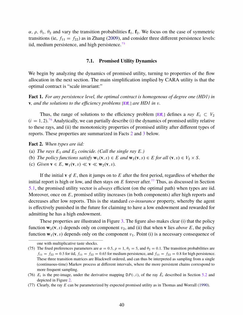
˛; �; �1; �2 and vary the transition probabilities f1; f2. We focus on the case of symmetric

transitions (ie, f11 D f22) as in Zhang (2009), and consider three different persistence levels:

iid, medium persistence, and high persistence.75

7.1. Promised Utility Dynamics

We begin by analyzing the dynamics of promised utility, turning to properties of the flow

allocation in the next section. The main simplification implied by CARA utility is that the

optimal contract is “scale invariant:”

Fact 1. For any persistence level, the optimal contract is homogenous of degree one (HD1) in

v, and the solutions to the efficiency problems [Effi ] are HD1 in v.

Thus, the range of solutions to the efficiency problem [Effi ] defines a ray Ei � V2

(i D 1; 2).76 Analytically, we can partially describe (i) the dynamics of promised utility relative

to these rays, and (ii) the monotonicity properties of promised utility after different types of

reports. These properties are summarized in Facts 2 and 3 below.

Fact 2. When types are iid:

(a) The rays E1 and E2 coincide. (Call the single ray E.)

(b) The policy functions satisfy w1.v; s/ 2 E and w2.v; s/ 2 E for all .v; s/ 2 V2 � S .

(c) Given v 2 E, w1.v; s/ � v � w2.v; s/.

If the initial v 62 E, then it jumps on to E after the first period, regardless of whether the

initial report is high or low, and then stays on E forever after.77 Thus, as discussed in Section

5.1, the promised utility vector is always efficient (on the optimal path) when types are iid.

Moreover, once on E, promised utility increases (in both components) after high reports and

decreases after low reports. This is the standard co-insurance property, whereby the agent

is effectively punished in the future for claiming to have a low endowment and rewarded for

admitting he has a high endowment.

These properties are illustrated in Figure 3. The figure also makes clear (i) that the policy

function w2.v; s/ depends only on component v2, and (ii) that when v lies above E, the policy

function w1.v; s/ depends only on the component v1. Point (i) is a necessary consequence of

one with multiplicative taste shocks.

(75) The fixed preferences parameters are ˛ D 0:5, � D 1, �1 D 5, and �2 D 0:1. The transition probabilities are

f11 D f22 D 0:5 for iid, f11 D f22 D 0:65 for medium persistence, and f11 D f22 D 0:8 for high persistence.

These three transition matrices are Blackwell ordered, and can thus be interpreted as sampling from a single

(continuous-time) Markov process at different intervals, where the more persistent chains correspond to

more frequent sampling.

(76) Ei is the pre-image, under the derivative mapping DP.�; i/, of the ray QEi described in Section 5.2 and

depicted in Figure 2.

(77) Clearly, the ray E can be parameterized by expected promised utility as in Thomas and Worrall (1990).

40

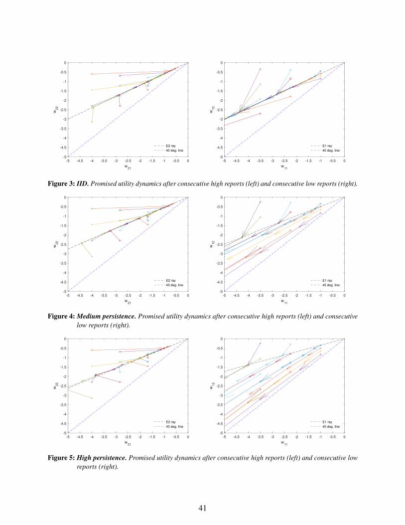
-5 -4.5 -4 -3.5 -3 -2.5 -2 -1.5 -1 -0.5 0

w21

-5

-4.5

-4

-3.5

-3

-2.5

-2

-1.5

-1

-0.5

0

w2

2

E2 ray

45 deg. line

-5 -4.5 -4 -3.5 -3 -2.5 -2 -1.5 -1 -0.5 0

w11

-5

-4.5

-4

-3.5

-3

-2.5

-2

-1.5

-1

-0.5

0

w1

2

E1 ray

45 deg. line

Figure 3: IID. Promised utility dynamics after consecutive high reports (left) and consecutive low reports (right).

-5 -4.5 -4 -3.5 -3 -2.5 -2 -1.5 -1 -0.5 0

w21

-5

-4.5

-4

-3.5

-3

-2.5

-2

-1.5

-1

-0.5

0

w2

2

E2 ray

45 deg. line

-5 -4.5 -4 -3.5 -3 -2.5 -2 -1.5 -1 -0.5 0

w11

-5

-4.5

-4

-3.5

-3

-2.5

-2

-1.5

-1

-0.5

0

w1

2

E1 ray

45 deg. line

Figure 4: Medium persistence. Promised utility dynamics after consecutive high reports (left) and consecutive

low reports (right).

-5 -4.5 -4 -3.5 -3 -2.5 -2 -1.5 -1 -0.5 0

w21

-5

-4.5

-4

-3.5

-3

-2.5

-2

-1.5

-1

-0.5

0

w2

2

E2 ray

45 deg. line

-5 -4.5 -4 -3.5 -3 -2.5 -2 -1.5 -1 -0.5 0

w11

-5

-4.5

-4

-3.5

-3

-2.5

-2

-1.5

-1

-0.5

0

w1

2

E1 ray

45 deg. line

Figure 5: High persistence. Promised utility dynamics after consecutive high reports (left) and consecutive low

reports (right).

41

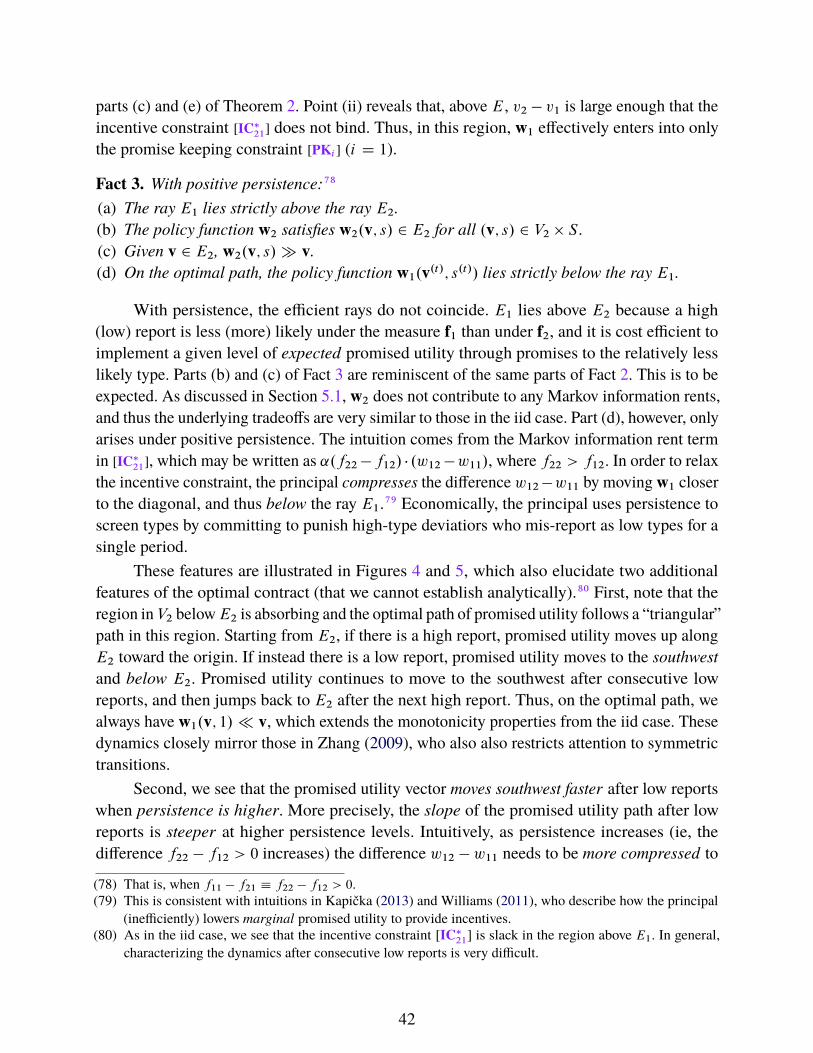
parts (c) and (e) of Theorem 2. Point (ii) reveals that, above E, v2 � v1 is large enough that the

incentive constraint [IC�21] does not bind. Thus, in this region, w1 effectively enters into only

the promise keeping constraint [PKi ] (i D 1).

Fact 3. With positive persistence:78

(a) The ray E1 lies strictly above the ray E2.

(b) The policy function w2 satisfies w2.v; s/ 2 E2 for all .v; s/ 2 V2 � S .

(c) Given v 2 E2, w2.v; s/ � v.

(d) On the optimal path, the policy function w1.v.t/; s.t// lies strictly below the ray E1.

With persistence, the efficient rays do not coincide. E1 lies above E2 because a high

(low) report is less (more) likely under the measure f1 than under f2, and it is cost efficient to

implement a given level of expected promised utility through promises to the relatively less

likely type. Parts (b) and (c) of Fact 3 are reminiscent of the same parts of Fact 2. This is to be

expected. As discussed in Section 5.1, w2 does not contribute to any Markov information rents,

and thus the underlying tradeoffs are very similar to those in the iid case. Part (d), however, only

arises under positive persistence. The intuition comes from the Markov information rent term

in [IC�21], which may be written as ˛.f22 �f12/ � .w12 �w11/, where f22 > f12. In order to relax

the incentive constraint, the principal compresses the difference w12 �w11 by moving w1 closer

to the diagonal, and thus below the ray E1.79 Economically, the principal uses persistence to

screen types by committing to punish high-type deviatiors who mis-report as low types for a

single period.

These features are illustrated in Figures 4 and 5, which also elucidate two additional

features of the optimal contract (that we cannot establish analytically).80 First, note that the

region in V2 belowE2 is absorbing and the optimal path of promised utility follows a “triangular”

path in this region. Starting from E2, if there is a high report, promised utility moves up along

E2 toward the origin. If instead there is a low report, promised utility moves to the southwest

and below E2. Promised utility continues to move to the southwest after consecutive low

reports, and then jumps back to E2 after the next high report. Thus, on the optimal path, we

always have w1.v; 1/ � v, which extends the monotonicity properties from the iid case. These

dynamics closely mirror those in Zhang (2009), who also also restricts attention to symmetric

transitions.

Second, we see that the promised utility vector moves southwest faster after low reports

when persistence is higher. More precisely, the slope of the promised utility path after low

reports is steeper at higher persistence levels. Intuitively, as persistence increases (ie, the

difference f22 � f12 > 0 increases) the difference w12 � w11 needs to be more compressed to

(78) That is, when f11 � f21 � f22 � f12 > 0.

(79) This is consistent with intuitions in Kapička (2013) and Williams (2011), who describe how the principal

(inefficiently) lowers marginal promised utility to provide incentives.

(80) As in the iid case, we see that the incentive constraint [IC�21] is slack in the region above E1. In general,

characterizing the dynamics after consecutive low reports is very difficult.

42

achieve the same schedule of information rents in the current period. This is a force that tends

to move w1 toward the diagonal. But this also leads to a tighter incentive constraint (ie, the

left-hand side of [IC�21]) in the next period. To compensate for this additional incentive cost,

the principal pushes the level of tomorrow’s promised utility down further.81 We can see this

more precisely by considering the time-series behavior of the following dual variables: (i)

the derivative DP.v; s/ D .P1.v; s/; P2.v; s// and (ii) the Lagrange multiplier �21.v; s/ � 0 on

[ICij ] (i D 2; j D 1). On the optimal path, they satisfy

[7.1]P1.v

.t/; s.t//

fs.t/;1

�P2.v

.t/; s.t//

fs.t/;2

MC of compression

D 1.s.t/ D 1/ �.f11 � f21/

fs.t/;1 � fs.t/;2

��21.v

.t�1/; s.t�1//

fs.t�1/;s.t/

MB of compression

The MC of compression is the Marginal Cost of moving the promised utility vector

toward the diagonal while holding ex ante promised utility Efs.t/�

v.t/�

constant. The MB of

compression is precisely the (shadow) Marginal Benefit of relaxing the preceding period’s

incentive constraint. Due to the cost smoothing motive (ie, convexity of P ), it is optimal

for the principal to have promised utility drift away from E1 gradually (ie, over multiple

periods) along strings of consecutive low reports. Holding the value of the weighted multiplier

�21.v.t�1/; s.t�1//=fs.t�1/;s.t/ fixed,82 the MB of compression indeed increases in persistence,

suggesting that promised utility should indeed drift away from E1 more quickly. While this

ignores the indirect effects of increased persistence on the dual variables, this intuition appears

to be borne out in the numerical examples.

The need to manage Markov information rents in this manner also introduces a new form

of history-dependence relative to the iid case. An important result in Thomas and Worrall

(1990) is that, when types are iid and utility is CARA, the order of reported types does not

matter:83

Fact 4. Suppose that types are iid and the initial v.0/ 2 E. Then, v.t/.h/ depends on the realized

length-t history of reports ht D .s1; : : : ; st/ only through the number of high and low reports,

but not the order in which they were made.84

This is easy to see from Facts 1 and 2. Because the policy functions are HD1 and

promised utility travels along the single ray E, there must exist numbers b1; b2 > 0 such

(81) This does not necessarily imply that ex ante promised utility decreases more quickly when persistence is

greater, as the slopes of the level sets of the form¶

v W Efs Œv� D M·

vary with the transition probabilities. But,

at least in these parametrized examples, it is the case that ex ante promised utility decreases more quickly

with persistence. This can be seen in the right-hand panels of Figures 6–8, where the “Ev” series illustrate

the dynamics of Efs.t/

�

v.t/�

.

(82) We show in [C.12] that this weighted multiplier does not depend on the value of s.t�1/.

(83) This fact is also implicit in Green (1987).

(84) Recall that sn denotes the type of report made in period n� 1, which then becomes part of the period n state

variable.

43

2 4 6

period

-1

-0.5

0

0.5

1

1.5

2

Ind. =1

2 4 6

period

-2

-1.5

-1

-0.5

0

u1

u2

V1

V2

2 4 6

period

-3

-2

-1

0

w11

w12

w21

w22

Ev

2 4 6

period

-1

-0.5

0

0.5

1

1.5

2

Ind. =1

2 4 6

period

-2

-1.5

-1

-0.5

0

u1

u2

V1

V2

2 4 6

period

-3

-2

-1

0

w11

w12

w21

w22

Ev

Figure 6: IID. Short-run dynamics along two report sequences.

2 4 6

period

-1

-0.5

0

0.5

1

1.5

2

Ind. =1

2 4 6

period

-2.5

-2

-1.5

-1

-0.5

0

u1

u2

V1

V2

2 4 6

period

-3

-2

-1

0

w11

w12

w21

w22

Ev

2 4 6

period

-1

-0.5

0

0.5

1

1.5

2

Ind. =1

2 4 6

period

-2.5

-2

-1.5

-1

-0.5

0

u1

u2

V1

V2

2 4 6

period

-3

-2

-1

0

w11

w12

w21

w22

Ev

Figure 7: Medium persistence. Short-run dynamics along two report sequences.

2 4 6

period

-1

-0.5

0

0.5

1

1.5

2

Ind. =1

2 4 6

period

-2.5

-2

-1.5

-1

-0.5

0

u1

u2

V1

V2

2 4 6

period

-4

-3

-2

-1

0

w11

w12

w21

w22

Ev

2 4 6

period

-1

-0.5

0

0.5

1

1.5

2

Ind. =1

2 4 6

period

-2.5

-2

-1.5

-1

-0.5

0

u1

u2

V1

V2

2 4 6

period

-4

-3

-2

-1

0

w11

w12

w21

w22

Ev

Figure 8: High persistence. Short-run dynamics along two report sequences.

44

that wi.v; s/ D bi � v whenever v 2 E. Thus, under the hypotheses of Fact 4, it must be

that v.t/ D bN .t/

1 � bt�N .t/

2 � v0 where N .t/ is the (random) number of low reports in periods

0; 1; : : : ; t � 1. Thus, the order of reports does not matter. This is illustrated in Figure 6, which

plots the time-series behavior of promised utility and the policy functions along two report

sequences, each of which have three low reports and three high reports but differ in the order.85

In the terminal period, t D 7, we see that v.7/ is the same across the two sequences, as are the

flow utility policy functions ui.v.7/; s.7//.

The intuition for this order-independence result in Thomas and Worrall (1990) is based

on the absence of wealth effects under CARA utility. But, as illustrated in Figures 7 and 8,

this result also depends critically on the assumption of iid types. In both figures, we see that

the terminal promised utility vector and policy functions for flow utility end up lower when

the low reports occur earlier in the sequence. Moreover, this effect is quantitatively larger

in the high persistence case.86 This appears to be driven by the following feature: if, after

multiple consecutive low reports the next report is high, then the promised utility vector jumps

back to E2 by moving to the northwest. (See the left-hand panel of Figure 5 and the v.t/ time

series in the right-hand panel of Figure 8.) That is, when v is far enough below E2, we have

w22.v; 1/ > v2 whilew21.v; 1/ < v1. Thus, promised utility for low endowment types continues

to decrease even after the first high endowment report, therefore increasing the difference

w22.v; 1/ � w21.v; 1/. We have argued above that, with persistence, the incentive constraint

effectively tightens after consecutive low reports. Here, we see that it is evidently optimal to

re-introduce slack into [IC�21] after the first high report. Thus, it matters whether a given high

report is preceded by a high or low report.

7.2. Wedge Dynamics

Next, we turn to the dynamics of the flow utilities and the insurance properties of the optimal

contract. A standard way to characterize allocative distortions in settings with non-transferable

utility is via wedges that represent departures from the first-best allocation. While not emphas-

ized in the early work on risk sharing, these are the main objects of study in the literature

optimal dynamic taxation.

Definition 7.1. The wedges are defined as follows:87

(85) The initial condition for v is drawn from the ray E2 in each of Figures 6–8.

(86) In these examples, only the terminal values of v.7/i and ui .v

.7/; s.7// for i D 1 are noticeably different across

the two sequences. We have generated other (unreported) examples in which all of the terminal variables

depend on the report order.

(87) These definitions are the same as those in Zhang (2009). Some papers use slightly different, but equivalent,

definitions of the wedges. For example, Farhi and Werning (2013) refer to Wint=.Wint C 1/ as the “inter-

temporal wedge,” and Golosov, Troshkin and Tsyvinski (2016) refer to the same object as the “savings

distortion.”

45

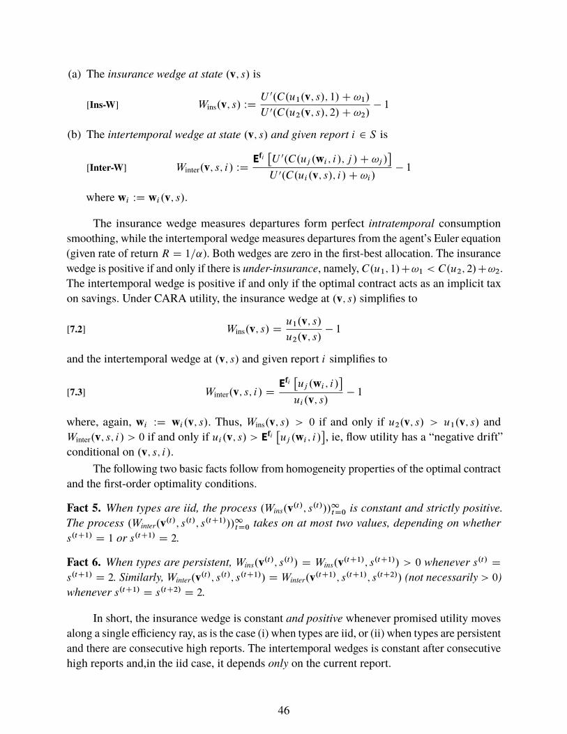
(a) The insurance wedge at state .v; s/ is

[Ins-W] Wins.v; s/ WDU 0.C.u1.v; s/; 1/C !1/

U 0.C.u2.v; s/; 2/C !2/� 1

(b) The intertemporal wedge at state .v; s/ and given report i 2 S is

[Inter-W] Winter.v; s; i/ WDEfi�

U 0.C.uj .wi ; i/; j /C !j /�

U 0.C.ui.v; s/; i/C !i/� 1

where wi WD wi.v; s/.

The insurance wedge measures departures form perfect intratemporal consumption

smoothing, while the intertemporal wedge measures departures from the agent’s Euler equation

(given rate of return R D 1=˛). Both wedges are zero in the first-best allocation. The insurance

wedge is positive if and only if there is under-insurance, namely, C.u1; 1/C!1 < C.u2; 2/C!2.

The intertemporal wedge is positive if and only if the optimal contract acts as an implicit tax

on savings. Under CARA utility, the insurance wedge at .v; s/ simplifies to

[7.2] Wins.v; s/ Du1.v; s/

u2.v; s/� 1

and the intertemporal wedge at .v; s/ and given report i simplifies to

[7.3] Winter.v; s; i/ DEfi�

uj .wi ; i/�

ui.v; s/� 1

where, again, wi WD wi.v; s/. Thus, Wins.v; s/ > 0 if and only if u2.v; s/ > u1.v; s/ and

Winter.v; s; i/ > 0 if and only if ui.v; s/ > Efi�

uj .wi ; i/�

, ie, flow utility has a “negative drift”

conditional on .v; s; i/.

The following two basic facts follow from homogeneity properties of the optimal contract

and the first-order optimality conditions.

Fact 5. When types are iid, the process .Wins.v.t/; s.t///1tD0 is constant and strictly positive.

The process .Winter.v.t/; s.t/; s.tC1///1tD0 takes on at most two values, depending on whether

s.tC1/ D 1 or s.tC1/ D 2.

Fact 6. When types are persistent, Wins.v.t/; s.t// D Wins.v

.tC1/; s.tC1// > 0 whenever s.t/ D

s.tC1/ D 2. Similarly, Winter.v.t/; s.t/; s.tC1// D Winter.v

.tC1/; s.tC1/; s.tC2// (not necessarily > 0)

whenever s.tC1/ D s.tC2/ D 2.

In short, the insurance wedge is constant and positive whenever promised utility moves

along a single efficiency ray, as is the case (i) when types are iid, or (ii) when types are persistent

and there are consecutive high reports. The intertemporal wedges is constant after consecutive

high reports and,in the iid case, it depends only on the current report.

46

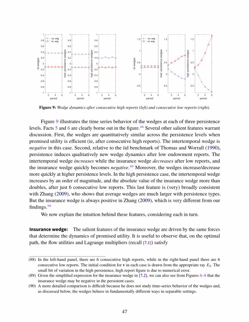
2 4 6

period

-1

-0.8

-0.6

-0.4

-0.2

0

0.2

0.4

0.6

0.8

1

iid w

ed

ge

sins. wdg

int. wdg

2 4 6

period

-1

-0.8

-0.6

-0.4

-0.2

0

0.2

0.4

0.6

0.8

1

me

d.

pe

rsis

ten

ce

we

dg

es

2 4 6

period

-1

-0.8

-0.6

-0.4

-0.2

0

0.2

0.4

0.6

0.8

1

hig

h p

ers

iste

nce

we

dg

es

2 4 6

period

-0.5

0

0.5

1

1.5

iid w

ed

ge

s

ins. wdg

int. wdg

2 4 6

period

-0.5

0

0.5

1

1.5

me

d.

pe

rsis

ten

ce

we

dg

es

2 4 6

period

-0.5

0

0.5

1

1.5

hig

h p

ers

iste

nce

we

dg

es

Figure 9: Wedge dynamics after consecutive high reports (left) and consecutive low reports (right).

Figure 9 illustrates the time series behavior of the wedges at each of three persistence

levels. Facts 5 and 6 are clearly borne out in the figure.88 Several other salient features warrant

discussion. First, the wedges are quantitatively similar across the persistence levels when

promised utility is efficient (ie, after consecutive high reports). The intertemporal wedge is

negative in this case. Second, relative to the iid benchmark of Thomas and Worrall (1990),

persistence induces qualitatively new wedge dynamics after low endowment reports. The

intertemporal wedge increases while the insurance wedge decreases after low reports, and

the insurance wedge quickly becomes negative.89 Moreover, the wedges increase/decrease

more quickly at higher persistence levels. In the high persistence case, the intertemporal wedge

increases by an order of magnitude, and the absolute value of the insurance wedge more than

doubles, after just 6 consecutive low reports. This last feature is (very) broadly consistent

with Zhang (2009), who shows that average wedges are much larger with persistence types.

But the insurance wedge is always positive in Zhang (2009), which is very different from our

findings.90

We now explain the intuition behind these features, considering each in turn.

Insurancewedge: The salient features of the insurance wedge are driven by the same forces

that determine the dynamics of promised utility. It is useful to observe that, on the optimal

path, the flow utilities and Lagrange multipliers (recall [7.1]) satisfy

(88) In the left-hand panel, there are 6 consecutive high reports, while in the right-hand panel there are 6

consecutive low reports. The initial condition for v in each case is drawn from the appropriate ray E2. The

small bit of variation in the high persistence, high report figure is due to numerical error.

(89) Given the simplified expression for the insurance wedge in [7.2], we can also see from Figures 6–8 that the

insurance wedge may be negative in the persistent cases.

(90) A more detailed comparison is difficult because he does not study time-series behavior of the wedges and,

as discussed below, the wedges behave in fundamentally different ways in separable settings.

47

C 0�

u2.v.t/; s.t//; 2

�

� C 0�

u1.v.t/; s.t//; 1

�

direct MC of " Wins.v.t/; s.t//

D

�

fs.t/;1

fs.t/;2

C�2

�1

�

��.v.t/; s.t//

fs.t/;1

MB of " Wins.v.t/; s.t//

� 1.s.t/ D 1/ �.f11 � f21/

fs.t/;1 � fs.t/;2

��21.v

.t�1/; s.t�1//

fs.t�1/;s.t/

indirect MC of " Wins.v.t/; s.t//

[7.4]

Increasing the insurance wedge always leads to a direct MC (on the left-hand side of

[7.4]), which corresponds to the departure from first-best risk-sharing. For any degree of

persistence, increasing the insurance wedge also adds slack to the incentive constraint [ICij ]

(i D 2; j D 1). In the iid case, these are the only two operative forces, and they lead to a

positive insurance wedge or, equivalently, under-insurance. When types are persistent, the

presence of Markov information rents introduces a countervailing force, represented by the

indirect MC of increasing the insurance wedge on the right-hand side of [7.4]. Notice that

this term is identical to the MB of compression (of contingent promised utilities) in [7.1].

Roughly speaking, one way to compress the difference w12.v.t�1/; s.t�1//�w11.v

.t�1/; s.t�1// is

to compress the difference u2.w1.v.t�1/; s.t�1//; 1/ � u1.w1.v

.t�1/; s.t�1//; 1/. That is, provide

more intratemporal insurance — ie, decrease the insurance wedge — at date t , contingent on a

date t � 1 low report (equivalently, s.t/ D 1). When this force is strong enough, as is the case

after consecutive low reports, the optimal contract over-insures the agent by specifying flow

allocations u1 > u2 and, equivalently, Wins < 0. These features can be seen in Figures 7–8 and

Figure 9, respectively. As we argued heuristically in Section 7.1, the indirect MC term in 7.4

suggests that these effects should be larger when persistence is higher. Indeed, this is precisely

what we see in the computed numerical examples.

It is useful to compare these insurance wedge dynamics to the findings of Farhi and

Werning (2013), who study the dynamics of the labour wedge in (both separable and non-

separable) productivity shock models of optimal dynamic taxation. Their central finding is

that, roughly speaking, the labour wedge inherits the same mean-reversion properties as the

productivity shock process. While direct comparisons are difficult given the differences in

settings,91 our results seem to be broadly consistent with theirs. In particular, our insurance

wedge does exhibit a kind of mean reversion: it becomes negative after consecutive low reports,

but becomes positive again (and the process “renews”) after a high report. Moreover, the

indirect MC term in [7.4] — and thus the size of the insurance wedge — depends directly on the

degree of persistence f11 �f21, which is akin to their result that the labour wedge mean-reverts

at the same rate as the underlying type process.

(91) Aside from considering a different class of preferences, source of private information, and type of wedge,

they also assume that types are continuously distributed and pay special attention to the case where the

logarithm of the productivity parameter follows an OU process.

48

Intertemporal wedge: To understand the sign of the intertemporal wedge, recall that prom-

ised utility drifts up (to the northeast, in Figures 3–5) after consecutive high reports, and down

(to the southwest) after consecutive low reports. This suggests that, conditional on receiving

a high endowment, the agent should expect his consumption to have “positive drift” in the

short run; conversely, receiving a low endowment should imply consumption to have short

run “negative drift.” Figures 6–8 show that this is indeed the case in our examples. Thus, the

intertemporal wedge is negative at high endowment reports because the agent would like to

borrow in the face of an upward-sloping consumption profile, and it is negative at low endow-

ment reports because the agent wants to save in the face of a downward-sloping consumption

profile.92

The fact that the intertemporal wedge increases after consecutive low reports is a con-

sequence of the same forces underlying the dynamics of promised utility discussed above. To

optimally manage Markov information rents, consumption has a more negative drift after low

reports when persistence is higher. This is compounded by the fact that persistence implies

that the agent puts more weight on the event of having another low endowment shock in the

next period.

This contrasts sharply with the separable productivity shock model (as in Zhang (2009)),

which always has a positive intertemporal wedge due to the IEE.93 Golosov, Kocherlakota

and Tsyvinski (2003) also emphasize that negative intertemporal distortions can arise in

pure insurance models (though their example is based on an extreme form of persistence),

while Golosov, Troshkin and Tsyvinski (2016) make a similar observation for non-separable

productivity shock models.94 The difference is that, in the separable model, consumption utiles

serve as a “type-independent numeraire,” much like money in quasi-linear models. The IEE

represents the optimal allocation of this numeraire over time, given the principal’s convex cost

function (the inverse of consumption utility). Outside of the separable model, the timing of

consumption is an important screening device, so cost smoothing and incentive provision are

inextricably linked.

(92) The reader can verify that, in the iid case, this feature is implied by the analytical solution from Proposition

6 in Thomas and Worrall (1990), at least when endowments are variable enough (ie, when !2 � !1 > 0 is

sufficiently large). Details are available upon request.

(93) It seems that many intuitions in the broader literature are based on this positive intertemporal wedge result,

even though it is special to the separable model. Albanesi and Armenter (2012), for example, emphasize the

importance of “permanent intertemporal distortions,” meaning an intertemporal wedge that does not change

sign along the optimal path. Clearly, our pure insurance model does not have this feature.

(94) In particular, it involves increasing impulse response functions (in the language of Pavan, Segal and Toikka

(2014)). Similarly, the intertemporal wedge is always negative in the hidden endowment example in Williams

(2011), where impulse responses are constant. (He finds that consumption has positive drift, and marginal

utility is a convex function of consumption.) Golosov, Troshkin and Tsyvinski (2016) show that “lifetime”

savings distortions must be positive in a broad class of non-separable productivity shock models, but this

result hinges on the assumption of a finite time horizon.

49

7.3. Intertemporal Cost-Smoothing

It is useful to take a more detailed look at how (i) persistence of private information and (ii) the

absence of a “type-independent numeraire” shape the principal’s intertemporal cost smoothing

at the optimum. With CARA utility, 0.u; 2; 1/ D �2=�1. Fix some .v; s/ and consider the cost

of increasing ex ante promised utility Efs Œv� by some amount " > 0. Recall from Section 5.1

that the martingale property of D1P.v; s/ in Proposition 5.1 is based on perturbing each of the

wi in direction " � 1 while leaving the flow utilities ui unchanged. We consider two different

perturbations here.

The first perturbation, which also changes v to v0 WD v C "1, is to increase each of the

flow utilities ui by " but leave the wi unchanged. This must be locally optimal by the envelope

theorem, giving us the formula

[7.5] D1P.v; s/ D Efs�

C 0.ui ; i/�

direct cost

�

�

1 ��2

�1

�

� �.v; s/

incentive cost

where �.v; s/ � 0 is a Lagrange multiplier on the incentive constraint [ICij ] (i D 2; j D 1).

Notice that, because C 0.ui ; i/ D 1=U 0.ci C !i/, the first “direct cost” term on the right is

actually the agent’s expected inverse marginal utility. If expected inverse marginal utility were

a martingale, it would be reminiscent of (but distinct from) the IEE. However, this this object

does not satisfy the martingale property because the underlying perturbation gives different

deviation incentives to each type. To understand the second “incentive cost” term on the right,

note that this perturbation increases the left-hand side of the incentive constraint [ICij ] (i > j )

by " while increasing the right-hand side by approximately 0.uj ; i; j / � " D .�i=�j / � " < ".

Thus, it adds total slack 1 � �i=�j to [ICij ], and the second term in [7.5] collects the marginal

(shadow) cost reduction achieved by relaxing the incentive constraints in this way.

Second, there is a different way to perturb (only) flow utilities that leaves the slack in

the current period’s incentive constraints invariant. Consider perturbing each ui to u0i WD

ui C "�i=Efs�

�j�

. It is easy to see that this increases each side of the [ICij ] equally and perturbs

v to v0 WD v C " � O�s, where for each s 2 S , the vector O�s 2 RdCC has i th component �i=E

fs�

�j�

.

Clearly, Efs Œv0 � v� D ", as desired. The marginal cost of such a perturbation is, after a short

calculation,

[7.6] D O�sP.v; s/ D Efs

�

C 0.ui ; i/�

(expected) inverse maringal utility

CCovfs Œ�i ; C

0.ui ; i/�

Efs Œ�i �

incentive provision

The second term on the right vanishes under the first-best, where the flow utility process is

constant, and thus measures the cost of incentive provision.

How are these perturbations connected? It turns out that they are both optimal when

types are iid, but the second is not optimal when types are persistent. Recall the cost function

50

K.v; s/ from the efficiency problem [Effi ] from Section 5.1, which coincides with the value

function from Thomas and Worrall (1990) when types are iid.

Lemma 7.2. Suppose that the agent has CARA utility and the Markov process satisfies MLRP.

Let .v.t/; s.t//1tD0 be the process induced by the optimal contract. Let v.t/ WD Efs.t/�

v.t/�

.

(a) If types are iid, then

K 0.v.t/; s.t// D D1P.v.t/; s.t// D D O�

s.t/P.v.t/; s.t//

and thus the process�

D O�s.t/P.v.t/; s.t//

�1

tD0is a martingale.

(b) If types are not iid, then

D O�s.t/P.v.t/; s.t// � D1P.v

.t/; s.t//

and the process�

D O�s.t/P.v.t/; s.t//

�1

tD0is not a martingale.

The proof of Lemma 7.2 is in Appendix C.4. This gives one sense in which the TW

martingale K 0.v.t/; s.t// and the differential martingale are not equivalent. In the iid setting,

optimal intertemporal cost-smoothing can be achieved by perturbations different from those

underlying the differential martingale. But these perturbations are not guaranteed to be optimal

(ie, induce a process satisfying the martingale property) outside the iid case. Intuitively, the

perturbation underlying the process D O�sP.v; s/ does not take into account the principal’s need

to manage Markov information rents.

8. Concluding Remarks

We close with just a few remarks regarding directions for future research. First, we argued in

Section 6.2 that ergodicity and asymptotically-vanishing impulse response functions appear

to be the critical properties of the type process that determine the long-run properties of the

optimal contract — namely, whether or not Absolute Immiseration occurs. While Theorem

3 helped us go some way toward making this case, much remains to be done. A definitive

answer to our conjecture seems to be important for a more complete understanding of optimal

insurance in private information economies. But, given the generality of the present analysis,

it seems that new techniques will be needed to tackle these questions.

Second, it seems important to better understand how the behavior of the wedges differ

between the kind of pure insurance setting studied here and the redistribution problem con-

sidered in optimal dynamic taxation. Our findings in Section 7 make some progress in this

direction, but perhaps more analytical progress could be made using the FOA in a model with

continuous types and continuous time.

Finally, many of our techniques — namely, the arguments behind the domain characteriz-

ation in Theorem 1 and the convergence proof in Theorem 3 — apply directly to other models

51

of dynamic contracting with Markovian types. For example, they can be used to generalize

the corresponding results in the firm financing model of Fu and Krishna (2017) and the re-

peated procurement model of Krasikov and Lamba (2018), thus paving the way for a deeper

understanding of dynamic incentives in these settings.

Appendices

The appendices are organized as follows. Appendix A contains the proof of Theorem 1. Appendix

B contains proofs from Section 5, including the proofs for Proposition 5.1, Theorem 3, and Theorem 4.

Appendix C contains proofs and derivations for the material in Section 7.

A Supplementary Appendix contains additional proofs and results. Material pertaining to the

sequential problem, [SP], and its relation to the recursive problem, [RP], is relegated to Supplementary

Appendix S.1.1. Supplementary Appendix S.2 contains details pertaining to the first-best problem from

Section 4.1. Supplementary Appendix S.3 contains all other proofs from Section 4, including that of

Theorem 2. Finally, Supplementary Appendices S.4 and S.5 contain auxiliary results used in the proofs

of Theorems 1 and 3, respectively.

A. Proofs Concerning the Recursive Domain

Appendix A, which is divided into several parts, is concerned with proving Theorem 1. Appendix A.1

introduces the operator Bı, of which D is the largest fixed point, and establishes basic existence and

characterization results concerning D, D�, and �.�/. The heart of the proof is contained in the various

parts of Appendix A.2, which is focused mainly on two auxiliary operators, B and B�. First, Appendix

A.2.1 establishes several results relating fixed points of the three operators to each other and to the set

Vd . Second, Appendices A.2.2 and A.2.3 focus on the special case of CARA utility. Appendix A.2.2

characterizes iterates of B� via solutions to an appropriate linear program and its dual, and culminates in

closed-form expressions for these iterates when the Markov process satisfies MLRP or PPR. Appendix

A.2.3 characterizes iterates of B via solutions to an appropriate conic program and its dual (which are

not characterized in closed form). Third, Appendix A.2.4 returns to the case of general DARA utility

functions and, using a Lagrangian argument, shows that this actually reduces to the CARA case studied

in Appendix A.2.3. Finally, Appendix A.3 collects these various pieces into a proof of Theorem 1.

A.1. Preliminary Observations

We begin with an elementary lemma concerning the .�; i; j / functions.

Lemma A.1. Let i; j 2 S with i > j . Under Assumption DARA:

(a) .u; i; j / is convex, 0.u; i; j / 2 .0; 1/, and .u; i; j / > u for all u 2 U.

52

(b) The extension of .�; i; j / to R� given by .0; i; j / WD 0 and 0.0; i; j / WD 1 preserves continuity,

convexity, and continuous differentiability.

(c) a .u; i; j / � .au; i; j / for all u 2 U and a 2 Œ0; 1�.

(d) Under CARA utility, .u; i; j / D .�i=�j / � u where �k WD e�!k for all k 2 S . Thus, a .u; i; j / D

.au; i; j / for all u 2 U and a 2 RC.

Proof. By the Inverse Function Theorem, we get

[A.1] 0.u; i; j / DU 0.!i C C.u; j //

U 0.!j C C.u; j //> 0

It follows immediately from part (a) of Assumption DARA that .u; i; j /�u > 0 and 0.u; i; j / 2 .0; 1/.

Moreover, we have

log�

0.u; i; j /�

D log�

U 0.!i C C.u; j //�

� log�

U 0.!j C C.u; j //�

and because C.�; j / is strictly increasing, by part 3 of Assumption DARA, log . 0.u; i; j // is increasing.

It follows that 0.u; i; j / is increasing, ie, .�; i; j / is convex.

For part (b), note that, since the consumption domain Cis assumed unbounded above, limu!0 .u; i; j / D

limu!0 U .!i C C.u; j // D limc!1 U.!i C c/ D 0. Thus this extension preserves continuity and con-

vexity of .�; i; j /. Moreover, taking the limit u ! 0 in [A.1] delivers 0.0; i; j / D 1.

For part (c), let u 2 U and a 2 Œ0; 1�. We have .au; i; j / � a .u; i; j / C .1 � a/ .0; i; j / D

a .u; i; j /, where the inequality is from convexity and the equality is from .0; i; j / D 0, shown above.

Part (d) is immediate from the definitions.

Recall that the set of recursive constraints consists of the of the promise keeping conditions

[PKj ] uj C ˛ Efj�

wj

�

D vj

for all j 2 S , and the incentive compatibility conditions

[ICij ] .uj ; i; j /C ˛ Efi�

wj

�

� vi

for all i; j 2 S with i > j .

For any v 2 Ud , we say that the menu .u;w/ WD .ui ;wi /i2S 2�

R� � Rd�

�d(where u WD

.u1; : : : ; ud / and w WD .w1; : : : ;wd /) implements v if it satisfies all of the recursive constraints at v.

(Note that implementation does not require even that ui < 0 or wi � 0. Such feasibility requirements

will be included as separate constraints.) Consider — in the manner of Abreu, Pearce and Stacchetti

(1990) — the operator Bı W 2Ud

! 2Ud

, defined as follows for any K � Ud :

Bı.K/ WD¶

v 2 Ud W 9 .u;w/ that implements v with .ui ;wi / 2 U�K for all i 2 S

·

[A.2]

Recalling Definition 3.1, it is easy to see that any fixed point of Bı is a recursive domain, and that the

largest recursive domain D is precisely the largest fixed point of the operator Bı.

Define the correspondence � W Ud � Kd ⇒

�

U� Ud�d

by

[A.3] �.v; K/ WD¸

.u;w/ 2 .U�K/d W .u;w/ implements v¹

53

Thus �.v/, defined in [3.1] in the main text, is equal to �.v;D/. Clearly, an alternative way of defining

the operator in [A.2] is Bı.K/ D¸

v 2 Ud W �.v; K/ ¤ ∅

¹

.

Say that set K � Rd has decreasing returns if v 2 K implies that av 2 K for all a 2 .0; 1�. Say

that a set K � Rd is unbounded below if, for all r < 0, there exists v 2 K such that v � r1.

Lemma A.2. Let K � Ud . Then:

(a) If K is convex, then �.�; K/ has convex graph.

(b) If K has decreasing returns, then the graph of �.�; K/ has decreasing returns.

(c) If K is a cone and utility is CARA, then the graph of �.�; K/ is a cone.

Proof. For part (a), suppose that K is convex and let 2 �.v; K/ and 0 2 �.v0; K/. Let a 2 .0; 1/ and

define v00 WD av C .1�a/v0 2 Ud and 00 WD a C .1�a/ 0 2 .U�K/d . Each of the [PKj ] constraints

is linear, so clearly 00 satisfies all of them at v00. Consider constraint [ICij ], with i > j . By definition

of and 0, we have

v00i � a .uj ; i; j /C .1 � a/ .u0

j ; i; j /C ˛ Efi

h

awj C .1 � a/w0j

i

and, since .�; i; j / is convex by part (a) of Lemma A.1, a .uj ; i; j /C .1� a/ .u0j ; i; j / � .u00

j ; i; j /.

Thus, 00 satisfies [ICij ] at v00. Hence, 00 2 �.v00; K/, ie, �.�; K/ has convex graph when K is convex.

For part (b), suppose that K has decreasing returns and let 2 �.v; K/. Let a 2 .0; 1/ and define

v0 WD av 2 Ud and 0 WD a 2 .U�K/d . Each of the [PKj ] constraints is linear, so clearly 0 satisfies

all of them at v0. Consider constraint [ICij ], with i > j . By definition of , we have

v0i � a .uj ; i; j /C ˛ Efi

�

awj

�

and, by part (c) of Lemma A.1, a .uj ; i; j / � .auj ; i; j /. Thus, 0 satisfies [ICij ] at v0. Hence,

0 2 �.v0; K/, ie, �.�; K/ has graph with decreasing returns when K has decreasing returns.

For part (c), mimic the proof of part (b) above, invoking part (d) of Lemma A.1 instead of part

(c) of that lemma.

Proposition A.3. The following hold:

(a) There exists a largest recursive domain D. It is nonempty, convex, has decreasing returns, and is

unbounded below.

(b) D� � D has all of the above properties.

(c) The constraint correspondence � W D ! .U�D/d is nonempty-valued, has convex graph, and is

continuous.

Proof. Begin with part (a). It is easy to see that the operator Bı is monotone increasing with respect to

set inclusion. Because�

2Ud

;��

defines a complete lattice, Bı has a largest fixed point D by Tarski’s

Fixed Point Theorem.

To establish that D is nonempty and unbounded below, define

B WD fc 2 R W c C !i 2 C8i 2 Sg

Clearly inf B D c � !1 and supB D C1. For any c 2 B , let vc 2 Ud denote the vector of contingent

promised utilities induced by the stochastic consumption process�

!.t/ C c�1

tD0. (Thus, v0 is the

54

promised utility vector under autarky.) Define Dc WD fvcg for each c 2 B. It is easy to see that

Bı .Dc/ D Dc , and thus [c2BDc � D, for each c 2 B . Since U� R��, it follows that

vci � U.!1 C c/ � T1

for all i 2 S , where

T1 WD E

"

1X

tD0

˛t1.s.tC1/ D 1/ˇ

ˇs.0/ D i

#

and T1 > 0 by Assumption Markov. Moreover, limc!inf B U.!1 C c/ D �1 under Assumption DARA.

Thus, for any r 2 R��, there exists c 2 B such that maxi2S vci < r . Thus, [c2BDc is unbounded

below. Now, it follows from the definition of D that D � [c2BDc . It follows that D is nonempty and

unbounded below.

We now proceed to establish convexity and decreasing returns. Define Kcdrd

� 2Ud

to be the

collection of all subsets of Ud that are convex and have decreasing returns. It is easy to see that Kcdrd

is a complete lattice, with the meet operation defined by set intersection and the join operation defined

by the natural notion of “convex, decreasing-returns hull,” namely

_

�2ƒ

K� WD\

¼

K 2 Kcdrd W K �

[

�2ƒ

K�

½

It follows from Lemma A.2 that Bı W Kcdrd

! Kcdrd

is well-defined and monotone increasing.Thus, by

Tarski’s Fixed Point Theorem, Bı has a largest fixed point D0 2 Kcdrd

. But since Ud 2 Kcdrd

, it is easy

to see that D 2 Kcdrd

and hence D D D0. (See, eg, the transfinite recursion in Lemma 1 of Echenique

(2005).) This concludes the proof of part (a).

Now consider part (b). Define scalar multiplication and convex combination of recursive contracts

pointwise. It follows from the definition that if � satisfies agent transversality at v 2 D, then for any

a > 0, a� satisfies agent transversality at av 2 D. Similarly, if � and � 0 satisfy agent transversality at,

respectively, v 2 D and v0 2 D, then for any a 2 .0; 1/, a� C .1 � a/� 0 satisfies agent transversality at

av C .1 � a/v0. It follows from these observations and the fact that D is convex and has decreasing

returns, which was established in part (a), that D� inherits both of these properties. Moreover, the

vectors vc defined in the proof of part (a) are clearly elements of D�, which establishes that D� is

nonempty and unbounded below.

Finally, consider part (c). This follows immediately from part (a) of the present proposition

and part (a) of Lemma A.2, namely the facts that D is convex and �.�/ D �.�;D/ as defined in [A.3].

Continuity is easy to see from the definitions.

A.2. Fixed Points of Operators

While we are ultimately interested in (largest) fixed points of Bı, it is convenient to work with some

auxiliary operators. Consider first the operator B, defined as follows for any K � Rd�:

B.K/ WD¶

v 2 Rd� W 9 .u;w/ that implements v with .ui ;wi / 2 R� �K for all i 2 S

·

[A.4]

55

It is easy to see that Bı.K/ � B.K/ for all K, so that the largest fixed point of Bı is a subset of the

largest fixed point of B. To compute the largest fixed point of B, consider in turn the family of operators

defined as follows for any K � Ud :

Bij .K/ WD¶

v 2 Rd� W 9 .uj ;wj / 2 R� �K s.t. [PKj ] and [ICij ] hold at v

·

[A.5]

Notice that for any set K, we have

B.K/ D\

i;j 2S W i>j

Bij .K/

We may also use the Bij to define a further auxiliary operator B� W 2Rd� ! 2R

d� as

B�.K/ D

d�1\

j D1

Bj C1;j .K/

where Bj C1;j is defined in [A.5]. It is easy to see that B.K/ � B�.K/ for all K, so that the largest

fixed point of B is a subset of the largest fixed point of B�.

We note the following property for future reference. Let K� 2Rd� denote the collection of subsets

K � Rd� that are closed convex cones.

Lemma A.4. Suppose utility is CARA. The maps B W K! K and B� W K! K are well-defined.

Proof. Immediate from part (c) of Lemma A.2 and the definition of the constraint correspondence �.�/

(see [3.1]).

A.2.1. Some Fixed Points

Let Vd WD fv 2 Rd� W v1 < v2 < � � � < vd g and let clVd denote its closure; thus, clVd D fv 2

Rd� W v1 � v2 � � � � � vd g. We claim that, if the Markov process satisfies FOSD, B.clVd / D clVd ,

Bı.clVd / D Vd , and that Bı.Vd / D Vd . We establish these facts below.

Lemma A.5. Consider [PKj ] and [ICij ] where i > j and let v 2 clVd .

(a) Suppose the Markov process satisfies FOSD. Suppose, in addition, that vi D vj . Any solution to

[PKj ] and [ICij ] with wj 2 cl Vd must satisfy uj D 0 and Efi Œwj � D Efj Œwj �.

(b) In general, if vj C1 > vj , there exist uj < 0 and wj 2 clVd with wj � 0 such that [PKj ] holds and

[ICij ] holds as a strict inequality for all i > j . In particular, there exists such a solution in which

wj D wj 1 for some wj < 0.

Proof. To see (a), let .uj ;wj / satisfy both [PKj ] and [ICij ]. Subtract [PKj ] from each side of [ICij ] to

obtain

0 � .uj ; i; j / � uj C ˛�

Efi Œwj � � Efj Œwj �

�

� vi � vj D 0

Recall from Lemma A.1 that .u; i; j / > u for all u 2 U and .0; i; j / D 0. Moreover, Efi Œwj � �

Efj Œwj � because wj 2 cl Vd and fi first-order stochastically dominates fj . Thus, the above display

implies that uj D 0 and Efi Œwj � D Efj Œwj �.

56

To see (b), notice that setting uj D 0 and wj D wj 1 withwj D vj =˛ means that [PKj ] holds as an

equality, while [ICij ] holds as a strict inequality for all i > j (because vj C1 > vj and v 2 clVd ). Now,

increasewj by a small amount while reducing uj simultaneously to ensure that [PKj ] still holds. Because

all the constraints [ICij ] held as strict inequalities, this perturbation also satisfies these constraints as

strict inequalities.

Lemma A.6. Fix wj < 0. Then, for all " > 0, there exists wj 2 Vd such that (i) Efj Œwj � D wj , and (ii)

Efi Œwj � � Efj Œwj � < " for all i > j . If the Markov process satisfies FOSD, there exists wj 2 Vd that

satisfies (i), (ii) , and (iii) Efi Œwj � � Efj Œwj �.

Proof. Fix Q" > 0 as a parameter to be optimised later. Let wjk WD wj � Q"=2k for k D 1; : : : ; d � 1, and

wjd WD wj C ı, where ı WD Q"fjd

Pd�1kD1 fjk=2

k . It is easy to see that Efj Œwj � D wj , establishing (i).

To see (ii), note that Efi Œwj ��Efj Œwj � � wjd �wj1 D ıC Q" D Q"

fjd

h

Pd�1kD1 fjk=2

k C fjd

i

< Q"=fjd .

So by choosing Q" D " � fjd , we establish (ii).

If the Markov process satisfies FOSD, it follows immediately that Efi Œwj � � Efj Œwj � because

wj1 < � � � < wjd .

Lemma A.7. The set Vd satisfies:

(a) B.clVd / � clVd .

(b) B�.clVd / � clVd .

(c) Bı.Vd / � Vd .

Proof. First, consider part (a). Let v 2 clVd . By part (b) of Lemma A.5, for each j D 1; : : : ; n�1, there

exist .uj ;wj / 2 R� �clVd such that [PKj ] holds, and [ICij ] holds for all i > j . Thus, clVd � B.clVd /,

which proves part (a). Part (b) follows immediately from part (a), as B�.K/ � B.K/ for all K � Rd�.

Finally, consider part (c). Let v 2 Vd . Then, vj < vj C1 for all j D 1; : : : ; d � 1. By part (b) of

Lemma A.5, there exist uj < 0 and wj 2 clVd with wj � 0 such that [PKj ] holds and [ICij ] holds as a

strict inequality for all i > j . By Lemma A.6, we can replace wj by some w0j 2 Vd so that [PKj ] still

holds, and [ICij ] holds as a strict inequality for all i > j . Because w0j 2 Vd , it follows that Bı.Vd / � Vd ,

as claimed.

Proposition A.8. The following hold:

(a) There exists a largest fixed point K� of B. It satisfies K� � clVd .

(b) There exists a largest fixed point K�� of B�. It satisfies K

�� � K� � clVd .

(c) The largest fixed point D of Bı satisfies D � Vd .

Proof. All three operators B, B�, and Bı are monotone increasing. Thus, by Tarski’s Fixed Point

Theorem, B and B� each has a largest fixed point in Rd�, K� and K

��, respectively. Existence of D, the

largest fixed point of Bı in Ud, was established in part (a) of Proposition A.3 by an identical argument.

Define ˆ WD¸

K � Rd� W K � clVd

¹

and ˆı WD¸

K � Ud W K � Vd

¹

. Both ˆ and ˆı define

complete lattices when equipped with the set inclusion partial order. It follows from monotonicity and

Lemma A.7 that the mappings B W ˆ ! ˆ, B� W ˆ ! ˆ, and Bı W ˆı ! ˆı are well-defined. Thus,

57

by Tarski’s Fixed Point Theorem, B and B� each has a largest fixed point in ˆ and Bı has a largest

fixed point in ˆı. It follows immediately that K�; K�� 2 ˆ and D 2 ˆı.

Proposition A.9. Suppose that the Markov process satisfies FOSD. Then:

(a) B.clVd / D clVd .

(b) B�.clVd / D clVd .

(c) Bı.clVd / � Vd ( clVd .

Proof. First, consider part (a). By part (a) of Lemma A.7, it suffices to show that B.clVd / � clVd

under the additional FOSD assumption. To that end, let v 2 Rd� and consider i > j . Then, subtracting

[PKj ] from [ICij ], we find that

0 � .uj ; i; j /C ˛�

Efi Œwj � � Efj Œwj �

�

� vi � vj

which implies vi � vj , as (i) .uj ; i; j / � uj � 0, and (ii) Efi Œwj � � Efj Œwj � because fi first order

stochastically dominates fj and wj 2 clVd . Thus, if v 2 B.clVd /, we must have vi � vj whenever

i > j , ie, B.clVd / � clVd .

Next, consider part (b). By part (b) of Lemma A.7, it suffices to show that B�.clVd / � clVd

under the additional FOSD assumption. The proof of this fact is identical to the proof for part (a).

Finally, consider part (c). It is immediate that Bı.clVd / � B.clVd / D clVd by monotonicity.

Take any v 2 clVd nVd . It is easy to see that there exists some j 2 S such that either (i) vj D 0 or (ii)

vj D vj C1 or both. In case (i), [PKj ] implies that

0 D uj C ˛ Efj�

wj

�

� uj

where the inequality follows from wj 2 clVd . It follows that, in case (i), it must be that uj D 0 and

hence v 62 Bı.clVd /. In case (ii), by part (a) of Lemma A.5, if .uj ;wj / 2 R� � clVd satisfy [ICij ] and

[PKj ], it must necessarily be the case that uj D 0. Again, it follows that v … Bı.clVd /, which completes

the proof of the claim.

Proposition A.10. If the Markov process satisfies FOSD, then Vd is a fixed point of Bı.

Proof. Lemma A.7 states that Bı.Vd / � Vd . Part (c) of Proposition A.9 states that Bı.clVd / � Vd

and, since the operator Bı is monotone, it follows that Bı.Vd / � Vd . This completes the proof.

A.2.2. Iterates of B� in the CARA Case

Recall (from, eg, part (c) of Lemma A.1) that under CARA utility, .u; i; j / D .�i=�j / � u where

�i WD e�!i . Thus, the incentive constraints [ICij ] are linear in the uj .

For any t D .t2; : : : ; td / 2 Rd�1C , let

Kt WD fv 2 Rd� W vj �1tj � vj ; for j D 2; : : : ; dg[A.6]

It is easy to see that Kt is a closed, convex cone and is a subset of Rd�.

Proposition A.11. Suppose utility is CARA. There exists t D .t2; : : : ; td / � 1 with t2 � t3 � � � td < 1

such that B�.Rd�/ D Kt.

58

Proof. Let us first consider B21.Rd�/. We want to characterize the set of v 2 R

d� that can be implemented

while satisfying

u1 C ˛ Ef1 Œw1� D v1[PK1]

and

�2

�1� u1 C ˛ Ef2 Œw1� � v2[IC21]

subject to

u1 � 0 and w1 2 Rd�[Feas21]

It is easy to see that any v with v2 � v1 can be implemented. (Indeed, this follows from part

(b) of Lemma A.7.) For general v, consider the following problem: What is the maximum value of

u1 C ˛ Ef1 Œw1� that can be achieved while satisfying [IC21] and the feasibility constraints [Feas21]?

Our question can be formulated as the following linear programming problem

maxu1;w1

u1 C ˛

dX

j D1

f1jw1j

s.t. [IC21] and [Feas21]

It is easy to see that the solution to this problem consists of setting u1 D 0, letting k� such that

f1k�=f2k� � f1j =f2j for all j D 1; : : : ; d , and setting w1j D 0 for j ¤ k� while choosing w1k� so that

[IC21] holds with equality. Intuitively, [IC21] is a budget constraint and our solution consists of choosing

the smallest amount of the ‘quantity’ (u1 and w1) where the marginal utility-to-price ratio is smallest,

while choosing the largest quantity of everything else.

This implies that the largest value u1 C ˛Pd

j D1 f1jw1j , and hence v1, can take is v2 � f1k�=f2k� .

That is, B21.Rd�/ WD fv 2 R

d� W v2 � t2v1; t2 WD maxŒf2j =f1j �g. Similarly, we can show that

Bj C1;j .Rd�/ WD fv 2 R

d� W vj C1 � tj C1vj ; tj C1 WD maxŒfj C1;k=fjk�g. Clearly, 1 � tj < 1 for

every j D 2; : : : d , which proves the claim.

We will use the following version of Linear Programming Duality and Complementary Slackness

in the sequel.95

Theorem 5 (LP duality and Complementary Slackness). Let y� D .y�1 ; : : : ; y

�n/ be a feasible solution

of the linear program

maxy

c � y subject to Ay � b and y � 0[P]

and let q� D .q�1 ; : : : ; q

�m/ be a feasible solution of the dual linear program

minq

b � q subject to qA � c and q � 0[D]

Then, the following are equivalent:

(95) Section 4.3 of Vohra (2005) shows that [P] and [D] as written here are dual to each other. Alternatively,

see Section 6.2 of Matoušek and Gärtner (2007). The version of complementary slackness described in

Theorem 5 is on p. 204 of the Glossary of Matoušek and Gärtner (2007).

59

(a) y� is optimal for [P] and q� is optimal for [D].

(b) For all i D 1; : : : ; m, y� satisfies the i th constraint of [P] with equality or q�i D 0; similarly, for

all j D 1; : : : ; n, q� satisfies the j th constraint of [D] with equality or y�j D 0.

Consider the operator Bj C1;j .Kt/ where t � 1 is finite in every component. We seek to charac-

terize the set of all v that can be implemented by .uj ;wj /j 2S 2 Rd� �Kt while satisfying [PKj ] and

[ICij ] where i D j C 1. As in the proof of Proposition A.11, we can state this problem as follows:

maxuj ;wj

uj C ˛�

fj1wj1 C fj 2wj 2 C � � � C fjdwjd

�

[Pj C1;j ]

s.t.�j C1

�j� uj C ˛

�

fj C1;1wj;1 C � � � C fj C1;dwj;d

�

� vj C1

˛t2wj1 � ˛wj 2 � 0

˛t3wj 2 � ˛wj 3 � 0

:::

˛tdwj;d�1 � ˛wjd � 0

x1; wjd � 0

It is easy to see that [Pj C1;j ] has a solution. Let qj C1 be a feasible solution of the dual linear program

minqj C1

qj C11 � vj C1[Dj C1;j ]

s.t. �j C1qj C11 � �j

f̨j C1;1qj C11 C ˛t2q

j C12 � f̨j1

f̨j C1;2qj C11 � ˛q

j C12 C ˛t3q

j C13 � f̨j 2

:::

f̨j C1;d�1qj C11 � ˛q

j C1

d�1C ˛tdq

j C1

d� f̨j;d�1

f̨j C1;dqj C11 � ˛q

j C1

d� f̨jd

qj C1 � 0

60

The dual constraints can be rewritten as follows:

qj C11 �

�j

�j C1[DC0]

qj C11 �

fj1

fj C1;1�

t2

fj C1;1q

j C12[DC1]

:::

qj C11 �

fjk

fj C1;k

Cq

j C1

k

fj C1;k

�tkC1

fj C1;k

qj C1

kC1[DCk]

:::

qj C11 �

fj;d�1

fj C1;d�1

Cq

j C1

d�1

fj C1;d�1

�td

fj C1;d�1

qj C1

d[DCd�1]

qj C11 �

fjd

fj C1;d

Cq

j C1

d

fj C1;d

[DCd ]

where qj C1 � 0 and [DCk] is the kth dual constraint.

Define inductively the sequence t.n/ 2 Rd�1C as follows: Kt.1/ WD B�.Rd

�/, and for all n > 1,

Kt.n/ WD B�.Kt.n�1//.

Lemma A.12. The sequence�

t.n/�

� Rd�1C is well-defined and satisfies:

(a) t.n/ � 1 for all n � 1.

(b) t.n/ � t.n�1/ for all n � 1.

(c) The largest fixed point of B�, K�� D limn!1Kt.n/ .

(d) For each j D 1; : : : ; d � 1, t.n/j C1 D 1=q

j C11 .t.n�1// where q

j C11 .t.n�1// is the solution to [Dj C1;j ]

given t.n�1/.

Proof. Proposition A.11 shows that t.1/ is well-defined. The above linear programming formulation

shows that t.n/ is well-defined for all n > 1 and is characterized as stated in part (d) of the present

lemma. It remains to show parts (a)–(c). Part (b) follows from monotonicity of B�. Part (c) follows from

the simple observation that B� is order-continuous on the complete lattice .2Rd� ;�/ and arguments

from Section 4 of Echenique (2005). Finally, suppose part (a) fails, ie, there exists some n � 1 such that

t.n/ 6� 1. Then, by parts (b) and (c), it follows that K�� 6� Vd , which contradicts part (b) of Proposition

A.8.

Corollary A.13. Given any j D 1; : : : ; d � 1 and t.n/ for any n � 1, constraint [DC0] holds as a strict

inequality at any optimal solution of [Dj C1;j ]. Thus, uj D 0 at any optimal solution of [Pj C1;j ].

Proof. Towards a contradiction, suppose [DC0] holds as an equality at some optimal solution given t.n/.

This implies qj C11 D �j =�j C1 > 1. Then, by part (d) of Lemma A.12, t

.nC1/j C1 < 1. But this contradicts

part (a) of Lemma A.12. That uj D 0 at any optimum then follows from Complementary Slackness

(part (b) of Theorem 5).

The following lemma describes which constraints bind in the dual program.

61

Lemma A.14. Let t.n/ for some n � 1 be given. Suppose the dual constraint [DCk] binds and wj;k < 0.

Then, all the prior dual constraints also bind, except perhaps for [DC0].

Proof. If the k � 1-th dual constraint does not bind, then by Complementary Slackness (Theorem 5),

it must be that wj;k�1 D 0, which would violate the requirement that wj;k�1tj � wj;k < 0. (Note that

tj 2 RC by Proposition A.11.) Hence, by induction, all prior constraints, other than [DC0], must hold,

which proves the claim.

Lemma A.15. Suppose the Markov process satisfies MLRP. Then, qj C1

k> 0 and [DCk] binds for all

k D 1; : : : ; d .

Proof. Let m � d be such that qj C1m D 0. Then, wjm D 0 is a solution of the primal (as is easily seen

from the Lagrangian). But this implies wj;mC1 D 0 because wjmtmC1 � wj;mC1. Hence, qj C1mC1 D 0

also. Inductively, we conclude that qj C1n D 0 for all n > m.

Let k < d be the largest number such that qj C1

k> 0 (and hence, as seen above, q

j C1i > 0 for all

i > k). Then, wjk < 0, which implies [DCk] holds as an equality. In this case, we have

qj C11 D

fjk

fj C1;k

Cq

j C1

k

fj C1;k

>fjd

fj C1;d

where the inequality is because of MLRP. But this violates [DCd ] (recall that qj C1

dD 0), so we conclude

that either qj C1

kD 0 for all k D 1; : : : ; d or q

j C1

k> 0 for all k D 1; : : : ; d . The former is impossible

because that would imply wjk D 0 is optimal for all k D 1; : : : ; d , which is impossible by Proposition

A.11, as it violates [ICij ]where i D j C 1. Hence, it must be that qj C1

d> 0 (which implies wjd < 0, as

is easily seen from Complementary Slackness in Theorem 5) and so by Lemma A.14, [DCk] binds for

all k D 1; : : : ; d .

Lemma A.16. Suppose the Markov process satisfies PPR and fj ¤ fj C1. In the dual problem [Dj C1;j ],

qj C1

k> 0 for all k � jC1 and q

j C1

kD 0 for all k > jC1. Moreover, [DCk] binds for all k D 1; : : : ; jC1,

while [DCk] is slack for all k D j C 2; : : : ; d .

Proof. It is clear that at the optimum, we must have qj C11 � 1. If [DCd ] binds, we must have wjd < 0

(from the Lagrangian or from Complementary Slackness of Theorem 5), which implies qj C1

d> 0. But

this means qj C11 D

fjd

fj C1;dC

qj C1

d

fj C1;dD 1C

qj C1

d

fj C1;d> 1, which is impossible, where fjd D fj C1;d because

the Markov process satisfies PPR. Therefore, [DCd ] must be slack and we must have wjd D 0 D qj C1

d.

Inductively, it follows that [DCk] is slack for all k > j C 1. If j C 1 D d , then the claim holds trivially.

Because fj ¤ fj C1, PPR implies that the Markov process satisfies, fj;j C1 < fj C1;j C1. Then, the

argument above establishes that if [DCk] is slack for k D j C 1, it must be slack for all k < j C 1,

because fjk=fj C1;k > fj;j C1=fj C1;j C1 for all k ¤ j C 1 (by PPR). But this is clearly impossible, as it

violates [ICij ]where i D j C 1, as demonstrated in Proposition A.11. This completes the proof.

Notice that if we have fj;j C1 D fj C1;j C1, PPR implies that fjk D fj C1;k for all k D 1; : : : ; d .

In this case, the optimal solution to the dual program is qj C11 D 1 and q

j C1

kD 0 for all k > 1. Clearly,

all the constraints hold with equality.

62

Lemma A.17. Fix t 2 Rd�1C such that t � 1 and t2 � � � td > 1, and let Kt be defined as in [A.6] above.

If the Markov process satisfies MLRP, B�.Kt/ ¤ Kt.

Proof. By Lemma A.15, the dual constraints [DCk] bind for all k D 1; : : : ; d because MLRP holds. A

little algebra (eliminating qj C1

kfor k D 2; : : : ; d ) tells us that

qj C11 D

fj1 C t2fj 2 C � � � C t2 � � � tdfjd

fj C1;1 C t2fj C1;2 C � � � C t2 � � � tdfj C1;d

for all j D 1; : : : ; d � 1. Recall that the maximal value for [Pj C1;j ] is vj . By the duality theorem for

Linear Programming, it must be that vj D qj C11 vj C1, where the latter is the value of [Dj C1;j ]. In other

words, any v with vj C1 � t 0j C1vj is implementable, where t 0j C1 D 1=qj C11 . This implies B�.Kt/ D Kt0 ,

where t0 D .t 02; : : : ; t0d/. It is easy to see that

t 02.t/ � t 03.t/ � � � t 0d .t/ Dfd1 C t2fd2 C � � � C t2 � � � tdfdd

f11 C t2f12 C � � � C t2 � � � tdf1d

To show that B�.Kt/ ¤ Kt, it suffices to show that t 02.t/ � t 03.t/ � � � t 0d.t/ ¤ t2 � � � td . But this follows

immediately from the observation that

1

t2 � � � tdfd1 C

1

t3 � � � tdfd2 C � � � C fdd < 1 < f11 C t2f12 C � � � C t2 � � � tdf1d

which is true because t � 1 and t2 � � � td > 1.

Lemma A.18. Fix t 2 Rd�1C such that t � 1 and t2 � � � td > 1, and let Kt be defined as in [A.6] above.

If the Markov process satisfies PPR, B�.Kt/ ¤ Kt.

Proof. Consider the dual problem [Dj C1;j ] for some j D 1; : : : ; d � 1. By Lemma A.16, it follows that

the dual constraints [DCk] bind for all k D 1; : : : ; j C 1. A little algebra tells us that

qj C11 D

fj1 C t2fj 2 C � � � C t2 � � � tj C1fj;j C1

fj C1;1 C t2fj C1;2 C � � � C t2 � � � tj C1fj C1;j C1

Recall that the maximal value for [Pj C1;j ] is vj . By the duality theorem for Linear Programming, it must

be that vj D qj C11 vj C1, where the latter is the value of [Dj C1;j ]. In other words, any v with vj C1 � t 0j C1vj

is implementable, where t 0j C1 D 1=qj C11 . This implies B�.Kt/ D Kt0 , where t0 D .t 02; : : : ; t

0d/. To show

that B�.Kt/ ¤ Kt, it suffices to show that if tj C1 > 1, then t 0j C1 < tj C1.

To see that this is the case, observe that t 0j C1 < tj C1 if, and only if, '.tj C1/ > 0, where

'.tj C1/ WD t2j C1

�

t2 � � � tjfj;j C1

�

C tj C1

�

fj1 C t2fj 2 C � � � C t2 � � � tjfjj � t2 � � � tjfj C1;j C1

�

��

fj C1;1 C t2fj C1;2 C � � � C t2 � � � tjfj C1;j

�

The function ' is a quadratic in tj C1. It is clear that '.0/ < 0, and a simple calculation establishes that

'.1/ D 1. Moreover, ' is convex, which implies '.tj C1/ > 0 whenever tj C1 > 1, which establishes the

claim.

63

A.2.3. Iterates of B in the CARA Case

Define inductively the sequence of sets K.n/ as follows: K.0/ WD Rd�, and for all n � 1, K.n/ WD

B.K.n�1//.

Lemma A.19. The sequence�

K.n/�

satisfies:

(a) For each n 2 N, K.n/ is a closed, convex cone in Rd�.

(b) K.n/ � K.n�1/ for all n � 1.

(c) The largest fixed point of B, K� D limn!1K.n/ and is a closed, convex cone.

Proof. Part (a) follows from induction and Lemma A.4. Part (b) follows from monotonicity of B.

The limit statement in part (c) follows from the simple observation that B is order-continuous on the

complete lattice .2Rd� ;�/ and arguments in Section 4 of Echenique (2005). That K� is a closed, convex

cone follows from the limit statement and monotonicity of the sequence as described in part (b).

We would like to establish analogues of Lemma A.12 and Corollary A.13 for this more general

setting. To do so, we show how to compute iterates of B through solutions of conic programs. (As will

become clear, due to the multiple incentive constraints, in contrast to the LP analysis in the previous

section, it is no longer clear that the iterates of B are polyhedral cones; even if they are, the generating

polyhedra are more difficult to explicitly describe. Since we will not need to compute the iterates in

closed form, we adopt the more general approach of conic, instead of linear, programming.)

Given a convex cone C � Rn, the dual cone is C � WD fy 2 R

n W y � x � 0 8 x 2 C g. We will use

the following version of Conic Programming Strong Duality in the sequel.96

Theorem 6 (Conic Programming Strong Duality). Let J � Rn and L � R

m be closed convex cones,

and let J � and L� denote the respective dual cones. Let b 2 Rm and A 2 R

m�n. Consider the primal

conic program

maxy

c � y subject to b � Ay 2 L and y 2 J[Pcone]

and the dual conic program

minq

b � q subject to A>q � c 2 J � and q 2 L�[Dcone]

Suppose that [Pcone] satisfies the Slater condition, ie, there exists ´ 2 J such that b � A´ 2 intL. Then,

if [Pcone] is feasible and has finite value:

(a) The dual problem [Dcone] is feasible.

(b) The values of [Pcone] and [Dcone] are equal (and finite).

We will also use the following piece of notation in the sequel: for any v 2 Rd� and j D 1; : : : ; d�1,

define v>j WD .vj C1; : : : ; vd / 2 Rd�j� .

(96) This statement of conic duality is from Theorem 4.7.1 of Gärtner and Matousek (2012, p. 62).

64

Given some closed, convex cone K � Rdi , some j D 1; : : : ; d � 1 and v>j 2 R

d�ji , consider the

following conic programming problem:

maxuj ;wj

uj C ˛�

fj1wj1 C fj 2wj 2 C � � � C fjdwjd

�

[Pfullj ]

s.t.�j C1

�j� uj C ˛

�

fj C1;1wj;1 C � � � C fj C1;dwj;d

�

� vj C1

:::

�d

�j� uj C ˛

�

fd;1wj;1 C � � � C fd;dwj;d

�

� vd

uj � 0

wj 2 K

It is easy to see that this is a primal conic programming problem of the form described in [Pcone], with

y D .u1;w1/, b D v>j , L D RdC, J D R� �K, and the vector c and matrix A easy to read off from the

problem. Thus, the dual cones are L� D L and J D R� �K�. It follows that the dual conic program

may be written as

minqj 2Rd�j

dX

kDj C1

qj

k�jvk[Dfull

j ]

s.t.

dX

kDj C1

qj

k�j�k � �j[DCfull

0 ]

˛h

fj C1; fj C2; : : : ; fd

i

qj � ˛fj 2 K�[DCfullK�]

qj � 0

whereh

fj C1; fj C2; : : : ; fd

i

denotes the d � .d � j / matrix whose kth column is given by the (column)

vector of transition probabilities from state j C k, ie, fj Ck D .fj Ck;1; : : : ; fj Ck;d />.

Let MPj W Rd�ji � K⇒ R

dC1� denote the argmax correspondence from [Pfull

j ], as a function of

.v>j ; K/. (Recall that Kdenotes the space of closed convex cones in Rd�.) Let VPj W R

d�ji � K! R�

denote the value function for [Pfullj ]. Similarly, letMDj W R

d�ji �K⇒ R

d�jC and VDj W R

d�ji �K! R�

denote the argmin correspondence and value function from [Dfullj ].

Lemma A.20. Let j � d � 1 be given. For any f0g ¤ K 2 K, the following hold:

(a) For any v>j 2 Rd�ji , the Slater condition and strong conic programming duality (conclusions (a)

and (b) of Theorem 6) hold.

(b) VPj .�; K/ and VDj .�; K/ are well-defined (ie, finite-valued) continuous, concave, and HD1.

(c) MPj .�; K/ and MDj .�; K/ are nonempty-valued and upper hemi-continuous. MDj .�; K/ is HD0.

(d) VPj .v>j ; K/ D VDj .v>j ; K/ < 0 if and only if v>j ¤ 0.

Proof. First, observe that [Pfullj ] is clearly feasible and satisfies the Slater condition, as it is always

possible to set uj D 0 and scale up wj along some ray contained in K so that all of the incentive

constraints hold as strict inequalities. Note that the following choice is always feasible in [Pfullj ]: wj D 0

65

and uj D �j � minkDj C1;:::;d Œvk=�k�. This policy has finite value �j � minkDj C1;:::;d Œvk=�k�. (The

value is always bounded above by 0.) Thus, it is without loss of optimality to restrict attention to

.uj ;wj / 2 R.v>j / where

R.v>j / WD

º

.uj ;wj / 2 RdC1� W uj C ˛

�

fj1wj1 C fj 2wj 2 C � � � C fjdwjd

�

� �j � minkDj C1;:::;d

Œvk=�k�

»

is nonempty and compact. Define the correspondence M W Rd�ji � K⇒ R

dC1� by

M.v>j ; K/ WD¶

.uj ;wj / 2 R.v>j / W .uj ;wj / is feasible in [Pfullj ] at .v>j ; K/

·

It is easy to see that, for fixed K, M.�; K/ is nonempty- and compact-valued and continuous.

Part (a) thus follows from Theorem 6. The constraint set in [Dfullj ] independent of v>j and is

clearly compact (due to [DCfull0 ] and qj � 0). Part (c) thus follows from these observations and Berge’s

Theorem of the Maximum, as does continuity of the value functions stated in part (b). Concavity follows

from the fact that VDj .�; K/ is the lower envelope of linear functions and strong duality from part (a).

HD1 follows from the simple observation that MDj .�; K/ must be HD0, ie, qj 2 MDj .v>j ; K/ if and

only if qj 2 MDj .av>j ; K/ for all a � 0.

Finally, part (d) is obvious upon inspection of the constraints in [Pfullj ].

Now we may state the analogue of Lemma A.12.

Lemma A.21. The sequence�

K.n/�

satisfies:

[A.7] K.n/ D¸

v 2 Rd� W vj � VPj

�

v>j ; K.n�1/

�

for all j D 1; : : : ; d � 1¹

Thus, the largest fixed point of B, K�, satisfies

[A.8] K� D¸

v 2 Rd� W vj � VPj

�

v>j ; K�

�

for all j D 1; : : : ; d � 1¹

Proof. The first part is obvious from the definition of the conic problem. The second part follows from

continuity of the value function VPj .�; �/.

We remark that parts (b) and (c) of Lemma A.20 imply that K.n/ and K� indeed satisfy all the

properties laid out in Lemma A.19.

Define the following sets:

Aj WD¸

v 2 Rd� W vj D 0

¹

Bj WD¸

v 2 Rd� W vj D VPj

�

v>j ; K�

�

¹

A WD

d[

j D1

Aj

B WD

d�1[

j D1

Bj

66

Lemma A.22. The boundary of K� satisfies bd K� � A [ B . The interior of K� satisfies

[A.9] intK� D¸

v 2 Rd�� W vj < VPj

�

v>j ; K�

�

for all j D 1; : : : ; d � 1¹

Proof. This is an immediate consequence of Lemma A.21.

Finally, the desired analogue to Corollary A.13.

Lemma A.23. Suppose that K D K.n/ for some n 2 N and v>j ¤ 0. Then for any .uj ;wj / 2

MPj .v>j ; K/ and qj 2 MDj .v>j ; K/:

(a) 0 � qj � 1.

(b) [DCfull0 ] holds as a strict inequality.

(c) uj D 0.

Proof. By part (d) of Lemma A.20, v>j ¤ 0 implies that VDj .v>j ; K/ < 0. Thus it cannot be that

qj D 0. Let I0 WD fk > j W vk D 0g. There exists some k > j such that k 62 I0. Thus, each of the

incentive constraints in [Pfullj ] with k 2 I0 must hold as strict inequalities. Thus, by complementary

slackness, qj

k�jD 0 for all k 2 I0. Suppose that there exists k� 62 I0 such that qk��j > 1. From

the definition of [DCfull0 ], for any v0 2 B.K/ with v0

>j D av>j for some a > 0, must be that v0j �

PdkDj C1 q

j

k�jv0

k� q

j

k��jv0

k� (here we are also using HD0 of the dual argmin correspondence from

part (c) of Lemma A.20). But this is equivalent to v0k� � .1=q

j

k��j/v0

j , which implies either (i) that

v0k� D 0, or (ii) v0

k� > v0j C " for some " > 0. Point (i) contradicts the hypothesis that vk� < 0. By

Lemma A.19, point (ii) implies that K� 6� clVd , contradicting part (a) of Proposition A.8.

This proves part (a). Part (b) is an immediate consequence of part (a) and the fact that �k < �j for

all k > j . Part (c) is then a consequence of complementary slackness.

A.2.4. Iterates of B in the General Case

We now turn to the case of general utility functions U.�/ satisfying Assumption DARA. Unlike the case

of CARA utility, it is no longer immediate that Bmaps convex cones to convex cones. Below, we show

that this is nevertheless true.

Given some closed, convex cone K � Rd�, some j D 1; : : : ; d � 1, and v>j 2 R

d�j� , consider

the following optimization problem:

maxuj ;wj

uj C ˛�

fj1wj1 C fj 2wj 2 C � � � C fjdwjd

�

[PDARAj ]

s.t. .uj ; j C 1; j /C ˛�

fj C1;1wj;1 C � � � C fj C1;dwj;d

�

� vj C1

:::

.uj ; d; j /C ˛�

fd;1wj;1 C � � � C fd;dwj;d

�

� vd

uj � 0

wj 2 K

Note that problem [PDARAj ] is a strict generalization of [Pfull

j ]. It is also a concave optimization problem

because, by Lemma A.1, the constraint set is closed and convex.

67

Proposition A.24. Let K 2¸

K.n/¹

n2N[ fK�g. Then, the set B.K.n// is independent of the discount

factor ˛ 2 .0; 1/ and the utility function U.�/ (which satisfies Assumption 1).

Proof. We will prove the claim for n D 0, and the proposition then follows from induction on n. (By

Lemma A.4 or, alternatively, Lemmas A.20 and A.21, each K.n/ is indeed a closed, convex cone.) Let

n D 0 so that K D Rd�. Clearly, K is independent of ˛ and U .

Let v>j ¤ 0 be given. We will show that any optimal solution to [PDARAj ] entails uj D 0. The

Lagrangian for this problem is

L.uj ;wj ;qj ; v>j / WD uj C ˛ Efj

�

wj

�

C

dX

kDj C1

qj

k�j

�

vk � .uj ; k; j / � ˛ Efk�

wj

�

�

[A.10]

As in the proof of Lemma A.20, it is easy to see that [PDARAj ] satisfies the Slater condition. Thus,

standard Lagrangian theorems (eg, Corollary 1 on p. 219 and Theorem 2 on p. 221 of Luenberger

(1969)) apply, and state that .u�j ;w

�j / is optimal in [PDARA

j ] if and only if there exists some q�j such

that this primal-dual pair constitutes a saddle point of L, ie,

L.uj ;wj ;q�j ; v>j / � L.u�

j ;w�j ;q

�j ; v>j / � L.u�j ;w

�j ;q

j ; v>j /[A.11]

for all .uj ;wj / 2 R� �K, qj 2 Rd�jC

Moreover, it is well known that the saddle set is a product set whenever it is nonempty.

Let q�j denote a solution to the dual conic problem [Dfullj ]. (Existence is guaranteed by part (c)

of Lemma A.23.) A necessary first-order condition for .uj ;wj /;q�j to constitute a saddle point as in

[A.11] is

1 �

dX

kDj C1

q�j

k�j 0.uj ; k; j / � 0

with equality if uj < 0. But if uj < 0, then 0.uj ; k; j / 2 .0; 1/ and thus part (a) of Lemma A.23

implies that the inequality in the above display must be strict. This is a contradiction, so it must be

that uj D 0 if .uj ;wj /;q�j constitutes a saddle point of the Lagrangian. Now let .u�

j ;w�j / denote a

solution to the primal conic problem [Pfullj ]. (By part (c) of Lemma A.23, u�

j D 0.) It is then easy to see

that .u�j ;w

�j /;q

�j is a saddle point of the Lagrangian; if not, these would not be primal-dual solutions

of [Pfullj ] – [Dfull

j ]. It follows from the product structure of the saddle set that any solution .uj ;wj / to

[PDARAj ] satisfies uj D 0, proving the claim.

In light of the above argument and part (c) of Lemma A.23, it is easy to see that the saddle set of

the Lagrangian is simply the product of the primal-dual solutions of the conic program [Pfullj ] – [Dfull

j ].

Thus, by Lemma A.21, the iterate B.K/ given U is equal to the iterate given CARA utility. Thus, B.K/

is independent of the utility function U .

Now we show independence with respect to the discount factor ˛ 2 .0; 1/. Recall the constraint

[DCfullK�] from the dual conic program [Dfull

j ]. Note that, because K� is a cone (dual to K), [DCfullK�] is

equivalent toh

fj C1; fj C2; : : : ; fd

i

qj � fj 2 K�

68

Thus, the constraint set in [Dfullj ] is independent of ˛; hence, the solutions and values are also independent.

The claim then follows from the above observation that the Lagrangian saddle set corresponds exactly

to the primal-dual solutions of the conic program.

Proposition A.25. The following hold:

(a) K�, the largest fixed point of B, is independent of ˛ and U .

(b) D D Bı.K�/ D intK�. Thus, D is an open, convex cone and is independent of ˛ and U .

Proof. Part (a) follows immediately from Proposition A.24, Lemma A.21, and part (c) of Lemma A.19.

For part (b), consider problem [PDARAj ] given K�. By Proposition A.24, K� is characterized

by Lemmas A.21 and A.22. Recall the sets A and B defined before Lemma A.22. Clearly, v 2 A

implies that v 62 Bı.K�/. Consider v 2 B . It follows from the proof of Proposition A.24 that any menu

.uj ;wj /j 2S 2 .R� �K�/d that implements v must satisfy uj D 0 for some j D 1; : : : ; d � 1. Thus,

v 62 Bı.K�/.

It therefore follows from Lemma A.22 that Bı.K�/ � intK�. We claim that Bı.intK�/ � intK�.

Let v 2 K�, so that by Lemma A.22 vd < 0 and vj < VPj .v>j ; K�/ for all j D 1; : : : ; d � 1. Consider

the concave program [PDARAj ] (given this v and K�). The constraint set is a convex set with nonempty

interior (this follows from the same simple arguments used to establish the Slater condition in the

proofs of part (a) of Lemma A.20 and Proposition A.24), and thus for any feasible .uj ;wj / there

exists a sequence .unj ;w

nj / ! .uj ;wj / such that each .un

j ;wnj / lies in the interior of the feasible set.

The objective function is continuous, so there exists some N 2 N such that for any n � N we have

vj < unj C ˛ Efj Œwn

j � for all j D 1; : : : ; d � 1. Thus, v 2 Bı.intK�/. Thus, we have proved the claim.

Now, monotonicity of Bı implies that Bı.K�/ D Bı.intK�/ D intK� and thus also that D D

intK�, which completes the proof.

A.3. Proof of Theorem 1

We prove each part of the theorem in turn.

Proof of Part (a). Existence, non-emptiness, and convexity ofD follow from part (a) of Proposition A.3.

Part (c) of Proposition A.7 establishes that D � Vd (and, hence, also non-emptiness of D). Openness

and the independence properties follow from part (b) of Proposition A.25.

Proof of Part (b). This is exactly part (c) of Proposition A.3.

Proof of Part (c). This is exactly part (b) of Proposition A.3.

Proof of Part (d). Suppose that the Markov process satisfies FOSD. Consider the IC constraint [IC�ij ].

Let F �.i j j / WDP

k�i fkj for each j . By FOSD, it follows that F �.� j j / � F �.� j k/ whenever j < k.

It is easy to see that we can rewrite [IC�ij ] (for i > j ) as

vi � vj ��

U.!i C cj / � U.!j C cj /�

C ˛

dX

kD2

�

F �.k j i/ � F �.k j j /�

.wj;k � wj;k�1/

69

Notice that U.!i C cj / > U.!j C cj / because !i > !j . More generally, we have,

w.n/

j;k� w

.n/

j;k�1��

U.!k C ck�1/ � U.!k�1 C ck�1/�

C ˛

dX

`D2

�

F �.` j k/ � F �.` j k � 1/�

.w.nC1/

k�1;`� w

.nC1/

k�1;`/

Iterating the displays above, for any sequence of types, we have

vi � vj � .strictly positive terms/C ˛n�n

�

w.n/

`;k� w

.n/

`;k�1

�

where ` is the type in period n � 1 and �n is the product of terms that lie in Œ0; 1�. By assumption,

v 2 D� if, and only if, there exists a recursive contract that satisfies [TVC]. Therefore, if v 2 D� and

we are considering a [TVC]-implementable contract, then we must have

limn!1

˛n�n

�

w.n/

j;k� w

.n/

j;k�1

�

! 0

But this implies vi > vj whenever i > j , ie, D� � V .

Proof of Part (e). By part (b) of Proposition A.25, it suffices to establish the claim for the case of CARA

utility. Thus, consider iterates of the operator B� under CARA utility. By Lemma A.12, the iterates of

the operator B� starting with the set Rd� are characterized by the sequence .Kt.n// and K

��, the largest

fixed point of B�, is the limit of this sequence. That is, K�� D Kt� where t� WD limn!1 t.n/.

But we have shown in Lemmas A.17 and A.18 that under either MLRP or PPR, it cannot be

that t� > 1. Thus, by part (a) of Lemma A.12, t� D 1. Thus, K�� D clVd . It follows from part (b) of

Proposition A.8 and part (a) of Proposition A.9 that K� D clVd . Thus, part (c) of Proposition A.9

and Proposition A.10 imply that D D Vd (alternatively, this last step can be deduced from part (b) of

Proposition A.25).

Proof of Part (f). Given part (e) of Theorem 1, proved above, it suffices to show that D� D Vd under

the additional assumption of CARA utility. The proof for the d D 2 case is straightforward but fairly

tedious, and is thus relegated to Appendix S.4.1, which culminates in the statement of Proposition

S.4.7. The general d � 2 case is completely analogous, but is notationally very cumbersome and thus

omitted.

B. Proofs from Section 5

Appendix B is divided into several parts, which are organized as follows. First, in Appendix B.1 we lay

out the Lagrangian and optimality conditions for the principal’s problem. in [FE]. These are referenced

heavily in the subsequent parts and Appendix C. Appendix B.2 proves Proposition 5.1.

Appendices B.3 and B.4 prove Theorem 3. First, Appendix B.3 establishes a set of intermedi-

ate results — culminating in Lemmas B.5 and B.15 — that are needed to establish the martingale

convergence result in part (a) of Theorem 3. Appendix B.4 then contains the convergence proof itself.

Finally, Appendix B.4 contains the proof of Theorem 4.

70

B.1. Optimality Conditions

Recall that the set of recursive constraints consists of the of the promise keeping conditions

[PKi ] vi D ui C ˛ Efi Œwi �

for all i 2 S , and the incentive compatibility conditions

[ICij ] ui C ˛ Efi Œwi � � .uj ; i; j /C ˛ Efi�

wj

�

for all i; j 2 S with i > j . (The incentive constraints are written here in a slightly different, but

equivalent, form than in Section 3.)

Theorem 2 reduces the principal’s problem to a smooth, convex, finite-dimensional minimization

problem. Thus, under Condition R.3, standard results imply that optimal menus in [FE] can be charac-

terized via saddle points of a Lagrangian function (see, eg, Exercise 7 on p. 236 and Theorem 2 on p.

221 of Luenberger (1969)). The Lagrangian for this problem is

L.v; s;u;w;�;�/ D

dX

iD1

fsi ŒC.ui ; i/ � !i C ˛P.wi ; i/�C

dX

iD1

h

�i

�

vi � ui � ˛Efi Œwi ��i

�

dX

iD2

i�1X

j D1

h

�ij

�

ui C ˛Efi Œwi � � .uj ; i; j / � ˛Efi�

wj

�

�i

where �i 2 R is the multiplier on the promise keeping constraint [PKi ] and �ij � 0 is the multiplier

on the incentive constraint [ICij ]. For notational ease, we extend �ij to all pairs i; j 2 N, with the

understanding that �ij D 0 if j � i , i 62 S , or j 62 S .

The necessary and sufficient first-order optimality equations consist of the envelope conditions

Pi .v; s/ D �i[Envi ]

for i 2 S , the first-order conditions for flow utilities

fsiC0.ui ; i/ D �i C

i�1X

kD1

�ik �

dX

kDiC1

0.ui ; k; i/�ki[FOCui ]

for i 2 S , and the first-order conditions for contingent continuation utilities

fsiPj .wi ; i/ D fij

�i C

i�1X

kD1

�ik

!

�

dX

kDiC1

fkj�ki[FOCwij ]

for i; j 2 S with i > j , and the usual complementary slackness conditions (which we omit).

B.2. Proof of Proposition 5.1

Suppose the environment is regular. Because P is continuously differentiable by Theorem 2, the

directional derivative is linear, implying that D1P.v; s/ DP

i2S Pi .v; s/, and Pi .�; �/ is real-valued on

71

D � S for each i 2 S . For each t 2 N, integrability of the random variable D1P.v.t/; s.t// then follow

from non-negativity and finiteness of the directional derivative and finiteness of S .

As for the martingale property, summing the [Envi ] over i 2 S delivers

[B.1] D1P.v; s/ D

dX

iD1

�i

For fixed i 2 S , summing the [FOCwij ] over j 2 S gives

[B.2] fsi � D1P.wi ; i/ D �i C

i�1X

kD1

�ik �

dX

kDiC1

�ki

Now, summing the above display over i 2 S and noting that

dX

iD1

i�1X

kD1

�ik D

dX

iD1

dX

kDiC1

�ki

deliversX

i2S

fsiD1P.wi ; i/ D

dX

iD1

�i

which, combined with [B.1], gives the martingale property

D1P.v; s/ D

dX

iD1

fsiD1P.wi ; i/

Thus, the directional derivative process defines a martingale. It remains to prove that the differential

martingale is non-negative/strictly positive. This is implied by the following lemma.

Lemma B.1. Suppose that the environment is regular. Then the directional derivative D1P.�; s/ is

non-negative for each s 2 S . If the environment is [TVC]-regular, then it is strictly positive.

Proof. IfP.�; s/were non-decreasing in the direction 1 2 Rd , non-negativity of the directional derivative

would follow directly from the definition

D1P.v; s/ WD lim"#0

P.v C "1; s/ � P.v; s/

"

(Note that Lemma S.3.11 implies that the directional derivative exists.) Hence, it suffices to show that

P.�; s/ is non-decreasing in direction 1. Lemma S.2.2 shows that the first-best value function Q� is

non-decreasing (indeed, strictly increasing) in this direction. We will show that P inherits this property

from Q�. The proof is order-theoretic. (In particular, it does not rely on convergence of T nQ�, the

n-fold iterate of the Bellman operator [T] onQ�, to P in countably-many steps; we are not able to show

that such convergence takes place in general.)

Let ŒQ�; P � denote the order interval (in the pointwise order) of functions Q W D � S ! R that

lie weakly above Q� and weakly below P . (P is real-valued under Condition R.1, so this order interval

is well-defined.) Let ˆ WD fQ 2 ŒQ�; P � W Q.v; s/ � Q.v � "1; s/ 8" > 0g. That is, ˆ consists of all

functions in the order interval ŒQ�; P � with the property that they are non-decreasing in the direction 1.

72

Claim 7. ˆ is a lattice in the pointwise order.

Proof of Claim. It is easy to see that if F;G 2 ˆ, then F _G;F ^G 2 ŒQ�; P �. Now, fix .v; s/ 2 D�S

and " > 0. (We may take " > 0 sufficiently small that all perturbed vectors defined below are in D, as

D is open by part (a) of Theorem 1.) If F and G are ordered the same way at .v; s/ and .v C "1; s/,

there is nothing left to prove. So suppose, without loss of generality, that F.v; s/ � G.v; s/ and

G.v C "1; s/ � F.v C "1; s/. Then,

.F ^G/.v C "1; s/ D F.v C "1; s/ � F.v; s/ � .F ^G/.v; s/

Similarly,

.F _G/.v C ."1; s/ � F.v C "1; s/ � F.v; s/ D .F _G/.v; s/

which concludes the proof.

Claim 8. The lattice ˆ is complete.

Proof of Claim. Let F � ˆ be nonempty and define f .v; s/ WD supf 2F f .v; s/ and f .v; s/ WD

inff 2F f .v; s/ for each .v; s/ 2 Vd � S . We show that f 2 F ; the proof for f is symmetric. Sup-

pose towards a contradiction that there exists .v; s/ 2 D � S and some " > 0 such that .v0; s/ 2 D � S ,

where v0 D v C "1, and f .v; s/ > f .v0; s/. Because every function in ˆ is bounded by ŒQ�; P �, both of

which are finite, this implies that there exists some ı > 0 such that

f .v; s/ � ı � f .v0; s/

By definition of the supremum, there exists some f 2 F such that f .v; s/ > f .v; s/ � ı. Combined

with the above display and the definition of ˆ, this implies that

f .v; s/ > f .v0s; / � f .v0; s/

which contradicts the fact that f is non-decreasing in the direction 1 by virtue of f 2 F � ˆ.

Claim 9. T W ˆ ! ˆ is well-defined and monotone.

Proof of Claim. Monotonicity is standard. It is easy to see that for Q 2 ˆ, TQ 2 ŒQ�; P �. All that

remains is to show that TQ 2 ˆ.

To see this, fix .v; s/ 2 D � S and ı > 0, and let .ui ;wi /i2S be a ı-optimal pair for the Bellman

operator. Then,

ı C TQ.v; s/ �X

i2S

fsi

�

C.ui ; i/C ˛Q.wi ; i/�

�X

i2S

fsi

�

C.ui ; i/C ˛Q.wi �"

˛1; i/

�

� TQ.v � "1; s/

where the second first inequality uses the fact that Q 2 ˆ and the second inequality follows because

.ui ;wi � "=˛ � 1/i2S 2 �.v � "1/. It follows that TQ 2 ˆ, since ı > 0 was arbitrary. This proves that T

is well defined.

73

Now, because ˆ is a complete lattice by Claims 1 and 2 and T is well-defined and monotone on

ˆ by Claim 3, it follows from Tarski’s Fixed Point Theorem that the Bellman operator T has a fixed

point in ˆ. Let OP be the smallest fixed point of T in ˆ. As ˆ � ŒQ�; P �, it follows from Lemma S.3.6

that P is this smallest fixed point.

This establishes that the directional derivative is non-negative when the environment is regular.

To see that it is strictly positive under Condition R.4, suppose there exists .v; s/ 2 D � S such that

D1P.v; s/ D 0. For this fixed state, define the function f W Y ! R by f .y/ WD P.v � y1; s/ where

Y � RC has nonempty interior and is small enough that v � y1 2 D for all y 2 Y . The function

f .�/ is strictly concave because P is strictly convex under Condition R.4 by Lemma S.3.12, and is

non-increasing by Lemma B.1. Hence, the hypothesis that D1P.v; s/ D 0 implies that f .y/ � f .0/ for

all y 2 Y . But this contradicts strict convexity of P and is therefore impossible. It follows that D1P is

strictly positive on D � S .

B.3. Intermediate steps toward the proof of Theorem 3

B.3.1. The Efficiency Problem

Recall the efficiency problem [Effi ] from Section 5.1, re-stated here for convenience:

K.w; i/ WD minwi 2D

P.wi ; i/[Effi ]

s.t. Efi Œwi � � w

Lemma B.2. Suppose that the environment is [TVC]-regular. Then the following hold:

(a) For each i 2 S and w 2 U, the efficiency problem has a unique solution w�.w/.

(b) For each i 2 S , the policy function w�.�; i/ W U! Ud is continuous.

(c) For each i 2 S , the value function K.�; i/ is well-defined, finite-valued, strictly increasing, strictly

convex, continuously differentiable, and satisfies the Inada conditions limw!�1K 0.w; i/ D 0 and

limw!0K0.w; i/ D C1.

Proof. The proof, which is standard but somewhat tedious, follows from the same arguments as the

proof of Theorem 2 in Supplementary Appendix S.3. Thus, we simply point to the appropriate lemmas

there, and let the reader fill in the easy details. For existence, see Lemmas S.3.9 and S.3.10. For

properties (including upper hemi-continuity) of the policy correspondence, see again Lemma S.3.10.

For strict convexity of the value function, see Lemmas S.3.7 and S.3.12. Uniqueness of the minimizer

follows from strict convexity, and continuity of the policy function follows from uniqueness and upper

hemi-continuity of the policy correspondence. Continuous differentiability follows as in Lemma S.3.11.

Together, this establishes parts (a) and (b) and most of part (c). To see thatK.�; i/ is strictly increasing, let

w 2 Uand w0 WD w�" for some " > 0. Clearly w0 WD w�.w; i/�"1 is feasible in [Effi ] at .w0; i/ and, by

Proposition 5.1 (or Lemma B.1), P.w0; i/ < K.w; i/. Thus, by revealed preference, K.w0; i/ < K.w; i/,

which proves strict monotonicity.

The Inada conditions in part (c) follow from properties of the value function for the analogue

of [Effi ] in the full-information, which is defined as [EffFBi ] in Supplementary Appendix S.2. That

74

value function is called K�.w; i/, and clearly satisfies K� � K on U� S . Lemma S.2.3 states that

limw!0K�0.w; i/ D C1. If K.�; i/ did not satisfy limw!0K

0.w; i/ D C1, then there would ex-

ist some v 2 U such that K�.v; i/ > K.v; i/, a contradiction. Similarly, Lemma S.2.3 states that

limw!�1K�0.w; i/ D 0. If K.�; i/ did not satisfy limw!�1K 0.w; i/ D 0, then there would exist some

v 2 U such that K�.v; i/ > K.v; i/, again a contradiction. This completes the proof.

For each i 2 S , define the set

Ei WD¸

v 2 D W v D w�.w; i/ for some w 2 U

¹

Note that Ei D w�.U; i/, be the range of efficient solutions given past report i 2 S .

The efficiency problem [Effi ] admits a Lagrangian

LE .w; i; �;w/ D P.w; i/ � � �

�

Efi Œw� � w�

where � � 0. By Lemma B.2, the unique solution to [Effi ] is characterized by the first-order conditions

[FOCj -Effi ] Pj .w�.w; i/; i/ D ´.w; i/fij

and the envelope condition

[Envj -Effi ] K 0.w; i/ D �.w; i/

where ´.w; i/ � 0 denotes the optimal multiplier. It is easy to see from this and part (c) of Lemma B.2

(namely, continuous differentiability and the Inada conditions) that

[ QEi ] QEi WD

º

.P1; : : : ; Pd / 2 RdCC W

P1

fi1D � � � D

Pd

fid

»

is the image ofEi under the derivative mappingDP.�; i/. Moreover, by summing the first-order conditions

[FOCj -Effi ] over j 2 S and combining with the envelope condition [Envj -Effi ], we get

[B.3] K 0.w; i/ D D1P.w�.w; i/; i/

Remark 10. By comparing the optimality conditions for [RP] (enumerated in Appendix B.1) with the

optimality conditions for [Effi ] stated above, it is easy to see that when types are iid wi .v; s/ 2 Ei for all

i; s 2 S and v 2 D. That is, the optimal contract is is efficient in the iid case. This observation, together

with equation [B.3] above, formalize the discussion regarding the TW martingale at the end of Section

5.1.

B.3.2. Facts Concerning the Differential Martingale

Lemma B.3. Suppose the environment is [TVC]-regular. Let s 2 S be given, and define Ys WD

DP.D; s/ � Rd to be the image of D under the derivative mapping DP.�; s/. Then, the mapping

DP.�; s/ W D ! Ys

is a homeomorphism.

75

Proof. We first show that DP.�; s/ is injective. To see this, notice first that because P is strictly convex,

by Theorem 7.21 of Van Tiel (1984), DP.�; s/ is strictly monotone in the sense that for all v; v0 2 D

such that v ¤ v0, hDP.v; s/ � DP.v0; s/; v � v0i > 0. But now suppose DP.�; s/ is not injective, so that

there are v; v0 2 D distinct such that DP.v; s/ D DP.v0; s/. But this would imply that 0 D h0; v � v0i D

hDP.v; s/ � DP.v0; s/; v � v0i > 0, which is a contradiction. As D is open by Theorem 1 and the

derivative DP.�; s/ is continuous on D by Theorem 2, it follows from Brouwer’s Invariance of Domain

Theorem — see, for instance, Theorem 2B.3 on p. 172 Hatcher (2001) — that D is homeomorphic to

DP.D; s/ D Ys .

Lemma B.4. Suppose the environment is [TVC]-regular. Let .v; s/ 2 D � S be given. Then wd .v; s/ 2

Ed .

Proof. Follows immediately from the the optimality conditions laid out in Appendix B.1, the definition

of the set QEd in [ QEi ], and Lemma B.3.

Lemma B.5. Suppose the environment is [TVC]-regular. Let s 2 S be given. Then, the function

D1P.�; s/ W Es ! RCC

is strictly increasing and is a homeomorphism.

Proof. This follows immediately from [B.3] and part (c) of Lemma B.2.

Lemma B.6. Suppose the environment is [TVC]-regular. Let .v; s/ 2 D � S be given, and define

wd WD �c..v; s/; d/. For all i 2 S , define Qwi WD �c..wd ; d /; i/. Then, for all i 2 S we have

[MSi ] D1P. Qwi ; i/ D D1P.wd ; d /C

Pi�1kD1 �ik.wd ; d /

fdi

�

PdkDiC1 �ki .wd ; d /

fdi

Proof. Begin with the case i D d , which corresponds to consecutive !d realizations. From the

optimality conditions, we have

fdd

0

@�d .v; s/C

d�1X

kD1

�dk.v; s/

1

A D fsdPd .wd ; d /

D fsd�d . Qwd ; d /

where the first line is the FOC for wdd at state .v; s/ and the second line follows from the d th envelope

condition at state .wd ; d /. It follows that

[B.4]

fsd

0

@�d .wd ; d /C

d�1X

kD1

�dk.wd ; d /

1

A D fdd

0

@�d .v; s/C

d�1X

kD1

�dk.v; s/

1

AC fsd

d�1X

kD1

�dk.wd ; d /

Summing over the FOCs for¶

wdj

·d

j D1at state .v; s/, we obtain

[B.5] fsdD1P.wd ; d / D �d .v; s/C

d�1X

kD1

�dk.v; s/

76

Similarly, summing over the FOCs for¶

Qwdj

·d

j D1at state .wd ; d /, we obtain

[B.6] fddD1P. Qwd ; d / D �d .wd ; d /C

d�1X

kD1

�dk.wd ; d /

Substituting [B.5] and [B.6] into [B.4] and dividing through by fsd � fdd delivers

[B.7] D1P. Qwd ; d / D D1P.wd ; d /C

Pd�1kD1 �dk.wd ; d /

fdd

which is precisely [MSi ] for i D d .

Now, consider any i < d . Summing over the FOCs for¶

Qwij

·d

j D1at state .wd ; d /, we obtain

[B.8] fdiD1P. Qwi ; i/ D �i .wd ; d /C

i�1X

kD1

�ik.wd ; d / �

dX

kDiC1

�ki .wd ; d /

Now, combining [B.6] and [B.8] gives

D1P. Qwi ; i/ D D1P. Qwd ; d / �

Pd�1kD1 �dk.wd ; d /

fdd

�

PdkDiC1 �ki .wd ; d /

fdi

C

Pi�1kD1 �ik.wd ; d /

fdi

[B.9]

�

�

�d .wd ; d /

fdd

��i .wd ; d /

fdi

�

From the envelope conditions [Envi ], the bracketed term in the second line is equal to

Pd .wd ; d /

fdd

�Pi .wd ; d /

fdi

and, by Lemma B.4 and [ QEi ], this term vanishes. Thus, plugging the first line of [B.9] into [B.7] and

rearranging delivers [MSi ].

Lemma B.7. Suppose the environment is [TVC]-regular. Let .v; s/ 2 D � S be given, and define

wd WD �c..v; s/; d/. For all i 2 S , define Qwi WD �c..wd ; d /; i/. Then the following are equivalent:

.1/ D1P. Qwi ; i/ D D1P.wd ; d / for all i 2 S ;

.2/ �ij .wd ; d / D 0 for all i; j 2 S .

Proof. From [MSi ] in Lemma B.6, it is easy to see that .2/ H) .1/. To show the converse, we proceed

by induction through the type space. For the base step, let i D d . From [MSi ] with i D d and dual

feasibility (ie, �dk.v; s/ � 0 for all k 2 S and .v; s/ 2 D � S), it is easy to see that D1P. Qwd ; d / D

D1P.wd ; d / if and only if �dk.wd ; d / D 0 for all k 2 S . For the inductive step, let i < d be given and

suppose we have shown that �jk.wd ; d / D 0 for all .j; k/ 2 S � S such that k < j and j � i C 1. Then

[MSi ] reduces to

[B.10] D1P. Qwi ; i/ D D1P.wd ; d /C

Pi�1kD1 �ik.wd ; d /

fdi

It follows from [B.10] and dual feasibility that D1P. Qwi ; i/ D D1P.wd ; d / only if �ik.wd ; d / D 0 for all

k < i . The type space S is finite, so this process terminates, establishing the converse as desired.

77

B.3.3. An “Interim” Formulation

Consider the following interim formulation of the principal’s recursive problem, in which she optimizes

over contractual variables contingent on the current period’s report. Given v 2 D and for each i 2 S ,

the Principal solves the i th interim problem:

[FE-Qi ] Qi .vi ; : : : ; vd / WD inf.ui ;wi /2U�D

ŒC.ui ; i/C ˛P.wi ; i/�

subject to

vi D ui C ˛ Efi Œwi �[PKi ]

vj � vi � .ui ; j; i/ � ui C ˛�

Efj Œwi � � Efj�

wj

�

�

[IC�j i ]

for all j 2 S with j > i . That is, suppose the agent reports to be of type i 2 S in the current

period. Given this report, the principal optimizes over flow and continuation utilities for type i , namely

.ui ;wi / 2 U�D, subject to promise keeping [PKi ] for type i and incentive compatibility [IC�j i ] for

all higher types j > i . As the notation suggests, the function Qi .�/ depends on v only through the

components .vi ; viC1; : : : ; vd /, as these are the only components that enter the constraints. Notably,

Qd .�/ is a function of vd alone, and is subject only to the promise keeping constraint [PKi ] (i D d ).

For each i 2 S , define

�i .v/ WD¶

.ui ;wi / 2 U�D W .ui ;wi / satisfies [PKi ] and [IC�j i ] 8j 2 S; j > i

·

[B.11]

It is easy to see that, for any v 2 D, the constraint set �.v/ (defined in [3.1]) is the Cartesian product of

the �i .v/, ie, �.v/ D �1.v/ � � � � � �d .v/.

Lemma B.8. Suppose the environment is regular. The collection of functions Qi W D ! R satisfy

[B.12] P.v; s/ D

dX

iD1

fsiQi .vi ; : : : ; vd /

for all .v; s/ 2 D � S . Moreover, a menu .ui ;wi /i2S is a minimizer in [FE] at .v; s/ if and only if, for

all i 2 S , .ui ;wi / is a minimizer in [FE-Qi ] at v.

Proof. It follows from the observation that �.v/ D �1.v/ � � � � � �d .v/ that we may re-write [FE] as

P.v; s/ D

dX

iD1

inf.ui ;wi /2�i .v/

ŒC.ui ; i/C ˛P.wi ; i/�

from which the lemma immediately follows.

Lemma B.9. Suppose the environment is regular. Then:

(a) There exists a recursively optimal contract �� such that, for each i 2 S , the functions ��f .�; �; i/ W D�

S ! U and ��c.�; �; i/ W D � S ! D depend on .v; s/ only through the components .vi ; : : : ; vd /.97

(97) Formally, ��f .v; s; i/ D ��f .v0; s0; i/ for all .v; s/; .v0; s0/ 2 D � S such that vj D v0j for all j � i .

78

(b) If the environment is [TVC]-regular, the unique optimal contract �� satisfies the independence

property in part (a).

Proof. Consider first part (a). Existence of a recursively optimal contract is established in Lemma

S.3.10 in Supplementary Appendix S.3. The existence of a recursively optimal contract with the desired

properties then follows immediately from Lemma B.8.

Now consider part (b). By part (e) of Theorem 2 (proved independently in Supplementary

Appendix S.3), there exists a unique recursively optimal contract ��. The result then follows from part

(a) of the present lemma.

Lemma B.10. Suppose the environment is regular. For each i 2 S , the interim value function Qi W

D ! R satisfies the following properties:

(a) It is convex and continuously differentiable.

(b) For every v 2 D and i 2 S , there exists some .ui ;wi / 2 �i .v/ such that all of the [IC�j i ] (j > i)

hold as strict inequalities.

Proof. Part (a) follows from the definition of [FE-Qi ], convexity and continuous differentiability of

P.�; i/ (Theorem 2). Part (b) follows from the observation that �.v/ D �1.v/�� � ���d .v/ and Condition

R.3.

By Lemma B.10, the solutions of problem [FE-Qi ] are characterized by saddle points of the

Lagrangian (see, eg, Exercise 7 on p. 236 and Theorem 2 on p. 221 of Luenberger (1969))

Li .v;�; � ;u;w/ D C.ui ; i/C ˛P.wi ; i/C �i

�

vi � ui C ˛ Efi Œwi ��

[Li ]

�

dX

j DiC1

�j i

�

vj � vi � .ui ; j; i/C ui � ˛�

Efj Œwi � � Efj�

wj

�

� �

and, in particular, by the appropriate envelope, first-order, and complementary slackness conditions.

Here, �i .v/ 2 R is the multiplier on [PKi ] and �j i .v/ 2 RC is the multiplier on [IC�j i ].

Lemma B.11. Suppose the environment is regular. At the optimum:

(a) For every .v; s/ 2 D � S , the multipliers satisfy

�i .v; s/

fsiD �i .v/C

dX

kDiC1

�ki .v/ �

i�1X

kD1

fsk

fsi�ik.v/[B.13]

for all i 2 S .

(b) For every .v; s/ 2 D � S , the multipliers satisfy

0 D

i�1X

kD1

h

�ik.v; s/ � fsk�ik.v/i

C

dX

kDiC1

0.ui ; k; i/h

fsi�ki .v/ � �ki .v; s/i

[B.14]

for all i 2 S .

79

(c) For every v 2 D, the following are equivalent: (i) �ij .v/ D 0 for all i > j , (ii) for some s 2 S ,

�ij .v; s/ D 0 for all i > j , (iii) for all s 2 S , �ij .v; s/ D 0 for all i > j .

Proof. The lemma follows from Lemma B.8 and comparison of optimality conditions from the “ex

ante” problem in Appendix B.1 and those derived from the “interim” Lagrangians [Li ], i 2 S . Begin

with part (a). The envelope conditions from [Li ] read

[B.15] Qij .v/ D 1.i D j / �

0

@�i .v/ �

dX

j DiC1

�j i .v/

1

A � .1 � 1.j > i// � �j i .v/

for all i; j 2 S . It follows from Lemma B.8 that Pj .v; s/ DPd

iD1 fsiQij .v/ and thus, substituting in the

interim envelope conditions [B.15], that

[B.16] Pj .v; s/ D fsj

0

@�j .v/ �

dX

kDj C1

�kj .v/

1

A �

j �1X

kD1

fsk�jk.v/

Substituting the ex ante envelope condition [Envi ] (i D j ) into [B.16] delivers

�j .v; s/ D fsj

0

@�j .v/ �

dX

kDj C1

�kj .v/

1

A �

j �1X

kD1

fsk�jk.v/

Dividing both sides through by fsj and replacing the dummy index j with i delivers [B.13].

Now, consider part (b). The first-order condition with respect to ui in [Li ] is

[B.17] C 0.ui ; i/ D �i .v/C

dX

kDiC1

�ki .v/ �

dX

kDiC1

0.ui ; k; i/�ki .v/

and the first-order condition for ui in the ex ante problem, [FOCui ], is

[B.18] C 0.ui ; i/ D�i .v; s/

fsiC

i�1X

kD1

�ik.v; s/

fsi�

nX

kDiC1

0.ui ; k; i/�ki .v; s/

fsi

Setting the RHS of [B.17] equal to the RHS of [B.18] and substituting in [B.13] delivers

�i .v; s/

fsiC

i�1X

kD1

�ik.v; s/

fsi�

nX

kDiC1

0.ui ; k; i/�ki .v; s/

fsiD

dX

kDiC1

�ki .v/ �

dX

kDiC1

0.ui ; k; i/�ki .v/

Ch�i .v; s/

fsi�

dX

kDiC1

�ki .v/C

i�1X

kD1

fsk

fsi�ik.v/

i

D �i .v/

Simplifying the above display yields [B.14].

80

Finally, consider part (c). Let v 2 D be given. We show that (i) implies (iii) by induction. So

suppose that (i) holds, and let s 2 S be given. For the base step, note that [B.14] with i D d reads

0 D

d�1X

kD1

h

�dk.v; s/ � fsk�dk.v/i

D

d�1X

kD1

�dk.v; s/

where the second line follows because (i) holds at v. Because �dk.�/ � 0 on D � S for all k < d , it

follows that �dk.v; s/ D 0 for all k < d . For the inductive step, suppose we have shown, for all i > `,

that �ij .v; s/ D 0 for all j < i . Then [B.14] with i D ` reads

0 D

`�1X

kD1

h

�`k.v; s/ � fsk�`k.v/i

C

dX

kD`C1

0.u`; k; `/h

fs`�k`.v/ � �k`.v; s/i

D

`�1X

kD1

�`k.v; s/ �

dX

kD`C1

0.u`; k; `/�k`.v; s/

D

`�1X

kD1

�`k.v; s/

where the second line follows because (i) holds at v and the third line follows from the induction

hypothesis. As before, it follows that �`k.v; s/ D 0 for all k < `. Thus, by induction, we see that

�ij .v; s/ D 0 for all i; j 2 S with i > j . The given s 2 S was arbitrary, so this holds for all s 2 S . Thus,

we have shown that (i) implies (iii).

Given Assumption Markov, the proof that (ii) implies (i) is completely analogous. It is obvious

that (iii) implies (ii). Thus, we have shown the desired equivalence.

Lemma B.12. Suppose the environment is [TVC]-regular. Let v 2 D be given.

(a) Suppose that, for some s 2 S , �ij .v; s/ D 0 for all i; j 2 S . Then, for all r 2 S we have

[B.19]�i .v; r/

friD �i .v/

for all i 2 S .

(b) Suppose that, for some s 2 S , �ij .v; s/ D 0 for all i; j 2 S . Suppose, in addition, that v 2 Es.

Then, v 2 Er for all r 2 S .

Proof. Begin with part (a). The hypothesis together with part (c) of Lemma B.11 implies that �ij .v/ D 0

for all i; j 2 S with i > j . Plugging this into [B.13] yields [B.19] for every r; i 2 S .

Now consider part (b). From [ QEi ] and the envelope conditions [Envi ], part (a) implies that there

exists a single number, call it O�.v/, such that �i .v/ D O�.v/ for all i 2 S . Applying part (a) again delivers

for all s0; i 2 S�i .v; s

0/

fs0iD O�.v/

81

for all s0; i 2 S . Using the envelope conditions [Envi ] to replace �i .v; s0/ with Pi .v; s

0/ delivers that

v 2 Es0 for all s0 2 S , as desired.

B.3.4. Self-Generation and the First-Best

Say that a recursive contract � self-generates at v 2 V if �c..v; s/; i/ D v for all s; i 2 S . Say that a

recursive contract � implements the first-best at .v; s/ 2 D � S if the induced allocation Qu� solves the

first-best problem [FB] given initial condition .v; s/.

Lemma B.13. The first-best contract (see Section 4.1 and Supplementary Appendix S.2) is not feasible

at any v 2 D.

Proof. By Lemma S.2.2 in Supplementary Appendix S.2, the first-best contract is characterized by

perfect consumption smoothing. That is, there exist consumption levels c1 > � � � > cd satisfying

!1 C c1 D � � � D !d C cd such that the principal gives the agent ci units of consumption good whenever

the agent reports that his endowment is !i . This clearly violates the incentive constraints, as the agent’s

unique best reply is to always report the lowest endowment, !1.

Lemma B.14. Suppose the environment is [TVC]-regular. Let .v; s/ 2 D�S be given such that v 2 Es .

If �ij .v; s/ D 0 for all i; j 2 S , then:

(i) The recursively optimal contract self-generates at v;

(ii) The recursively optimal contract implements the first-best at .v; s/.

Proof. We begin with part (i). As usual, define ui WD �f ..v; s/; i/ and wi WD �c..v; s/; i/. Under the

hypothesis of the lemma, the optimality conditions ([Envi ], [FOCui ],[FOCwij ], respectively) reduce to

Pi .v; s/ D �i .v; s/ 8 i 2 S[B.20]

fsiC0.ui / D �i .v; s/ 8 i 2 S[B.21]

fsiPj .wi ; i/ D fij�i .v; s/ 8 i; j 2 S[B.22]

It is easy to see that [B.22] implies that wi 2 Ei for all i 2 S . Moreover, the hypothesis of the lemma

and part (iii) of Lemma B.12 imply that v 2 Es0 for all s0 2 S . Now, plugging [B.19] from Lemma B.12

into [B.20] and [B.22], and invoking part (iii) of Lemma B.12, delivers

Pi .v; s0/

fs0iD O�.v/ 8 i; s0 2 S[B.23]

Pj .wi ; i/

fijD O�.v/ 8 i; j 2 S[B.24]

where, as in the proof of Lemma B.12, we are denoting by O�.v/ the common value taken by each of the

f�i .v/gi2S . Recall, from Lemma B.9, that wi is independent of s, so [B.23] and [B.24] do not depend on

the given s at all. Thus, take an arbitrary s0 2 S . Summing over i 2 S in [B.23] delivers

D1P.v; s0/ D

dX

iD1

fs0i O�.v/ D O�.v/

82

Similarly, set i D s0 in [B.24] and sum over j 2 S to get

D1P.ws0 ; s0/ D

dX

iDj

fs0j O�.v/ D O�.v/

Now, we have established that v;ws0 2 Es0 . By Lemma B.5, the above display implies that ws0 D v. But

s0 2 S was arbitrary, so we have wi D v for all i 2 S , which establishes part (i) of the lemma.

Now consider part (ii). Combining [B.20], [B.21], and [B.23], we see that there exists some

Ou.v; s/ 2 R�� such that ui D Ou.v; s/ for all i 2 S . Because the policy functions are independent of s

(part (b) of Lemma B.9) and, by part (i) of the present lemma, the optimal contract �� self-generates

at v, it follows that the induced allocation Qu�� is constant and equal to Ou when initialized at .v; s/. It

follows from Lemma S.2.2 (see the Supplementary Appendix S.2) that �� implements the first-best at

.v; s/.

Lemma B.15. Suppose the environment is [TVC]-regular. Let .v; s/ 2 D � S be given, and define

wd WD �c..v; s/; d/. For all i 2 S , define Qwi WD �c..wd ; d /; i/. There exists some i 2 S , call it i�.wd /,

such that

D1P. Qwi�.wd /; i�.wd // ¤ D1P.wd ; d /

Proof. Suppose not. Then Lemmas B.14 and B.7 imply that the optimal contract implements the first

best at .wd ; d /. But this is impossible by B.13, a contradiction.

B.4. Proof of Theorem 3

The following pieces of notation will be used extensively during the proof. Recall that we denote the

space of (infinite) histories, or paths, by H WD S1 with generic element h WD�

st�1

tD0, where st denotes

the realized type in period t � 1. (Recall that s denotes the previous period’s realized type.) Let � .t/

denote the random time defined pathwise by � .t/.h/ WD sup¶

T � t W sT D d·

. That is, given path h,

� .t/.h/ is the last date (i) that precedes t and (ii) that was immediately preceded by a realized endowment

!d . It is easy to see that � .t/ is well-defined stopping time, and that the stochastic process�

� .t/�1

tD0is

P-a.s. non-decreasing.

Define the event

I WD¶

h 2 H W 8i 2 S , .st ; stC1/ D .d; i/ occurs for infinitely-many t·

It is easy to see that limt!1 � .t/.h/ D C1 for all h 2 I. We note here that P.I/ D 1 by Corollary

S.5.3 in Appendix S.5.

Proof of Part (a). Suppose that the environment is [TVC]-regular, as hypothesized by the theorem.

Proposition 5.1 shows that, under the optimal contract, the process�

D1P.v.t/; s.t//

�1

tD0defines a

strictly positive martingale. By Doob’s Martingale Convergence Theorem (see Theorem 2 in Shiryaev

(1995, p. 517)), it must converge P-a.s. to a non-negative, P-integrable random variable. For purposes of

establishing almost sure convergence, we may restrict attention to the event I� H. So fix an arbitrary

83

path h WD�

st�1

tD02 I. Since the path is fixed, let � t WD � .t/.h/ and vt WD v.t/.h/ for all t 2 N. Similarly,

for each i 2 S define � ti WD sup

¶

T � t W .sT ; sT C1/ D .d; i/·

. It follows from the definition of the event

I that limt!1 � ti D C1 for all i 2 S .

Suppose, towards contradiction, that D1P.vt ; st / ! C > 0. It then follows from Lemmas

B.4 and B.5 that v�t ! w�d

2 Ed . The policy functions are continuous under Condition R.4, so

�c.v�t ; d; i/ ! �c.w�d; d; i/ DW Qw�

i . Fix i 2 S . Because P.�; i/ is continuously differentiable by Lemma

S.3.11, it follows that limt!1 D1P.v� i

t C1; s� it C1/ D D1P. Qw�

i ; i/, as the sequence fs� it C1g is constant

and equal to i , by definition of the sequence¶

� ti

·

. This holds for all i 2 S , so by the supposition it

follows that D1P.w�d; d / D D1P. Qw�

i ; i/ for all i 2 S . But this is impossible, as it implies that the optimal

contract self-generates and implements the first-best at w�d

by Lemmas B.15, B.13, and B.14. Thus,

D1P.vt ; st / ! 0, completing the proof of part (a).

We prove parts (b) – (d) by first characterizing the limit properties of the Lagrange multipliers

(the dual variables), and then translating these into statements concerning the allocation (the primal

variables). This is done in a series of lemmas, presented next. Let �.v; s/ 2 Rd.dC1/2 denote the

vector of Lagrange multipliers induced by the optimal contract at state .v; s/ 2 D � S , obtained by

stacking the d multipliers �i .v; s/ 2 R on the promise keeping constraints [PKi ] and the d.d � 1/=2

multipliers �ij .v; s/ 2 RC on the incentive constraints [ICij ] (j > i). The optimal contract induces a

process�

�.t/�1

tD0, where �.t/ WD �.v.t/; s.t// for each t 2 N. Similarly define the processes

�

�.t/�1

tD0

and, for each i 2 S ,�

�.t/�;i

�1

tD0, where �.v; s/ WD .�1.v; s/; : : : ; �d .v; s// 2 R

d and ��;i .v; s/ WD�

�iC1;i .v; s/; : : : ; �d;i .v; s/�

2 Rd�iC . Finally, let �.v; s/ 2 R

d.d�1/=2 denote the vector that stacks each

of the ��;i .v; s/.

Lemma B.16. Suppose the environment is [TVC]-regular. Under the optimal contract, �.�.t// ! 0 and

�.�.t/C1/ ! 0 almost surely.

Proof of Lemma B.16. Fix some path h 2 I along which the differential martingale converges to zero.

By part (a) of Theorem 3, the set of such paths has full measure, and is thus sufficient for establishing

almost sure convergence. By [ QEi ] and Lemmas B.4 and B.5, convergence of the differential martingale

implies that the derivative process converges along the subsequence f�tg1tD0, and part (a) of Theorem 3

(proved above) requires that DP.v�t ; s�t / ! 0. By the envelope conditions [Envi ], this translates to

[B.25] ��t ! 0

It remains to show that ��t

�;i ! 0 for all i 2 S . To do so, we will use the optimality conditions and

induct through the type space, starting from the bottom. Define Qw�t

i WD �c.v�t ; d; i/.

Base step: The first-order condition [FOCwij ] with i D 1 at state .v�t ; d / is

fd1Pj . Qw�t

1 ; 1/ D f1j

�

�1.v�t ; d /C 0

�

�

dX

kD2

fkj�k1.v�t ; d /

Since �.�/ � 0 onD�S , it follows from [B.25] that fd1Pj . Qw�t

1 ; 1/ ! 0 and thus also thatPd

kD2 fkj�k1.v�t ; d / !

0. This is true for all j 2 S . Because the Markov process is fully connected (Assumption Markov), it

84

follows that

DP. Qw�t

1 ; 1/ ! 0[B.26]

��;1.v�t ; d / ! 0[B.27]

Inductive step: Let m 2 S . Suppose we have shown that DP. Qw�t

`; `/ ! 0 and ��;`.v

�t ; d / ! 0

for all ` < m. The first order condition [FOCwij ] with i D m at state .v�t ; d / is

fdmPj . Qw�tm ; m/ D fmj

�m.v�t ; d /C

m�1X

kD1

�mk.v�t ; d /

!

�

dX

kDmC1

fkj�km.v�t ; d /

By [B.25] and the supposition, it follows that

�m.v�t ; d /C

m�1X

kD1

�mk.v�t ; d / ! 0

Since �.�/ � 0 on D � S , it follows from the previous two displays that fdmPj . Qw�tm ; m/ ! 0 and

PdkDmC1 fkj�km.v

�t ; d / ! 0. This is true for all j 2 S . Because the Markov process is fully connected

(Assumption Markov), it follows that

DP. Qw�tm ; m/ ! 0[B.28]

��;m.v�t ; d / ! 0[B.29]

Thus, by induction, we have shown (i) that DP. Qw�t

i ; i/ ! 0 for all i 2 S and (ii) that ��t ! 0. It

follows from (i) and the envelope conditions [Envi ] that ��t C1 ! 0. It follows from (ii) and [B.25] that

��t ! 0.

Lemma B.17. Suppose the environment is [TVC]-regular. Under the optimal contract and for all k 2 N,

�.�.t/Ck/ ! 0 and �.�.t/CkC1/ ! 0 almost surely.

Proof of Lemma B.17. Suppose we have shown the desired convergence for all k D 0; : : : ; m � 1.

Replicating the proof of Lemma B.16 with “�t” replaced everywhere by “�t Cm � 1” shows that we

obtain the desired convergence for k D m, as well. The lemma then follows from induction, with Lemma

B.16 serving as the base step.

Lemma B.18. Suppose the environment is [TVC]-regular. Under the optimal contract, �.t/ ! 0 in

probability.

Proof of Lemma B.18. Define the stochastic processes�

ı.t/�1

tD0and

�

L.t/�1

tD0by ı.t/ WD jj�.t/jj,

where jj � jj denotes the Euclidean norm on Rd.dC1/=2, and L.t/ WD t � � .t/. Thus, ı.t/.h/ � 0 denotes

the distance of �.t/.h/ from the zero vector and L.t/.h/ 2 N denotes the lag since the last !d realization

at date t , along path h 2 H.

85

To show convergence in probability, we must show that lim supt!1 P.ı.t/ > "/ D 0 for all " > 0.

To that end, let " > 0 and k 2 N be given. For each t 2 N, define the following events:

A";t WD¸

h 2 H W ı.t/.h/ > "¹

Bk;t WD¸

h 2 H W L.t/.h/ > k¹

C";k;t WD [T �t

h

A";T \ Bck;T

i

Note that C";k;tC1 � C";k;t and A";t \ Bck;t

� C";k;t for each t 2 N. We have

P�

A";t

�

D P�

A";t \ Bck;t

�

C P�

A";t \ Bk;t

�

� P�

C";k;t

�

C P�

Bk;t

�

where the second line follows from monotonicity of probability. Observe that limt!0 P�

C";k;t \ I�

D

0, as the sequence of sets¶

C";k;t

·1

tD0is non-increasing (in the set inclusion order) and because Lemmas

B.16 and B.17 imply that ı.�.t/Cm/ ! 0 almost surely for all m D 0; : : : ; k. Thus, it follows that

[B.30] lim supt!1 P�

A";t

�

� lim supt!1 P�

Bk;t

�

The remaining step of the proof is to show that there exists a function H W N ! Œ0; 1� that satisfies

limk!1H.k/ D 1, and such that limt!1 P.Bk;t / D 1 �H.k/ for all k. If such H exists, then since

[B.30] is valid for all k 2 N and only the RHS depends on k, it must be that

lim supt!1 P�

A";t

�

� infk2N

.1 �H.k// D 0

and, since " > 0 was arbitrary, this establishes the desired convergence in probability.

We now show that such H exists. Under Assumption Markov, the type process�

s.t/�

is ergodic.

Thus, there exists a unique stationary distribution � 2 �.S/, �i > 0 for all i 2 S , and limt!1 P.s.t/ D

i/ D �i for all i 2 S . Define the Markov process�

r.t/�

via the transition probabilities

Q�

r.tC1/ D jˇ

ˇ r.t/ D i�

D gij WD�j

�i� fj i

and let Q 2 �.S1/ denote the induced measure over paths. The Markov process�

r.t/�

is the time-

reversed version of�

s.t/�

. (Note that the backward transition probabilities gij are defined from the

forward transition probabilities fij via Bayes’ Rule, with the stationary distribution of the forward chain,

�, acting as the prior.)

Let T Rd

denote the hitting time of state d for the time-reversed chain, ie, it is the N[fC1g-valued

random variable defined by

T Rd WD inf

¸

t 2 N W r.t/ D d¹

For each i 2 S , define the function Hi W N ! Œ0; 1� by

Hi .k/ WD Q�

T Rd � k

ˇ

ˇ r.0/ D i�

Thus, Hi .�/ is the CDF of T Rd

given that the time-reversed chain starts in state i 2 S .

86

Claim 11. Let P and Q be as defined above. Then, for every i 2 S :

(a) limk!1Hi .k/ D 1.

(b) For all k 2 N,

limt!1

P�

s.t�m/ ¤ d 8 m D 0; : : : ; kˇ

ˇs.t/ D i�

D 1 �Hi .k/

Proof of Claim 11. It is clear that the time-reversed process is fully connected, and thus each state

is recurrent, ie, Q�

T Rd< 1

ˇ

ˇ r.0/ D i�

D 1 for all i 2 S . It follows from the Bounded Convergence

Theorem that limk!1Hi .k/ D 1 for all i 2 S . This establishes part (a).

For part (b), let k 2 N be given and consider only t > k large enough that P�

s.T / D i�

> 0 for

all T � t . (This is possible because �i > 0.) Then,

P�

s.t�m/ ¤ d 8 m D 0; : : : ; kˇ

ˇs.t/ D i�

DP�

s.t�m/ ¤ d 8 m D 0; : : : ; k and s.t/ D i�

P�

s.t/ D i�

If i D d , we are done, so suppose i ¤ d . Then we have

P�

s.t�m/ ¤ d 8 m D 0; : : : ; k and s.t/ D i�

DX

.jk ;:::;j1/2f1;:::;d�1gk

P�

s.t�k/ D jk

�

� fjk ;jk�1� � � fj2;j1

� fj1;i

DX

.jk ;:::;j1/2f1;:::;d�1gk

�i ��

gi;j1� � �gjk�1;jk

�

�P�

s.t�k/ D jk

�

�jk

where the first line follows from the Markov property (for the forward chain) and the second line follows

from the definition of the time-reversed transition probabilities. Combining the two displays above and

noting that limt!1 P�

s.t�k/ D jk

�

D �jkand limt!1 P.s.t/ D i/ D �i completes the proof of the

claim.

To conclude the proof of the lemma, we claim that the function H.k/ WDPd

iD1 �iHi .k/ satisfies

the desired properties. It clearly satisfies limk!1H.k/ D 1 by part (a) of Claim 11. Notice that we

may write

P�

Bk;t

�

D

dX

iD1

P�

s.t/ D i�

� P�

s.t�m/ ¤ d 8 m D 0; : : : ; kˇ

ˇs.t/ D i�

By part (b) of Claim 11 and ergodicity of the type process, it follows that limt!1 P�

Bk;t

�

D 1�H.k/,

as desired.

Lemma B.19. Suppose the environment is [TVC]-regular. Suppose that the Markov process satisfies

UPR. Under the optimal contract, �.t/ ! 0 almost surely.

Proof of Lemma B.19. Fix some path h D .st /1tD0 2 I along which the differential martingale con-

verges to zero. By part (a) of Theorem 3, the set of such paths has full measure, and is thus sufficient for

establishing almost sure convergence. Recall that the first-order condition [FOCwij ] at state .v; s/ reads

[B.31] fsiPj .wi .v; s/; i/ D fij

�i .v; s/C

i�1X

kD1

�ik.v; s/

!

�

nX

kDiC1

fkj�ki .v; s/

87

and that, at the optimum, the directional derivative D1P.wi .v; s/; i/ satisfies

[B.32] fsi � D1P.wi .v; s/; i/ D �i .v; s/C

i�1X

kD1

�ik.v; s/ �

dX

kDiC1

�ki .v; s/

(This is [B.2], from the proof of Proposition 5.1 in Appendix B.2.) Substituting [B.32] into [B.31] and

rearranging delivers

[B.33] fsi

�

Pj .wi .v; s/; i/

fij� D1P.wi .v; s/; i/

�

D

dX

kDiC1

�

1 �fkj

fij

�

�ki .v; s/

Now, since the Markov process is pseudo-renewal, there exists some � 2 �.S/ such that fij D �j

whenever i ¤ j . It is then easy to see that [B.33] reduces to

[B.34] fsi

�

Pj .wi .v; s/; i/

fij� D1P.wi .v; s/; i/

�

D

8

<

:

0; for j � i�

1 �fjj

�j

�

�j i .v; s/; for j > i

Case 1: First, suppose that fi i � �i for all i 2 S . Because �.�/ � 0 on D � S and since the

Markov process is fully connected (Assumption Markov), it follows that

[B.35] Pj .wi .v; s/; i/ � fijD1P.wi .v; s/; i/

for all i; j 2 S (with equality when j � i). Now, part (a) of Theorem 3 states that D1P.v.t/; s.t// ! 0

almost surely. It follows from this, the martingale property (Proposition 5.1), and non-negativity of the

directional derivative D1P.�; �/ on D � S (Lemma B.1) that D1P.wi .v.t/; s.t//; i/ ! 0 almost surely.

Thus, [B.35] implies that

P

�

lim supt!1

Pj .wi .v.t/; s.t//; i/ � 0 8 i; j 2 S

�

D 1

SincePd

j D1 Pj .wi .v; s/; i/ D D1P.wi .v; s/; i/ � 0 this implies that DP.wi .v.t/; s.t//; i/ ! 0 P-a.s. for

all i 2 S .

Case 2: Second, suppose that fi i � �i for all i 2 S . The appropriate analogue of [B.35] is

[B.36] Pj .wi .v; s/; i/ � fijD1P.wi .v; s/; i/

which, by the same argument, implies that

P�

lim inft!1

Pj .wi .v.t/; s.t//; i/ � 0 8 i; j 2 S

�

D 1

SincePd

j D1 Pj .wi .v; s/; i/ D D1P.wi .v; s/; i/ ! 0, this implies that DP.wi .v.t/; s.t//; i/ ! 0 P-a.s.

for all i 2 S .

We may now complete the proof. In either case, note that because the process .v.t//1tD0 is

itself generated by the policy functions at the optimum — so that along each path h 2 H, v.t/.h/ D

wi .v.t�1/.h/; s.t�1/.h// for some i 2 S — it must be that DP.v.t/; s.t// ! 0 almost surely. Replicating

the proof of Lemma B.16 with “�t” replaced everywhere by “t” establishes that �.t/ ! 0 almost surely,

as desired.

88

Lemma B.20. Let�

n.t/�1

tD0be a non-decreasing sequence of random times. If �.n.t// ! 0 almost

surely (in probability), then u.n.t//i ! �1 almost surely (in probability) for all i 2 S .

Proof of Lemma B.20. Let i 2 S be given. The first-order condition [FOCui ] at state .v; s/ is

fsiC0 .ui .v; s/; i/ D �i .v; s/C

i�1X

kD1

�ij .v; s/

A.v; s/

�

dX

kDiC1

0 .ui .v; s/; k; i/ �ki .v; s/

B.v; s/

Now, B.�; �/ � 0 on D � S and the hypothesis of the lemma implies that A�

v.n.t//; s.n.t//�

! 0 al-

most surely (in probability), so it follows that the process fs.n.t//;i

C 0�

ui .v.n.t//; s.n.t//; i

�

! 0 almost

surely (in probability). Because the Markov process is fully connected (Assumption Markov), it fol-

lows that C 0�

ui .v.n.t//; s.n.t///; i

�

! 0 almost surely (in probability). Finally, C 0.�; i/ W U ! RCC

is a homeomorphism by Assumption DARA. Thus, an application of the Continuous Mapping The-

orem for almost sure convergence (convergence in probability) to the inverse of C 0.�; i/ implies that

ui .v.n.t//; s.n.t/// ! �1 almost surely (in probability).

Lemma B.21. Consider any feasible recursive contract such that the induced process ud .v.t/; s.t// !

�1 almost surely. Then the induced process v.t/i ! �1 almost surely for all i 2 S .

Proof of Lemma B.21. Denote the recursive contract by �, and its policy functions by �f .v; s; i/ WD

ui .v; s/ and �c.v; s; i/ D wi .v; s/. Let i 2 S be fixed. Iterating the promise keeping constraints [PKi ]

one step ahead delivers

v.t/i D ui .v

.t/; s.t//C ˛

dX

j D1

fij

�

uj .wi .v.t/; s.t//; i/C ˛ Efj

h

wj .wi .v.t/; s.t//; i/

i�

� f̨id � ud .wi .v.t/; s.t//; i/

where the second line follows from Assumption DARA. It follows from the hypothesis of the lemma

that ud .wi .v.t/; s.t//; i/ ! �1 almost surely, which completes the proof.

We can now wrap up the proof of Theorem 3.

Proof of parts (b)–(d). Part (b) follows from Lemma B.16, Lemma B.20 with the process .n.t//1tD0

defined by n.t/ WD � .t/, and Lemma B.21. Part (c) follows from Lemmas B.18 and B.20. Part (d) follows

from Lemmas B.19 and B.20.

B.5. Proof of Theorem 4

Proof of part (a). Recall that [IC�ij ] (with i D j C 1) can be written as

vj C1 � vj � U.!j C1 C C.uj ; j // � U.!j C C.uj ; j //C ˛�

Efj C1�

wj

�

� Efj�

wj

�

�

� U.!j C1 C C.uj ; j // � U.!j C C.uj ; j //[B.37]

89

where the second inequality follows from the FOSD assumption and part (d) of Theorem 1. It is thus

sufficient to show that the difference of flow utilities in [B.37] grows without bound.

By part (c) of Theorem 3, u.t/j ! �1 in probability, and by definition, U

�

!j CC.u.t/j ; j /

�

D u.t/j .

By the Continuous Mapping Theorem, this implies that !j C c.t/j ! c in probability, and furthermore,

that limt!1

�

!j C1 Cc.t/j

�

D cC .!j C1 �!j / in probability. There are two cases to consider, depending

on whether or not the consumption domain is bounded below.

Case 1: Suppose first that c > �1. Then, by the Continuous Mapping Theorem,

h

U�

!j C1 C C.u.t/j ; j /

�

� U�

!j C C.u.t/j ; j /

�

i

! 1

in probability because U�

c C .!j C1 � !j /�

> �1.

Case 2: Suppose now that c D �1. Observe that

U.!j C1 C C.uj ; j // � U.!j C C.uj ; j // D

Z !j C1CC.uj ;j /

!j CC.uj ;j /

U 0.y/ dy

� .!j C1 � !j /U0.!j C1 C C.uj ; j //

where the inequality follows from the concavity of U . But because c D �1, we have !j C1 Cc.t/j ! �1

in probability. It now follows from continuous differentiability of U.�/ and the Inada conditions in part

(a) of Assumption DARA and the Continuous Mapping Theorem that U 0�

!j C1 C C.u.t/j ; j /

�

! C1

in probability.

Together, these two cases prove part (a). (The claim concerning conditional variances then follows

as a trivial consequence of the first piece and the Markov property of the process .v.t/; s.t//1tD0.)

Proof of part (b). The strengthening to almost sure convergence follows from exactly the same argument

used to prove part (a), with “in probability” replaced everywhere by “almost surely.” By part (d) of

Theorem 3, a sufficient condition for u.t/j ! �1 (each j 2 S) almost surely is that the Markov process

satisfies UPR. Note that PPR is exactly the intersection of FOSD and UPR. The claim concerning

conditional variances then follows as a trivial consequence.

C. Proofs for Section 7

In this appendix, we provide proofs of Facts 1–6 and Lemma 7.2, and derivations of various formulas

stated in Section 7.

It is a standing assumption throughout this Appendix C that the agent has CARA utility with

coefficient of absolute risk aversion � > 0, so that U.c/ D �e��c . Recall that �i WD e��!i so that

.u; i; j / D .�i=�j /u. Unless stated, we make no assumptions concerning d � 2 or the Markov process

beyond Assumption Markov.

Throughout, let �� denote the optimal contract (which is unique under [TVC]-regularity), and let

ui .v; s/ WD ��f .v; s; i/ and wi .v; s/ WD ��c.v; s; i/ denote the policy functions.

90

C.1. Homogeneity Properties

We begin with homogeneity properties of the value function and optimal contract.

Lemma C.1. Suppose the environment is [TVC]-regular. For all a 2 R and s 2 S :

(a) The principal’s value function satisfies the homogeneity property

[C.1] P.e�av; s/ D P.v; s/Ca

1 � ˛

(b) For fixed s 2 S , the recursively optimal contract is homogenous of degree one in v

[C.2] �.e�av; s/ D e�a�.v; s/

Proof. Part (a) is immediate from the facts that (i) the return function C.x/ WD U�1.x/ satisfies

C.e�ax/ D � log.�e�ax/ D � log.�x/ � log.e�a/ D C.x/C a[C.3]

and (ii) that the graph of the constraint correspondence �.�/ is a convex cone by part (c) of Lemma A.2.

Part (b) follows from part (a) and point .i i/ in the previous sentence (recall that the optimal contract is

unique under [TVC]-regularity).

We also have the following useful homogeneity property for the derivatives of the value function:

Lemma C.2. Suppose the environment is [TVC]-regular. For all a 2 R and s 2 S :

(a) The partial derivatives Pi .�; i/ are homogenous of degree �1, ie, for each i 2 S ,

[C.4] Pi .e�av; s/ D eaPi .v; s/

(b) The directional derivative D1P.�; s/ is homogenous of degree �1, ie,

[C.5] D1P.e�av; s/ D ea

D1P.v; s/

(c) For each i 2 S , the efficiency set Ei (defined in Appendix B.3.1) are rays in D.

(d) If types are iid, there exists a ray E in D such that E D E1 D � � � D Ed .

Proof. For part (a), let " > 0 and i 2 S . Let Oei 2 Rd denote the i th standard basis vector. We have:

Pi .e�av; s/ D lim

"!0

P.e�av C " Oei ; s/ � P.e�av; s/

"

D lim"!0

P.e�a Œv C ea" Oei � ; s/ � P.e�av; s/

"

D lim"!0

P.v C ea" Oei ; s/ � P.v; s/

"by part (a) of Lemma C.1

D ea � lim"!0

�

P.v C ea" Oei ; s/ � P.v; s/

ea"

�

D eaP1.v; s/

which proves part (a). Part (b) is an immediate corollary of part (a). For part (c), note that [ QEi ] together

with part (a) imply that Ei must be a cone. That it must be a ray then follows from, eg, Lemma B.3.

Part (d) follows immediately from part (c) and examination of the optimality conditions in Appendix

B.1.

91

Lemma C.3. Suppose the environment is [TVC]-regular, and that the type process is iid. Let .v.t//

denote the induced promise process induced by the optimal contract. Suppose that the initial v.0/ 2 E,

where E is defined in part (d) of Lemma C.2. Then there exist numbers bi 2 R for each i 2 S such that

v.t/ D

0

@

dY

iD1

bN

.t/

i

i

1

A � v.0/

where .N.t/i /1tD0 is the counting process defined by

N.t/i WD

ˇ

ˇ

ˇ

¸

T 2 f1; : : : ; tg W s.T / D i¹ˇ

ˇ

ˇ

Proof. By Remark 10, the optimal contract mapsE toE, ie, wi .v; s/ 2 E for all i 2 S and .v; s/ 2 E�S .

Given this, the lemma is an immediate consequence of part (b) of Lemma C.1 and part (d) of Lemma

C.2.

C.2. Elementary Properties in d D 2 Case

Lemma C.4. Suppose the environment is [TVC]-regular, and that d D 2. If v 2 Es , then �21.v; s/ > 0

for each s 2 S . Thus, if the type process is iid and v 2 E, then �21.v; s/ > 0 for each s 2 S .

Proof. The first statement is a corollary of Lemmas B.13 and B.14. The second statement follows from

the first and part (d) of Lemma C.2.

Lemma C.5. Suppose the environment is [TVC]-regular, and that d D 2. If v 2 Es, then u2.v; s/ >

u1.v; s/ for each s 2 S . Thus, if the type process is iid and v 2 E, then u2.v; s/ > u1.v; s/ for each

s 2 S .

Proof. In the d D 2 case, the optimality condition [FOCui ] for i D 2 reduces to

C 0.u2.v; s/; 2/ D�2.v; s/

fs2C�21.v; s/

fs2

and [FOCui ] for i D 1 reduces to

C 0.u1.v; s/; 1/ D�1.v; s/

fs1��21.v; s/

fs1��2

�1

Since �i .v; s/ D Pi .v; s/ by the envelope condition [Envi ], and since v 2 Es, it follows from [ QEi ] that

�2.v; s/=fs2 D �1.v; s/=fs1. Thus, combining the above displays gives

C 0.u2.v; s/; 2/ � C 0.u1.v; s/; 1/ D

�

fs1

fs2C�2

�1

�

��21.v; s/

fs1

Thus C 0.u2.v; s/; 2/ � C 0.u1.v; s/; 1/ > 0 by Lemma C.4. The first statement of the lemma follows

because C 0.�; i/ D C 0.�/ > 0 on U. The second statement follows from the first and part (d) of Lemma

C.2.

92

C.3. Proofs of Facts 1–6

We prove each of the facts in turn. (Recall that they pertain to the case d D 2, FOSD process, and

[TVC]-regular environment.)

Proof of Fact 1. This is an immediate corollary of part (b) of Lemma C.1.

We note that the properties in Fact 2 could be proved easily for any d � 2 by appealing to

arguments in Thomas and Worrall (1990). We give a direct proof in the d D 2 case simply to keep

things self contained.

Proof of Fact 2. Part (a) follows from part (d) of Lemma C.2. Part (b) follows from Remark 10.

Consider part (c). Because D is a convex cone in Ud (part (a) of Theorem 1) and E is a ray in

D (part (d) of Lemma C.2, it is easy to see that the ray E must be “upward sloping.” That is, for any

v; v0 2 E such that v ¤ v0, it must be that either v � v0 or v0 � v. By Lemmas B.6 and C.4 (noting

that E2 D E by part (d) of Lemma C.2), we have D1P.w2.v; s/; 2/ > D1P.v; s/. It then follows from

part (b) of Lemma C.2, the fact that E is “upward sloping,” and Lemma B.5 that w2.v; s/ � v, as

desired. Moreover, by the martingale property (Proposition 5.1), we have D1P.w1.v; s/; 1/ < D1P.v; s/.

Remark 10, together with the argument just used, then implies that w1.v; s/ � v. This completes the

proof of part (c).

Proof of Fact 3. Part (b) is a corollary of Lemma B.4.

Consider part (c). By Lemmas B.6 and C.4, we have D1P.w2.v; s/; 2/ > D1P.v; s/. It then follows

from part (b) of Lemma C.2, the fact that E2 is “upward sloping,” and Lemma B.5 that w2.v; s/ � v,

as desired.

To prove parts (a) and (d), we rely on the following lemma. Recall that multipliers �i .v/ and

�ij .v/ from the “interim” problem described in Appendix B.3.3 (just below [Li ]).

Lemma C.6. Suppose the environment is [TVC]-regular and d D 2. We have the following:

(a) v 2 E1 if and only if

[C.6] �2.v2/ D �1.v/C�21.v/

f12

(b) Fix v 2 V2. At the optimum, we have

[C.7] �2.w12.v; s// D �1.w1.v; s//C�21.w1.v; s//

f12�.f11 � f21/

f11

�21.v/

f12

(c) v 2 E2 if and only if

[C.8] �2.v2/ D �1.v/C�21.v/

f22

Proof. In the d D 2 case, [B.13] at i D 2 reduces to

[C.9]�2.v; s/

fs2D �2.v/ �

fs1

fs2�21.v/

93

and eqreflambda-eta at i D 1 reduces to

[C.10]�1.v; s/

fs1D �1.v/C �21.v/

Thus, by the envelope formulas [Envi ] and the definition of [ QEi ], v 2 Es if and only if

�2.v/ �fs1

fs2�21.v/ D �1.v/C �21.v/

Part (a) follows from rearranging the above display when s D 1. Part (c) follows from the same, when

s D 2.

For part (b), first observe that a simple rearrangement of the optimality conditions [FOCwij ] for

i D 1 delivers

[C.11]P1.w1.v; s/; 1/

f11�P2.w1.v; s/; 1/

f12D�21.v; s/

fs1�f11 � f21

f11 � f12

Subtracting [C.9] from [C.10], invoking the envelope formulas [Envi ], and combining with the above

display yields

[C.12] �1.v/C �21.v/ � �2.v/Cfs1

fs2�21.v/ D

�21.v; s/

fs1�f11 � f21

f11 � f12

Now, in the d D 2 case, [B.14] reduces to �21.v/ D �.v; s/=fs1. (Thus, in particular, the weighted

multiplier �.v; s/=fs1 is independent of s.) Plugging this in to the above display and rearranging yields

part (b) of the lemma, completing the proof.

Now, with Lemma C.6 in hand, we can complete the proof of parts (a) and (c) of Fact 3. Let there

be positive persistence, ie, f22 � f12 � f11 � f21 > 0, as specified in the fact. Consider part (a). Let

v 2 E2. Part (c) of Lemma C.6, Lemma C.4, and f22 > f12 imply that

�2.v2/ < �1.v/C�21.v/

f12

But, by [C.9] and [C.10] (together with the envelope formulas [Envi ]), this is equivalent toP1.v; 1/=f11 >

P2.v; 1/=f12. This implies that E1 lies strictly above E2 because strict convexity and continuous differ-

entiability of P (Theorem 2) imply that the lower contour sets of P.�; 1/ are strictly convex, and tangent

to the vector f?1 WD .1=f11;�1=f12/ exactly at points v 2 E1. This proves part (a). The proof of part (d)

is similar, invoking part (b) of Lemma C.6.

Proof of Fact 4. This is an immediate corollary of Lemma C.3.

Proof of Fact 5. Constancy on the insurance is an immediate corollary of Lemma C.3, part (b) of

Lemma C.1, and the formula in [7.2]. Similarly, that the intertemporal wedge takes on at most two

values is an immediate corollary of Lemma C.3, part (b) of Lemma C.1, and the formula in [7.3]. Strict

positivity of the insurance wedge follows from the formula in [7.2] and Lemma C.5.

Proof of Fact 6. The constancy properties follow from the formulas in [7.2] and [7.3], part (b) of Lemma

C.1, Lemma B.4, and part (c) of Lemma C.2. The strict positivity of the insurance wedge then follows

from C.5.

94

C.4. Other Derivations

We now derive [7.1] and [7.4], and prove Lemma 7.2. (We focus on the d D 2 case, as in the text. But

by following the same calculations, the reader may easily verify that each of these equations and the

lemma generalize naturally to the d � 2 case when the Markov process satisfies MLRP.)

Consider [7.1]. First, take [FOCwij ] (i D 1) and divide through by f1j and fs1 to get

Pj .w1.v; s/; 1/

f1jD�1.v; s/

fs1�

f2j

f1j � fs1�21.v; s/

Then, using the above display, we have

P1.w1.v; s/; 1/

f11�P2.w1.v; s/; 1/

f12D

1

fs1� �2.v; s/ �

�

f22

f12�f21

f11

�

Cross-multiplying the term in brackets, recalling from Lemma B.4 that

P1.w2.v; s/; 2/

f21�P2.w2.v; s/; 2/

f22D 0

and appropriately arranging time indices delivers the expression in [7.1].

Consider [7.4]. First, take [FOCui ] (i D 1) and divide through by fs1 to get

C 0.u1.v; s/; 1/ D�1.v; s/

fs1��2

�1��21.v; s/

fs1

Then, take [FOCui ] (i D 2) and divide through by fs2 to get

C 0.u2.v; s/; 2/ D�2.v; s/

fs2C�21.v; s/

fs2

Combining these displays, and using the envelope formulas [Envi ] to set �i .v; s/ D Pi .v; s/, gives

C 0.u2.v; s/; 2/ � C 0.u1.v; s/; 1/ D

�

fs1

fs2C�2

�1

�

��21.v; s/

fs1CP2.v; s/

fs2�P1.v; s/

fs1

[7.4] then follows from substituting [7.1] into the above display and arranging time indices appropriately.

Finally, we prove the lemma.

Proof of Lemma 7.2. Multiply both sides of [FOCui ] (i D 1) through by �1 to get

fs1�1C0.u1.v; s/; 1/ D �1�1.v; s/ � �2�21.v; s/

Multiply both sides of [FOCui ] (i D 2) through by �2 to get

fs2�2C0.u2.v; s/; 2/ D �2�2.v; s/C �2�21.v; s/

Adding these displays gives

Efs�

�i � C 0.ui .v; s/; i/�

D

2X

iD1

�i�i .v; s/[C.13]

D D�P.v; s/

95

where � WD .�1; �2/ and the second line follows from the envelope formulas [Envi ]. Notice that using

the identify

Covfs�

�i ; C0.ui .v; s/; i/

�

WD Efs�

�i � C 0.ui .v; s/; i/�

� Efs Œ�i � � Efs�

C 0.ui .v; s/; i/�

and dividing [C.13] through by ms WD Efs Œ�i � delivers the expression in [7.6].

Let us compute

D O�sP.v; s/ � D1P.v; s/ D

2X

iD1

�

�i

ms� 1

�

�i .v; s/

D

2X

iD1

�

fsi�i

ms� fsi

�

�i .v; s/

fsi

D

�

ms

ms� 1

�

�1.v; s/

fs1C

�

�2.v; s/

fs2��1.v; s/

fs1

�

�

�

fs2�2

ms� fs2

�

D fs2 �

�

�1.v; s/

fs1��2.v; s/

fs2

�

�

�

1 ��2

ms

�

Now, when the Markov process is iid, we know from Remark 10 (and the envelope formulas [Envi ]) that

�1.v; s/

fs1��2.v; s/

fs2DP1.v; s/

fs1�P2.v; s/

fs2D 0

Thus, in the iid case, we have D O�sP.v; s/ D D1P.v; s/ at all .v; s/ reached on the optimal path. The

discussion at the end of Section 5.1 and [B.3] then complete the proof of part (a).

Now consider part (b). On the optimal path, we know from [7.1] and Lemma C.4 that

�1.v; s/

fs1��2.v; s/

fs2DP1.v; s/

fs1�P2.v; s/

fs2> 0

whenever s D 1. Since �2 < �1 implies that �2 < ms, it follows that D O�sP.v; s/ � D1P.v; s/ � 0 on

the optimal path (with equality at s D 2 and strict inequality at s D 1). This also establishes that the

D O�sP.v; s/ process does not satisfy the martingale property, for when s D 2, we have

D O�2P.v; 2/ D D1P.v; 2/

D

2X

iD1

f2iD1P.wi .v; 2/; i/

<

2X

iD1

f2iD O�sP.wi .v; 2/; i/

References

Abreu, Dilip, David Pearce and Ennio Stacchetti. 1990. ‘Toward a Theory of Discounted Repeated

Games with Imperfect Monitoring’. Econometrica 58 (5): 1041–1063. (Cit. on pp. 20, 53).

96

Albanesi, Stefania, and Roc Armenter. 2012. ‘Intertemporal Distortions in the Second Best’. Review of

Economic Studies 79 (4): 1271–1307. (Cit. on pp. 9, 33, 49).

Albanesi, Stefania, and Christopher Sleet. 2006. ‘Dynamic Optimal Taxation with Private Information’.

Review of Economic Studies 73 (1): 1–30. (Cit. on pp. 8, 34).

Atkeson, Andrew, and Robert E Lucas Jr. 1995. ‘Efficiency and Equality in a Simple Model of Efficient

Unemployment Insurance’. Journal of Economic Theory 66:64–88. (Cit. on p. 6).

Atkeson, Andrew, and Robert E. Lucas Jr. 1992. ‘On Efficient Distribution with Private Information’.

Review of Economic Studies 59 (3): 427–453. (Cit. on pp. 2, 4, 5, 33, 34, 37).

Battaglini, Marco. 2005. ‘Long-Term Contracting with Markovian Consumers’. American Economic

Review 95 (3): 637–658. (Cit. on p. 7).

Battaglini, Marco, and Rohit Lamba. 2018. Optimal Dynamic Contracting: The First-Order Approach

and Beyond. Tech. rep. (Cit. on pp. 8, 37).

Bergemann, Dirk, and Philipp Strack. 2015. ‘Dynamic Revenue Maximization: A Continuous Time

Approach’. Journal of Economic Theory 159:819–853. (Cit. on p. 39).

Bergemann, Dirk, and Juuso Välimäki. 2018. ‘Dynamic Mechanism Design: An Introduction’. Journal

of Economic Literature forthcoming. (Cit. on p. 7).

Broer, Tobias, Marek Kapička and Paul Klein. 2017. ‘Consumption risk sharing with private information

and limited enforcement’. Review of Economic Dynamics 23:170–190. (Cit. on p. 8).

Clementi, Gian Luca, and Hugo A. Hopenhayn. 2006. ‘A Theory of Financing Constraints and Firm

Dynamics’. Quarterly Journal of Economics 121:229–265. (Cit. on pp. 7, 36).

DeMarzo, Peter, and Yuliy Sannikov. 2006. ‘Optimal Security Design and Dynamic Capital Structure

in a Continuous-Time Agency Model’. Journal of Finance 61 (6): 2681–2724. (Cit. on p. 36).

Doepke, Matthias, and Robert M Townsend. 2006. ‘Dynamic mechanism design with hidden income

and hidden actions’. Journal of Economic Theory 126 (1): 235–285. (Cit. on pp. 6, 8).

Echenique, Federico. 2005. ‘A Short and Constructive Proof of Tarski’s Fixed-Point Theorem’. Interna-

tional Journal of Game Theory 33 (2): 215–218. (Cit. on pp. 55, 61, 64).

Esö, Péter, and Bal’asz Szentes. 2017. ‘Dynamic contracting: An irrelevance theorem’. Theoretical

Economics 12:109–139. (Cit. on p. 7).

Farhi, Emmanuel, and Iván Werning. 2007. ‘Inequality and Social Discounting’. Journal of Political

Economy 115 (3): 365–402. (Cit. on p. 6).

– . 2013. ‘Insurance and Taxation over the Lifecycle’. Review of Economic Studies 80 (2): 596–635.

(Cit. on pp. 2, 8, 12, 34, 38, 45, 48).

Feldman, Naomi E, and Joel Slemrod. 2007. ‘Estimating tax noncompliance with evidence from

unaudited tax returns’. The Economic Journal 117 (518): 327–352. (Cit. on p. 36).

Fernandes, Ana, and Christopher Phelan. 2000. ‘A Recursive Formulation for Repeated Agency with

History Dependence’. Journal of Economic Theory 91:223–247. (Cit. on pp. 3, 4, 6–8, 18, 20, 24,

26, 33, 36).

97

Fu, Shiming, and R. Vijay Krishna. 2017. ‘Dynamic Financial Contracting with Persistence’. RAND

Journal of Economics forthcoming. (Cit. on pp. 7, 8, 36, 52).

Garrett, Daniel, Alessandro Pavan and Juuso Toikka. 2018. Robust Predictions in Dynamic Screening.

Tech. rep. Northwestern University. (Cit. on pp. 9, 30, 39).

Gärtner, Bernd, and Jiri Matousek. 2012. Approximation Algorithms and Semidefinite Programming.

Springer-Verlag. (Cit. on p. 64).

Golosov, Mikhail, Narayana R. Kocherlakota and Aleh Tsyvinski. 2003. ‘Optimal Indirect and Capital

Taxation’. Review of Economic Studies 70 (3): 569–588. (Cit. on pp. 9, 28, 34, 37, 38, 49).

Golosov, Mikhail, Maxim Troshkin and Aleh Tsyvinski. 2016. ‘Redistribution and Social Insurance’.

American Economic Review 106 (2): 359–386. (Cit. on pp. 2, 8, 12, 34, 45, 49).

Golosov, Mikhail, and Aleh Tsyvinski. 2006. ‘Designing optimal disability insurance: A case for asset

testing’. Journal of Political Economy 114 (2): 257–279. (Cit. on p. 36).

– . 2007. ‘Optimal taxation with endogenous insurance markets’. The Quarterly Journal of Economics

122 (2): 487–534. (Cit. on p. 36).

Golosov, Mikhail, Aleh Tsyvinski and Nicolas Werquin. 2016. ‘Recursive Contracts and Endogenously

Incomplete Markets’. In Handbook of Macroeconomics, Volume 2. (Cit. on pp. 6, 12, 35, 38).

Green, Edward J. 1987. ‘Lending and the Smoothing of Uninsurable Income’. In Contractual Agreements

for Intertemporal Trade, ed. by Edward C. Prescott and Neil Wallace. University of Minnesota Press.

(Cit. on pp. 5, 13, 43).

Guo, Yingni, and Johannes Hörner. 2018. Dynamic Allocation without Money. Tech. rep. (Cit. on pp. 7,

8).

Halac, Marina, and Pierre Yared. 2014. ‘Fiscal rules and discretion under persistent shocks’. Economet-

rica 82 (5): 1557–1614. (Cit. on p. 8).

Hatcher, Allen. 2001. Algebraic Topology. Cambridge University Press. (Cit. on p. 76).

Hörner, Johannes, Xiaosheng Mu and Nicolas Vielle. 2017. Keeping Your Story Straight: Truthtelling

and Liespotting. Tech. rep. Yale University. (Cit. on p. 11).

Hosseini, Roozbeh, Larry E. Jones and Ali Shourideh. 2013. ‘Optimal contracting with dynastic altruism:

Family size and per capita consumption’. Journal of Economic Theory 148:1806–1840. (Cit. on

p. 6).

Kapička, Marek. 2013. ‘Efficient allocations in dynamic private information economies with persistent

shocks: A first-order approach’. The Review of Economic Studies: rds045. (Cit. on pp. 8, 12, 38, 42).

Khan, Aubhik, and Bashkar Ravikumar. 2001. ‘Growth and risk-sharing with private information’.

Journal of Monetary Economics 47 (3): 499–521. (Cit. on p. 6).

Kocherlakota, Narayana R. 1996. ‘Implications of Efficient Risk Sharing without Commitment’. Review

of Economic Studies 63 (4): 595–609. (Cit. on p. 6).

Kocherlakota, Narayana R. 2010. The New Dynamic Public Finance. Princeton, NJ: Princeton University

Press. (Cit. on pp. 2, 8, 33, 34).

98

Krasikov, Ilia, and Rohit Lamba. 2018. A Theory of Dynamic Contracting with Financial Constraints.

Tech. rep. Penn State. (Cit. on pp. 7, 8, 52).

Kreps, David M. 1977. ‘Decision Problems with Expected Utility Criteria, I: Upper and Lower Conver-

gent Utility’. Mathematics of Operations Research 2 (1): 45–53. (Cit. on p. 16).

Krishna, R. Vijay, Giuseppe Lopomo and Curtis R. Taylor. 2013. ‘Stairway to Heaven or Highway to

Hell: Liquidity, Sweat Equity, and the Uncertain Path to Ownership’. RAND Journal of Economics

44 (1): 104–127. (Cit. on p. 7).

Ljunqvist, Lars, and Thomas J. Sargent. 2012. Recursive Macroeconomic Theory. 3rd ed. Cambridge,

Ma: MIT Press. (Cit. on p. 6).

Lucas, Robert E., Jr. 1992. ‘On Efficiency and Distribution’. Economic Journal 102 (411): 233–247.

(Cit. on p. 2).

Luenberger, David G. 1969. Optimization by Vector Space Methods. Wiley. (Cit. on pp. 68, 71, 79).

Matoušek, Jiří, and Bernd Gärtner. 2007. Understanding and Using Linear Programming. New York:

Springer. (Cit. on p. 59).

Meghir, Costas, and Luigi Pistaferri. 2004. ‘Income variance dynamics and heterogeneity’. Economet-

rica 72 (1): 1–32. (Cit. on p. 2).

Pavan, Alessandro. 2016. ‘Dynamic mechanism design: Robustness and endogenous types’. In 2015

World Congress of the Econometric Society. (Cit. on p. 9).

Pavan, Alessandro, Ilya Segal and Juuso Toikka. 2014. ‘Dynamic Mechanism Design: A Myersonian

Approach’. Econometrica 82 (2): 601–653. (Cit. on pp. 3, 8, 14, 38, 49).

Phelan, Christopher. 1998. ‘On the Long Run Implications of Repeated Moral Hazard’. Journal of

Economic Theory 79:174–191. (Cit. on pp. 6, 7, 34, 36).

– . 2006. ‘Opportunity and social mobility’. Review of Economic Studies 73 (2): 487–504. (Cit. on

p. 6).

– . 1995. ‘Repeated Moral Hazard and One-Sided Commitment’. Journal of Economic Theory 66:488–

506. (Cit. on p. 6).

Renault, Jerome, Eilon Solan and Nicolas Vielle. 2013. ‘Dynamic Sender-Receiver Games’. Journal of

Economic Theory 148 (2): 502–534. (Cit. on p. 11).

Shiryaev, Albert N. 1995. Probability. Springer. (Cit. on p. 83).

Spear, Stephen E, and Sanjay Srivastava. 1987. ‘On Repeated Moral Hazard with Discounting’. Review

of Economic Studies 54 (4): 599–617. (Cit. on p. 5).

Stokey, Nancy L., Robert E. Lucas Jr and Edward C. Prescott. 1989. Recursive Methods in Economic

Dynamics. Cambridge, Ma: Harvard University Press. (Cit. on pp. 15, 16).

Storesletten, Kjetil, Christopher I. Telmer and Amir Yaron. 2004a. ‘Consumption and risk sharing over

the life cycle’. Journal of Monetary Economics 51 (3): 609–633. (Cit. on p. 2).

– . 2004b. ‘Cyclical dynamics in idiosyncratic labor market risk’. Journal of Political Economy 112

(3): 695–717. (Cit. on p. 2).

99

Strulovici, Bruno. 2011. Renegotiation-proof contracts with moral hazard and persistent private inform-

ation. Tech. rep. Discussion Paper, Center for Mathematical Studies in Economics and Management

Science. (Cit. on pp. 6, 37–39).

Thomas, Jonathan P., and Tim Worrall. 1990. ‘Income Fluctuation and Asymmetric Information: An

Example of a Repeated Principal-Agent Problem’. Journal of Economic Theory 51:367–390. (Cit. on

pp. 2, 3, 5, 6, 10, 13, 22, 25–29, 32, 33, 37, 38, 40, 43, 45, 47, 49, 51, 93).

– . 1988. ‘Self-Enforcing Wage Contracts’. Review of Economic Studies 55 (4): 541–553. (Cit. on p. 6).

Van Tiel, Jan. 1984. Convex Analysis. Wiley. (Cit. on p. 76).

Vohra, Rakesh V. 2005. Advanced Mathematical Economics. New York, NY: Routledge. (Cit. on p. 59).

Williams, Noah. 2011. ‘Persistent Private Information’. Econometrica 79 (4): 1233–1275. (Cit. on pp. 3,

6, 8, 12, 28, 33, 36–39, 42, 49).

Zhang, Yuzhe. 2009. ‘Dynamic Contracting with Persistent Shocks’. Journal of Economic Theory

144:635–675. (Cit. on pp. 3, 6–8, 29, 34, 37, 40, 42, 45, 47, 49).

100