research article dynamic optimal production strategies based on...

Research ArticleDynamic Optimal Production StrategiesBased on the Inventory-Dependent Demand underthe Cap-and-Trade Mechanism

Qiuzhuo Ma Haiqing Song and Gongyu Chen

Department of Logistics Engineering and Management Lingnan College Sun Yat-sen University Guangzhou 510275 China

Correspondence should be addressed to Qiuzhuo Ma maqzhmail2sysueducn

Received 31 December 2013 Accepted 16 February 2014 Published 7 May 2014

Academic Editor Piermarco Cannarsa

Copyright copy 2014 Qiuzhuo Ma et al This is an open access article distributed under the Creative Commons Attribution Licensewhich permits unrestricted use distribution and reproduction in any medium provided the original work is properly cited

Cap-and-trade system is the most popularly applied mechanism that is currently recognized to be effective in stimulating theenterprises to environmentally friendly operate through emission reduction In this paper we consider a single company whosecarbon emission is generated fromnot only its production process but also its inventorymanagement activity A continuous optimalcontrol model is used to find the optimal dynamic production policy on the objective of profit maximization with respect to thecap-and-trade mechanism Some properties of the strategies are derived concerning the timing of production rate adjustment andthe length of the decision duration period The capacitated strategy is also discussed in which different combinations of differentdecision intervals of different production rates are explicitly exploredThe impact of various factors on the length of these intervalsis qualitatively described Through the sensitivity analysis we further discuss the impact of product prices on the positions of theswitch time points between the decision intervals Companyrsquos performance including profit and emission is numerically comparedin the situation of joining or not joining the cap-and-trade system

1 Introduction

Recently affected by the increasing emphasis on the issuesof climate change governments have been working on theefficient balance between environment quality and economicdevelopment The European Union (EU) since the imple-mentation of the greenhouse gas emissions trading scheme(namely the EU ETS) in January 1 2005 has treated thecarbon emission as a commodity circulating in EU marketthrough adopting the cap-and-trade systemThis system wasoriginally used as an economic incentive to encourage the in-jurisdiction enterprises to take measures of emission reduc-tion According to Fieldrsquos perspective [1] to governmentsemission trading is one of the combined environmentalmechanisms In such a mechanism enterprises with betterperformance in terms of carbon emission have the right tolocally or internationally sell their emission credits to theinternational market whereas the poor performer may needto purchase the difference between its emission and the capMuch of the current research focuses on firmrsquos production

and inventory strategies under low-carbon policies but onlyindividually considers the operational impact from each side

In this paper we are motivated to synthetically considerthe impacts of inventory management activities and produc-tion process on the carbon emission and further the optimaldynamic production strategies

The rest of this paper is organized as follows in Section 2we provide a review on the related literatures the problemis described in Section 3 with some key assumptions inSection 4 we construct an optimal control model to explorethe dynamic optimal production and inventory managementstrategy in Section 5 a numerical analysis is presented andwe conclude the whole paper while making a summary onthe limitations in Section 6

2 Literature Review

There are a number of studies dedicated to the decision-making issues under the framework of dynamic controlRecent studies include Sanarsquos [2ndash4] in which the author

Hindawi Publishing CorporationMathematical Problems in EngineeringVolume 2014 Article ID 201708 13 pageshttpdxdoiorg1011552014201708

2 Mathematical Problems in Engineering

built an EOQ model over a finite time horizon within adynamic control system The demand in the paper wasassumed to be uniformly distributed and set to depend on theprice over the replenishment period Differently Sana [2ndash5]assumed that the demand is display space as well as selling-price dependent within an EOQ system where the trade-offs between inventory costs purchasing costs the cost ofsales staff efforts and selling price were considered Bukhariand EI-Gohary [6] constructed an optimal control model ofproduction-maintenance system with deteriorating productsfor exploring the optimal production andmaintenance strate-gies within the schedule Shoude [7] extended EI-Goharyrsquosframework to a more general fashion in which the emissiontax and pollution RampD investment are considered as decisionvariables Early similar studies can be traced to Laffontand Tirole [8] in which the authors highlighted the impactof the existing and imminent carbon trading market onenterprisersquos strategies of pollution abatement and productionThe results state that the current emission trading marketis able to enhance the firmrsquos emission-reduction efforts butthe imminent completion mechanism will if known by thecompany weaken its enthusiasm of the pollution-abatementinvestment For this issue the authors from the perspectiveof mechanism design provided us with some measures andrecommendations on how to simultaneously analyze theuniversality of these proposalsThese papers essentially focuson the impact of external and internal emission reductionactivities on firmrsquos performances Caetano et al [9] presenteda study of the resourcemanagement on emission reduction byconstructing an optimal control model Although the paperdiscussed the dynamic relation between CO

2emission and

the reforestation investment and clean technology develop-ment it involves less production and operation Comparedwith the above literatures we do not either directly usethe EOQ framework or take any emission policies as thedecision variables but we contribute more on the studythat concerns the balance between the environmental andcommercial performances Besides according to many ofthe existing literatures this paper should be a forerunnerin synthetically modeling the relationship between emissioninventory and production among the researches of utilizing acontinuous optimal control on low-carbon issues Moreoverwe in this paper zoom in on some specific operation activitiesThe analysis and result are expected to be more constructivein conducting companyrsquos production and inventory man-agement Similar works include Dobosrsquos [10] in which theauthor took use of a concave production cost function indeveloping the firmrsquos optimal production strategy under thepolicies of carbon tax and emission standardThe studymadea comparison between the optimal solutions derived fromboth the original and modified versions from Arrow-Karlinrsquosresearch [11] Dobos [12ndash14] addressed a similar extension onthe classical A-K model by transforming the cost term into aconvex form In these studies the generation of carbon emis-sion is separately considered with production which ignoresthe relationship between emission and inventory processingHowever in practice among the companies such as HyundaiMotors Corporate a carbon footprint over the whole supplychain of motor manufacturing has to be considered Namely

the emission performance through the production process ofthemobile components needs to bemeasured andmonitored[15] In ourmodel the influences of production and inventoryprocessing on emission are synthetically simulated Namelywe abstracted the carbon footprint over a manufacturingsupply chain into two connected major operation activitiesthat is production and inventory processing In fact we findin the previous studies that while the modeling process doesreach the enterprise side the interest on the impact of the gov-ernment policies on the firmrsquos strategies is mainly discussedAccording to Gray and Shadbegian [16] pollution controland productive investment should be integrated although theformer will sometimes ldquocrowd outrdquo the latter on the empiricalstudy Chen and Monahan [17] analyzed the shortcomings ofemission standard policy claiming that people are paying toomuch attention to the validity of the policies compared to thereduction marginal cost For the other one even though wecan control the emission by the end of the planning horizonother kinds of pollution may be generated in advance duringthe production process An example is provided regarding theoveruse of raw materials excessive depletion of equipmentcaused by the production uncertainty as well as the riskbrought by stocking special merchandises Subramanian et al[18] addressed an analysis on firmrsquos gaming behavior againstthe emission reduction investment and trading strategieson production policies in carbon trading market under anauctioning mechanism The result shows that the impact ofdifferent quotas (that is more like the ldquocaprdquo of this paper) onhigh polluting industries is less than it functions on low typesBesides firmrsquos efforts on emission reduction will decrease asthe industrial pollution increases Furthermore the environ-mental protection activities may be able to provide a largerprofit to low polluting industries The author highlightedthe discussion on the interaction between firms rather thanputting interest on the operation details of the firm Gongand Zhou [19] employed a stochastic dynamic optimizationmodel to discuss companyrsquos multiperiod production strat-egy incorporating with the selection of clean or noncleanproduction technology under the cap-and-trade system Thefirm is modeled to decide whether to sell or purchase thequota at the end of each period which will sequentiallyinfluence the quota of the next cycle The emission volumeis assumed to be directly calculated by inventory level whichis positively affected by production The difference from ourpaper is that we only consider a single period but devotemoreinterests to the firmrsquos specific dynamic strategy rather thana binary decision-making problem The continuous modelwe used here is more adaptive in some particular industriessuch as the production of fluid or small particle productsCarmona et al [20] studied amulticompany decision-makingproblem in which the firms need to choose the clean ornonclean technology to optimally arrange their productionstrategies over a finite period Different from the paper inwhich the demand is assumed to be unelastic we in thecurrent research assume it to be dependent on inventorylevel For a single company Baker and Urban [21] foundthat customerrsquos consuming behavior will be affected by thesize of the displayed goods on shelves namely a higherinventory level of the retailers may generate a larger demand

Mathematical Problems in Engineering 3

Urban [22] developed an inventory management model withinventory-dependent demand while putting forward someadvices on the application of such a model In the analysisthe assumption of 0-end-point inventory level from theprevious research is relaxedThe author realized that since thedemand is bounded with the storage goods an appropriateinventory level at the end of the planning horizon maygenerate a larger profit Following the above logic we inthis study have no specific requirement on value of the end-point inventory level Furthermore a more practical problemcomes out as follows how to maximize the total profit overthe planning horizon in spite of the end-point inventorylevel We believe that the optimal control model is muchmore suitable for handling this problem Urban [23] provideda literature review with some suggestions on the inventory-dependent demand this kind of demand can be divided intotwo categories of which one is supposed to be connectedwithinitial inventory level and the other is assumed to be variableon the current stock It is obvious that the studies on theapplication of dynamic control model with the introductionof stock-dependent demand have been well developed fewof them have considered the environmental performanceincorporating with the inventory management activity Inthis paper we take into account the energy consumption ininventory management activity which will further generatecarbon emission The introduction of both inventory- andproduction-dependent emissionmodels can be extended intoretailer operation sincewe can set productivity to zero for thatcase

3 Problems and Assumptions

We consider a manufacturing enterprise ready for imple-menting the cap-and-trade system Before going into themonitoring period (namely a period in which the operationprocess is open to the third party consultant for measuringthe emission quantity) the company will receive a freelydelivered emission quota that is the cap from the govern-mentDuring this period if the emission generated fromboththe production and inventory operation process exceeds thecap the excessive volume is required (by the government)to be purchased On the contrary if the emission is lowerthan the cap the company then has the right to sell thedifference Since we only look at a single period the impactof the firmrsquos decision on the cap of next cycle is neglected Weassume that when the company performs better than the capit has the motivation to sell the credit on the considerationof the benefit from carbon trading mechanism The similarsetup can be referred to Ramudhin et al [24] and Diabat andSimchi-Levi [25] We assume that the price is exogenous andperfectly competitive and the demand is only dependent onthe inventory level Also the information on the customersand the stocking number is assumed to be complete On thewhole our problem is addressed to discuss how a companydynamically determines its optimal production rates over afinite single time period under the cap-and-trademechanismwith respect to two dependenciesmdashthe emission on both the

production output and inventory volume and the demandon inventory level The operating scenario with the carbonfootprint is simply depicted in Figure 1

4 Models and Analysis

41 Notations The following parameters and variables areused in the definitions and mathematical models

411 Indices

119905 Time index119879 Length of planning horizon

412 State and Control Variables

119868(119905) is the inventory level at time 119905 that is state variableWe assume that 119868(0) gt 0 which means that the firmhas a nonzero initial inventory level119909(119905) is the carbon emission stock at time 119905 We assumethat 119909(0) gt 0 which implies that the firm starts itsbusiness before the cap-and-trade system is launched119901(119905) is the market price of the product that is thefunction of time 119905 that is assumed to be independentof companyrsquos behaviour119889(119905) is the demand rate at time 119905 In this paper itis essentially the function of inventory level that is119889(119905) = 119889(119868(119905)) and we assume that 120597119889(119868(119905))120597119868 gt 0119903(119905) is the production rate at time 119905 that is the uniquecontrol variable in this paper119891(119903(119905)) is the production cost at time 119905 that is assumedto be a convex function of production rate that is120597119891(119903)120597119903 gt 0 1205972119891(119903)1205971199032 ge 0 are satisfied119888(119868(119905)) is the inventory cost at time 119905 that is thefunction of 119868(119905) and satisfies 119889119888(119868)119889119868 gt 0119909 is the emission cap over thewhole planning horizon120572 is the emission factor that is assumed to be constantwith product unit120573 is the emission factor that is constant with inventoryunit119901C is the carbon price that is assumed to be identicalin selling and buying for the simplicity of analysis

42 Models

421 Objective Function Under a reasonable assumptionthat planning horizon is relatively short we use an undis-counted optimal controlmodel for constructing the followingobjective function where we omit the time index when noconfusion arises

max int119879

0

(119901 (119905) 119901 (119868) minus 119888 (119868) minus 119891 (119903 (119905))) 119889119905 + 119901C (119909 minus 119909 (119879))

(1)


Demand information

Inventory information

CO2CO2

Distribution

CustomersclientsInventory managementactivitiesProduction

Supply

Figure 1 A simplified carbon footprint from production to inventory processing

The function consists of four terms from left to right theyare sales revenue inventory holding cost production costand income from carbon trading

422 State Equations The transition function of the inven-tory level is

119868 (119905) = 119903 (119905) minus 119889 (119905) (2)

Let 1198680gt 0 represent the strictly positive inventory at the

time point right before the planning horizon Consider thefollowing

(119905) = 120572119903 (119905) + 120573119868 (119905) (3)

Equation (3) denotes the motion of emission stock(cumulated volume) that equals the weighted sum of produc-tion and inventory level The weights are the correspondingfactors which represent the conversion rates respectivelyfrom the energy consumption of both the production andinventory processing activities to the carbon emission Forexample in practice we can firstly calculate the electricitypower consumption and plant transportation fuel consump-tion per each product unit in both production and inventorymanagement process and then approach the emission factorby tracking the power source For power consumption weneed to clarify the emission factor of the grid which isdependent on the power generation method for examplethermal wind hydro nuclear or weighted sum of some ofthem For the transportation we can directly use the emissionfactors of gasoline or diesel combustion

Naturally the production rate should be nonnegativeand according to the findings of Kamien and Schwartz [26]the differential equation (2) guarantees that 119868(119905) ge 0 Sincethe initial carbon emission is strictly positive we have aconstantly positive emission stock level 119909(119905) gt 0 over thewhole cycle

423 The Hamilton The current value Hamilton with con-straints coefficients is

119871 = 119901 (119905) 119889 (119868) minus 119888 (119868) minus 119891 (119903 (119905)) + 1205821(119903 (119905) minus 119889 (119905))

+ 1205822120572119903 (119905)

(4)

in which 1205821 1205822 respectively denote the costate functions

of the inventory variation and the current emission (ie thechange of the emission stock)

43 Solutions and Analysis The Euler equations of problem(4) are shown in which we neglect the independent variableswith no confusion arising in the following

1= 1205821(120597119889

120597119868) minus 120573120582

2minus 119901(

120597119889

120597119868) +120597119888

120597119868 (5)

Since there is no special requirement on the emissionquantity at the end point we have 120582

2(119879) = minus119901C namely the

transversality condition for the inventory costate function is1205821(119879) = 0 Accordingly we have

2= 0 (6)

Because emission is strictly positive and 1205822(119879) = minus119901C it

can be easily derived that 1205822(119905) = minus119901C lt 0 which states that

the marginal effect of carbon emission is valued opposite tothat of the carbon trading price The necessary and slacknessconditions of the optimal solution are as the following

120597119871

120597119903= minus120597119891

120597119903+ 1205821+ 1205721205822le 0 119903 ge 0 119903 (

120597119871

120597119903) = 0 (7)

Equation (7) indicates that the marginal production cost(MPC) is equal to the weighted average sum of the marginaleffects 120582

1and 120582

2with the weights of 1 and 120572 as the company

produces a positive output On the contrary if the firmproduces nothing the MPC will be higher because 120597119891120597119903 gt1205821+ 1205721205822


431 The Specified Function For further discussion we tendto specify all the functions as follows

Let 119889(119868) = 120575119868 be the demand function where 120575 isassumed to be nonnegative

Let 119888(119868(119905)) = ℎ119868 be the inventory holding costfunction that is linear to the inventory level

Let 119891(119903) = 1205791199032 be the production cost function inwhich 120579 is assumed to be positive constant

The specified Lagrangian function with costate variableis as follows (the variable arguments are here and similarlyhereinafter omitted if no confusion arises)

119871 = 119901120575119868 minus ℎ119868 minus 1205791199032+ 1205821(119903 minus 120575119868) + 120582

2(120572119903 + 120573119868) (8)

Replacing the corresponding terms in (5) and (6) with thespecified functions we obtain

1= 1205821120575 minus 120573120582

2+ ℎ minus 119901120575 (9)

where 1205822= minus119901 is known and also the free-end value of the

emission 1205821(119879) = 0 is satisfied The transition function of

the inventory costate can be resolved as

120582lowast

1(119905) =

119890minus119879120575(119890119879120575minus 119890119905120575) (120575119901 minus 120573119901C minus ℎ)

120575 (10)

which shows that the marginal effect of the inventory varia-tion depends on the sign of 120575119901 minus 120573119901C minus ℎ Evidently whenthe product price increases the increment of the inventorycould be beneficial to the firmrsquos profit but when the carbontransaction price or the MHC increases retaining a largernumber of stock would not be encouraged

432 Unconstrained Solution According to the FOC theunconstrained optimal production trajectory can be workedout as the following formulations (sufficient condition isevidently satisfied thus the proof is omitted) The corre-sponding inventory and emission strategy trajectories arederived by (11)1015840 and (11)10158401015840 as follows

119903lowast(119905) =

(119890minus119879120575(119890119879120575minus 119890minus119905120575) (119901120575 minus 120573119901C minus ℎ) minus 120575120572119901C)

2120579120575 (11)

119868lowast(119905) = (

1

41205752120579) 119890minus(1+119879)120575

times ( (119890119905120575minus 1) (1 + 119890

119905120575minus 2119890119879120575) ℎ

+ (119890119905120575minus 1) 119901C ((1 + 119890

119905120575minus 2119890119879120575) 120573 minus 2119890

119879120575120572120575)

+120575 (41198901198791205751205751205791198680minus (119890119905120575minus 1) (1 + 119890

119905120575minus 2119890119879120575) 119901))

(11)1015840

119909lowast(119905)

= (1

41205753120579) 119890minus(119905+119879)120575

times (ℎ (2119890119905120575120572120575 (119890119905120575minus 119890119879120575119905120575 minus 1)

+ 120573 (1 minus 2119890119905120575+ 1198902119905120575minus 2119890119879120575+ 119890(119905+119879)120575

(2 minus 2119905120575)))

+ 119901C ( minus 2119890(119905+119879)120575

11990512057221205753

minus 2120572120573120575 (119890119905120575minus 1198902119905120575+ 119890119879120575

+119890(119905+119879)120575

(minus1 + 2119905120575))

+ 1205732(1 minus 2119890

119905120575+ 1198902119905120575minus 2119890119879120575

+119890(119905+119879)120575

(2 minus 2119905120575)))

+ 120575 (minus119901 (2119890119905120575120572120575 (119890119905120575minus 119890119879120575119905120575 minus 1)

+ 120573 (1 minus 2119890119905120575+ 1198902119905120575minus 2119890119879120575

+ 119890(119905+119879)120575

(2 minus 2119905120575)))

+ 4119890119879120575120575 ((119890119905120575minus 1) 120573119868

0+ 1198901199051205751205751199090) 120579))

(11)10158401015840

From (11) we obtain the following observations giventhat the other conditions fixed (1) the output decreaseswith time passing (2) the current production rate shouldbe decreased as the carbon price increases From the first-order derivative of 119903lowast(119905) on 119901C we can easily find that if120572 lt (119890

(119905minus119879)120575minus 1)120573120575 the production output is increased with

119901C but if 120572 gt (119890(119905minus119879)120575

minus 1)120573120575 and also 120572 gt 0 only the lattercondition can be satisfied It implies that for the companyoperating within the cap-and-trade market should be moreprofitable (3) intuitively the output is increasing with eitherthe product price or the MHC (4) it can be analyticallyreached that if the emission from the inventory process is notinvolved in the model that is 120573 = 0 the current productionrate would be higher because we have 120597119903(119905)120597120573 = 119890minus119879120575(119890119905120575 minus119890119879120575)119901C2120575120579 (5) if 119901C = 0 120573 = 0 and also 120572 = 0 the output

would be higher than that of (4) and actually in this situationthe firm has not participated in the carbon transaction

433 Optimal Solution with Capacity Constraint Considerthe capacity constraint 0 le 119903(119905) le 119903max for each time periodthe objective function is the following

119871 = minus1205791199032+ (1205821+ 1205822120572) 119903 + 120582

2120573119868 + 119901 (119872 + 120575119868) minus ℎ119868 minus 120582

1120575119868

(12)Using the Pontryagin maximum principle the con-

strained optimal solution can be constructed as follows

119903lowast(119905) =

0 if 1205821+ 1205822120572 le 0

(1205821+ 1205822120572)

2120579if 0 le 120582

1+ 1205822120572 le 2120579119903max

119903max if 2120579119903max le 1205821 + 1205721205822

(13)


434 Constrained Optimal Decision Policies In the followingparts firstly we assume the existence of each productivitylevel at the beginning of the decision duration period andthen solve the subsequent part of the whole correspondingoptimal policy Secondly based on the derived dynamicstrategy we try to explore the start and end points of differentduration intervals with different production rate Then theimpact of some factors on the length of the duration periodis discussed

(1) IdlingCapacity Idlingmeans that the firm stops producingany products

(a) State Equation Obviously when 119903lowast(119905) = 0 is satisfiedthe inventory will decline with the passing time with thespeed of the demand rate The dynamics is 119868lowast

1(119905) = 119890

minus11990512057511986810in

which 11986810gt 0 denotes the initial inventory level of a certain

0-production-rate period and it does not need to meet thecondition of 119868

10= 1198680 The corresponding carbon emission

path is 119909lowast1(119905) = ((1 minus 119890

minus119905120575)1205731198680+ 1205751199090)120575 The subscripts of

119868lowast

1(119905) 119909lowast1(119905) and 119868

10are used for differentiating the decision

stages but are irrelevant to the decision-making order

(b) Decision Duration Interval From the costate equationsProposition 1 follows

Proposition 1 Once the firm stops production at 1199051isin [0 119879)

the decision should last until the end of the planning horizon(Here and similarly hereinafter the subscript of time index isonly used for identifying the analysis sequence but is irrelevantto the real decision-making orders) See the proof in AppendixA

(1) Intermediate Production Rate In this situation the com-pany neither shut down its machine nor run out of itscapacity

(a) State Equation In this case the form of the inventoryor the emission trajectories is similar to (11)1015840 and (11)10158401015840respectively so we will not repeat the description

(b) Decision Duration Interval Suppose that the firm is toimplement the intermediate production rate in the planninghorizon then the following proposition can be derived

Proposition 2 At a time point of 1199052isin [0 119879) once the

intermediate production rate is launched it will last untilthe end of the cycle unless a 0-production-decision period isreached The switching time between the above two strategiesis 1199052= (log[119890119879120575(1 + 120572120575119901

119862(ℎ minus 120575119901 + 120573119901

119862))])120575 See the proof

in Appendix B Next we analyze the impact of 119901119862and 119901 on the

length of the decision duration period mentioned above andthen Lemma 3 can be derived

Lemma 3 Based on the decisions of the intermediate and 0production rates in the range of the real number when ℎminus119901120575 gt0 1199052will increase with either 119901

119862or 119901 and if ℎ minus 119901120575 lt 0 119905

2will

increase with 119901 but decrease when 119901119862increases when ℎminus120575119901+

120573119901119862lt minus120572120575119901

119862 1199052will decrease when 119901

119862rises See the proof in

Appendix B

From Lemma 3 what is worthy of remarking is that as wefix the initial time of the duration interval incorporating withthe intermediate production rate the growth of 119905

2will extend

such time period Yet if before that there existed a duration timeperiod in which the company uses its maximum capacity thelength of that time period will be dependent on the end timingof the maximum production rate period For this problem wewill present a quantitative discussion in Section 5

(1) Maximum Production Rate In this case the company willuse its whole capacity

(a) State Equation Substituting 119903lowast(119905) = 119903max in to (2) weobtain 119868lowast

3(119905) = 119890

minus11990512057511986830+ 119903max(1 minus 119890

minus119905120575)120575 which will generate a

difference of998779119868lowast1minus3(119905) = 119903max(1minus119890

minus119905120575)120575 under a parallel com-

parison with 0-production-decision path at each time pointBesides that the 998779119868lowast

1minus3(119905) will be enlarged by 119890minus119905120575119903max which

will increase with the maximum capacityThe correspondingdynamics of the carbon emission is 119909lowast

3(119905) = (120575((1minus119890

minus119905120575)12057311986830+

12057511990930+ 119905(120573 + 119886120575)119903max) + (119890

minus119905120575minus 1)120573119903max)120575

2

(b) Decision Duration Interval Obviously from the abovepropositions the maximum production rate if necessaryshould be implemented at the beginning of the cycle Follow-ing this Proposition 4 can be further derived

Proposition 4 If the firm implements the maximum pro-duction rate at the initial time of the planning horizon theproduction trajectory will be nonincreasing until the end unlessit meets the intermediate production rate Accordingly theswitching time is 119905

3= log[119890119879120575(1 + 120575(120572119901

119862+ 2119903max120579)(ℎ minus 120575119901 +

120573119901119862))]120575 See the proof in Appendix C From Proposition 4

follows Lemma 5

Lemma5 If there exist two duration periodswith respectivelymaximum and intermediate production rate decisions throughthe planning horizon over the range of the real number whenℎminus 120575119901+120573119901

119862gt 0 and 120572ℎminus120572120575119901minus 2120573120579119903max gt 0 1199053 will increase

with119901119862or119901 If120572ℎminus120572120575119901minus2120573120579119903max lt 0 1199053 will still increasewith

119901 but decrease with the increment of 119901119862 when ℎ minus 120575119901 + 120573119901

119862lt

minus120572120575119901minus2120573120579119903max we will reach the identical result as the aboveThe proof is similar to that of Lemma 3 thus we omit it here

Wemake a summary in view of both the above propositionsand lemmas and also succinctly list the impact of and on thedecision-switching timing in Table 1

In this part we briefly analyze the influences of theother parameters on the switching times The derivative of1205971199053120597120572|ℎ+120573119901Cminus119901120575ltminus120572120575119901Cminus2120575120579119903max

lt 0 states that the firm will ter-minate the maximum production rate duration period in anearlier timewhen the emission factor of either the productionor stocking process becomes higher 120597119905

2120597120572|ℎ+119901120573119888minus119901120575ltminus119901119888120572120575

lt

0 indicates that the idling production interval will be short-ened if the production emission factor is increasing Thismay provide some constructive suggestions on the firmrsquosproduction policies about the choice regarding differentproduction resources of different energy consumption levelsmoreover we find that the cross partial derivative of 119905

2or


Table 1 The impact of and on the ldquomax-midrdquo and ldquomid-0rdquo switching timing

Conditions Effects on 1199052

ℎ minus 120575119901 + 120573119901C gt 0 and ℎ minus 120575119901 gt 0 increases 119901C or 119901or ℎ minus 120575119901 lt 0 decreases when 119901C increasesℎ minus 120575119901 + 120573119901C lt minus120572120575119901C and increases with 119901Conditions Effects on 119905

3

ℎ minus 120575119901 + 120573119901C gt 0 and 120572ℎ minus 120572120575119901 minus 2120573120579119903max gt 0 increases 119901C or 119901or 120572ℎ minus 120572120575119901 minus 2120573120579119903max lt 0 decreases when 119901C increasesℎ minus 120575119901 + 120573119901C lt minus120572120575119901 minus 2120573120579119903max and increases with 119901

1199053on 120573 and 119901 or 119901C is negative which means that the

increasing inventory energy consumption level may neg-atively affect the influence of product or carbon tradingprice on the decision interval One should also recognizethat if 120597119905

3120597120572|ℎminus120575119901+120573119901Cltminus120572120575119901minus2120573120579119903max

lt 0 a higher productioncost factor encourages the firm to shorten the length of itsmaximum production rate duration time From the abovecomparing with the results derived from the functions ofgeneral form we conclude that in a dynamic environmentthe firmrsquos control on the production rate mainly functionsat the length of different decision intervals rather than thecurrent production rate

5 Numerical Analysis

As an example suppose that the value of the parameters is asfollows

119879 = 12 1198680= 1000 119901(119905) = 100 120572 = 2 120573 = 05 120575 = 02

120579 = 05 ℎ = 5 1199090= 500 119909 = 20000 119901C = 10 and

119903max = 20

51 Incapacitated Optimal Solutions We present a compara-tive analysis on the optimal dynamic policies of productioninventory and profit with or without the implementation ofthe cap-and-trade mechanism The results without capacityconstraint are graphically described in Figures 2 3 and 4They illustrate that the emission level over thewhole planninghorizon is lower in the cap-and-trade system Figure 5 showsthat the emission dynamics under optimal incapacitatedproduction policy will increase with an increasing margin

52 Optimal Solutions with Capacity Constraint The optimalproduction policy with capacity constraint is shown inFigure 6 in which the dashed line represents the productivityupper limit 119903max and the dotted line represents the idlingproduction

In the examples the intersection points of the uncon-strained optimal production curve and the productivity limitlines are 119905

2and 1199053 respectively Based on Propositions 2 and

4 we figure out that 1199053= 39528 and 119905

2= 94459 Figure 7

provides us with a general picture regarding the impact ofchanges in 119901C on the firmrsquos overall output level through thewhole planning horizonThe result shows that the firmrsquos over-all output level will decrease as the carbon price increasesIn the following we discuss the impact of 119901 and 119901C on the

0

20

40

60

80

Prod

uctio

n ra

te

0 2 4 6 8 10 12

Time

minus20

With CO2 tradingWithout CO2 trading

Figure 2 Unconstrained optimal production

lengths of different decision intervals consisting of differentproduction rate decisions as well as the corresponding profitand emission

According to Table 1 because ℎ minus 120575119901 + 120573119901C = minus10 ltminus120572120575119901C = minus4 1199052 will rise with 119901 and decrease with theincrement of 119901C Based on the conditions when we fix 119901 =100119901C lt 166667will be satisfied andwhen119901C = 10 is fixedthere will be 119901 gt 70 From ℎ minus 120575119901 + 120573119901C lt minus120572120575119901 minus 2120573120579119903max =minus8 1199053will also decrease when119901C increases but it will increase

with 119901 when both the carbon price and product price arewithin some certain ranges as 119901C lt 122222 119901 gt 90 Fix119901 = 100 and set 119901C isin [0 12] to carry out a similar analysisthe results are depicted in Figures 8 and 9 By the comparisonwe recognize that since the decreasing margin of 119905

2is larger

than that of 1199053 for the firm in the face of a climbing carbon

price the decreasing margin of the interval with maximumproduction rate should be larger than that of the intervalwith middle production rate Besides the negative part ofthe curve in Figure 9 implies that the firm may have alreadycommenced to implement the maximum production ratestrategy Through the whole planning horizon the outputwill gradually decrease when time passes and the idlingproduction interval will be extended Take 119901C = 10 andanalyze the impact of 119901 isin [100 150] on 119905

2and 1199053 drawing


0 2 4 6 8 10 12

Time

1

15

2

25

3

Inve

ntor

y le

vel


times104

Figure 3 Unconstrained optimal inventory

0 2 4 6 8 10 12

Time

1

2

3

4

5


times105

Profi

t

Figure 4 Unconstrained optimal profit

the results in Figures 10 and 11 respectively we find that in thesame range of the product price 119905

3performsmore sensitively

than 1199052against the variation of 119901 It can be evidently seen

that as the price increases the firm will prolong the decisioninterval which incorporates with the maximum productionrate and simultaneously shorten the idling productivity inter-val Looking at the relative motions of 119905

3and 1199052 the decision

interval with the intermediate production rate is shortenedIn addition we have the interest on the combined influ-

ence of 119901C and 119901 on 1199053and 1199052 The surface is respectively

drawn in Figures 12 and 13 The results show that each of thesurfaces displays a convex increasing trend but besides that1199052rsquos behavior seems to bemore evident than 119905

3rsquos Further from

Figure 12 as 119901 increases and 119901C decreases 1199053will increase

0 2 4 6 8 10 12

Time

0

1

2

3

4

5

Carb

on em

issio

n

times105

Figure 5 Unconstrained optimal emission

0 2 4 6 8 10 12

Time

minus20

minus10

0

10

20

30

120590(t)

Capacity constraint0 output

Switc

hing

func

tion

prod

uctio

n

Figure 6 Constrained optimal production

but will sometimes meet an upper bound However whenobserving Figure 13 in the same range of 119901 and 119901C the upperlimit of 119905

2seems not to be so clear

With respect to the capacity constraint we firstly fix 119901to be unchanged and then observe the dynamics of 119905

2and

1199053based on the movement of 119901C The corresponding total

emission and profit levels of the whole cycle are listed inTable 2 Subsequently we use the identical logic to detectthe variation of 119905

2and 119905

3and the variation of the total

emission and profit levels in an acceptable range of 119901 drawingthe results in Table 3 Table 2 demonstrates that either thecorporate profit or the low-carbon performance will increasewith the carbon price Further when 119901C is approaching 12even though the firm has stopped using its whole capacityit is still able to harvest a good repayment because in thissituation the firm is not only able to gain a lot from a


Table 2 The influence of 119901C on 1199052 1199053 the corresponding total profit and emission

119901C 1199052

1199053

Profit 1 Profit 2 Profit 3 Total profit Total emission2 99007 117058 710525411 4647503731 73863529 5431892671 68185164564 91827 113433 686801777 4569299455 142177865 5398279097 61425910706 81893 108843 650243867 4588898609 207519190 5446661667 53160381758 66855 102811 584652367 4939625834 281830215 5806108416 432293017910 39528 94459 420212668 6961923021 432801076 7814936765 314239104312 0 (minus70333) 81893 0 7961904545 578805879 8540710424 1689048734In the above table profit 1 represents the first decision interval that is the duration period of maximum production rate profit 2 represents the intermediateproduction rate duration period and profit 3 represents the idling period Besides the carbon trading income (or payment) at the end of the cycle is neglected

Table 3 The influence of 119901 on 1199052 1199053 the corresponding total profit and emission

CO2 trading 119901 1199052

1199053

Profit 1 Profit 2 Profit 3 Total profit Total emissionY 100 39528 94459 420212668 6961923021 432801076 7814936765 3142391043N 420212668 12279044242 943185298 13642442208Y 110 65069 99727 654404192 5292190797 379700436 6326295425 4174126549N 654404192 10550219671 859072818 12063696681Y 120 77635 103170 805996796 5204521540 395437197 6405955533 5026657935N 805996796 10282527208 851730471 11940254475Y 130 85343 105616 935696000 5446564036 427536183 6809796218 5767029971N 935696000 10354156048 866187403 12156039450Y 140 90611 107434 1056276679 5805515702 469662625 7331455006 6431892194N 1056276679 10567414175 890680487 12514371341Y 150 94459 108843 1172160494 6218106038 507002454 7897268986 7040275933N 1172160494 10858136561 920728136 12951025191Y denotes the situation in which the firm has joined the carbon trading system and N otherwise Also 119901C(119909 minus 119909(119905)) is omitted here

0 2 4 6 8 10 12

Time

minus20

0

20

40

60

Switc

hing

func

tion

prod

uctio

n

pC = 2

pC = 5

pC = 10

Figure 7 Constrained production paths with different 119901C

higher carbon transaction price but it also benefits fromthe low cost level From each of the decision-making stagesthe profit from the maximum production rate period willdecrease when the carbon trading price increases But the

10 105 11 115 128

85

9

95

Switc

hing

tim

e for

0ou

tput

pC

Figure 8 The effect of 119901C on 1199052

profit will increase with 119901C when the firm performs a zero orintermediate productivity strategy It implies that a high profitis unnecessarily correlated with a large production rate

Table 2 states that as the product price increases theperiod with middle level of production rate will graduallymove backward along the trajectory During this process thetotal profit will decline first but rise again later The reasonsmainly lie in the motion of profit over both the idling and


10 105 11 115 12minus10

minus5

0

5

Switc

hing

tim

e for

mid

dle o

utpu

t

pC


9

95

10

105

11

Switc

hing

tim

e for

0ou

tput

100 110 120 130 140 150

p

Figure 10 The effect of 119901 on 1199052

100 110 120 130 140 150

p

2

4

6

8

10

Switc

hing

tim

e for

mid

dle o

utpu

t


100

120

140

160

p0

5

10

158

10

12

14

Switc

hing

tim

e for

0ou

tput

pC

Figure 12 The effect of 119901C and 119901 on 1199052

100

120

140

160

p0

5

10

15minus5

0

5

10

15

Switc

hing

tim

e for

mid

dle o

utpu

t

pC


intermediate production rate periods along different outputtrajectoriesmdashthey move upward firstly and decline next andthen rise again Due to the extension of the period withmaximum production rate the overall output level is raisedIt should be noted that here we do not consider the income orexpenditure generated by the carbon trading activity Whenwe do this for sure a smaller output would be more favorableto the firm Furthermore we find that the carbon tradingmechanism will smoothen the profit dynamic trajectoriesthat is the difference between each two profit levels from eachtwo particular production paths will become smaller as timepasses Besides we have also compared the profitability inthe two cases with and without the consideration of carbontradingmarketThe result shows that the total profit is smallerunder trading mechanism Apparently the profit level seemsvery sensitive to the quota delivered by the government Ifthe cap is large enough the firm will have the potential topromote its revenue by the end of the planning horizon Onthe opposite side however as receiving a smaller quota thecompany needs to either improve the energy consumption


efficiency reduce production costs or promote the productdemand and take actions on any other aspects

6 Conclusion

In this paper considering the inventory-dependent demandand the carbon emission sources from both production andinventorymanagement process a continuous optimal controlmodel with free end-point value was applied to analyzethe optimal dynamic production strategy over a finite timeperiod Based on the functions of general forms we havecome to an instant result in which the costate of the emissionstock equals the opposite value of the carbon trading priceWith the slackness condition of the control variable we havederived that the emission (or energy consumption level) ofa high energy consumption enterprise may have a largerimpact on its marginal production cost compared to thatof the low energy consumption type Through the analysison the specified models we found that the unconstrainedoptimal decision path reflects the connections between thetheoretic optimal production rate the marginal effect ofinventory the marginal holding cost the carbon tradingprice and so on For instance a higher carbon price willmake the higher inventory level a disadvantage to the firmrsquosprofitability Through a qualitative analysis we have realizedthat either the unconstrained optimal production rate theinventory volume or the profit level without carbon-tradingmechanism is higher than that within the cap-and-trademarket As for considering the capacity constraint thereare different combination patterns consisting of differentproduction rates along the monotonic and nonincreasingoptimal decision trajectory over the planning horizon As forthe problem of when to implement which level of productionrate a series of external factors need to be determined Forthis issue our main contribution lies in two aspects One isthe specific analysis concerning the impact of carbon andproduct prices on the positions of starting and ending timepoints of different production rates the other is a quantitativeanalysis on the differences of both the total profit andcarbon emission under different optimal solutionsThe resultindicates that a higher carbon price is beneficial not only tothe profit but also to the firmrsquos low-carbon performance Buta relatively lower one may stimulate the firm to adopt someparticular production strategies such as smaller emission thatcan be obtained with the favorable profit It seems that a gainof both fame and wealth can be gained through the abovediscussion It is also realized that over the whole planninghorizon with the capacity limit the firm will not performworse at different stages by different production rates withoutparticipation in the cap-and-trade system than it does withinthe mechanism Naturally it is obvious for the companythat a higher emission quota indicates a larger possibility ofbenefiting more from carbon trading market A lower quotahowever may force the enterprise to carefully consider othermethods for reducing the energy consumption Besides wehave also found that with a higher production emissionfactor the firm will stop the maximum production rateoperation at an earlier time point On the other side theinventory emission factor will negatively influence the effect

of the product and carbon prices on the timing of switchingthe strategies Insightfully the requirement on the emissionfactors provides some directive suggestions on the firmrsquosdecision about howmuch should be invested into its capacityor how to select the equipment types with different energyconsumption levels To make a summary on the above webelieve that the cap-and-trade mechanism not only providesthe enterprise with the opportunities but also brings thechallengesThe opportunitiesmainly lie in the carbon tradingsystem which will directly enhance the firmrsquos transactionincome The challenges come from the disadvantageoussituation met by the company under the carbon tradingmechanism since the trend of losing money stimulates thecompany to find other ways for keeping the profitability

The contribution of this paper mainly comes from theconsideration on the carbon footprint through the com-panyrsquos production and inventorymanagement process whichimpels the study on the carbon emission incorporating withthe both activities Even though the energy consumptionfrom production is being widely studied and the stock-dependent demand assumption is not uncommon in theexisting literatures we introduced both of them into anenvironment-friendly production problem The detailed dis-cussion of the production strategies embedded in the analysisof the optimal control approach provides constructive sug-gestions on firmrsquos optimal dynamic operations

The shortcomings of this paper include the followingaspects (1) we added some relatively strong assumptionssuch as the perfect information about the inventory on thecustomers (2) carbon emission has been set linearly relatedto the production output and inventory level which couldbe much simpler than the practical emission monitoringmethods (3) we have only taken into account the cost ofincreasing both the productivity and inventory level butneither the idling cost of reducing the productivity northe production setup cost has been considered (4) optimalcontrol model will clearly exhibit a dynamical picture of thedecision-making process but the imaginary roots within thesolutions of the logarithm function made it difficult for us toseek the practical interpretation for the theoretical problemsAt this point the application range of this paper will besubject to some restrictions

In future research more commercial and operationactivities such as offsite shipment assembling and eventechnology improvement could be considered as the controlvariables also more than one firm and their interactionssuch as competition and collaboration could be included inthe model under multifirm framework rather than a fixedcap the effect of the cap delivery patterns on firmsrsquo decision-making policies is worthy of discussing moreover the prob-lem could be addressed under a multiperiod scenario wherethe strategy should be more complicated since differentcap values will influence the decisions over periods thedependency between demand and inventory level can also beextended say between demand and product price the pricefunction can be considered to be related to other factors butnot only limited by time For the research approach a discreteoptimal control model is expected to be used in a later studywhich would be more applicable in other real business cases


Appendices

A Proof of Proposition 1

Let 120590(119905) = 1205821+ 1205721205822119890minus119879120575(119890119879120575minus 119890119905120575)(120575119901 minus 120573119901C minus ℎ)120575 minus 120572119901C

considering the condition of 120575119901 minus 120573119901C minus ℎ lt 120575120572119890119879120575119901C(119890

119879120575minus

1198901199051120575) underwhich the firmwill idle the production rate at time

1199051 Intuitively 120575119901minus120573119901C minus ℎ lt 120575120572119890

119879120575119901C(119890

119879120575minus 119890(1199051+Δ119905)120575) is also

satisfied when Δ119905 is an arbitrarily positive real number on theinterval of [0 119879 minus 119905

1]

B Proof of Proposition 2

The condition of implementing the intermediate productionrate in 119905

2isin [0 119879) is 120575120572119890119879120575119901C(119890

119879120575minus 1198901199052120575) lt 120575119901 minus 120573119901C minus ℎ lt

120575119890119879120575(2120579119903max + 120572119901C)(119890

119879120575minus 1198901199052120575) Apparently the first and the

last terms are the increasing function of time thus as timeprompts forward the second inequality will still hold butthe first part is uncertain The firm will begin carrying out0 production at the moment of 119905

2+ Δ119905 when 120575119901 minus 120573119901C minus ℎ lt

120575120572119890119879120575119901C(119890

119879120575minus 119890(1199052+Δ)120575) is satisfied Solving the switching

time 1199052= (log[119890119879120575(1 + 120572120575119901C(ℎ minus 120575119901 + 120573119901C))])120575 can be

obtained

B1 Proof of Lemma 3 Firstly we need to ensure that thecontent that we discuss is restricted in the scope of realnumber thus ℎminus120575119901+120573119901C gt 0 or ℎminus120575119901+120573119901C lt minus120572120575119901C shouldbe satisfied The first-order derivative of 119905

2on 119901 120597119905

2120597119901 =

120572120575119901C(ℎ minus 120575119901 + 120573119901C)(ℎ minus 120575119901 + 120573119901C + 120572120575119901C) shows that whenthe signs of the two terms in the denominator are opposite1199052will increase with 119901 but when the signs are the same it

will decrease when 119901 increases In the former case a group ofinequalities including ℎ minus 120575119901 + 120573119901C gt 0 accompanied withℎ minus 120575119901 + 120573119901C lt minus120572120575119901C or 0 gt ℎ minus 120575119901 + 120573119901C gt minus120572120575119901Cmust be satisfied However all of the above has failed tohold according to the assumptions In the latter case eitherℎminus120575119901+120573119901C gt 0 or ℎminus120575119901+120573119901C lt minus120572120575119901C should be satisfiedand at this moment 119905

2will be enlarged when 119901 increases

On the other side solving the first derivative on 119901C we have1205971199052120597119901 = 120572(ℎminus119901120575)(ℎminus120575119901+120573119901C)(ℎminus120575119901+120573119901C+120572120575119901C) thus

in the second case mentioned above if ℎ minus 120575119901 + 120573119901C gt 0 andℎ minus 120575119901 gt 0 119905

2will increase with either 119901 or 119901C Similarly

if ℎ minus 120575119901 lt 0 1199052will decline with an increasing 119901 when

ℎ minus 120575119901 + 120573119901C lt minus120572120575119901C and ℎ minus 120575119901 lt 0 1199052will decrease when

119901C increases On the whole Lemma 3 can be reached

C Proof of Proposition 4

The implementation of the maximum production strategyat the beginning of the cycle requires a satisfaction on theinequality 120575119901+120573119901Cminusℎ gt (120575119890

119879120575(2120579119903max+120572119901C))(119890

119879120575minus119890119905120575) Evi-

dently as time passes 120575119890119879120575(2120579119903max+120572119901C)(119890119879120575minus119890119905120575) increases

with 119905 Thus when 119905 becomes larger the above conditionmay not be fulfilled and when the inequality sign reversesthe production rate will decline into the intermediate levelThe switching (reversing) time can be easily derived as 119905

3=

log[119890119879120575(1 + 120575(120572119901C + 2119903max120579)(ℎ minus 120575119901 + 120573119901C))]120575

Conflict of Interests

The authors declare that they have no financial and personalrelationships with other people or organizations that caninappropriately influence their work there is no professionalor other personal interests of any nature or kind in anyproduct service andor company that could be construed asinfluencing the position presented in this paper or its review

Acknowledgments

This research is supported by the National Natural ScienceFoundation of China through Grant no 71171205 and theFundamental Research Funds for the Central Universities

References

[1] B C Field Environmental Economics An IntroductionMcGraw-Hill New York NY USA 2nd edition 1997

[2] S S Sana ldquoThe stochastic EOQmodel with random sales pricerdquoApplied Mathematics and Computation vol 218 no 2 pp 239ndash248 2011

[3] S S Sana ldquoAn EOQ model of homogeneous products whiledemand is salesmenrsquos initiatives and stock sensitiverdquo Computersamp Mathematics with Applications vol 62 no 2 pp 577ndash5872011

[4] S S Sana ldquoAn EOQ model for salesmenrsquos initiatives stock andprice sensitive demand of similar productsmdasha dynamical sys-temrdquo Applied Mathematics and Computation vol 218 no 7 pp3277ndash3288 2011

[5] S S Sana ldquoThe EOQ modelmdasha dynamical systemrdquo AppliedMathematics and Computation vol 218 no 17 pp 8736ndash87492012

[6] F A Bukhari and A El-Gohary ldquoOptimal control of a pro-duction-maintenance system with deteriorating itemsrdquo Journalof King Saud UniversitymdashScience vol 24 pp 351ndash357 2012

[7] L Shoude ldquoOptimal control of production-maintenance systemwith deteriorating items emission tax and pollution RampDinvestmentrdquo International Journal of Production Research vol52 no 6 pp 1787ndash1807 2014

[8] J-J Laffont and J Tirole ldquoPollution permits and compliancestrategiesrdquo Journal of Public Economics vol 62 no 1-2 pp 85ndash125 1996

[9] MA L Caetano D FMGherardi andT Yoneyama ldquoOptimalresource management control for CO

2emission and reduction

of the greenhouse effectrdquo EcologicalModelling vol 213 no 1 pp119ndash126 2008

[10] I Dobos ldquoProduction strategies under environmental con-straints continuous-time model with concave costsrdquo Interna-tional Journal of Production Economics vol 71 no 1ndash3 pp 323ndash330 2001

[11] K J Arrow and S Karlin ldquoProduction over timewith increasingmarginal costsrdquo in Studies in the Mathematical Theory ofInventory and Production K J Arrow S Karlin and H ScarfEds chapter 4 Stanford University Press Stanford Calif USA1958

[12] I Dobos ldquoProduction strategies under environmental con-straints in an Arrow-Karlin modelrdquo International Journal ofProduction Economics vol 59 no 1 pp 337ndash340 1999


[13] I Dobos ldquoThe effects of emission trading on production andinventories in the Arrow-Karlin modelrdquo International Journalof Production Economics vol 93-94 pp 301ndash308 2005

[14] I Dobos ldquoTradable permits and production-inventory strate-gies of the firmrdquo International Journal of Production Economicsvol 108 no 1-2 pp 329ndash333 2007

[15] K-H Lee ldquoIntegrating carbon footprint into supply chainmanagement The case of Hyundai Motor Company (HMC) inthe automobile industryrdquo Journal of Cleaner Production vol 19no 11 pp 1216ndash1223 2011

[16] W B Gray and R J Shadbegian ldquoEnvironmental regulationinvestment timing and technology choicerdquo Journal of IndustrialEconomics vol 46 no 2 pp 235ndash256 1998

[17] C Chen and G E Monahan ldquoEnvironmental safety stockthe impacts of regulatory and voluntary control policies onproduction planning inventory control and environmentalperformancerdquo European Journal of Operational Research vol207 no 3 pp 1280ndash1292 2010

[18] R Subramanian S Gupta and B Talbot ldquoCompliance strate-gies under permits for emissionsrdquo Production and OperationsManagement vol 16 no 6 pp 763ndash779 2007

[19] X Gong and S X Zhou ldquoOptimal production planning withemissions tradingrdquo Operations Research vol 61 no 4 pp 908ndash924 2013

[20] R Carmona M Fehr J Hinz and A Porchet ldquoMarket designfor emission trading schemesrdquo SIAM Review vol 52 no 3 pp403ndash452 2010

[21] R C Baker and T L Urban ldquoA deterministic inventory systemwith an inventory-level-dependent demand Raterdquo The Journalof the Operational Research Society vol 39 no 9 pp 823ndash8311988

[22] T Urban ldquoInventory model with an inventory-level-dependentdemand rate and relaxed terminal conditionsrdquo Journal of theOperational Research Society vol 43 no 7 pp 721ndash724 1992

[23] T L Urban ldquoInventorymodels with inventory-level-dependentdemand a comprehensive review and unifying theoryrdquo Euro-pean Journal of Operational Research vol 162 no 3 pp 792ndash804 2005

[24] A Ramudhin A Chaabane M Kharoune and M PaquetldquoCarbon market sensitive green supply Chain network designrdquoin Proceedings of the IEEE International Conference on IndustrialEngineering and EngineeringManagement (IEEM rsquo08) pp 1093ndash1097 Singapore 2008

[25] A Diabat and D Simchi-Levi ldquoA carbon-capped supply chainnetwork problemrdquo in Proceedings of the IEEE International Con-ference on Industrial Engineering and Engineering ManagementIEEM 2009 pp 523ndash527 IEEE Beijing China December 2009

[26] M I Kamien and N L Schwartz Dynamic Optimization vol31 of Advanced Textbooks in Economics North-Holland Ams-terdam The Netherlands 2nd edition 1991

Submit your manuscripts athttpwwwhindawicom

Hindawi Publishing Corporationhttpwwwhindawicom Volume 2014

MathematicsJournal of


Mathematical Problems in Engineering

Hindawi Publishing Corporationhttpwwwhindawicom

Differential EquationsInternational Journal of

Volume 2014

Applied MathematicsJournal of


Probability and StatisticsHindawi Publishing Corporationhttpwwwhindawicom Volume 2014

Journal of


Mathematical PhysicsAdvances in

Complex AnalysisJournal of


OptimizationJournal of


CombinatoricsHindawi Publishing Corporationhttpwwwhindawicom Volume 2014

International Journal of


Operations ResearchAdvances in

Journal of


Function Spaces

Abstract and Applied AnalysisHindawi Publishing Corporationhttpwwwhindawicom Volume 2014

International Journal of Mathematics and Mathematical Sciences


The Scientific World JournalHindawi Publishing Corporation httpwwwhindawicom Volume 2014


Algebra

Discrete Dynamics in Nature and Society



Decision SciencesAdvances in

Discrete MathematicsJournal of


Volume 2014 Hindawi Publishing Corporationhttpwwwhindawicom Volume 2014

Stochastic AnalysisInternational Journal of


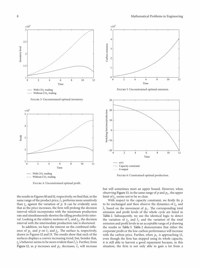built an EOQ model over a finite time horizon within adynamic control system The demand in the paper wasassumed to be uniformly distributed and set to depend on theprice over the replenishment period Differently Sana [2ndash5]assumed that the demand is display space as well as selling-price dependent within an EOQ system where the trade-offs between inventory costs purchasing costs the cost ofsales staff efforts and selling price were considered Bukhariand EI-Gohary [6] constructed an optimal control model ofproduction-maintenance system with deteriorating productsfor exploring the optimal production andmaintenance strate-gies within the schedule Shoude [7] extended EI-Goharyrsquosframework to a more general fashion in which the emissiontax and pollution RampD investment are considered as decisionvariables Early similar studies can be traced to Laffontand Tirole [8] in which the authors highlighted the impactof the existing and imminent carbon trading market onenterprisersquos strategies of pollution abatement and productionThe results state that the current emission trading marketis able to enhance the firmrsquos emission-reduction efforts butthe imminent completion mechanism will if known by thecompany weaken its enthusiasm of the pollution-abatementinvestment For this issue the authors from the perspectiveof mechanism design provided us with some measures andrecommendations on how to simultaneously analyze theuniversality of these proposalsThese papers essentially focuson the impact of external and internal emission reductionactivities on firmrsquos performances Caetano et al [9] presenteda study of the resourcemanagement on emission reduction byconstructing an optimal control model Although the paperdiscussed the dynamic relation between CO

2emission and

the reforestation investment and clean technology develop-ment it involves less production and operation Comparedwith the above literatures we do not either directly usethe EOQ framework or take any emission policies as thedecision variables but we contribute more on the studythat concerns the balance between the environmental andcommercial performances Besides according to many ofthe existing literatures this paper should be a forerunnerin synthetically modeling the relationship between emissioninventory and production among the researches of utilizing acontinuous optimal control on low-carbon issues Moreoverwe in this paper zoom in on some specific operation activitiesThe analysis and result are expected to be more constructivein conducting companyrsquos production and inventory man-agement Similar works include Dobosrsquos [10] in which theauthor took use of a concave production cost function indeveloping the firmrsquos optimal production strategy under thepolicies of carbon tax and emission standardThe studymadea comparison between the optimal solutions derived fromboth the original and modified versions from Arrow-Karlinrsquosresearch [11] Dobos [12ndash14] addressed a similar extension onthe classical A-K model by transforming the cost term into aconvex form In these studies the generation of carbon emis-sion is separately considered with production which ignoresthe relationship between emission and inventory processingHowever in practice among the companies such as HyundaiMotors Corporate a carbon footprint over the whole supplychain of motor manufacturing has to be considered Namely

the emission performance through the production process ofthemobile components needs to bemeasured andmonitored[15] In ourmodel the influences of production and inventoryprocessing on emission are synthetically simulated Namelywe abstracted the carbon footprint over a manufacturingsupply chain into two connected major operation activitiesthat is production and inventory processing In fact we findin the previous studies that while the modeling process doesreach the enterprise side the interest on the impact of the gov-ernment policies on the firmrsquos strategies is mainly discussedAccording to Gray and Shadbegian [16] pollution controland productive investment should be integrated although theformer will sometimes ldquocrowd outrdquo the latter on the empiricalstudy Chen and Monahan [17] analyzed the shortcomings ofemission standard policy claiming that people are paying toomuch attention to the validity of the policies compared to thereduction marginal cost For the other one even though wecan control the emission by the end of the planning horizonother kinds of pollution may be generated in advance duringthe production process An example is provided regarding theoveruse of raw materials excessive depletion of equipmentcaused by the production uncertainty as well as the riskbrought by stocking special merchandises Subramanian et al[18] addressed an analysis on firmrsquos gaming behavior againstthe emission reduction investment and trading strategieson production policies in carbon trading market under anauctioning mechanism The result shows that the impact ofdifferent quotas (that is more like the ldquocaprdquo of this paper) onhigh polluting industries is less than it functions on low typesBesides firmrsquos efforts on emission reduction will decrease asthe industrial pollution increases Furthermore the environ-mental protection activities may be able to provide a largerprofit to low polluting industries The author highlightedthe discussion on the interaction between firms rather thanputting interest on the operation details of the firm Gongand Zhou [19] employed a stochastic dynamic optimizationmodel to discuss companyrsquos multiperiod production strat-egy incorporating with the selection of clean or noncleanproduction technology under the cap-and-trade system Thefirm is modeled to decide whether to sell or purchase thequota at the end of each period which will sequentiallyinfluence the quota of the next cycle The emission volumeis assumed to be directly calculated by inventory level whichis positively affected by production The difference from ourpaper is that we only consider a single period but devotemoreinterests to the firmrsquos specific dynamic strategy rather thana binary decision-making problem The continuous modelwe used here is more adaptive in some particular industriessuch as the production of fluid or small particle productsCarmona et al [20] studied amulticompany decision-makingproblem in which the firms need to choose the clean ornonclean technology to optimally arrange their productionstrategies over a finite period Different from the paper inwhich the demand is assumed to be unelastic we in thecurrent research assume it to be dependent on inventorylevel For a single company Baker and Urban [21] foundthat customerrsquos consuming behavior will be affected by thesize of the displayed goods on shelves namely a higherinventory level of the retailers may generate a larger demand








411 Indices




42 Models


max int119879

0


(1)


Demand information


CO2CO2

Distribution


Supply




119868 (119905) = 119903 (119905) minus 119889 (119905) (2)



(119905) = 120572119903 (119905) + 120573119868 (119905) (3)





+ 1205822120572119903 (119905)

(4)




1= 1205821(120597119889

120597119868) minus 120573120582

2minus 119901(

120597119889

120597119868) +120597119888

120597119868 (5)




2= 0 (6)




120597119871

120597119903= minus120597119891

120597119903+ 1205821+ 1205721205822le 0 119903 ge 0 119903 (

120597119871

120597119903) = 0 (7)


1and 120582










2(120572119903 + 120573119868) (8)


1= 1205821120575 minus 120573120582

2+ ℎ minus 119901120575 (9)




120582lowast

1(119905) =


120575 (10)



119903lowast(119905) =


2120579120575 (11)

119868lowast(119905) = (

1

41205752120579) 119890minus(1+119879)120575

times ( (119890119905120575minus 1) (1 + 119890

119905120575minus 2119890119879120575) ℎ

+ (119890119905120575minus 1) 119901C ((1 + 119890

119905120575minus 2119890119879120575) 120573 minus 2119890

119879120575120572120575)

+120575 (41198901198791205751205751205791198680minus (119890119905120575minus 1) (1 + 119890

119905120575minus 2119890119879120575) 119901))

(11)1015840

119909lowast(119905)

= (1

41205753120579) 119890minus(119905+119879)120575


+ 120573 (1 minus 2119890119905120575+ 1198902119905120575minus 2119890119879120575+ 119890(119905+119879)120575

(2 minus 2119905120575)))

+ 119901C ( minus 2119890(119905+119879)120575

11990512057221205753

minus 2120572120573120575 (119890119905120575minus 1198902119905120575+ 119890119879120575

+119890(119905+119879)120575

(minus1 + 2119905120575))

+ 1205732(1 minus 2119890

119905120575+ 1198902119905120575minus 2119890119879120575

+119890(119905+119879)120575

(2 minus 2119905120575)))


+ 120573 (1 minus 2119890119905120575+ 1198902119905120575minus 2119890119879120575

+ 119890(119905+119879)120575

(2 minus 2119905120575)))

+ 4119890119879120575120575 ((119890119905120575minus 1) 120573119868

0+ 1198901199051205751205751199090) 120579))

(11)10158401015840



119901C but if 120572 gt (119890(119905minus119879)120575




119871 = minus1205791199032+ (1205821+ 1205822120572) 119903 + 120582

2120573119868 + 119901 (119872 + 120575119868) minus ℎ119868 minus 120582

1120575119868



119903lowast(119905) =

0 if 1205821+ 1205822120572 le 0

(1205821+ 1205822120572)

2120579if 0 le 120582

1+ 1205822120572 le 2120579119903max

119903max if 2120579119903max le 1205821 + 1205721205822

(13)





1(119905) = 119890

minus11990512057511986810in






119868lowast

1(119905) 119909lowast1(119905) and 119868











119862(ℎ minus 120575119901 + 120573119901

119862))])120575 See the proof





2will


120573119901119862lt minus120572120575119901



Appendix B


2will extend




3(119905) = 119890

minus11990512057511986830+ 119903max(1 minus 119890







3(119905) = (120575((1minus119890

minus119905120575)12057311986830+

12057511990930+ 119905(120573 + 119886120575)119903max) + (119890

minus119905120575minus 1)120573119903max)120575

2



3= log[119890119879120575(1 + 120575(120572119901

119862+ 2119903max120579)(ℎ minus 120575119901 +


follows Lemma 5





119862lt





2120597120572|ℎ+119901120573119888minus119901120575ltminus119901119888120572120575

lt


2or





3








119879 = 12 1198680= 1000 119901(119905) = 100 120572 = 2 120573 = 05 120575 = 02

120579 = 05 ℎ = 5 1199090= 500 119909 = 20000 119901C = 10 and

119903max = 20






2= 94459 Figure 7


0

20

40

60

80

Prod

uctio

n ra

te

0 2 4 6 8 10 12

Time

minus20






2is larger





0 2 4 6 8 10 12

Time

1

15

2

25

3

Inve

ntor

y le

vel


times104


0 2 4 6 8 10 12

Time

1

2

3

4

5


times105

Profi

t












0 2 4 6 8 10 12

Time

0

1

2

3

4

5

Carb

on em

issio

n

times105


0 2 4 6 8 10 12

Time

minus20

minus10

0

10

20

30

120590(t)


Switc

hing

func

tion

prod

uctio

n





2and



2and 119905





119901C 1199052

1199053



CO2 trading 119901 1199052

1199053


0 2 4 6 8 10 12

Time

minus20

0

20

40

60

Switc

hing

func

tion

prod

uctio

n

pC = 2

pC = 5

pC = 10



10 105 11 115 128

85

9

95

Switc

hing

tim

e for

0ou

tput

pC





10 105 11 115 12minus10

minus5

0

5

Switc

hing

tim

e for

mid

dle o

utpu

t

pC


9

95

10

105

11

Switc

hing

tim

e for

0ou

tput

100 110 120 130 140 150

p


100 110 120 130 140 150

p

2

4

6

8

10

Switc

hing

tim

e for

mid

dle o

utpu

t


100

120

140

160

p0

5

10

158

10

12

14

Switc

hing

tim

e for

0ou

tput

pC


100

120

140

160

p0

5

10

15minus5

0

5

10

15

Switc

hing

tim

e for

mid

dle o

utpu

t

pC





6 Conclusion







Appendices




119879120575minus



119879120575119901C(119890

119879120575minus 119890(1199051+Δ119905)120575) is also


1]



2isin [0 119879) is 120575120572119890119879120575119901C(119890


120575119890119879120575(2120579119903max + 120572119901C)(119890




120575120572119890119879120575119901C(119890



obtained


2on 119901 120597119905

2120597119901 =












119879120575(2120579119903max+120572119901C))(119890

119879120575minus119890119905120575) Evi-



3=

log[119890119879120575(1 + 120575(120572119901C + 2119903max120579)(ℎ minus 120575119901 + 120573119901C))]120575



Acknowledgments


References





































Volume 2014




Journal of











Journal of


Function Spaces






Algebra
















411 Indices




42 Models


max int119879

0


(1)


Demand information


CO2CO2

Distribution


Supply




119868 (119905) = 119903 (119905) minus 119889 (119905) (2)



(119905) = 120572119903 (119905) + 120573119868 (119905) (3)





+ 1205822120572119903 (119905)

(4)




1= 1205821(120597119889

120597119868) minus 120573120582

2minus 119901(

120597119889

120597119868) +120597119888

120597119868 (5)




2= 0 (6)




120597119871

120597119903= minus120597119891

120597119903+ 1205821+ 1205721205822le 0 119903 ge 0 119903 (

120597119871

120597119903) = 0 (7)


1and 120582










2(120572119903 + 120573119868) (8)


1= 1205821120575 minus 120573120582

2+ ℎ minus 119901120575 (9)




120582lowast

1(119905) =


120575 (10)



119903lowast(119905) =


2120579120575 (11)

119868lowast(119905) = (

1

41205752120579) 119890minus(1+119879)120575

times ( (119890119905120575minus 1) (1 + 119890

119905120575minus 2119890119879120575) ℎ

+ (119890119905120575minus 1) 119901C ((1 + 119890

119905120575minus 2119890119879120575) 120573 minus 2119890

119879120575120572120575)

+120575 (41198901198791205751205751205791198680minus (119890119905120575minus 1) (1 + 119890

119905120575minus 2119890119879120575) 119901))

(11)1015840

119909lowast(119905)

= (1

41205753120579) 119890minus(119905+119879)120575


+ 120573 (1 minus 2119890119905120575+ 1198902119905120575minus 2119890119879120575+ 119890(119905+119879)120575

(2 minus 2119905120575)))

+ 119901C ( minus 2119890(119905+119879)120575

11990512057221205753

minus 2120572120573120575 (119890119905120575minus 1198902119905120575+ 119890119879120575

+119890(119905+119879)120575

(minus1 + 2119905120575))

+ 1205732(1 minus 2119890

119905120575+ 1198902119905120575minus 2119890119879120575

+119890(119905+119879)120575

(2 minus 2119905120575)))


+ 120573 (1 minus 2119890119905120575+ 1198902119905120575minus 2119890119879120575

+ 119890(119905+119879)120575

(2 minus 2119905120575)))

+ 4119890119879120575120575 ((119890119905120575minus 1) 120573119868

0+ 1198901199051205751205751199090) 120579))

(11)10158401015840



119901C but if 120572 gt (119890(119905minus119879)120575




119871 = minus1205791199032+ (1205821+ 1205822120572) 119903 + 120582

2120573119868 + 119901 (119872 + 120575119868) minus ℎ119868 minus 120582

1120575119868



119903lowast(119905) =

0 if 1205821+ 1205822120572 le 0

(1205821+ 1205822120572)

2120579if 0 le 120582

1+ 1205822120572 le 2120579119903max

119903max if 2120579119903max le 1205821 + 1205721205822

(13)





1(119905) = 119890

minus11990512057511986810in






119868lowast

1(119905) 119909lowast1(119905) and 119868











119862(ℎ minus 120575119901 + 120573119901

119862))])120575 See the proof





2will


120573119901119862lt minus120572120575119901



Appendix B


2will extend




3(119905) = 119890

minus11990512057511986830+ 119903max(1 minus 119890







3(119905) = (120575((1minus119890

minus119905120575)12057311986830+

12057511990930+ 119905(120573 + 119886120575)119903max) + (119890

minus119905120575minus 1)120573119903max)120575

2



3= log[119890119879120575(1 + 120575(120572119901

119862+ 2119903max120579)(ℎ minus 120575119901 +


follows Lemma 5





119862lt





2120597120572|ℎ+119901120573119888minus119901120575ltminus119901119888120572120575

lt


2or





3








119879 = 12 1198680= 1000 119901(119905) = 100 120572 = 2 120573 = 05 120575 = 02

120579 = 05 ℎ = 5 1199090= 500 119909 = 20000 119901C = 10 and

119903max = 20






2= 94459 Figure 7


0

20

40

60

80

Prod

uctio

n ra

te

0 2 4 6 8 10 12

Time

minus20






2is larger





0 2 4 6 8 10 12

Time

1

15

2

25

3

Inve

ntor

y le

vel


times104


0 2 4 6 8 10 12

Time

1

2

3

4

5


times105

Profi

t












0 2 4 6 8 10 12

Time

0

1

2

3

4

5

Carb

on em

issio

n

times105


0 2 4 6 8 10 12

Time

minus20

minus10

0

10

20

30

120590(t)


Switc

hing

func

tion

prod

uctio

n





2and



2and 119905





119901C 1199052

1199053



CO2 trading 119901 1199052

1199053


0 2 4 6 8 10 12

Time

minus20

0

20

40

60

Switc

hing

func

tion

prod

uctio

n

pC = 2

pC = 5

pC = 10



10 105 11 115 128

85

9

95

Switc

hing

tim

e for

0ou

tput

pC





10 105 11 115 12minus10

minus5

0

5

Switc

hing

tim

e for

mid

dle o

utpu

t

pC


9

95

10

105

11

Switc

hing

tim

e for

0ou

tput

100 110 120 130 140 150

p


100 110 120 130 140 150

p

2

4

6

8

10

Switc

hing

tim

e for

mid

dle o

utpu

t


100

120

140

160

p0

5

10

158

10

12

14

Switc

hing

tim

e for

0ou

tput

pC


100

120

140

160

p0

5

10

15minus5

0

5

10

15

Switc

hing

tim

e for

mid

dle o

utpu

t

pC





6 Conclusion







Appendices




119879120575minus



119879120575119901C(119890

119879120575minus 119890(1199051+Δ119905)120575) is also


1]



2isin [0 119879) is 120575120572119890119879120575119901C(119890


120575119890119879120575(2120579119903max + 120572119901C)(119890




120575120572119890119879120575119901C(119890



obtained


2on 119901 120597119905

2120597119901 =












119879120575(2120579119903max+120572119901C))(119890

119879120575minus119890119905120575) Evi-



3=

log[119890119879120575(1 + 120575(120572119901C + 2119903max120579)(ℎ minus 120575119901 + 120573119901C))]120575



Acknowledgments


References





































Volume 2014




Journal of











Journal of


Function Spaces






Algebra










Demand information


CO2CO2

Distribution


Supply




119868 (119905) = 119903 (119905) minus 119889 (119905) (2)



(119905) = 120572119903 (119905) + 120573119868 (119905) (3)





+ 1205822120572119903 (119905)

(4)




1= 1205821(120597119889

120597119868) minus 120573120582

2minus 119901(

120597119889

120597119868) +120597119888

120597119868 (5)




2= 0 (6)




120597119871

120597119903= minus120597119891

120597119903+ 1205821+ 1205721205822le 0 119903 ge 0 119903 (

120597119871

120597119903) = 0 (7)


1and 120582










2(120572119903 + 120573119868) (8)


1= 1205821120575 minus 120573120582

2+ ℎ minus 119901120575 (9)




120582lowast

1(119905) =


120575 (10)



119903lowast(119905) =


2120579120575 (11)

119868lowast(119905) = (

1

41205752120579) 119890minus(1+119879)120575

times ( (119890119905120575minus 1) (1 + 119890

119905120575minus 2119890119879120575) ℎ

+ (119890119905120575minus 1) 119901C ((1 + 119890

119905120575minus 2119890119879120575) 120573 minus 2119890

119879120575120572120575)

+120575 (41198901198791205751205751205791198680minus (119890119905120575minus 1) (1 + 119890

119905120575minus 2119890119879120575) 119901))

(11)1015840

119909lowast(119905)

= (1

41205753120579) 119890minus(119905+119879)120575


+ 120573 (1 minus 2119890119905120575+ 1198902119905120575minus 2119890119879120575+ 119890(119905+119879)120575

(2 minus 2119905120575)))

+ 119901C ( minus 2119890(119905+119879)120575

11990512057221205753

minus 2120572120573120575 (119890119905120575minus 1198902119905120575+ 119890119879120575

+119890(119905+119879)120575

(minus1 + 2119905120575))

+ 1205732(1 minus 2119890

119905120575+ 1198902119905120575minus 2119890119879120575

+119890(119905+119879)120575

(2 minus 2119905120575)))


+ 120573 (1 minus 2119890119905120575+ 1198902119905120575minus 2119890119879120575

+ 119890(119905+119879)120575

(2 minus 2119905120575)))

+ 4119890119879120575120575 ((119890119905120575minus 1) 120573119868

0+ 1198901199051205751205751199090) 120579))

(11)10158401015840



119901C but if 120572 gt (119890(119905minus119879)120575




119871 = minus1205791199032+ (1205821+ 1205822120572) 119903 + 120582

2120573119868 + 119901 (119872 + 120575119868) minus ℎ119868 minus 120582

1120575119868



119903lowast(119905) =

0 if 1205821+ 1205822120572 le 0

(1205821+ 1205822120572)

2120579if 0 le 120582

1+ 1205822120572 le 2120579119903max

119903max if 2120579119903max le 1205821 + 1205721205822

(13)





1(119905) = 119890

minus11990512057511986810in






119868lowast

1(119905) 119909lowast1(119905) and 119868











119862(ℎ minus 120575119901 + 120573119901

119862))])120575 See the proof





2will


120573119901119862lt minus120572120575119901



Appendix B


2will extend




3(119905) = 119890

minus11990512057511986830+ 119903max(1 minus 119890







3(119905) = (120575((1minus119890

minus119905120575)12057311986830+

12057511990930+ 119905(120573 + 119886120575)119903max) + (119890

minus119905120575minus 1)120573119903max)120575

2



3= log[119890119879120575(1 + 120575(120572119901

119862+ 2119903max120579)(ℎ minus 120575119901 +


follows Lemma 5





119862lt





2120597120572|ℎ+119901120573119888minus119901120575ltminus119901119888120572120575

lt


2or





3








119879 = 12 1198680= 1000 119901(119905) = 100 120572 = 2 120573 = 05 120575 = 02

120579 = 05 ℎ = 5 1199090= 500 119909 = 20000 119901C = 10 and

119903max = 20






2= 94459 Figure 7


0

20

40

60

80

Prod

uctio

n ra

te

0 2 4 6 8 10 12

Time

minus20






2is larger





0 2 4 6 8 10 12

Time

1

15

2

25

3

Inve

ntor

y le

vel


times104


0 2 4 6 8 10 12

Time

1

2

3

4

5


times105

Profi

t












0 2 4 6 8 10 12

Time

0

1

2

3

4

5

Carb

on em

issio

n

times105


0 2 4 6 8 10 12

Time

minus20

minus10

0

10

20

30

120590(t)


Switc

hing

func

tion

prod

uctio

n





2and



2and 119905





119901C 1199052

1199053



CO2 trading 119901 1199052

1199053


0 2 4 6 8 10 12

Time

minus20

0

20

40

60

Switc

hing

func

tion

prod

uctio

n

pC = 2

pC = 5

pC = 10



10 105 11 115 128

85

9

95

Switc

hing

tim

e for

0ou

tput

pC





10 105 11 115 12minus10

minus5

0

5

Switc

hing

tim

e for

mid

dle o

utpu

t

pC


9

95

10

105

11

Switc

hing

tim

e for

0ou

tput

100 110 120 130 140 150

p


100 110 120 130 140 150

p

2

4

6

8

10

Switc

hing

tim

e for

mid

dle o

utpu

t


100

120

140

160

p0

5

10

158

10

12

14

Switc

hing

tim

e for

0ou

tput

pC


100

120

140

160

p0

5

10

15minus5

0

5

10

15

Switc

hing

tim

e for

mid

dle o

utpu

t

pC





6 Conclusion







Appendices




119879120575minus



119879120575119901C(119890

119879120575minus 119890(1199051+Δ119905)120575) is also


1]



2isin [0 119879) is 120575120572119890119879120575119901C(119890


120575119890119879120575(2120579119903max + 120572119901C)(119890




120575120572119890119879120575119901C(119890



obtained


2on 119901 120597119905

2120597119901 =












119879120575(2120579119903max+120572119901C))(119890

119879120575minus119890119905120575) Evi-



3=

log[119890119879120575(1 + 120575(120572119901C + 2119903max120579)(ℎ minus 120575119901 + 120573119901C))]120575



Acknowledgments


References





































Volume 2014




Journal of











Journal of


Function Spaces






Algebra
















2(120572119903 + 120573119868) (8)


1= 1205821120575 minus 120573120582

2+ ℎ minus 119901120575 (9)




120582lowast

1(119905) =


120575 (10)



119903lowast(119905) =


2120579120575 (11)

119868lowast(119905) = (

1

41205752120579) 119890minus(1+119879)120575

times ( (119890119905120575minus 1) (1 + 119890

119905120575minus 2119890119879120575) ℎ

+ (119890119905120575minus 1) 119901C ((1 + 119890

119905120575minus 2119890119879120575) 120573 minus 2119890

119879120575120572120575)

+120575 (41198901198791205751205751205791198680minus (119890119905120575minus 1) (1 + 119890

119905120575minus 2119890119879120575) 119901))

(11)1015840

119909lowast(119905)

= (1

41205753120579) 119890minus(119905+119879)120575


+ 120573 (1 minus 2119890119905120575+ 1198902119905120575minus 2119890119879120575+ 119890(119905+119879)120575

(2 minus 2119905120575)))

+ 119901C ( minus 2119890(119905+119879)120575

11990512057221205753

minus 2120572120573120575 (119890119905120575minus 1198902119905120575+ 119890119879120575

+119890(119905+119879)120575

(minus1 + 2119905120575))

+ 1205732(1 minus 2119890

119905120575+ 1198902119905120575minus 2119890119879120575

+119890(119905+119879)120575

(2 minus 2119905120575)))


+ 120573 (1 minus 2119890119905120575+ 1198902119905120575minus 2119890119879120575

+ 119890(119905+119879)120575

(2 minus 2119905120575)))

+ 4119890119879120575120575 ((119890119905120575minus 1) 120573119868

0+ 1198901199051205751205751199090) 120579))

(11)10158401015840



119901C but if 120572 gt (119890(119905minus119879)120575




119871 = minus1205791199032+ (1205821+ 1205822120572) 119903 + 120582

2120573119868 + 119901 (119872 + 120575119868) minus ℎ119868 minus 120582

1120575119868



119903lowast(119905) =

0 if 1205821+ 1205822120572 le 0

(1205821+ 1205822120572)

2120579if 0 le 120582

1+ 1205822120572 le 2120579119903max

119903max if 2120579119903max le 1205821 + 1205721205822

(13)





1(119905) = 119890

minus11990512057511986810in






119868lowast

1(119905) 119909lowast1(119905) and 119868











119862(ℎ minus 120575119901 + 120573119901

119862))])120575 See the proof





2will


120573119901119862lt minus120572120575119901



Appendix B


2will extend




3(119905) = 119890

minus11990512057511986830+ 119903max(1 minus 119890







3(119905) = (120575((1minus119890

minus119905120575)12057311986830+

12057511990930+ 119905(120573 + 119886120575)119903max) + (119890

minus119905120575minus 1)120573119903max)120575

2



3= log[119890119879120575(1 + 120575(120572119901

119862+ 2119903max120579)(ℎ minus 120575119901 +


follows Lemma 5





119862lt





2120597120572|ℎ+119901120573119888minus119901120575ltminus119901119888120572120575

lt


2or





3








119879 = 12 1198680= 1000 119901(119905) = 100 120572 = 2 120573 = 05 120575 = 02

120579 = 05 ℎ = 5 1199090= 500 119909 = 20000 119901C = 10 and

119903max = 20






2= 94459 Figure 7


0

20

40

60

80

Prod

uctio

n ra

te

0 2 4 6 8 10 12

Time

minus20






2is larger





0 2 4 6 8 10 12

Time

1

15

2

25

3

Inve

ntor

y le

vel


times104


0 2 4 6 8 10 12

Time

1

2

3

4

5


times105

Profi

t












0 2 4 6 8 10 12

Time

0

1

2

3

4

5

Carb

on em

issio

n

times105


0 2 4 6 8 10 12

Time

minus20

minus10

0

10

20

30

120590(t)


Switc

hing

func

tion

prod

uctio

n





2and



2and 119905





119901C 1199052

1199053



CO2 trading 119901 1199052

1199053


0 2 4 6 8 10 12

Time

minus20

0

20

40

60

Switc

hing

func

tion

prod

uctio

n

pC = 2

pC = 5

pC = 10



10 105 11 115 128

85

9

95

Switc

hing

tim

e for

0ou

tput

pC





10 105 11 115 12minus10

minus5

0

5

Switc

hing

tim

e for

mid

dle o

utpu

t

pC


9

95

10

105

11

Switc

hing

tim

e for

0ou

tput

100 110 120 130 140 150

p


100 110 120 130 140 150

p

2

4

6

8

10

Switc

hing

tim

e for

mid

dle o

utpu

t


100

120

140

160

p0

5

10

158

10

12

14

Switc

hing

tim

e for

0ou

tput

pC


100

120

140

160

p0

5

10

15minus5

0

5

10

15

Switc

hing

tim

e for

mid

dle o

utpu

t

pC





6 Conclusion







Appendices




119879120575minus



119879120575119901C(119890

119879120575minus 119890(1199051+Δ119905)120575) is also


1]



2isin [0 119879) is 120575120572119890119879120575119901C(119890


120575119890119879120575(2120579119903max + 120572119901C)(119890




120575120572119890119879120575119901C(119890



obtained


2on 119901 120597119905

2120597119901 =












119879120575(2120579119903max+120572119901C))(119890

119879120575minus119890119905120575) Evi-



3=

log[119890119879120575(1 + 120575(120572119901C + 2119903max120579)(ℎ minus 120575119901 + 120573119901C))]120575



Acknowledgments


References





































Volume 2014




Journal of











Journal of


Function Spaces






Algebra













1(119905) = 119890

minus11990512057511986810in






119868lowast

1(119905) 119909lowast1(119905) and 119868











119862(ℎ minus 120575119901 + 120573119901

119862))])120575 See the proof





2will


120573119901119862lt minus120572120575119901



Appendix B


2will extend




3(119905) = 119890

minus11990512057511986830+ 119903max(1 minus 119890







3(119905) = (120575((1minus119890

minus119905120575)12057311986830+

12057511990930+ 119905(120573 + 119886120575)119903max) + (119890

minus119905120575minus 1)120573119903max)120575

2



3= log[119890119879120575(1 + 120575(120572119901

119862+ 2119903max120579)(ℎ minus 120575119901 +


follows Lemma 5





119862lt





2120597120572|ℎ+119901120573119888minus119901120575ltminus119901119888120572120575

lt


2or





3








119879 = 12 1198680= 1000 119901(119905) = 100 120572 = 2 120573 = 05 120575 = 02

120579 = 05 ℎ = 5 1199090= 500 119909 = 20000 119901C = 10 and

119903max = 20






2= 94459 Figure 7


0

20

40

60

80

Prod

uctio

n ra

te

0 2 4 6 8 10 12

Time

minus20






2is larger





0 2 4 6 8 10 12

Time

1

15

2

25

3

Inve

ntor

y le

vel


times104


0 2 4 6 8 10 12

Time

1

2

3

4

5


times105

Profi

t












0 2 4 6 8 10 12

Time

0

1

2

3

4

5

Carb

on em

issio

n

times105


0 2 4 6 8 10 12

Time

minus20

minus10

0

10

20

30

120590(t)


Switc

hing

func

tion

prod

uctio

n





2and



2and 119905





119901C 1199052

1199053



CO2 trading 119901 1199052

1199053


0 2 4 6 8 10 12

Time

minus20

0

20

40

60

Switc

hing

func

tion

prod

uctio

n

pC = 2

pC = 5

pC = 10



10 105 11 115 128

85

9

95

Switc

hing

tim

e for

0ou

tput

pC





10 105 11 115 12minus10

minus5

0

5

Switc

hing

tim

e for

mid

dle o

utpu

t

pC


9

95

10

105

11

Switc

hing

tim

e for

0ou

tput

100 110 120 130 140 150

p


100 110 120 130 140 150

p

2

4

6

8

10

Switc

hing

tim

e for

mid

dle o

utpu

t


100

120

140

160

p0

5

10

158

10

12

14

Switc

hing

tim

e for

0ou

tput

pC


100

120

140

160

p0

5

10

15minus5

0

5

10

15

Switc

hing

tim

e for

mid

dle o

utpu

t

pC





6 Conclusion







Appendices




119879120575minus



119879120575119901C(119890

119879120575minus 119890(1199051+Δ119905)120575) is also


1]



2isin [0 119879) is 120575120572119890119879120575119901C(119890


120575119890119879120575(2120579119903max + 120572119901C)(119890




120575120572119890119879120575119901C(119890



obtained


2on 119901 120597119905

2120597119901 =












119879120575(2120579119903max+120572119901C))(119890

119879120575minus119890119905120575) Evi-



3=

log[119890119879120575(1 + 120575(120572119901C + 2119903max120579)(ℎ minus 120575119901 + 120573119901C))]120575



Acknowledgments


References





































Volume 2014




Journal of











Journal of


Function Spaces






Algebra













3








119879 = 12 1198680= 1000 119901(119905) = 100 120572 = 2 120573 = 05 120575 = 02

120579 = 05 ℎ = 5 1199090= 500 119909 = 20000 119901C = 10 and

119903max = 20






2= 94459 Figure 7


0

20

40

60

80

Prod

uctio

n ra

te

0 2 4 6 8 10 12

Time

minus20






2is larger





0 2 4 6 8 10 12

Time

1

15

2

25

3

Inve

ntor

y le

vel


times104


0 2 4 6 8 10 12

Time

1

2

3

4

5


times105

Profi

t












0 2 4 6 8 10 12

Time

0

1

2

3

4

5

Carb

on em

issio

n

times105


0 2 4 6 8 10 12

Time

minus20

minus10

0

10

20

30

120590(t)


Switc

hing

func

tion

prod

uctio

n





2and



2and 119905





119901C 1199052

1199053



CO2 trading 119901 1199052

1199053


0 2 4 6 8 10 12

Time

minus20

0

20

40

60

Switc

hing

func

tion

prod

uctio

n

pC = 2

pC = 5

pC = 10



10 105 11 115 128

85

9

95

Switc

hing

tim

e for

0ou

tput

pC





10 105 11 115 12minus10

minus5

0

5

Switc

hing

tim

e for

mid

dle o

utpu

t

pC


9

95

10

105

11

Switc

hing

tim

e for

0ou

tput

100 110 120 130 140 150

p


100 110 120 130 140 150

p

2

4

6

8

10

Switc

hing

tim

e for

mid

dle o

utpu

t


100

120

140

160

p0

5

10

158

10

12

14

Switc

hing

tim

e for

0ou

tput

pC


100

120

140

160

p0

5

10

15minus5

0

5

10

15

Switc

hing

tim

e for

mid

dle o

utpu

t

pC





6 Conclusion







Appendices




119879120575minus



119879120575119901C(119890

119879120575minus 119890(1199051+Δ119905)120575) is also


1]



2isin [0 119879) is 120575120572119890119879120575119901C(119890


120575119890119879120575(2120579119903max + 120572119901C)(119890




120575120572119890119879120575119901C(119890



obtained


2on 119901 120597119905

2120597119901 =












119879120575(2120579119903max+120572119901C))(119890

119879120575minus119890119905120575) Evi-



3=

log[119890119879120575(1 + 120575(120572119901C + 2119903max120579)(ℎ minus 120575119901 + 120573119901C))]120575



Acknowledgments


References





































Volume 2014




Journal of











Journal of


Function Spaces






Algebra










0 2 4 6 8 10 12

Time

1

15

2

25

3

Inve

ntor

y le

vel


times104


0 2 4 6 8 10 12

Time

1

2

3

4

5


times105

Profi

t












0 2 4 6 8 10 12

Time

0

1

2

3

4

5

Carb

on em

issio

n

times105


0 2 4 6 8 10 12

Time

minus20

minus10

0

10

20

30

120590(t)


Switc

hing

func

tion

prod

uctio

n





2and



2and 119905





119901C 1199052

1199053



CO2 trading 119901 1199052

1199053


0 2 4 6 8 10 12

Time

minus20

0

20

40

60

Switc

hing

func

tion

prod

uctio

n

pC = 2

pC = 5

pC = 10



10 105 11 115 128

85

9

95

Switc

hing

tim

e for

0ou

tput

pC





10 105 11 115 12minus10

minus5

0

5

Switc

hing

tim

e for

mid

dle o

utpu

t

pC


9

95

10

105

11

Switc

hing

tim

e for

0ou

tput

100 110 120 130 140 150

p


100 110 120 130 140 150

p

2

4

6

8

10

Switc

hing

tim

e for

mid

dle o

utpu

t


100

120

140

160

p0

5

10

158

10

12

14

Switc

hing

tim

e for

0ou

tput

pC


100

120

140

160

p0

5

10

15minus5

0

5

10

15

Switc

hing

tim

e for

mid

dle o

utpu

t

pC





6 Conclusion







Appendices




119879120575minus



119879120575119901C(119890

119879120575minus 119890(1199051+Δ119905)120575) is also


1]



2isin [0 119879) is 120575120572119890119879120575119901C(119890


120575119890119879120575(2120579119903max + 120572119901C)(119890




120575120572119890119879120575119901C(119890



obtained


2on 119901 120597119905

2120597119901 =












119879120575(2120579119903max+120572119901C))(119890

119879120575minus119890119905120575) Evi-



3=

log[119890119879120575(1 + 120575(120572119901C + 2119903max120579)(ℎ minus 120575119901 + 120573119901C))]120575



Acknowledgments


References





































Volume 2014




Journal of











Journal of


Function Spaces






Algebra











119901C 1199052

1199053



CO2 trading 119901 1199052

1199053


0 2 4 6 8 10 12

Time

minus20

0

20

40

60

Switc

hing

func

tion

prod

uctio

n

pC = 2

pC = 5

pC = 10



10 105 11 115 128

85

9

95

Switc

hing

tim

e for

0ou

tput

pC





10 105 11 115 12minus10

minus5

0

5

Switc

hing

tim

e for

mid

dle o

utpu

t

pC


9

95

10

105

11

Switc

hing

tim

e for

0ou

tput

100 110 120 130 140 150

p


100 110 120 130 140 150

p

2

4

6

8

10

Switc

hing

tim

e for

mid

dle o

utpu

t


100

120

140

160

p0

5

10

158

10

12

14

Switc

hing

tim

e for

0ou

tput

pC


100

120

140

160

p0

5

10

15minus5

0

5

10

15

Switc

hing

tim

e for

mid

dle o

utpu

t

pC





6 Conclusion







Appendices




119879120575minus



119879120575119901C(119890

119879120575minus 119890(1199051+Δ119905)120575) is also


1]



2isin [0 119879) is 120575120572119890119879120575119901C(119890


120575119890119879120575(2120579119903max + 120572119901C)(119890




120575120572119890119879120575119901C(119890



obtained


2on 119901 120597119905

2120597119901 =












119879120575(2120579119903max+120572119901C))(119890

119879120575minus119890119905120575) Evi-



3=

log[119890119879120575(1 + 120575(120572119901C + 2119903max120579)(ℎ minus 120575119901 + 120573119901C))]120575



Acknowledgments


References





































Volume 2014




Journal of











Journal of


Function Spaces






Algebra










10 105 11 115 12minus10

minus5

0

5

Switc

hing

tim

e for

mid

dle o

utpu

t

pC


9

95

10

105

11

Switc

hing

tim

e for

0ou

tput

100 110 120 130 140 150

p


100 110 120 130 140 150

p

2

4

6

8

10

Switc

hing

tim

e for

mid

dle o

utpu

t


100

120

140

160

p0

5

10

158

10

12

14

Switc

hing

tim

e for

0ou

tput

pC


100

120

140

160

p0

5

10

15minus5

0

5

10

15

Switc

hing

tim

e for

mid

dle o

utpu

t

pC





6 Conclusion







Appendices




119879120575minus



119879120575119901C(119890

119879120575minus 119890(1199051+Δ119905)120575) is also


1]



2isin [0 119879) is 120575120572119890119879120575119901C(119890


120575119890119879120575(2120579119903max + 120572119901C)(119890




120575120572119890119879120575119901C(119890



obtained


2on 119901 120597119905

2120597119901 =












119879120575(2120579119903max+120572119901C))(119890

119879120575minus119890119905120575) Evi-



3=

log[119890119879120575(1 + 120575(120572119901C + 2119903max120579)(ℎ minus 120575119901 + 120573119901C))]120575



Acknowledgments


References





































Volume 2014




Journal of











Journal of


Function Spaces






Algebra











6 Conclusion







Appendices




119879120575minus



119879120575119901C(119890

119879120575minus 119890(1199051+Δ119905)120575) is also


1]



2isin [0 119879) is 120575120572119890119879120575119901C(119890


120575119890119879120575(2120579119903max + 120572119901C)(119890




120575120572119890119879120575119901C(119890



obtained


2on 119901 120597119905

2120597119901 =












119879120575(2120579119903max+120572119901C))(119890

119879120575minus119890119905120575) Evi-



3=

log[119890119879120575(1 + 120575(120572119901C + 2119903max120579)(ℎ minus 120575119901 + 120573119901C))]120575



Acknowledgments


References





































Volume 2014




Journal of











Journal of


Function Spaces






Algebra










Appendices




119879120575minus



119879120575119901C(119890

119879120575minus 119890(1199051+Δ119905)120575) is also


1]



2isin [0 119879) is 120575120572119890119879120575119901C(119890


120575119890119879120575(2120579119903max + 120572119901C)(119890




120575120572119890119879120575119901C(119890



obtained


2on 119901 120597119905

2120597119901 =












119879120575(2120579119903max+120572119901C))(119890

119879120575minus119890119905120575) Evi-



3=

log[119890119879120575(1 + 120575(120572119901C + 2119903max120579)(ℎ minus 120575119901 + 120573119901C))]120575



Acknowledgments


References





































Volume 2014




Journal of











Journal of


Function Spaces






Algebra































Volume 2014




Journal of











Journal of


Function Spaces






Algebra









research article dynamic optimal production strategies based on...

Documents