optimal dynamic buffer management using optimal …jianghai/publication/tr-ece-07-18.pdfoptimal...
TRANSCRIPT

1
Optimal Dynamic Buffer Management Using Optimal Control
of Hybrid Systems
Wei Zhang and Jianghai Hu
School of Electrical and Computer Engineering
Purdue University, West Lafayette, IN 47907, USA.
zhang70, [email protected]
Abstract
This paper studies a dynamic buffer management problem withone buffer inserted between two
interacting components. The component to be controlled is assumed to have multiple power modes
corresponding to different data processing rates. The overall system is modeled as a hybrid system and the
buffer management problem is formulated as an optimal control problem. Different from many previous
studies, the objective function of the proposed problem depends on the switching cost and the size of
the continuous state space, making its solutions much more challenging. By exploiting some particular
features of the problem, the best mode sequence and the optimal switching instants are characterized
analytically using some variational approach. Simulationresult based on real data shows that the proposed
method can significantly reduce the energy consumptions compared with another heuristic scheme in
several typical situations.
I. INTRODUCTION
Dynamic buffer management (DBM) is an effective power management technique that can reduce the
power consumptions of electronic devices by inserting buffers among interacting components. The buffer
insertion makes it possible to turn off underutilized component at appropriate times without affecting
the service for the other components, thus reducing the system power consumption. The optimal buffer
size resulting in the largest power reduction is derived in [1], [2], [3] for some simple DBM problems.
A major limitation of these studies is that they all assume that the components to be controlled have
only two power modes, “on” and “off”. However, in practice, many components can work in more than
two power modes, such as the variable speed processors ([4])and the multi-speed disks ([5]). For such
a component, instead of completely turning it off, one can properly design a switching strategy, namely
the scheduling of different power modes of the component, tofurther reduce its power consumption.

2
This paper studies a more general DBM problem, where the component to be controlled has multiple
power modes. Since different power modes correspond to different data accumulation/depletion rates
in the buffer, the overall system is perfectly modeled as a piecewise-constant hybrid system, or more
accurately, a multi-rate automata ([6]). The DBM problem isthus formulated as an optimal control
problem of the underlying hybrid system.
Optimal control of hybrid systems is a challenging researchtopic that has attracted many researchers.
In [7], a unified framework is formulated for optimal controlof hybrid systems; some conceptual
algorithms based on the Bellman equation are also proposed for computing the optimal control policies.
A similar idea is employed in [8], where a more detailed algorithm based on the discretization of the
continuous state space is developed to solve the Bellman inequality. In [9], [10], a two-stage optimization
method is proposed for switched systems, where in the first stage the optimal continuous input is computed
for a fixed switching strategy and then in the second stage thedynamic programming algorithm is used
to compute the best switching strategy. In parallel with these dynamic-programming-based approaches,
variational methods have also been extensively studied. In[11], [12], the maximum principle is generalized
to solve a time optimal control and a linear quadratic control problem for switched systems with linear
subsystems. Some more general versions of the maximum principle for hybrid systems are proved in [13]
and [14]. Variational approaches are also used in [15], [16]to derive necessary conditions for the optimal
switching instants and/or the optimal continuous control input for switched systems with a fixed switching
sequence. Although an algorithm for updating the switchingsequence is discussed in [16], finding the
best switching sequence is still an NP-hard problem. More recently, [17] propose a way of embedding
a switched system into a larger family of systems, whose solutions, obtained by the traditional optimal
control methods, can be used to construct the optimal control of the switched systems without enumerating
the switching sequences. Besides these theoretical works,applications of the optimal control theory of
hybrid systems in various practical contexts have also beenwell studied. The problems in this category
as in [18], [19], [20], [21], usually deal with particular model structures and cost functions that often
enable one to find better analytical and numerical solutions. The optimal control problem considered in
this paper falls into this category.
Despite the richness of the literature in this field, the problem studied in this paper can not be directly
solved using the existing methods as it has the following distinct features: (i) transitions among discrete
modes depend on the evolution of the continuous state; whereas many previous studies ignore such
dependency; (ii) the switching (mode) sequence is a decision variable that cannot be assumed fixed; (iii)
the switching cost ignored in most previous papers is an important part of our cost function; (iv) the

3
2 2( , )r p
1 1( , )r p
( , )N Nr p
2r
X Y
yr
Buffer B
Fig. 1. System Configuration
buffer size that determines the range of the continuous states is variable, indicating that both the optimal
control and the optimal size of the continuous state space are to be designed at the same time. Few
existing results have addressed all of these issues.
The main contributions of this paper are the following: (i) Hybrid system framework is successfully
applied to model the DBM problem, which is an important problem in the low power design of embedded
systems. (ii) Two practically important DBM problems are formulated as optimal control problems of
a piecewise-constant hybrid system and solved analytically through a variational approach. (iii) Several
issues of implementing the proposed optimal strategy in practical systems are addressed. The results are
also verified through some simulations based on real data.
The rest of this paper is organized as follows. In Section II,two DBM problems are introduced and
formulated as optimal control problems of a piecewise constant hybrid system. In Section III, several
operations on hybrid trajectories are introduced. These operations are then used in Sections IV and V to
derive the optimal solutions. Two simulation examples are given in Section VI to illustrate the effectiveness
of the optimal strategies. Concluding remarks and future research directions are discussed in Section VII.
II. PROBLEM FORMULATION
A. System Description
Consider two interacting components X and Y as shown in Fig. 1, where X produces data for Y to
consume. Suppose that Y is always “on” and consumes data at a constant speedry. On the other hand,
assume that X hasN different operation modes where in modei, i = 1, 2, . . . , N , it produces data at a
constant speedri and consumes powerpi. Without loss of generality, assumer1 < r2 < · · · < rN . Usually,
a lower data rate corresponds to a lower power consumption; thus we requirep1 < p2 < · · · < pN . Denote
by I andJ the sets of indices whose corresponding data rates are greater and smaller thanry, respectively,

4
i.e.,
I = i | ri > ry, i = 1, . . . , N,
and J = j | rj < ry, j = 1, . . . , N.
Assume that bothI andJ are nonempty, i.e.,rN > ry > r1. Note that we ignore the degenerate case
where ry can be perfectly matched by one of the power modes of X, since in this case no buffer is
needed and the DBM problem becomes trivial. A modeσ is called anascending mode if σ ∈ I and a
descending mode otherwise. To ensure smooth operation, a buffer B with capacity Q is inserted between
X and Y. See Fig. 1 for the configuration of the overall system.
Many real-world applications can be described by the above system. One simple example is the data-
copying process, where a device Y copies data from a hard drive X. The hard drive has two power modes
“on” and “off”. If the data rate of the hard drive is faster than that of Y, then X can be turned off during
some time intervals to save energy. In this case, the system memory, which serves as the buffer B in our
model, is needed to temporarily store the data from X for later delivery. As another example, consider the
video playing process. Let X be the Intel Xscale processor ([22]) that can operate on multiple voltages
corresponding to different speedsri’s and powerspi’s; let Y be a video card that demands data from
X at a constant speed, say 30frame/sec. To ensure smooth operation, the system memory is needed as
a buffer to store the data that has been decoded by X but yet to be displayed by Y. Thus, the abstract
system as shown in Fig. 1 represents a class of practical systems. Minimizing the power consumption of
such a system has important practical implications.
B. Hybrid System Model
The above problem can be modeled as a hybrid system H. The discrete state space of H consists of
N modes:S = 1, 2, . . . , N, corresponding to the operation modes of X. The continuous state q(t) is
defined as the amount of data stored in the buffer B, and is thusrequired to take values in the interval
[0, Q]. The evolution ofq(t) is determined by the speed difference between the two components, i.e.,
q(t) = ri − ry for modei. As a physical constraint, there can be no buffer underflow oroverflow. Thus,
we require that wheneverq(t) hits the boundary of its domain, namely,q(t) = 0 or Q, the system must
transit to another mode that can bringq(t) back to the inside of[0, Q]. Except for this, there are no other
transition rules and guard conditions. The reset map of the system is trivial, i.e., there is no jump inq(t)
at the transition instant.

5
( )q t
Q
ft0
General Trajectory
(a)
0
Periodic Trajectory
(c)
……
T
( )q t
Q
0
Feasible Trajectory
(b) ft
0
Boundary Switching
Trajectory
(e) ft
( )q t
( )q t
1 1 , i j 2 2 , i j1 1 , i j
3i 3j
( )q t
Q
0
-Trajectory
(d) ft
i j
( )q t
Q
0
Pure Trajectory
(f) ft
, i j , i j , i j
Λ
Fig. 2. Hybrid trajectories
Given a time period[0, tf ], the behavior of the above system can be uniquely determinedby the
switching strategyσ : [0, tf ] → S, which determines the active mode of the system over[0, tf ]. The
overall trajectoryz(t) = (q(t), σ(t)) of the hybrid system consists of the trajectories of the continuous
stateq(t) and the discrete stateσ(t). For a given initial valueq(0), the system is governed by the following
differential equation:
dq(t)
dt= rσ(t) − ry, ∀t ∈ [0, tf ]. (1)
In this paper, we study the power consumption of the whole process of transferring a certain amount of
data from X to Y. It is thus required that the system must startwith an empty buffer att = 0 and end
up with an empty buffer att = tf when Y have received all the data produced by X. This yields two
boundary conditions for the continuous state, namely,q(0) = 0 and q(tf ) = 0. The hybrid trajectories
that satisfy these two conditions are calledfeasible trajectories (See Fig. 2-(b)).
Assume that there is a partition of[0, tf ], t0 = 0 ≤ t1 ≤ . . . ≤ tn = tf , for somen ≥ 0, so that
σ(t) ≡ σi ∈ S is constant in each subinterval[ti−1, ti), i = 1, . . . , n. The sequence(σ1, . . . , σn) is called

6
the switching sequence and (t0, . . . , tn−1) is called theswitching instants1.
A hybrid trajectoryz(t) = (q(t), σ(t)) over [0,∞) is calledperiodic with periodT if q(t + T ) = q(t)
andσ(t + T ) = σ(t) for all t ∈ [0,∞). For such a trajectory, denote bynT the number of switchings in
each period. For example,nT = 5 for the trajectory in Fig 2-(c).
A feasible trajectory is called aΛ-trajectory if it consists of one ascending modei and one descending
modej with exactly two switchings as shown in Fig 2-(d). The pair ofmodesi, j in a Λ-trajectory is
called aΛ-pair.
A feasible trajectoryz(t) = (q(t), σ(t)) with switching instants(t0, . . . , tn−1) is called aboundary-
switching trajectory (BST) if q(ti) = Q or 0 for any i = 0, . . . , n − 1. In other words, a BST only
switches at the boundary of the range ofq(t). Denote byΩ the class of all BST’s. Every BST can be
decomposed into a series ofΛ-trajectories with the same buffer size. Denote bynp the number ofdistinct
Λ-pairs in a BST. For example,np = 3 for the BST in Fig 2-(e). A BST is calledpure if np = 1 and is
calledmixed otherwise. In other words, a pure trajectory must be a BST andis obtained by repeating a
Λ-trajectory for a certain number of times (See Fig. 2-(f)).
The power consumption of a given hybrid trajectoryz(t) = (q(t), σ(t)) consists of three parts: the
running power, namely the power consumed by componentX2, theswitching power and thebuffer power.
Note thatpσ(t) is the instantaneous power of X at timet. Thus the average running power over[0, tf ]
is 1tf
∫ tf
0 pσ(t)dt. Assume that switchings among different modes consumes thesame amount of energy
ks3. Then the average switching power over[0, tf ] is nks/tf , wheren is the number of switchings in
the trajectoryz. The buffer power includes the static buffer power and the dynamic buffer power. The
static buffer power is proportional to the buffer size whilethe dynamic buffer power only depends on
the actual amount of data in the buffer. Since the dynamic buffer power is much smaller than the static
one, in this paper, we only consider the static buffer power and denote it bypbQ, wherepb is a positive
constant andQ is the buffer size. Thus the total average power of the systemduring [0, tf ] can be written
as
P (z;Q, tf ) =1
tf
∫ tf
0pσ(t)dt +
nks
tf+ pbQ, (2)
1The system is turned on att = 0. Hence, we assume that there is always a switching att = 0 and ignore the switching, if
any, att = tf for all trajectories.
2The power ofY is ignored in this paper since it is a constant independent ofthe switching strategy.
3There may exist other switching penalties, such as the switching delay penalty. To simplify discussion, we assume that all
the switching penalties are transformed to an equivalent energy cost and incorporated intoks.

7
and the total energy associated withz(t) during [0, tf ] is
Eσ(z;Q, tf ) =
∫ tf
0pσ(t)dt + nks + pbQ · tf .
The three terms on the right hand side of the above equation represent therunning energy, theswitching
energy, and thebuffer energy, respectively.
C. Problem Statements
The goal of this paper is to find a feasible trajectory that canfinish a given task with the least energy
consumption. For some applications, the amount of data to betransferred to Y is knowna priori. In this
case,tf is a given constant which equals to the amount of data to be transferred divided by the data rate
of Y. The energy minimization problem can be formulated as the following optimal control problem of
the hybrid system H.
Problem 1: minz,Q P (z;Q, tf ) subject to the constraints: (i)z(t) = (q(t), σ(t)) satisfies equation (1);
(ii) q(t) ∈ [0, Q], ∀t ∈ [0, tf ] andq(0) = q(tf ) = 0; (iii) σ(t) ∈ S, ∀t ∈ [0, tf ].
Problem 1 requires the exact knowledge oftf . However, in some applications, the time horizontf is
not knowna priori. For example, consider that a network card (component X) downloads a live video
broadcast from the internet and at the same time sends the received data to a video card (component
Y). The tf in this example may not be known until X receives the last frame. In this case, we are
usually interested in periodic strategies that are easy to implement and whose power can be computed
even without the knowledge oftf . Therefore, another meaningful problem is to find the optimal periodic
trajectory with the least average power consumption.
Let z(t) be a periodic trajectory with(σ1, . . . , σnT) and (t0, . . . , tnT−1) as the switching sequence
and switching instants during the first period[0, T ], respectively. Note that the periodic trajectory has an
infinite length, i.e.,tf = ∞. The average power ofz is the same as its average power during the first
period, i.e.,
P (z;Q,∞)= P (z;Q,T )=1
T
(nT∑
i=1
pσiτi+nTks
)
+pbQ,
whereτi = ti − ti−1. Since every feasible solution must start with zero buffer,it follows that q(T ) =
q(0) = 0. Different from Problem 1, to find the best periodic solution, one not only needs to optimize the
switching sequence and switching instants, but also needs to find the best periodT . This is formulated
as the following problem.
8
Problem 2: minz,Q,T P (z;Q,T ) subject to the constraints: (i)z(t) = (q(t), σ(t)) is periodic with
periodT and satisfies equation (1); (ii)q(t) ∈ [0, Q], ∀t ∈ [0, T ] and q(0) = q(T ) = 0; (iii) σ(t) ∈ S,
∀t ∈ [0, T ].
Remark 1: The two problems in this section are independent of each other and serve different purposes.
Problem 1 is suitable for the case where the value oftf is known exactly before the system starts operating.
On the other hand, for unknowntf , Problem 2 prepares for the worst case by assumingtf = ∞ and only
focuses on infinite-length periodic strategies. However, for real applications the time horizontf must be
finite. Thus, when the solution of Problem 2 is applied to a real system, only part of the strategy will be
used. See Section IV-C for implementation details of periodic strategies.
For any optimal solutions to Problem 1 and 2, to avoid the unnecessary power consumption by the
unused buffer space,Q should be chosen as small as possible so that the buffer is full at least once
during [0, tf ]. In addition, sinceq(t) ≥ 0 andq(0) = 0, the following lemma follows immediately.
Lemma 1: If z(t) = (q(t), σ(t)) is an optimal solution to Problem 1, then
mint∈[0,tf ]
q(t) = 0, and maxt∈[0,tf ]
q(t) = Q.
This condition also holds for Problem 2 withtf replaced byT .
According to Lemma 1, the optimal buffer size is completely determined by a given trajectoryz(t).
From now on, we will callQ a valid buffer size of z if max q(t) ≤ Q and theoptimal buffer size of z
if equality holds.
The rest of this paper is devoted to deriving analytical solutions to the two problems formulated in this
section. Specifically, we will prove that: (i) the optimal solutions to both problems must be boundary-
switching trajectories (BST’s); (ii) the optimal pure periodic trajectory (OPPT) withnp = 1 is an optimal
solution to Problem 2 for an arbitrarynp; (iii) the optimal pure trajectory (OPT) with lengthtf andnp = 1
is an optimal solution to Problem 1 for an arbitrarynp; (iv) the OPT is different from the OPPT in general
and will converge to the OPPT astf goes to infinity. Although we consider all feasible trajectories as
candidate solutions, the above results enable us to only focus on pure (periodic) trajectories in finding
the optimal solutions. Since a pure trajectory involves only one (distinct)Λ-pair and only switches when
q(t) is 0 or Q, the OPT and OPPT, which are optimal solutions to Problems 1 and 2, can be easily
characterized analytically.
III. O PERATIONS ONHYBRID TRAJECTORIES
In this section, we introduce some important operations that can transform an existing trajectory to
a new one while preserving certain properties. These operations play an important role in deriving the

9
optimal solutions to Problems 1 and 2.
A. Cropping
Cropping, denoted byCa,b[·], is an operation that obtains a new trajectory by trimming off the
uninteresting parts of the original trajectory. For example, the cropped trajectoryCa,b[z] will only keep
the part ofz(t) wheret ∈ [a, b], i.e.,
Ca,b[z](t) = z(t + a), for t ∈ [0, b − a].
B. Joining
Joining, denoted byJ [·, · · · , ·], is an operation that obtains a new trajectory by putting several
finite-length trajectories together. For example,J [z(1), z(2)] corresponds to a new trajectory obtained
by appendingz(2) to the end ofz(1). More precisely,
J [z(1), z(2)](t) =
z(1)(t) , t ∈ [0, t(1)f ]
z(2)(t − t(1)f ) , t ∈ [t
(1)f , t
(1)f + t
(2)f ]
,
wheret(1)f and t
(2)f are the lengths ofz(1) andz(2), respectively. To prevent introducing discontinuities,
it is required thatz(1) and z(2) have consistent boundary conditions, i.e.,q(1)(t(1)f ) = q(2)(0), where
q(1) and q(2) are the continuous states ofz(1) andz(2), respectively. Denote byJm[z] a special joining
operation that repeats the trajectoryz satisfyingz(0) = z(tf ) for m times, i.e.,
Jm[z] = J [z, . . . , z︸ ︷︷ ︸
m z′s
].
C. Periodic Extension
Periodic extension, denoted byP[·], is an operation that obtains a periodic trajectory by repeating a
given trajectoryz for infinitely many times. Mathematically,P[·] can be defined in terms of the joining
operation asP[z] = J∞[z]. For a trajectoryz(t) of length tf , P[z](t + l · tf ) = z(t) for all t ∈ [0, tf ]
and any nonnegative integerl .
D. Scaling
For an arbitrary hybrid trajectoryz(t) = (q(t), σ(t)), the scaling operation with parameterc > 0 is
defined as
Sc[z](t) = (cq(t/c), σ(t/c)).
10
Q
( )q t
0 ft
Q
( )q t
0 / 3ft
Q
( )q t
0 ft
3
Q
Step 1 Step 2 Step 3
(a) (b) (c)
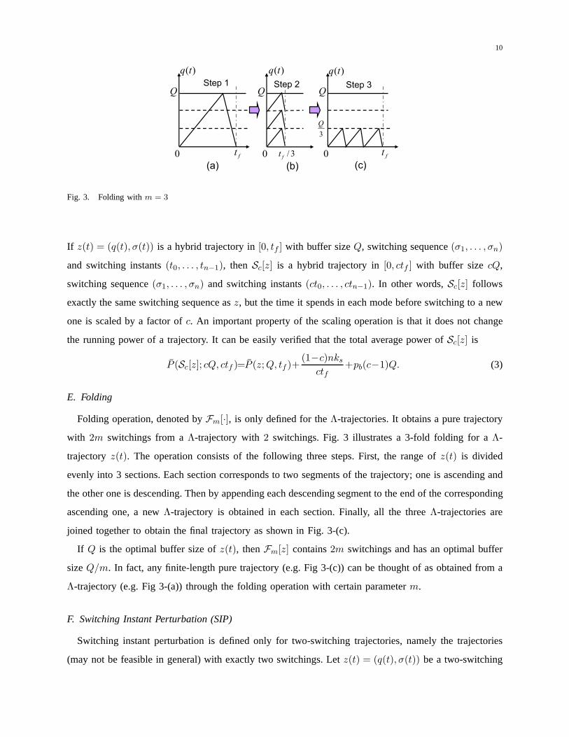
Fig. 3. Folding withm = 3
If z(t) = (q(t), σ(t)) is a hybrid trajectory in[0, tf ] with buffer sizeQ, switching sequence(σ1, . . . , σn)
and switching instants(t0, . . . , tn−1), thenSc[z] is a hybrid trajectory in[0, ctf ] with buffer sizecQ,
switching sequence(σ1, . . . , σn) and switching instants(ct0, . . . , ctn−1). In other words,Sc[z] follows
exactly the same switching sequence asz, but the time it spends in each mode before switching to a new
one is scaled by a factor ofc. An important property of the scaling operation is that it does not change
the running power of a trajectory. It can be easily verified that the total average power ofSc[z] is
P (Sc[z]; cQ, ctf )=P (z;Q, tf )+(1−c)nks
ctf+pb(c−1)Q. (3)
E. Folding
Folding operation, denoted byFm[·], is only defined for theΛ-trajectories. It obtains a pure trajectory
with 2m switchings from aΛ-trajectory with2 switchings. Fig. 3 illustrates a 3-fold folding for aΛ-
trajectory z(t). The operation consists of the following three steps. First, the range ofz(t) is divided
evenly into 3 sections. Each section corresponds to two segments of the trajectory; one is ascending and
the other one is descending. Then by appending each descending segment to the end of the corresponding
ascending one, a newΛ-trajectory is obtained in each section. Finally, all the three Λ-trajectories are
joined together to obtain the final trajectory as shown in Fig. 3-(c).
If Q is the optimal buffer size ofz(t), thenFm[z] contains2m switchings and has an optimal buffer
sizeQ/m. In fact, any finite-length pure trajectory (e.g. Fig 3-(c))can be thought of as obtained from a
Λ-trajectory (e.g. Fig 3-(a)) through the folding operationwith certain parameterm.
F. Switching Instant Perturbation (SIP)
Switching instant perturbation is defined only for two-switching trajectories, namely the trajectories
(may not be feasible in general) with exactly two switchings. Let z(t) = (q(t), σ(t)) be a two-switching

11
Q
( )q t
0ft
1q
2q
1t
Q
( )q t
0ft
1q
2q
1th
1 2
1
2
ˆft
( )z t[ ]( )h z t
Fig. 4. Switching instant perturbationHh[z] with h < t1
trajectory with switching sequence(σ1, σ2), switching instants(0, t1) and buffer sizeQ. Suppose that
q(0) = q1, q(tf ) = q2. Denote byHh[z] = (q(t), σ(t)) the SIP ofz. Roughly speaking, the SIP is
an operation that perturbs the switching instantt1 to a neighboring valueh while at the same time
changes the timetf accordingly to a certain valuetf to maintain the same trajectory boundary values,
i.e., q(0) = q1 and q(tf ) = q2. Fig. 4 illustrates an example of obtainingHh[z] from z(t). It can be seen
that the new trajectoryHh[z] switches from modeσ1 to modeσ2 at time h instead oft1 and ends at
time tf when its continuous state hitsq2. Mathematically, the perturbed trajectoryHh[z] = (q(t), σ(t))
can be defined as
σ(t) =
σ1 , t ≤ h
σ2 , h < t ≤ tf,
dq(t)
dt=rσ(t) − ry, for t ∈ [0, tf ],
and tf =h +h(ry − rσ1
) + q2 − q1
rσ2− ry
.
(4)
Under the above notations, a SIPHh[z] is calledvalid if
0 ≤ h ≤ tf and q(t) ∈ [0, Q] ∀t ∈ [0, tf ]. (5)
In other words,Hh[z] is valid if it spends nonnegative time in each mode and it doesnot cause any
buffer overflow or underflow. The set ofh for which Hh[z] is valid is called thedomain of h and is
denoted byDh. Thus for anyh ∈ Dh, z = Hh[z] defined in (4) satisfies the following properties:
1) z follows the same switching sequence(σ1, σ2) asz and spends nonnegative time in each mode.
2) q(0) = q(0) = q1 and q(tf ) = q(tf ) = q2.
3) q(t) ∈ [0, Q] for all t ∈ [0, tf ].
Note thatDh is a bounded connected interval. For example, consider the trajectoryz1 as shown in
Fig. 5-(a). Let(q(t), σ(t)) = Hh[z1](t). If h < a, then tf as defined in (4) will be less thanh, which

12
Q
( )q t
0ft
1q
2q
1t
1 2
1( )z t
hD
Q
( )q t
0 ft1q
2q
1t
1
2
2 ( )z t
hD
(a) (b)
a b c
Fig. 5. Range of SIP in two typical cases
violates the first condition in (5). On the other hand, ifh > b, thenq(t) < 0 for t ∈ (b, h], which violates
the second condition in (5). Hence,Dh = [a, b] for z1. As another example, consider the trajectoryz2
as shown in Fig. 5-(b) for whichq(t1) is on the boundary of[0, Q]. By a similar argument as in the
first example, the range ofh for z2 is Dh = [c, t1]. It is observed from these two examples that if
q(ti) ∈ (0, Q), thent1 is an interior point ofDh. On the other hand, ifq(ti) = 0 or Q, thenti is on the
boundary ofDh. This property actually holds for the SIP of arbitrary two-switching trajectories.
The SIP is a specific yet useful operation. Since it can perturb the switching instant without affecting
the boundary values (q(0) andq(tf )) and the buffer sizeQ, it can be used, together with other operations
such as cropping and joining, to study the effect of perturbing only one switching instant of a general
trajectory.
IV. OPTIMAL PERIODIC SOLUTION
In this section, we derive the optimal solutions of Problem 2(denoted by OS2 for simplicity). The
following lemma can greatly simplify the problem and is crucial for later proofs.
Lemma 2: If z is an OS2, thenz ∈ Ω. In other words, optimal solutions to Problem 2 must be
boundary-switching trajectories.
Proof: The key idea of the proof is to use the operations defined in Section III to construct a better
trajectory with less power consumption for any given trajectory that has switchings at some interior
points of [0, Q]. Let (z(t), Q, T ) be a solution to Problem 2. Denote by(σ1, . . . , σnT) and(t1, . . . , tnT
)
the switching sequence and switching instants in the first period of z(t). Suppose thatz(t) has a switching
at some interior point of[0, Q], i.e., 0 < q(ti) < Q for somei. Divide the first period ofz(t) into three

13
1E 3E
1it 1itit
( )q t
Q
t
1q
2q
i 1i
T
(1)z (2)z (3)z
(a) z(t) with switching at an interior point
1E 3E
1it 1itit t
i
1i
h
( )q t
Q
1q
2q
ThT
(1)z(2)
hz(3)z
(b) The perturbed trajectoryzh(t)
Fig. 6. Scheme of variation
parts through the cropping operation as shown in Fig. 6-(a):
z(1)(t) = C0,ti−1[z](t), z(2)(t) = Cti−1,ti+1
[z](t),
and z(3)(t) = Cti+1,T [z](t). (6)
Assume thatz(2)(t) = (q(2)(t), σ(2)(t)), q(2)(0) = q1 andq(2)(ti+1 − ti−1) = q2. Perform the SIP onz(2)
to obtain a new trajectoryz(2)h = (q
(2)h (t), σ
(2)h (t)) , Hh[z(2)]. According to (4), the length ofz(2)
h is
t(2)h = h +
h(ry − rσi) + q2 − q1
rσi+1 − ry. (7)
By definition, the SIP does not change the boundary values ofz(2), i.e., q(2)h (0) = q1 andq
(2)h (t
(2)h ) = q2.
Thus we can rejoinz(1), z(2)h andz(3) as shown in Fig. 6-(b) to obtain
zh , J [z(1), z(2)h , z(3)]. (8)
It is obvious that the length ofzh is
Th = ti−1 + t(2)h + (T − ti+1). (9)
Now we show thatzh consumes less power thanz for someh. Recall thatDh is the set ofh that z(2)h
remains valid. According to (5),Q is a valid buffer size forzh if h ∈ Dh. Thus∀h ∈ Dh the power of
14
1E 3E
1it 1itit t
i
1i
h
( )q t
Q
1q
2q
ThT
(2)
az(3)z(1)z
(a) Degenerate to no switching
1E 3E
1it 1itit t
i
1i
h
( )q t
Q
1q
2q
T hT
(2)
bz(3)z(1)z
(b) Switch at the boundary
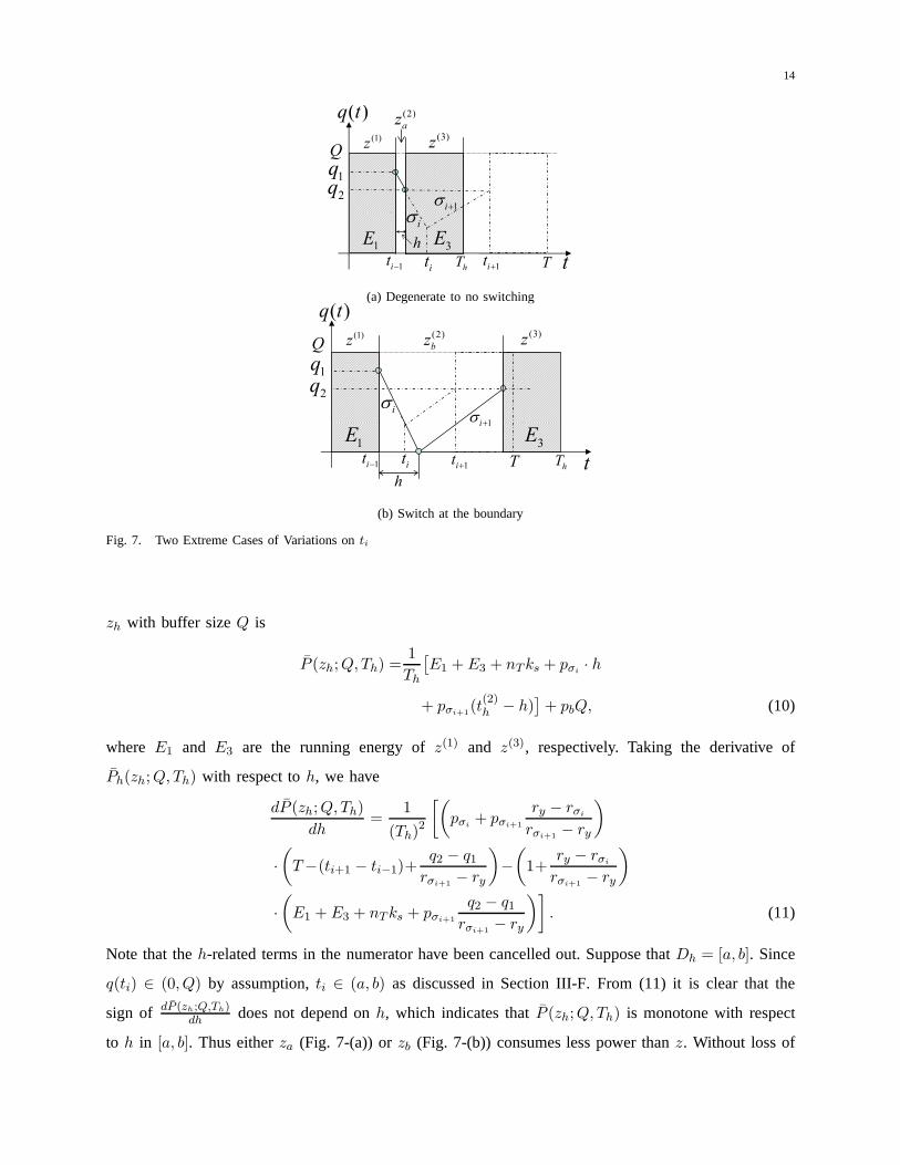
Fig. 7. Two Extreme Cases of Variations onti
zh with buffer sizeQ is
P (zh;Q,Th) =1
Th
[E1 + E3 + nTks + pσi
· h
+ pσi+1(t
(2)h − h)
]+ pbQ, (10)
where E1 and E3 are the running energy ofz(1) and z(3), respectively. Taking the derivative of
Ph(zh;Q,Th) with respect toh, we have
dP (zh;Q,Th)
dh=
1
(Th)2
[(
pσi+ pσi+1
ry − rσi
rσi+1− ry
)
·(
T−(ti+1 − ti−1)+q2 − q1
rσi+1− ry
)
−(
1+ry − rσi
rσi+1− ry
)
·(
E1 + E3 + nTks + pσi+1
q2 − q1
rσi+1− ry
)]
. (11)
Note that theh-related terms in the numerator have been cancelled out. Suppose thatDh = [a, b]. Since
q(ti) ∈ (0, Q) by assumption,ti ∈ (a, b) as discussed in Section III-F. From (11) it is clear that the
sign of dP (zh;Q,Th)dh does not depend onh, which indicates thatP (zh;Q,Th) is monotone with respect
to h in [a, b]. Thus eitherza (Fig. 7-(a)) orzb (Fig. 7-(b)) consumes less power thanz. Without loss of

15
generality, assumeza consumes less power thanz. Then the periodic extension ofza, P[za], is a better
periodic solution to Problem 2 thanz. Thus it follows thatq(ti) = 0 or Q for all i = 1, . . . , nT , i.e., the
OS2 must be a BST.
Lemma 2 enables one to focus on the BST’s (Ω) in deriving the optimal solutions to Problem 2. Recall
that the variablenp is used to describe the purity of a BST. In the rest of this section, we will first solve
a simple case of Problem 2 where only the pure periodic trajectories with np = 1 are considered as
candidate solutions. Then we will prove that the solution inthis simple case is actually an OS2 for an
arbitrarynp.
A. Optimal Pure Periodic Trajectory (OPPT)
The Optimal pure periodic trajectory (OPPT) is defined as the optimal periodic solution to Problem 2
under an additional constraintnp = 1, i.e., the candidate trajectories must be pure boundary-switching
trajectories. Letz be a periodic trajectory satisfying this condition. Then every period ofz consists of
the sameΛ-pair. Thus the main task of this subsection is to find the bestΛ-pair and the best periodT
of z.
For a givenΛ-pair i, j, the periodTij can be expressed in terms of the corresponding buffer size
Qij as
Tij =Qij
ri − ry+
Qij
ry − rj, αijQij. (12)
Denote byβij the running power ofz over a period, i.e.,
βij=1
Tij
[Qijpi
ri − ry+
Qijpj
ry − rj
]
=1
αij
[pi
ri − ry+
pj
ry − rj
]
. (13)
Note that bothαij andβij are constants depending only on the givenΛ-pair. With these notations, the
average power ofz over one period is given by
P Tij (Qij) = βij +
2ks
αijQij+ pbQij. (14)
Taking the derivative of (14) with respect toQij and setting it to zero, we obtain the optimal buffer size
for the Λ-pair i, j as:
Q∗ij =
√
2ks
αijpb. (15)
Thus the minimum achievable power for theΛ-pair i, j is P Tij (Q∗
ij). The optimalΛ-pair σ+T , σ−
T can
be obtained by minimizingP Tij (Q∗
ij) with respect toi, j, i.e.,
σ+T , σ−
T = arg mini∈I,j∈J
P Tij (Q∗
ij). (16)

16
0 t
( )q t
Q
1P 2P mP
1T 2T 1mT mT
Fig. 8. A boundary-switching trajectory withnT > 2
Since solving (16) entails comparison of at mostN(N − 1)/2 quantities, the computational cost for
obtaining the bestΛ-pair is fairly low. Note that the minimizers in (16) may not be unique. Denote by
Σ the set of all the minimizers in (16) and by|Σ| the number of elements inΣ. Two or more elements
in Σ are calledequivalent Λ-pairs if they correspond to the same optimal buffer size as defined in (15).
In other words, the equivalentΛ-pairs are theΛ-pairs that minimize (16) with the same optimal buffer
size. The following theorem summaries the above results andgives a rigorous definition of the OPPTs.
Theorem 1: Let z(t) be a pure periodic trajectory with(i, j) and(0, Qri−ry
) as the switching sequence
and switching instants in its first period, respectively. Ifi, j ∈ Σ andQ = Q∗ij as defined in (15), then
z is an OPPT with periodTij .
B. General Optimal Solutions
In this section, we will prove that the OPPT derived in the last section for the casenp = 1 is actually
an OS2 for an arbitrarynp. Furthermore, ifΣ contains equivalentΛ-pairs, then the OPPT can be used as
a building block to construct more complicated OS2s that arenot pure. The main result of this section
is the following theorem.
Theorem 2: The OPPT defined in Theorem 1 is an OS2.
Proof: Let z∗(t) be an OPPT as defined in Theorem 1 andP ∗ be its average power. Letz(t) =
(q(t), σ(t)) be an arbitrary periodic trajectory with average powerP . We need to show thatP ∗ ≤ P .
According to Lemma 2, we can assumez ∈ Ω. If z is pure, then by the definition ofz∗, we automatically
haveP ∗ ≤ P . Hence, we assume thatz is mixed withnp > 1 and its first period is as shown in Fig 8.
Let Ti, i = 0, . . . ,m, be the successive time instants such thatq(Ti) = 0. Denote byPi, i = 1, . . . ,m, the
average power ofCTi−1,Ti[z], which is the part ofz(t) within the interval[Ti−1, Ti). It is obvious thatP =
P1T1+···+Pm(Tm−Tm−1)Tm
is a convex combination ofP1, . . . , Pm. Thus P ≥ Pi∗ , wherei∗ = arg mini Pi.

17
Furthermore, we also havePi∗ ≥ P ∗, as otherwise the periodic extension ofCTi∗−1,Ti∗[z] is also pure but
consumes less power thanz∗, which contradicts the optimality ofz∗. Hence,P ∗ ≤ Pi∗ ≤ P .
When |Σ| > 1, the OPPT is not unique and neither is the OS2 according to Theorem 2. Furthermore,
if Σ contains equivalentΛ-pairs, we can use them to even construct an OS2 that is not pure. To see
this, let z1 andz2 be two different OPPTs consisting of equivalentΛ-pairs with optimal buffer sizesQ1
andQ2, optimal periodT1 andT2 and average powerP1 and P2, respectively. By the definition of the
equivalentΛ-pairs, we must haveP1 = P2 and Q1 = Q2. Define z1 = C0,T1[z1], z2 = C0,T2
[z2] and
z = P[J [z1, z2]]. In other words,z is a periodic trajectory with each period defined by connecting one
period ofz1 andz2 together. It is obvious thatz consumes the same average power asz1 andz2. Thus
z is an OS2 with two differentΛ-pairs, i.e.,np = 2. In a similar way, more complicated OS2s can be
constructed ifΣ contains more than two equivalentΛ-pairs.
Although mixed OS2s may exist, the OPPT is the simplest OS2 which can be easily computed and
implemented. Thus we will focus on the OPPT in the rest of thispaper for optimal solutions of Problem 2.
C. tf -adapted OPPT
The OPPT is an infinite-length periodic trajectory that requires an infinite amount of incoming data.
However, for real applications, the amount of data to be transferred is finite. Therefore, when the OPPT
is used in a real application, another guard condition should be added to the system: switch component
X to the lowest power mode (mode 1) whenever there is no more incoming data. Suppose that for an
application, X needs to producetfry amount of data for Y and this amount is not known during the
design process. In this case, we can solve Problem 2 to obtainan OPPTzT = (q(t), σ(t)) with period
T . To evaluate how wellzT performs for this application, define thetf -adapted trajectory, denoted by
Atf[zT ], as
Atf[zT ] = (q(t), σ(t)),
where σ(t) =
σ(t) , t ≤ ts
1 , ts < t ≤ tf,
anddq(t)
dt=
rσ(t) − ry , t ≤ ts
−ry , ts < t ≤ tf,
(17)
wherets 6= tf is the unique solution of equationq(ts) = (tf − ts)ry. In other words,Atf[zT ] follows
exactly the original trajectoryzT until the time ts when X finishes producing thetfry amount of data.
During the interval[ts, tf ], component X is switched to the lowest power mode consuming aconstant

18
powerp1, while component Y is reading the remaining data in the buffer. Note that regardless of whether
r1 is 0 or not, X is not producing any new data during[ts, tf ] as all thetfry amount of data has been
sent to the buffer beforets. TheAtf[zT ] reflects what actually happens to the system when the strategy
zT is applied to a real application with unknown but finite duration tf . Although it is obtained based on
the optimal periodic trajectoryzT , it may not be optimal for this particular application unless tf is an
integer multiple ofT .
V. OPTIMAL SOLUTIONS FORFIXED AND GIVEN tf
For unknowntf , the OPPT is a good switching policy since it is the best periodic strategy that can
be easily implemented by computers (resulting in atf -adapted trajectory). In this section, we study the
case where the exact value oftf is known and derive optimal solutions to Problem 1 (OS1). An OS1 can
be used to construct a periodic trajectory with periodtf through the periodic extension. In this sense,
Problem 1 can be thought of as a version of Problem 2 with a fixedperiodT = tf . With the constraint
for the period, Problem 1 becomes more difficult than Problem2. On the other hand, with the additional
knowledge oftf , we expect to obtain a solution that performs even better than thetf -adapted OPPT for
this particulartf .
Not surprisingly, the optimal solution to Problem 1 must also be a boundary-switching trajectory.
Lemma 3: If z is an OS1, thenz ∈ Ω.
Remark 2: The perturbed trajectoryzh defined in (8) plays an important role in the proof of Lemma 2.
However, sincezh has a different length fromz, it can not be directly applied to prove Lemma 3 where
the time horizontf is given and fixed. The key idea of the proof of Lemma 3 is to further perturbzh
using scaling operation with a proper parameterc so thatSc[zh] has the same length asz and then show
that the average power ofSc[zh] is less than that ofz for certainh if z has interior switchings. Refer to
Appendix for a complete proof.
Lemma 3 enables one to consider only the BST’s in finding the OS1’s. Similar to the periodic case,
in the rest of this section, we will first find a solution in a simple case wherenp = 1 and then prove that
this solution is also an OS1 for an arbitrarynp.
A. Optimal Pure Trajectory (OPT)
The optimal pure trajectory (OPT) is defined as the optimal solution to Problem 1 under an additional
constraintnp = 1, i.e., only pure trajectories are considered as candidate solutions. As discussed in
Section III-E, any finite-length pure trajectory can be thought of as obtained from aΛ-trajectory through

19
ijQ
( )q t
0 ft
Q
( )q t
0 ft
m
……
ijQ
m
ft
1 2 m
i j
1( )z t ( )mz t
Fig. 9. Obtainingzm from z1 through folding
a folding operation. Thus the main task is to determine the bestΛ-pair and the corresponding best folding
parameter.
Let z1(t) be aΛ-trajectory with lengthtf andΛ-pair i, j. Sincetf is fixed, its optimal buffer size
is given by:
Qij =tfαij
, (18)
whereαij is the constant defined in (12). Definezm = Fm[z1]. Thenzm is a pure trajectory as shown in
Fig. 9 with 2m switchings and the sameΛ-pair asz1. As discussed in Section III-E,zm has an optimal
buffer sizeQij/m and its average power is
Ptf
ij (m) = βij +2mks
tf+
pbtfmαij
, (19)
whereβij is the constant defined in (13). Taking the derivative ofPtf
ij with respect tom and setting it
to zero, we obtain the optimal value ofm as
mij = tf
√pb
2ksαij. (20)
Note that the folding parameterm must be an integer, and the functionPtf
ij (m) is convex inm. Therefore,
if mij is not an integer, the optimal feasible value ofmij , m∗ij, is whichever of the two neighboring
integers ofmij that results in a smaller value ofPtf
ij (m) as defined in (19). Hence,
m∗ij = arg min
m∈⌊mij⌋,⌈mij⌉P
tf
ij (m). (21)
The minimal achievable power with theΛ-pair i, j is Ptf
ij (m∗ij). Then the bestΛ-pair σ+
tf, σ−
tf can
be obtained as
σ+tf
, σ−tf = arg min
i∈I,j∈JP
tf
ij (m∗ij). (22)
20
Q
( )q t
0
……
ft
1 21m
1 2,( )
m mz t
1 2m
1i 1j 2i 2j
1 11 i jm Qα
2 22 i jm Qα
……
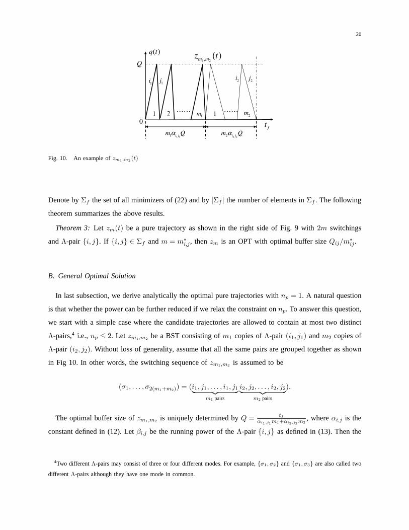
Fig. 10. An example ofzm1,m2(t)
Denote byΣf the set of all minimizers of (22) and by|Σf | the number of elements inΣf . The following
theorem summarizes the above results.
Theorem 3: Let zm(t) be a pure trajectory as shown in the right side of Fig. 9 with2m switchings
andΛ-pair i, j. If i, j ∈ Σf andm = m∗i,j, thenzm is an OPT with optimal buffer sizeQij/m
∗ij .
B. General Optimal Solution
In last subsection, we derive analytically the optimal puretrajectories withnp = 1. A natural question
is that whether the power can be further reduced if we relax the constraint onnp. To answer this question,
we start with a simple case where the candidate trajectoriesare allowed to contain at most two distinct
Λ-pairs,4 i.e., np ≤ 2. Let zm1,m2be a BST consisting ofm1 copies ofΛ-pair (i1, j1) andm2 copies of
Λ-pair (i2, j2). Without loss of generality, assume that all the same pairs are grouped together as shown
in Fig 10. In other words, the switching sequence ofzm1,m2is assumed to be
(σ1, . . . , σ2(m1+m2)) = (i1, j1, . . . , i1, j1︸ ︷︷ ︸
m1 pairs
i2, j2, . . . , i2, j2︸ ︷︷ ︸
m2 pairs
).
The optimal buffer size ofzm1,m2is uniquely determined byQ = tf
αi1,j1m1+αi2,j2
m2, whereαi,j is the
constant defined in (12). Letβi,j be the running power of theΛ-pair i, j as defined in (13). Then the
4Two differentΛ-pairs may consist of three or four different modes. For example, σ1, σ2 andσ1, σ3 are also called two
different Λ-pairs although they have one mode in common.

21
total energy consumed byzm1,m2is computed as
E(m1,m2) = 2(m1 + m2)ks+
pbt2f + βi1,j1αi1,j1m1tf + βi2,j2αi2,j2m2tf
αi1,j1m1 + αi2,j2m2.
Lemma 4: For any i1, j1 and i2, j2, there exists a pair of nonnegative integers(m∗1,m
∗2) with
eitherm∗1 = 0 or m∗
2 = 0 such thatE(m∗1,m
∗2) ≤ E(m1,m2), for any other pair of nonnegative integers
(m1,m2),
Proof: For simplicity, definea1 = βi1,j1αi1,j1tf , a2 = βi2,j2αi2,j2tf andc = pbt2f . Relaxm1, m2 to
nonnegative real numbersx1 andx2. Then
E(x1, x2) = 2ks(x1 + x2) +a1x1 + a2x2 + c
αi1,j1x1 + αi2,j2x2.
Note that all the constantsa1, a2, c, αi1,j1 , andαi2,j2 are positive. To prove the lemma, it suffices to
show that there exists a point on thex1 or x2 axis that minimizesE(x1, x2) in the first quadrant. To
find the minimizers ofE(x1, x2) in the first quadrant, we can first minimize it along each ray inthe
first quadrant, and then find the ray that gives the best minimum value. Towards this purpose, consider
x2 = λx1, whereλ ∈ [0,∞]. Then
E(x1, λx1) =2ks(1 + λ)x1 +(a1 + a2λ)x1 + c
(αi1,j1 + αi2,j2λ)x1
≥2
√
2ks(1 + λ)c
αi1,j1 + αi2,j2λ+
(a1 + a2λ)
(αi1,j1 + αi2,j2λ)
,E(x∗1, λx∗
1).
ThusE(x∗1, λx∗
1) is the minimum value achieved on the rayx2 = λx1. To prove the lemma, it suffices to
show that eitherλ = 0 or λ = ∞ minimizesE(x∗1, λx∗
1). After some computations,E(x∗1, λx∗
1) reduces
to
E(x∗1, λx∗
1) = d3
√
d2y +1
αi2,j2
+ d1y +a2
αi2,j2
, f(y),
wherey = 1α2
i2,j2λ+αi1,j1
αi2,j2
andd1 = a1αi2,j2 − a2αi1,j1 , d2 = αi2,j2 − αi1,j1 andd3 = 2√
2ksc are all
constants. Note that exceptd1 andd2, all the other constants are positive. Asλ increases from0 to ∞,
y decreases from 1αi1,j1
αi2,j2
to 0. Hence, it suffices to show that either0 or 1αi1,j1
αi2,j2
is a minimizer of
f(y) in [0, 1αi1,j1
αi2,j2
]. Note that the second-order derivative off(y) is
d2f
dy2(y) = − d2
2d3
4(d2y + 1/αi2,j2)3/2
≤ 0.
22
Thusf(y) is a concave function ofy in [0, 1αi1,j1
αi2,j2
]. Since the minimizer of a concave function over a
bounded set must be on the boundary of the set, we conclude that either0 or 1αi1,j1
αi2,j2
is a minimizer
of f(y) in [0, 1αi1,j1
αi2,j2
].
According to Lemma 4, for any given twoΛ-pairs, we can always use one of them to construct a pure
trajectory that performs equally well or better than all theother mixed trajectories involving these two
Λ-pairs. Therefore, the following corollary follows immediately.
Corollary 1: The OPT is an optimal solution to Problem 1 under an additional constraintnp ≤ 2.
The question now becomes that whether more energy can be saved by further relaxing the constraint
on np. It turns out to be not the case. In fact, the OPT is an optimal solution to Problem 1 for an arbitrary
np. This can be proved by induction. The following lemma is the key of the induction procedure.
Lemma 5: For any BSTz with length tf andnp = l + 1, there exists another BSTz with length tf
andnp ≤ l that consumes equal or less power thanz.
The proof of Lemma 5 can be found in Appendix . By this lemma, any BST corresponds to a pure
trajectory with no more power consumption. Thus the following theorem follows immediately.
Theorem 4: The OPT defined in Theorem 3 is an OS2 for an arbitrarynp.
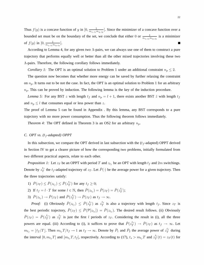
C. OPT vs. (tf -adapted) OPPT
In this subsection, we compare the OPT derived in last subsection with the (tf -adapted) OPPT derived
in Section IV to get a clearer picture of how the corresponding two problems, initially formulated from
two different practical aspects, relate to each other.
Proposition 1: Let zT be an OPPT with periodT andztfbe an OPT with lengthtf and2m switchings.
Denote byztf
T the tf -adapted trajectory ofzT . Let P (·) be the average power for a given trajectory. Then
the three trajectories satisfy:
1) P (zT ) ≤ P (ztf) ≤ P (z
tf
T ) for any tf ≥ 0;
2) If tf = l · T for somel ∈ N, then P (ztf) = P (zT ) = P (z
tf
T );
3) P (ztf) → P (zT ) and P (z
tf
T ) → P (zT ) as tf → ∞.
Proof: (i) Obviously P (ztf) ≤ P (z
tf
T ) as ztf
T is also a trajectory with lengthtf . Since zT is
the best periodic trajectory,P (zT ) ≤ P (P[ztf]) = P (ztf
). The desired result follows. (ii) Obviously
P (zT ) = P (ztf
T ) as ztf
T is just the firstl periods ofzT . Considering the result in (i), all the three
powers are equal. (iii) According to (i), it suffices to provethat P (ztf
T ) → P (zT ) as tf → ∞. Let
mtf= ⌊tf/T ⌋. Thenmtf
T/tf → 1 as tf → ∞. Denote byP1 and P2 the average power ofztf
T during
the interval[0,mtfT ] and [mtf
T, tf ], respectively. According to (17),ts > mtfT andz
tf
T (t) = zT (t) for

23
TABLE I
POWER MODES OF SYSTEMH1
modei 1 2 3 4 5 6
ri 0 1 2 3 4 5
pi 0.1 0.12 0.2 0.3 0.33 0.4
t ∈ [0,mtfT ]. Thus P1 = P (zT ). Note thatP2 ≤ pN + 2ks
tf−mtfT + pbQ, wherepN is the power of the
highest mode. Hence, astf → ∞,
P (ztf
T ) =P1mtf
T + P2(tf − mtfT )
tf→ P (zT ).
Remark 3: Any practical application corresponds to a finitetf . If the tf is unknown, we can only
compute the OPPT (zT ). Applying zT to the application results in atf -adapted trajectoryztf
T . On the
other hand, iftf is known a priori, a better trajectory (ztf) than z
tf
T can be computed. In fact,ztfis
the best trajectory for the giventf and its power is bounded from below byP (zT ) and from above by
P (ztf
T ).
VI. SIMULATION
A. Fictional Example
Consider a system (H1) with 6 power modes as defined in Table I.Assume thatks = 0.1, pb = 0.1
andry = 3.5. For this system H1, we compute the OPPT (zT ), the OPT (ztf) and thetf -adapted OPPT
(ztf
T ), according to Theorem 1, Theorem 4 and equation (17), respectively. Denote byP (·) the average
power of a given trajectory. In Fig. 11-(a), we plot the powerof each trajectory as a function oftf . It
can be seen thatP (ztf) always stays belowP (z
tf
T ) and both of them converge toP (zT ) from above as
tf → ∞. It is also observed that the three trajectories have the same average power whentf is an integer
multiple of the optimal period (T = 2.8284) of the OPPT. These observations are consistent with our
analysis in Section V-C. In Fig. 11-(b), we plot the optimalΛ-pairs ofzT andztfas functions oftf . It
can be seen that the optimalΛ-pair in ztfis initially 5, 2 and eventually converges to5, 4 which is
the optimalΛ-pair of zT (andztf
T ). This indicates thatztfmay involve differentΛ-pairs for differenttf .
24
0 2 4 6 8 10 12 14 16 18 200.45
0.5
0.55
0.6
0.65
0.7
0.75
0.8
t f
Pow
er
OPPTOPTtf−adapted OPPT
tf=T
(a) Convergence of powers
0 0.5 1 1.5 2 2.5 3
t f
Λ p
air
OPTOPPT
Λ−pair (5,2)
Λ−pair (5,3)
Λ−pair (5,4)
(b) Λ-pairs in the OPPT and OPT
Fig. 11. Simulation results of example 1
B. Practical Example
Our theoretical results can be applied in many real-world applications, such as the power management
problem of a multiple-speed disk ([5]) and the dynamic voltage scheduling (DVS) problem of a variable
speed processor ([4]). In this section, we use a DVS example to illustrate the effectiveness of our results.
Let X be an Intel Xscal processor ([23]) with five available power modes as defined in Table II. Suppose
that Y is a video card that fetches data from X at a constant speed 8 Mbps (1MB/s). The power per
megabyte for buffer B can be looked up in the datasheet ([24])as6.258× 10−4 W/MB. A typical value
of the switching energy is 0.1mJ in a microprocessor ([4]). Since the switching costks in our model may

25
TABLE II
POWER MODES OFINTEL XSCALE PROCESSOR
modei 1 2 3 4 5
fi (MHz) 150 400 600 800 1000
ri (MB/s) 0.45 1.2 1.8 2.4 3
pi (Watt) 0.08 0.17 0.4 0.9 1.6
also include other switching penalties, such as the switching delay penalty, we test our method forks
ranging from 0.1mJ to 100mJ. Astf is usually large for video programs, thetf -adapted OPPT and the
OPT will provide almost the same power performance. For simplicity we only implement thetf -adapted
OPPT in this simulation and refer to this method as Scheme 1. Aheuristic strategy, referred to as Scheme
2, is also implemented where X is switched to the highest speed until the buffer is full and then switched
to the lowest speed until the buffer is empty. Scheme 2 is tested for four heuristically selected buffer
sizes 0.1MB, 0.3MB, 1MB and 8MB. The power consumptions of Scheme 2 in these cases are compared
with Scheme 1 in Fig. 12. It can be seen that the proposed optimal strategy always performs the best for
eachks and can save about 60% of power consumption compared with theheuristic ones.
VII. C ONCLUSIONS
This paper introduces a modeling framework for the DBM problem using hybrid systems. Two
practically important DBM problems are formulated as optimal control problems of a piecewise constant
hybrid system. Various necessary conditions are derived using some variational approach. It is shown that
the optimal pure trajectory (OPT) and the optimal pure periodic trajectory (OPPT) are optimal solutions
to Problems 1 and 2, respectively. General guidelines for solving practical DMB problems using these
optimal strategies are also discussed. For a particular application, if its time horizontf is unknown,
one can only compute the OPPT. Applying the OPPT to the application results in atf -adapted OPPT,
which is a good suboptimal strategy that converges to the true optimal strategy astf goes to infinity. On
the other hand, iftf is known, the best strategy OPT can computed, which guarantees the least energy
consumption for this particular application. Future research will focus on the following two aspects: one
is to extend our analysis to the case where more than one buffers are inserted among multiple streamlined
components. The other one is to study the case where the data rates of components are varying or even
random instead of constant.

26
0 0.01 0.02 0.03 0.04 0.05 0.06 0.07 0.08 0.09 0.10
0.2
0.4
0.6
0.8
1
k s
(J)
Nor
mal
ized
Pow
er
Scheme1Scheme2(Q=0.1MB)Scheme2(Q=0.3MB)Scheme2(Q=1MB)Scheme2(Q=8MB)
Fig. 12. Power consumptions of various methods under different ks. For eachks, all the powers are normalized w.r.t. the
largest one.
APPENDIX
Proof: Let z(t) = (q(t), σ(t)) be an OS1 with switching instants(t0, . . . , tn−1) and buffer sizeQ.
Supposeq(ti) ∈ (0, Q) for somei. Definezh as in (6) withT replaced bytf . Thenzh has the same
buffer sizeQ as z, and similar to (9), its length isthf = ti−1 + t(2)h + (tf − ti+1), wheret
(2)h is given
in (7). Definezh = Sch[zh], wherech = tf/thf . According to the properties of the scaling operation, the
buffer size ofzh becomescQ and the length ofzh is changed back totf . Therefore,zh is a feasible
trajectory for Problem 1. Considering (3) and (10), the power of zh is computed as
P (zh;Q, tf ) =1
thf
[E1 + E3 + 2ks + pσi
· h
+ pσi+1(t
(2)h − h)
]+ pbchQ +
nks(1 − ch)
chthf.

27
Taking the derivative ofP (zh;Q, tf ) with respect toh, we have
dP (zh;Q, tf )
dh=
1(
thf
)2
[(
pσi+ pσi+1
ry − rσi
rσi+1− ry
)
·(
tf − (ti+1 − ti−1) +q2 − q1
rσi+1− ry
)
−(
1 +ry − rσi
rσi+1− ry
)
·(
E1 + E3 + ks + pσi+1
q2 − q1
rσi+1− ry
)]
+nks − pbQtf
(thf )2
(
1 − ry − rσi
rσi+1− ry
)
.
Therefore,P (zh;Q, tf ) is monotone with respect toh as the sign ofdP (zh;Q,tf )dh does not depend onh.
Using the same argument as in the last paragraph of the proof of Lemma 2, it follows that the optimal
solution to Problem 1 must also be a BST.
Q
( )q t
0
……
ft
1 1m 1 1lm
1i 1j 1li1lj
……1
2m……
a
2i 2j
……
1z 2z
Fig. 13. A trajectoryz with np = l + 1
Proof: Without loss of generality, assume thatz is as shown in Fig. 13 with the following switching
sequence
(i1, j1, . . . , i1, j1︸ ︷︷ ︸
m1 pairs
, . . . , il+1, jl+1, . . . , il+1, jl+1︸ ︷︷ ︸
ml+1 pairs
).
Definez1 = C0,a[z] andz2 = Ca,tf[z], wherea is the starting time of the first copy ofi2, j2 as shown
in Fig. 13. Letσ+, σ− be a (virtual)Λ-pair whose data rates and powers are defined as
rσ+= ry +
2Q
tf, rσ−
= ry −2Q
tf,
pσ+=
l+1∑
k=2
pik(τik
)
tf − a, pσ−
=
l+1∑
k=2
pjk(τjk
)
tf − a,
(23)

28
Q
( )q t
0ft
1 1lm
1li1lj
……1
2m……
2i 2j
……
2z
Q
( )q t
0
2z
ft
Q
( )q t
0ft
2[ ]c z
… … … … … ………
2[ ]c z
2[ ]m c z
Q
( )q t
0ft
2ˆ[ ]c z
……
2ˆ[ ]c z
2ˆ[ ]m cz z
(a) (b)
Fig. 14. (a) Two-mode representation ofz2; (b) The Optimal trajectoryz and its corresponding original trajectory
whereτikis the total timez2 spends in modeik. Thuspσ+
andpσ−in the above equation represent the
average powers of all the ascending modes and the descendingmodes ofz2, respectively. Note that the
so defined modesσ+ and σ− may not be feasible modes inS. They are only introduced to simplify
the proof. Letz2 be aΛ-trajectory with the virtual modesσ+, σ− as shown in Fig. 14-(a). Define the
switching cost inz2 to be2lks/2. Thenz2 has the same buffer size and total energy asz2; thusJ [z1, z2]
consumes the same energy asz. On the other hand,J [z1, z2] is a mixed trajectory withnp = 2; its
two different Λ-pairs σ+, σ− and i1, j1 appear 1 andm1 times, respectively. By Lemma 4, there
exists a pure trajectoryz involving only the pairi1, j1 or σ+, σ− that consumes no more energy
thanJ [z1, z2].5 Thus z also consumes no more energy thanz. If z involves only the pairi1, j1, then
it is a pure trajectory (np = 1) satisfying all the constraints in Problem 1 with no more energy than
z. On the other hand, ifz involves only the pairσ+, σ−, it may not satisfy the third constraint in
Problem 1 asσ+ andσ− may not be inS. In this case,z must consist of a series of a scaled version of
z2, i.e., z = Jm[Sc[z2]] for somem andc. According to (23),Jm[Sc[z2]] (obtained by replacing everyz2
5Note thatσ+, σ− andi1, j1 have different switching costs. However, with slight modifications, Lemma 4 also applies
for the case where the twoΛ-pairs have different switching costs.

29
with z2) as shown in Fig 14-(b) consumes the same energy asz. Thus we obtain a trajectoryJm[Sc[z2]]
with np = l (involving only the valid modesi2, j2, . . . , il+1, jl+1) that consumes no more energy thanz.
Hence, in either case we can find a trajectory withnp ≤ l that satisfies all the constraints in Problem 1
and consumes no more power thanz.
REFERENCES
[1] L. Cai and Y.-H. Lu, “Energy management using buffer memory for streaming data,”IEEE Transactions on Computer-Aided
Design of Integrated Circuits and Systems, vol. 24, no. 2, pp. 141–152, 2005.
[2] J. Hu and Y.-H. Lu, “Buffer management for power reduction using hybrid control,” inProceedings of the IEEE Conference
on Decision and Control, (Seville, Spain), pp. 6997–7002, 2005.
[3] J. Ridenour, J. Hu, N. Pettis, and Y.-H. Lu, “Low-power buffer management for streaming data,”IEEE Transactions on
Circuits and Systems for Video Technology, vol. 17, no. 2, pp. 143–157, 2007.
[4] T. D. Burd and R. W. Brodersen, “Design issues for dynamicvoltage scaling,” inProceedings of the international symposium
on Low power electronics and design, pp. 9–14, ACM Press, 2000.
[5] S. Gurumurthi, A. Sivasubramaniam, M. Kandemir, and H. Franke, “Drpm: Dynamic speed control for power management
in server class disks.,” inProceedings of the International Symposium on Computer Architecture (ISCA), pp. 169–179,
June 2003.
[6] R. Alur, T. Henzinger, G. Lafferriere, and G. J. Pappas, “Discrete abstractions of hybrid systems,”Proceedings of the
IEEE, vol. 88, no. 2, pp. 971–984, 2000.
[7] M. S. Branicky, V. S. Borkar, and S. K. Mitter, “A unified framework for hybrid control: model and optimal-control theory,”
IEEE Transactions on Automatic Control, vol. 43, no. 1, pp. 31–45, 1998.
[8] S. Hedlund and A. Rantzer, “Optimal control of hybrid system,” in Proceedings of the IEEE Conference on Decision and
Control, vol. 4, (Phoenix, AZ), pp. 3972–3977, December 1999.
[9] X. Xu and P. Antsaklis, “A dynamic programming approach for optimal control of switched systems,” inProceedings of
the IEEE Conference on Decision and Control, (Sydney, Australia), pp. 1822–1827, December 2000.
[10] X. Xu and P. Antsaklis, “Optimal control of switched systems: new results and open problems,” inProceedings of the
American Control Conference, (Chicago, IL), pp. 2683–2687, June 2000.
[11] P. Riedinger, F. Kratz, C. Iung, and C. Zanne, “Linear quadratic optimization for hybrid systems,” inProceedings of the
IEEE Conference on Decision and Control, (Phoenix, AZ), pp. 3059–3064, December 1999.
[12] P. Riedinger, C. Zanne, and F. Kratz, “Time optimal control of hybrid systems,” inProceedings of the American Control
Conference, (San Diego, CA), pp. 2466–2470, June 1999.
[13] H. J. Sussmann, “A maximum principle for hybrid optimalcontrol problems,” inProceedings of the IEEE Conference on
Decision and Control, (Phoenix, AZ), pp. 425–430, December 1999.
[14] B. Piccoli, “Hybrid systems and optimal control,” inProceedings of the IEEE Conference on Decision and Control, (Tampa,
FL), pp. 13–18, December 1998.
[15] X. Xu and P. Antsaklis, “Optimal control of switched systems based on parameterization of the switching instants,”IEEE
Transactions on Automatic Control, vol. 49, no. 1, pp. 2–16, 2004.
[16] M. Egerstedt, Y. Wardi, and F. Delmotte, “Optimal control of switching times in switched dynamical systems,”IEEE
Transactions on Automatic Control, vol. 51, no. 1, pp. 110–115, 2006.

30
[17] S. C. Bengea and R. A. DeCarlo, “Optimal control of switching systems,”Automatica, vol. 41, no. 1, pp. 11–27, 2005.
[18] C. G. Cassandras, D. L. Pepyne, and Y. Wardi, “Optimal control of a class of hybrid systems,”IEEE Transactions on
Automatic Control, vol. 46, no. 3, pp. 398–415, 2001.
[19] L. Y. Wanga, A. Beydoun, J. Cook, J. Sun, and I. Kolmanovsky, “Optimal hybrid control with applications to automotive
powertrain systems,” inControl Using Logic-Based Switching, vol. 222, (London, UK), pp. 190–200, Springer-Verlag,
1997.
[20] K. Gokbayrak and C. Cassandras, “A hierarchical decomposition method for optimal control of hybrid systems,” in
Proceedings of the IEEE Conference on Decision and Control, vol. 2, (Sydney, NSW, Australia), pp. 1816–1821, December
2000.
[21] K. Gokbayrak and C. G. Cassandras, “Hybrid controllersfor hierarchically decomposed systems,” inHSCC ’00: Proceedings
of the Third International Workshop on Hybrid Systems: Computation and Control, (London, UK), pp. 117–129, Springer-
Verlag, 2000.
[22] Y.-H. Lu, L. Benini, and G. D. Micheli, “Dynamic frequency scaling with buffer insertion for mixed workloads,”IEEE
Transactions on Computer-Aided Design of Integrated Circuits and Systems, vol. 21, no. 11, pp. 1284–1305, 2002.
[23] R. Xu, C. Xi, R. Melhem, and D. Moss, “Practical pace for embedded systems,” inEMSOFT ’04: Proceedings of the 4th
ACM international conference on Embedded software, pp. 54–63, ACM Press, 2004.
[24] Rambus-Inc., “Rambus 128/144-mbit direct rdram data sheet,” June 2000.