research article comparative sensitivity analysis...

Research ArticleComparative Sensitivity Analysis of Muscle Activation Dynamics

Robert Rockenfeller,1 Michael Günther,2,3 Syn Schmitt,2,4 and Thomas Götz1

1 Institut fur Mathematik, Universitat Koblenz, 56070 Koblenz, Germany2Institut fur Sport- und Bewegungswissenschaft, Universitat Stuttgart, Allmandring 28, 70569 Stuttgart, Germany3Institut fur Sportwissenschaft, Lehrstuhl fur Bewegungswissenschaft, Friedrich-Schiller-Universitat,Seidelstraße 20, 07749 Jena, Germany4Stuttgart Research Centre for Simulation Technology, Pfaffenwaldring 7a, 70569 Stuttgart, Germany

Correspondence should be addressed to Michael Gunther; [email protected]

Received 15 December 2014; Accepted 5 February 2015

Academic Editor: Eduardo Soudah

Copyright © 2015 Robert Rockenfeller et al. This is an open access article distributed under the Creative Commons AttributionLicense, which permits unrestricted use, distribution, and reproduction in any medium, provided the original work is properlycited.

We mathematically compared two models of mammalian striated muscle activation dynamics proposed by Hatze and Zajac. Bothmodels are representative for a broad variety of biomechanical models formulated as ordinary differential equations (ODEs).Thesemodels incorporate parameters that directly represent known physiological properties. Other parameters have been introducedto reproduce empirical observations. We used sensitivity analysis to investigate the influence of model parameters on the ODEsolutions. In addition, we expanded an existing approach to treating initial conditions as parameters and to calculating second-order sensitivities. Furthermore, we used a global sensitivity analysis approach to include finite ranges of parameter values. Hence,a theoretician striving for model reduction could use the method for identifying particularly low sensitivities to detect superfluousparameters. An experimenter could use it for identifying particularly high sensitivities to improve parameter estimation. Hatze’snonlinear model incorporates some parameters to which activation dynamics is clearly more sensitive than to any parameter inZajac’s linear model. Other than Zajac’s model, Hatze’s model can, however, reproduce measured shifts in optimal muscle lengthwith variedmuscle activity. Accordingly we extracted a specific parameter set for Hatze’s model that combines best with a particularmuscle force-length relation.

1. Introduction

Scientific knowledge is gained by an interplay betweenquantitative real world measurements of physical, chemical,or biological phenomena and the development of mathe-matical models for understanding the dynamical processesbehind. In general, such phenomena are determined as spa-tiotemporal patterns of physical measures (state variables).Modelling consists of distinguishing the surrounding worldfrom the system that yields the phenomena and formulatinga mathematical description of the system, a model, that canpredict values of the state variables. The calculations dependon model parameters and often on giving measured inputvariables. By changing parameter values and analysing theresulting changes in the values of the state variables, themodel may then be used as a predictive tool. This way, the

model’s validity can be verified. If the mathematical modeldescription is moreover derived from first principles, themodel has the potential to explain the phenomena in a causalsense.

Calculating the sensitivities of amodel’s predicted output,that is, the system’s state variables, with respect to modelparameters is a means of eliminating redundancy and inde-terminacy frommodels and thus helps to identify valid mod-els. Sensitivity analyses can be helpful both in model-basedexperimental approaches and in purely theoretical work. Amodelling theoretician could be looking for parameters towhich all state variables are nonsensitive. Such parametersmight be superfluous. An experimenter may inspect themodel that represents his working hypothesis and analysewhich of the model’s state variables are specifically sensitiveto a selected parameter. Hence, the experimenter would have

Hindawi Publishing CorporationComputational and Mathematical Methods in MedicineVolume 2015, Article ID 585409, 16 pageshttp://dx.doi.org/10.1155/2015/585409

2 Computational and Mathematical Methods in Medicine

to measure exactly this state variable to identify the value ofthe selected parameter.

In a biomechanical study Scovil and Ronsky [1] appliedsensitivity analysis to examine the dynamics of a mechanicalmultibody system: a runner’s skeleton coupled to muscleactivation-contraction dynamics. They calculated specificsensitivity coefficients in three slightly different ways. Asensitivity coefficient is the difference quotient calculatedfrom dividing the change in a state variable by the changein a model parameter value, evaluated in a selected systemstate [2]. The corresponding partial derivative may be simplycalled “sensitivity.” Therefore, a sensitivity function is thetime evolution of a sensitivity [2]. Accordingly, Lehman andStark [2] had proposed a more general and unified approachthan Scovil and Ronsky [1], which allows systematically cal-culating the sensitivities of any dynamical system describedin terms of ordinary differential equations. As an examplefor sensitivity functions, Lehman and Stark [2] had appliedtheir proposed method to a muscle-driven model of saccadiceye movement. By calculating a percentage change in a statevariable value per percentage change in a parameter value, allsensitivities can be made comprehensively comparable, evenacross models.

A sensitivity as defined so far is of first order. Method-ically, we aim at introducing a step beyond, namely, atcalculating second order sensitivities. These measures aresuited to quantify howmuch the sensitivity of a state variablewith respect to one model parameter depends on changinganother parameter. By analysing second order sensitivities,the strength of their interdependent influence on modeldynamics can be determined. In addition to this so-calledlocal sensitivity analysis, we will take the whole parametervariability into account by calculating global sensitivitiesaccording to Chan et al. [3] and Saltelli and Chan [4]. Thisapproach allows translating the impact of one parameter ona state variable into a parameter’s importance, by completelycomprising its interdependent influence in combination withall other parameters’ sensitivities.

In this study, we will apply the sensitivity analysis tomodels that predict how the activity of a muscle (its chemicalstate) changeswhen themuscle is stimulated by neural signals(electrical excitation). Such models are used for simulationsofmuscles’ contractions coupled to their activation dynamics.Models for coupled muscular dynamics are often part ofneuromusculoskeletal models of biological movement sys-tems. In particular, we want to try and rate two specificmodel variants of activation dynamics formulated by Zajac[5] and by Hatze [6]. As a first result, we present an exampleof a simplified version of the Zajac [5] model, in whichsensitivity functions can in fact be calculated in closed form.Subsequently we calculate the sensitivities numerically withrespect to all model parameters in both models, aiming atan increased understanding of the influence of changes inmodel parameters on the solutions of the underlying ordinarydifferential equations (ODEs). Additionally, we discuss whichof both models may be physiologically more accurate. Thearguments come from a mixture of three different aspects:sensitivity analysis, others’ experimental findings, and an

additional attempt to best fit different combinations of acti-vation dynamics and force-length relations of the contractileelement (CE) in a muscle to known data on shifts in optimalCE length with muscle activity [7].

2. Two Models forMuscle Activation Dynamics

Macroscopically, a muscle fibre or an assembly thereof, amuscle belly, is often mapped mathematically by a one-dimensional massless thread called “contractile component”or “contractile element” (CE) [8–12]. Its absolute length isℓCE which may be normalised to the optimal fibre lengthℓCE,opt by ℓCErel = ℓCE/ℓCE,opt. In macroscopic muscle models,the CE muscle force is usually modelled as a function ofa force-(CE-)length relation, a force-(CE-)velocity relation,and (CE-)activity 𝑞. Commonly the muscle activity 𝑞 rep-resents the number of attached cross-bridges within themuscle, normalised to the maximum number available (𝑞

0

≤

𝑞 ≤ 1). It can also be considered as the concentration ofbound Ca2+-ions in the muscle sarcoplasma relative to itsphysiological maximum. The parameter 𝑞

0

represents theminimum activity that is assumed to occur without anystimulation [6].

We analyse two different formulations of muscle activa-tion dynamics, that is, the time (its symbol: 𝑡) evolution ofmuscle activity 𝑞(𝑡). One formulation of muscle activationdynamics was suggested by Zajac [5], which we modifiedslightly to take 𝑞

0

into account:

𝑞𝑍

=1

𝜏 ⋅ (1 − 𝑞0

)⋅ [𝜎 ⋅ (1 − 𝑞

0

) − 𝜎 ⋅ (1 − 𝛽) ⋅ (𝑞𝑍

− 𝑞0

)

−𝛽 ⋅ (𝑞𝑍

− 𝑞0

)] ,

(1)

with the initial condition 𝑞𝑍

(0) = 𝑞𝑍,0

. In this context, 𝜎is supposed to represent the (electrical) stimulation of themuscle, being a parameter for controlling muscle dynamics.It represents the output of the nervous system’s dynamicsapplied to the muscle which in turn interacts with the skele-ton, the body mass distribution, the external environment,and therefore the nervous system in a feedback loop. Elec-tromyographic (EMG) signals can be seen as a compound ofsuch neural stimulations collected in a finite volume (beingthe input to a number of muscle fibres) over a frequencyrange and coming from a number of (moto-)neurons. Theparameter 𝜏 denotes the activation time constant, and 𝛽 =𝜏/𝜏deact is the ratio of activation to deactivation time constants(deactivation boost).

An alternative formulation ofmuscle activation dynamicswas introduced by Hatze [6]:

𝛾 = 𝑚 ⋅ (𝜎 − 𝛾) . (2)

We divided the original equation from Hatze [6] by theparameter 𝑐 = 1.37 ⋅ 10

−4mol/L which represents themaximum concentration of free Ca2+-ions in the muscle sar-coplasma. Thus, the values of the corresponding normalised

Computational and Mathematical Methods in Medicine 3

concentration are 0 ≤ 𝛾 ≤ 1. The activity is finally calculatedby the function

𝑞𝐻

(𝛾, ℓCErel) =𝑞0

+ [𝜌 (ℓCErel) ⋅ 𝛾]]

1 + [𝜌 (ℓCErel) ⋅ 𝛾]] , (3)

and the parameter 𝑐 is shifted to the accordingly renormalisedfunction

𝜌 (ℓCErel) = 𝜌𝑐 ⋅ℓ𝜌

− 1

ℓ𝜌

/ℓCErel − 1, (4)

with 𝜌𝑐

= 𝑐⋅𝜌0

and ℓ𝜌

= 2.9. Two cases have been suggested byHatze [13]: 𝜌

0

= 6.62 ⋅ 104 L/mol (i.e., 𝜌

𝑐

= 9.10) for ] = 2 and𝜌0

= 5.27 ⋅ 104 L/mol (i.e., 𝜌

𝑐

= 7.24) for ] = 3, which havebeen applied in the literature [7, 8, 14, 15]. By substituting (2)and (3) into 𝑞

𝐻

= 𝑑𝑞𝐻

(𝛾, ℓCErel)/𝑑𝛾 ⋅ 𝛾 and resubstituting theinverse of (3) afterwards, Hatze’s formulation of an activationdynamics can be transformed into a nonlinear differentialequation directly in terms of the activity:

𝑞𝐻

=] ⋅ 𝑚1 − 𝑞0

⋅ [𝜎 ⋅ 𝜌 (ℓCErel) ⋅ (1 − 𝑞𝐻)1+1/]⋅ (𝑞𝐻

− 𝑞0

)1−1/]

− (1 − 𝑞𝐻

) ⋅ (𝑞𝐻

− 𝑞0

)] ,

(5)

with the initial condition 𝑞𝐻

(0) = 𝑞𝐻,0

.The solutions 𝑞

𝑍

(𝑡) and 𝑞𝐻

(𝑡) of both formulations ofactivation dynamics (1) and (5) can now be directly comparedby integrating them with the same initial condition 𝑞

𝑍,0

=

𝑞𝐻,0

using the same stimulation 𝜎.

3. Local First and Second Order Sensitivity ofODE Systems regarding Their Parameters

Let Ω ⊆ R × R𝑀 × R𝑁 and 𝑓 : Ω → R𝑀. We then considera system of ordinary, first order initial value problems (IVP):

�� = 𝑓 (𝑡, 𝑌 (𝑡, Λ) , Λ) , 𝑌 (0) = 𝑌0

, (6)

where 𝑌(𝑡) = (𝑦1

(𝑡), 𝑦2

(𝑡), . . . , 𝑦𝑀

(𝑡)) denotes the vectorof state variables, 𝑓 = (𝑓

1

, 𝑓2

, . . . , 𝑓𝑀

) the vector of righthand sides of the ODE, and Λ = {𝜆

1

, 𝜆2

, . . . , 𝜆𝑁

} the set ofparameters which the ODE depends on. The vector of initialconditions is abbreviated by

𝑌 (0) = (𝑦1

(0) , 𝑦2

(0) , . . . , 𝑦𝑀

(0))

= (𝑦1,0

, 𝑦2,0

, . . . , 𝑦𝑀,0

) = 𝑌0

.

(7)

The first order sensitivity of the solution 𝑌(𝑡, Λ) withrespect to the parameter set Λ is defined as the matrix

𝑆 (𝑡, Λ) = (𝑆𝑖𝑘

(𝑡, Λ))𝑖=1,...,𝑁,𝑘=1,...,𝑀

,

with 𝑆𝑖𝑘

(𝑡, Λ) =𝑑

𝑑𝜆𝑖

𝑦𝑘

(𝑡, Λ) .

(8)

Simplifying, we denote 𝑌 = 𝑌(𝑡, Λ), 𝑓 = 𝑓(𝑡, 𝑌, Λ), and𝑆𝑖𝑘

= 𝑆𝑖𝑘

(𝑡, Λ) but keep the dependencies in mind. Because

the solution 𝑌(𝑡) might only be gained numerically ratherthan in a closed-form expression, we have to apply the well-known theory of sensitivity analysis as stated in Vukobratovic[16], Dickinson and Gelinas [17], Lehman and Stark [2], andZivariPiran [18]. Differentiating (8) with respect to 𝑡 andapplying the chain rule yield

𝑑

𝑑𝑡𝑆𝑖𝑘

=𝑑2

𝑑𝑡𝑑𝜆𝑖

𝑦𝑘

=𝑑2

𝑑𝜆𝑖

𝑑𝑡𝑦𝑘

=𝑑

𝑑𝜆𝑖

𝑓𝑘

=𝑑

𝑑𝜆𝑖

𝑌 ⋅𝜕

𝜕𝑌𝑓𝑘

+𝜕

𝜕𝜆𝑖

𝑓𝑘

,

(9)

with 𝜕/𝜕𝑌 being the gradient of state variables. Hencewe obtain the following ODE for the first order solutionsensitivity:

𝑆𝑖𝑘

=

𝑀

∑

𝑙=1

𝑆𝑖𝑙

⋅𝜕

𝜕𝑦𝑙

𝑓𝑘

+𝜕

𝜕𝜆𝑖

𝑓𝑘

, 𝑆𝑖𝑘

(0) =𝜕

𝜕𝜆𝑖

𝑦𝑘,0

= 0,

(10)

or in short terms

𝑆 = 𝑆 ⋅ 𝐽 + 𝐵, 𝑆 (0) = 0𝑁×𝑀

, (11)

where 𝑆 = 𝑆(𝑡) is the𝑁×𝑀 sensitivity matrix and 𝐽 = 𝐽(𝑡) isthe𝑀×𝑀 Jacobianmatrix with 𝐽

𝑘𝑙

= (𝜕/𝜕𝑦𝑙

)𝑓𝑘

; furthermore,𝐵 = 𝐵(𝑡) denotes the 𝑁 × 𝑀-matrix containing the partialderivatives 𝐵

𝑖𝑘

= (𝜕/𝜕𝜆𝑖

)𝑓𝑘

and 0𝑁×𝑀

denotes the 𝑁 × 𝑀-matrix consisting of zeros only.

By analogy, the second order sensitivity of 𝑌(𝑡) withrespect to Λ is defined as the following𝑁 ×𝑁 ×𝑀-tensor:

𝑅 (𝑡, Λ) = (𝑅𝑖𝑗𝑘

(𝑡, Λ))𝑖,𝑗=1,...,𝑁,𝑘=1,...,𝑀

, (12)

with

𝑅𝑖𝑗𝑘

(𝑡, Λ) =𝑑

𝑑𝜆𝑖

𝑆𝑗𝑘

=𝑑

𝑑𝜆𝑗

𝑆𝑖𝑘

=𝑑2

𝑑𝜆𝑖

𝑑𝜆𝑗

𝑦𝑘

= 𝑅𝑗𝑖𝑘

(𝑡, Λ) ,

(13)

assuming 𝑅𝑖𝑗𝑘

= 𝑅𝑗𝑖𝑘

for all 𝑘 = 1, . . . ,𝑀, therefore assumingthat the prerequisites of Schwarz theorem (symmetry of thesecond derivatives) are fulfilled throughout. Differentiatingwith respect to 𝑡 and applying the chain rule lead to the ODE

��𝑖𝑗𝑘

=

𝑀

∑

𝑙=1

(𝑅𝑖𝑗𝑙

𝜕

𝜕𝑦𝑙

𝑓𝑘

+ 𝑆𝑖𝑙

𝜕

𝜕𝜆𝑗

𝑓𝑘

+ 𝑆𝑗𝑙

𝜕

𝜕𝜆𝑖

𝑓𝑘

)

+

𝑀

∑

𝑙1=1

𝑀

∑

𝑙2=1

𝑆𝑖𝑙1

𝑆𝑗𝑙2

𝜕2

𝜕𝑦𝑙1

𝜕𝑦𝑙2

𝑓𝑘

+𝜕2

𝜕𝜆𝑖

𝜕𝜆𝑗

𝑓𝑘

,

(14)

with 𝑅𝑖𝑗𝑘

(0) = 0. For purposes beyond the aim of this paper,a condensed notation introducing the concept of tensor (orKronecker) products as in ZivariPiran [18] may be helpful.For a practical implementation in MATLAB see Bader andKolda [19].

Furthermore, if an initial condition 𝑦𝑘,0

(see (7)) isconsidered as another parameter, we can derive a separate


sensitivity differential equation by rewriting (6) in its integralform

𝑌 (𝑡) = 𝑌0

+ ∫

𝑡

0

𝑓 (𝑠, 𝑌 (𝑠)) 𝑑𝑠. (15)

Differentiating this equation with respect to 𝑌0

yields

𝑆𝑌0(𝑡) =

𝜕

𝜕𝑌0

𝑌 (𝑡) = 1 + ∫

𝑡

0

𝜕

𝜕𝑌𝑓 ⋅𝜕

𝜕𝑌0

𝑌 (𝑠) 𝑑𝑠 (16)

and differentiating again with respect to 𝑡 results in ahomogeneous ODE for each component 𝑆

𝑦𝑘,0

(𝑡); namely,

𝑆𝑦𝑘,0(𝑡) =

𝑀

∑

𝑙=1

𝜕

𝜕𝑦𝑙

𝑓𝑘

⋅ 𝑆𝑦𝑙,0

, with 𝑆𝑦𝑘,0(0) =

𝜕

𝜕𝑦𝑘,0

𝑦𝑘,0

= 1.

(17)

The parameters of our analysed models are supposed torepresent physiological processes and bear physical dimen-sions therefore. For example,𝑚 and 1/𝜏 are frequencies mea-sured in (Hz), whereas 𝑐 is measured in (mol/L). Accordingly,𝑆𝜏

= (𝑑/𝑑𝜏)𝑞𝑍

would be measured in (Hz) and 𝑆𝑚

in (s)(note that our model only consists of 𝑜𝑛𝑒 ODE and thereforewe do not need a second index). Normalisation providesa comprehensive comparison between all sensitivities, evenacross models. For any parameter, the value 𝜆

𝑖

fixed for aspecific simulation is a natural choice. For any state variable,we chose its current value 𝑦

𝑘

(𝑡) at each point in time ofthe corresponding ODE solution. Hence, we normalise eachsensitivity 𝑆

𝑖𝑘

= 𝑑𝑦𝑘

/𝑑𝜆𝑖

by multiplying it with the ratio𝜆𝑖

/𝑦𝑘

(𝑡) to get the relative sensitivity

𝑆𝑖𝑘

= 𝑆𝑖𝑘

⋅𝜆𝑖

𝑦𝑘

. (18)

A relative sensitivity 𝑆𝑖𝑘

thus quantifies the percentage changein the 𝑘th state variable value per percentage change in the 𝑖thparameter value.This applies accordingly to the second ordersensitivity

��𝑖𝑗𝑘

= 𝑅𝑖𝑗𝑘

⋅

𝜆𝑖

⋅ 𝜆𝑗

𝑦𝑘

. (19)

It can be shown that this method is valid and mathematicallyequivalent to another common method in which the wholemodel is nondimensionalised a priori [20]. A nonnormalisedmodel formulation has the additional advantage of usuallyallowing a more immediate appreciation of and transparentaccess for experimenters. In the remainder of this paper, weare always going to present and discuss relative sensitivityvalues normalised that way.

In our model the specific case𝑀 = 1 applies, so (10) and(14) simplify to the case 𝑘 = 1 (no summation).

4. Variance-Based Global Sensitivity Analysis

The differential sensitivity analysis above is called a localmethod because it does not take the physiological range

of parameter values into account. Additionally factoringin such ranges characterises the so-called global methods.The main idea behind most global methods is to includea statistical component to scan the whole parameter spaceC and combine the percentage change in a state variablevalue per percentage change in a parameter value with thevariability of all of the parameters. The parameter space Ccan be seen as a𝑁-dimensional cuboid C = [𝜆−

1

; 𝜆+

1

] × ⋅ ⋅ ⋅ ×

[𝜆−

𝑁

; 𝜆+

𝑁

], where 𝜆−𝑖

and 𝜆+𝑖

are the minimal and maximalparameter values and 𝑁 is the number of parameters. Wecan now fix a certain point Λ = (��

1

, . . . , ��𝑁

) ∈ C andcalculate the local gradient of the solution with respect to Λ.The volume of the star-shaped area, investigated by changingonly one parameter at once and lying within a ball aroundΛ, vanishes in comparison to C for an increasing number ofparameters [21]. For an overview of the numerous methodslike ANOVA, FAST, Regression, or Sobol’s Indexing, thereader is referred to Saltelli and Chan [4] and Frey et al. [22].

In this section we want to sketch just the main idea ofthe variance-based sensitivity analysis approach as presentedin Chan et al. [3], which is based on Sobol’s Indexing.We chose this method because of its transparency and lowcomputational cost. This method aims at calculating twomeasurands of sensitivity of a state variable with respect toparameter𝜆

𝑖

: the variance-based sensitivity function denotedby VBS

𝑖

(𝑡) and the total sensitivity index function denotedby TSI

𝑖

(𝑡). The VBS functions give a normalised first ordersensitivity quite similar to 𝑆 from the previous section butinclude the parameter range. The TSI functions, however,additionally include higher order sensitivities and give ameasurand for interdependencies of parameter influences.

A receipt for calculating VBS and TSI is as follows. Firstof all, set boundaries for all model parameters, either bymodel assumptions or by literature reference, thus fixing C.Secondly, generate two sets of 𝑛 sample points Λ

1,𝑗

, Λ2,𝑗

∈ C,𝑗 = 1, . . . , 𝑛, suited to represent the underlying probabilitydistribution of each parameter, in our case the uniformdistribution. Thirdly, with 𝑖 indicating a parameter, generate2𝑛𝑁 sets of new sample points Λ𝑖

1,𝑗

, Λ∼𝑖

1,𝑗

, 𝑗 = 1, . . . , 𝑛, 𝑖 =1, . . . , 𝑁, where Λ𝑖

1,𝑗

consists of all sample points in Λ1,𝑗

except for its 𝑖th component (parameter value) replaced bythe 𝑖th component of Λ

2,𝑗

. Consequently, Λ∼𝑖1,𝑗

consists ofthe 𝑖th component of Λ

1,𝑗

and every other component takenfrom Λ

2,𝑗

. Fourthly, evaluate the model from (6) at all of the2𝑛(𝑁 + 1) sample points Λ

1,𝑗

, Λ2,𝑗

, Λ𝑖

1,𝑗

, Λ∼𝑖

1,𝑗

resulting in afamily of solutions.

For this family perform the following calculations.(1) Compute the variance of the family of all 2𝑛(𝑁 + 1)

solutions as a function of time, namely, 𝑉(𝑡). Thisvariance function indicates the general model outputvariety throughout the whole parameter range.

(2) Compute the variances 𝑉𝑖

of the family of 𝑛(𝑁 + 1)solutions resulting from an evaluation of the model atall Λ1,𝑗

and Λ𝑖1,𝑗

, that is, for every 𝑗 and 𝑖. Each 𝑉𝑖

(𝑡)

is a function of time and indicates the model outputvariety if solely the value 𝜆

𝑖

of parameter 𝑖 is changed.


(3) Compute the variances 𝑉∼𝑖

of the family of 𝑛(𝑁 + 1)solutions resulting from an evaluation of the modelat all Λ

1,𝑗

and Λ∼𝑖1,𝑗

, that is, for every 𝑗 and 𝑖. Each𝑉∼𝑖

(𝑡) is a function of time and indicates the modeloutput variety if the value of 𝜆

𝑖

is fixed, whereas allother parameter values are changed.

Note that the computations in Chan et al. [3] are done usingMonte-Carlo integrals as an approximation.TheVBS and TSIcan be finally calculated as

VBS𝑖

(𝑡) =𝑉𝑖

(𝑡)

𝑉 (𝑡), TSI

𝑖

(𝑡) = 1 −𝑉∼𝑖

(𝑡)

𝑉 (𝑡). (20)

The normalisation entails additional properties of VBS andTSI (see [3, Figure 1]):

𝑁

∑

𝑖=1

VBS𝑖

(𝑡) ≤ 1,

𝑁

∑

𝑖=1

TSI𝑖

(𝑡) ≥ 1. (21)

In other words, VBS𝑖

(𝑡) gives the normalised global firstorder sensitivity function of the solution with respect to 𝜆

𝑖

in relation to the model output range. Accordingly, TSI𝑖

(𝑡)

quantifies a relative impact of the variability in parameter 𝜆𝑖

on the model output, factoring in the interdependent influ-ence in combination with all other parameters’ sensitivities.Chan et al. [3] suggested to denote the TSI

𝑖

(𝑡) value as the“importance” of 𝜆

𝑖

.

5. An Analytical Example forLocal Sensitivity Analysis including a Linkbetween Zajac’s and Hatze’s Formulations

By further simplifying Zajac’s formulation of an activationdynamics (1) through assuming a deactivation boost 𝛽 = 1(activation and deactivation time constants are equal) and abasic activity 𝑞

0

= 0, we obtain a linear ODE for this specificcase 𝑞sp

𝑍

, which is equivalent toHatze’s equation (2)modellingthe time evolution of the free Ca2+-ion concentration:

𝑞sp𝑍

=1

𝜏(𝜎 − 𝑞

sp𝑍

) , 𝑞sp𝑍

(0) = 𝑞𝑍,0

. (22)

By analysing this specific case, we aim at making the abovedescribed sensitivity analysis method more transparent forthe reader. Solving (22) yields

𝑞sp𝑍

(𝑡) = 𝜎 ⋅ (1 − 𝑒−𝑡/𝜏

) + 𝑞𝑍,0

⋅ 𝑒−𝑡/𝜏 (23)

depending on just two parameters 𝜎 (stimulation: controlparameter) and 𝜏 (time constant of activation: internalparameter) in addition to the initial value 𝑦

0

= 𝑞𝑍,0

. Thesolution 𝑞

𝑍

(𝑡) equals the 𝜎 value after about 𝜏.We apply the more generally applicable, implicit methods

(10) and (17) to determine the derivatives of the solutionwith respect to the parameters (the sensitivities), although wealready know solution (23) in a closed form. Hence, for the

0 0.05 0.1 0.15 0.2 0.250

0.2

0.4

0.6

0.8

1

Time (s)

Rela

tive s

ensit

ivity

S𝜎|S𝜏|

Sq𝑍,0

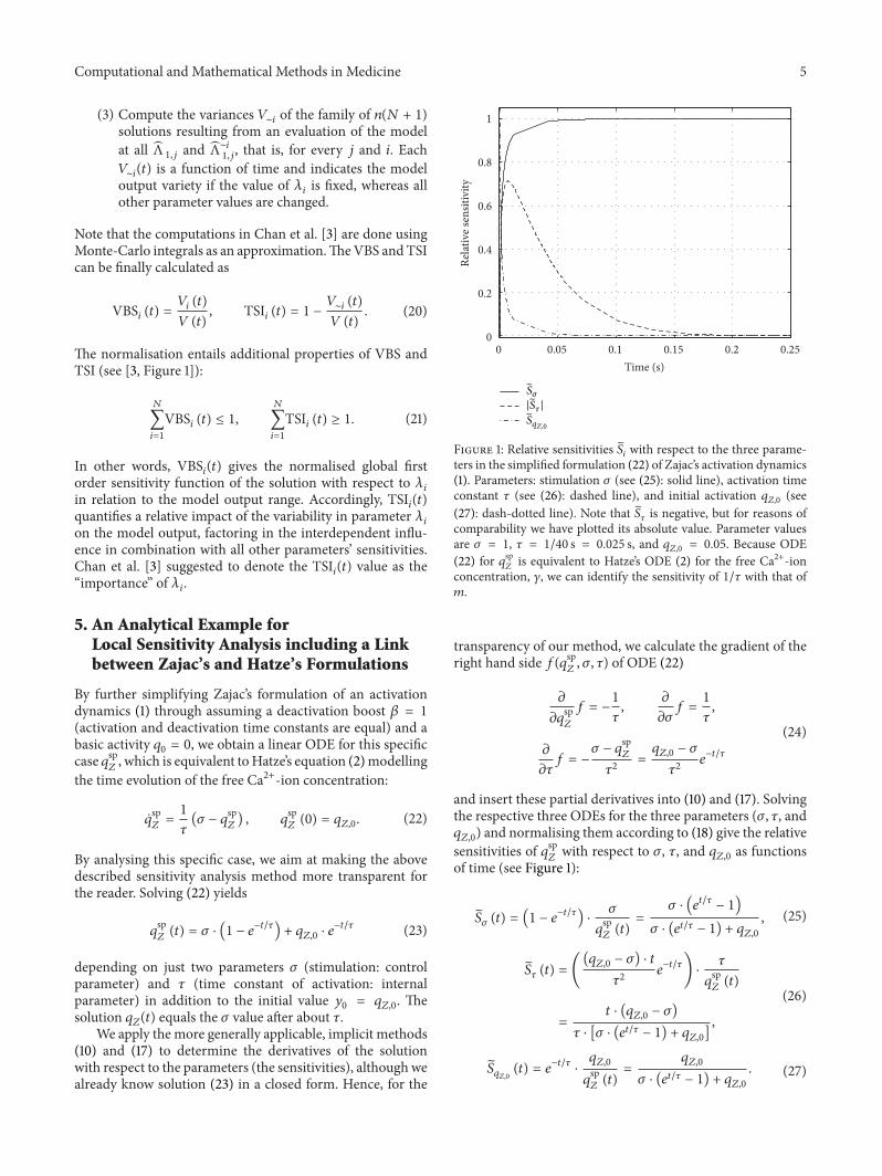
Figure 1: Relative sensitivities 𝑆𝑖

with respect to the three parame-ters in the simplified formulation (22) of Zajac’s activation dynamics(1). Parameters: stimulation 𝜎 (see (25): solid line), activation timeconstant 𝜏 (see (26): dashed line), and initial activation 𝑞

𝑍,0

(see(27): dash-dotted line). Note that 𝑆

𝜏

is negative, but for reasons ofcomparability we have plotted its absolute value. Parameter valuesare 𝜎 = 1, 𝜏 = 1/40 s = 0.025 s, and 𝑞

𝑍,0

= 0.05. Because ODE(22) for 𝑞sp

𝑍

is equivalent to Hatze’s ODE (2) for the free Ca2+-ionconcentration, 𝛾, we can identify the sensitivity of 1/𝜏 with that of𝑚.

transparency of our method, we calculate the gradient of theright hand side 𝑓(𝑞sp

𝑍

, 𝜎, 𝜏) of ODE (22)

𝜕

𝜕𝑞sp𝑍

𝑓 = −1

𝜏,

𝜕

𝜕𝜎𝑓 =1

𝜏,

𝜕

𝜕𝜏𝑓 = −

𝜎 − 𝑞sp𝑍

𝜏2=𝑞𝑍,0

− 𝜎

𝜏2𝑒−𝑡/𝜏

(24)

and insert these partial derivatives into (10) and (17). Solvingthe respective three ODEs for the three parameters (𝜎, 𝜏, and𝑞𝑍,0

) and normalising them according to (18) give the relativesensitivities of 𝑞sp

𝑍

with respect to 𝜎, 𝜏, and 𝑞𝑍,0

as functionsof time (see Figure 1):

𝑆𝜎

(𝑡) = (1 − 𝑒−𝑡/𝜏

) ⋅𝜎

𝑞sp𝑍

(𝑡)=

𝜎 ⋅ (𝑒𝑡/𝜏

− 1)

𝜎 ⋅ (𝑒𝑡/𝜏 − 1) + 𝑞𝑍,0

, (25)

𝑆𝜏

(𝑡) = ((𝑞𝑍,0

− 𝜎) ⋅ 𝑡

𝜏2𝑒−𝑡/𝜏

) ⋅𝜏

𝑞sp𝑍

(𝑡)

=𝑡 ⋅ (𝑞𝑍,0

− 𝜎)

𝜏 ⋅ [𝜎 ⋅ (𝑒𝑡/𝜏 − 1) + 𝑞𝑍,0

],

(26)

𝑆𝑞𝑍,0(𝑡) = 𝑒

−𝑡/𝜏

⋅𝑞𝑍,0

𝑞sp𝑍

(𝑡)=

𝑞𝑍,0

𝜎 ⋅ (𝑒𝑡/𝜏 − 1) + 𝑞𝑍,0

. (27)


A straightforward result is that the time constant 𝜏 has itsmaximum effect on the solution (Figure 1, see 𝑆

𝜏

(𝑡)) at time𝑡 = 𝜏. In case of a step in stimulation, the sensitivity 𝑆

𝜏

(𝑡)

vanishes in the initial situation and exponentially approacheszero again after a few further multiples of the typical period𝜏. Note that 𝑆

𝜏

(𝑡) is negative, which means that an increase in𝜏 decelerates activation.Thus, for a fixed initial value 𝑞

𝑍,0

, thesolution value 𝑞

𝑍

(𝑡) decreases at a given point in time if 𝜏 isincreased. After a step in stimulation 𝜎, the time in which thesolution 𝑞

𝑍

(𝑡) bears some memory of its initial value 𝑞𝑍,0

isequal to the period of being nonsensitive to any further stepin 𝜎 (compare 𝑆

𝑞𝑍,0

(𝑡) to 𝑆𝜎

(𝑡) and (25) to (27)). After about𝜏/2, the sensitivity 𝑆

𝑞𝑍,0

(𝑡) has already fallen to about 0.1 and𝑆𝜎

(𝑡) to about 0.9 accordingly.

6. The Numerical Approach and Results

Typically, biological dynamics are represented by nonlinearODEs. Therefore, the linear ODE used for describing activa-tion dynamics in the Zajac [5] case (1) ismore of an exception.For example, a closed-form solution can be given. Equation(23) is an example as shown in the previous section for thereduced case of nonboosted deactivation (22).

In general, however, nonlinear ODEs used in biome-chanical modelling, as the Hatze [6] case (5) for describingactivation dynamics, can only be solved numerically. It isunderstood that any explicit formulation of a model in termsof ODEs allows providing the partial derivatives of their righthand sides𝑓with respect to themodel parameters in a closedform. Fortunately, this is exactly what is required as part ofthe sensitivity analysis approach presented in Section 3, inparticular in (10).

As an application for applying this approach, we willnow present a comparison of both formulations of activationdynamics.The example indicates that the approachmay be ofgeneral value because it is common practice in biomechanicalmodelling to (i) formulate the ODEs in closed form and (ii)integrate the ODEs numerically. Adding further sensitivityODEs for model parameters then becomes an inexpensiveenhancement of the procedure used to solve the problemanyway.

For the two different activation dynamics [5, 6], theparameter sets Λ

𝑍

and Λ𝐻

, respectively, consist of

Λ𝑍

= {𝑞𝑍,0

, 𝜎, 𝑞0

, 𝜏, 𝛽} , (28)

Λ𝐻

= {𝑞𝐻,0

, 𝜎, 𝑞0

, 𝑚, 𝜌𝑐

, ], ℓ𝜌

, ℓCErel} , (29)

including the initial conditions. The numerical solutionsfor these ODEs were computed within the MATLAB envi-ronment (The MathWorks, Natick, USA; version R2013b),using the preimplemented numerical solver 𝑜𝑑𝑒45 which isa Runge-Kutta algorithm of order 5 (for details see [23]).

6.1. Results for Zajac’s Activation Dynamics: Sensitivity Func-tions. We simulated activation dynamics for the parameterset Λ𝑍

(28) leaving two of the values constant (𝑞0

= 0.005,𝜏 = 1/40 s) and varying the other three (initial condition 𝑞

𝑍,0

,

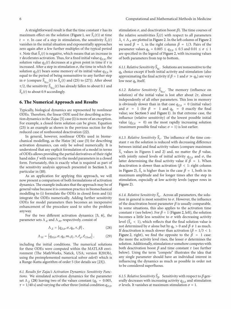
stimulation 𝜎, and deactivation boost 𝛽). The time courses ofthe relative sensitivities 𝑆

𝑖

(𝑡) with respect to all parameters𝜆𝑖

∈ Λ𝑍

are plotted in Figure 2. In the left column of Figure 2we used 𝛽 = 1, in the right column 𝛽 = 1/3. Pairs of theparameter values 𝑞

0

= 0.005 ≤ 𝑞𝑍,0

≤ 0.5 and 0.01 ≤ 𝜎 ≤ 1are specified in the legend of Figure 2, with increasing valuesof both parameters from top to bottom.

6.1.1. Relative Sensitivity 𝑆𝑞0

. Solutions are nonsensitive to the𝑞0

choice except if both initial activity and stimulation (alsoapproximating the final activity if 𝛽 = 1 and 𝜎 ≫ 𝑞

0

) are verylow near 𝑞

0

itself.

6.1.2. Relative Sensitivity 𝑆𝑞𝑍,0

. The memory (influence onsolution) of the initial value is lost after about 2𝜏, almostindependently of all other parameters. This loss in memoryis obviously slower than in that case 𝑞

𝑍,0

= 0 (initial value)and 𝜎 = 1 (for 𝛽 = 1 and 𝑞

0

= 0 exactly the finalvalue; see Section 5 and Figure 1). In that extreme case, theinfluence (relative sensitivity) of the lowest possible initialvalue (𝑞

𝑍,0

= 0) on the most rapidly increasing solution(maximum possible final value: 𝜎 = 1) is lost earlier.

6.1.3. Relative Sensitivity 𝑆𝜏

. The influence of the time con-stant 𝜏 on the solution is reduced with decreasing differencebetween initial and final activity values (compare maximum𝑆𝜏

values in Figures 1 and 2) and, no matter the 𝛽 value,with jointly raised levels of initial activity 𝑞

𝑍,0

and 𝜎, thelatter determining the final activity value if 𝛽 = 1. Whendeactivation is slower than activation (𝛽 < 1: right columnin Figure 2), 𝑆

𝜏

is higher than in the case 𝛽 = 1, both in itsmaximum amplitude and for longer times after the step instimulation, especially at low activity levels (upper rows inFigure 2).

6.1.4. Relative Sensitivity 𝑆𝜎

. Across all parameters, the solu-tion in general is most sensitive to 𝜎. However, the influenceof the deactivation boost parameter 𝛽 is usually comparable.In some situations, this also applies to the activation timeconstant 𝜏 (see below). For 𝛽 = 1 (Figure 2, left), the solutionbecomes a little less sensitive to 𝜎 with decreasing activitylevel (𝑆

𝜎

< 1), which reflects that the final solution value isnot determined by 𝜎 alone but by 𝑞

0

> 0 and 𝛽 = 1 as much.If deactivation is much slower than activation (𝛽 = 1/3 < 1:Figure 2, right), we find the opposite to the 𝛽 = 1 case:the more the activity level rises, the lesser 𝜎 determines thesolution.Additionally, stimulation𝜎 somehow competeswithboth deactivation boost 𝛽 and time constant 𝜏 (see furtherbelow). Using the term “compete” illustrates the idea thatany single parameter should have an individual interest ininfluencing the dynamics as much as possible in order notto be considered superfluous.

6.1.5. Relative Sensitivity 𝑆𝛽

. Sensitivity with respect to𝛽 gen-erally decreases with increasing activity 𝑞

𝑍,0

and stimulation𝜎 levels. It vanishes at maximum stimulation 𝜎 = 1.


𝜏0 0.1 0.2 0.3 0.4 0.5Time (s)

−1

−0.5

0

0.5

1Re

lativ

e sen

sitiv

ity

(a)

0 0.1 0.2 0.3 0.4 0.5Time (s)

𝜏−1

−0.5

0

0.5

1

Rela

tive s

ensit

ivity

𝜏/𝛽

(b)

𝜏0 0.1 0.2 0.3 0.4 0.5Time (s)

−1

−0.5

0

0.5

1

Rela

tive s

ensit

ivity

(c)

0 0.1 0.2 0.3 0.4 0.5Time (s)

𝜏−1

−0.5

0

0.5

1

Rela

tive s

ensit

ivity

𝜏/𝛽

(d)

S𝛽S𝜏

𝜏0 0.1 0.2 0.3 0.4 0.5Time (s)

−1

−0.5

0

0.5

1

Rela

tive s

ensit

ivity

S𝜎

Sq𝑍,0

Sq0

(e)

0 0.1 0.2 0.3 0.4 0.5𝜏−1

−0.5

0

0.5

1

Rela

tive s

ensit

ivity

Time (s)

S𝛽S𝜏

S𝜎

Sq𝑍,0

Sq0

𝜏/𝛽

(f)

Figure 2: Continued.


0 0.1 0.2 0.3 0.4 0.5−1

−0.5

0

0.5

1

Time (s)

Rela

tive s

ensit

ivity

𝜏

S𝛽S𝜏

S𝜎

Sq𝑍,0

Sq0

(g)

0 0.1 0.2 0.3 0.4 0.5−1

−0.5

0

0.5

1

Rela

tive s

ensit

ivity

𝜏

Time (s)

S𝛽S𝜏

S𝜎

Sq𝑍,0

Sq0

𝜏/𝛽

(h)


with respect to all parameters 𝜆𝑖

(set Λ𝑍

(28)) in Zajac’s activation dynamics (1). Parameter values variedfrom top (i) to bottom (iv) row: (i) 𝑞

𝑍,0

= 𝑞0

= 0.005, 𝜎 = 0.01, (ii) 𝑞𝑍,0

= 0.05, 𝜎 = 0.1, (iii) 𝑞𝑍,0

= 0.2, 𝜎 = 0.4, and (iv) 𝑞𝑍,0

= 0.5, 𝜎 = 1; leftcolumn: 𝛽 = 1, right column: 𝛽 = 1/3.

6.1.6. Relative Sensitivities 𝑆𝜎

, 𝑆𝛽

, 𝑆𝜏

. At submaximal stimu-lation levels 𝜎 < 1, the final solution value is determinedto almost the same degree by stimulation 𝜎 and deactivationboost 𝛽, yet with opposite tendencies (𝑆

𝜎

> 0, 𝑆𝛽

< 0).As explained, both parameters compete for their impact onthe final solution value. Only at maximum stimulation 𝜎 =1 (lowest row in Figure 2), this parameter competition isresolved in favour of 𝜎. In this specific case, 𝛽 does notinfluence the solution at all. For 𝛽 = 1 the competition aboutinfluencing the solution is intermittently but only slightlybiased by 𝜏: sensitivity 𝑆

𝜏

peaks at comparably lowmagnitudearound 𝑡 = 𝜏. This 𝜏 influence comes likewise intermittentlyat the cost of 𝛽 influence: the absolute value of 𝑆

𝛽

rises alittle slower than 𝑆

𝜎

. In the case 𝛽 < 1, this competitionbecomes more differentiated and spread out in time. Againat submaximal stimulation and activity levels, the absolutevalue of 𝑆

𝜏

is lower than that of 𝑆𝜎

but higher than thatof 𝑆𝛽

, making all three parameters 𝜎, 𝛽, and 𝜏 compete tocomparable degrees for an impact on the solution until about𝑡 = 4𝜏. Also, 𝑆

𝜏

does not vanish before about 𝑡 = 10𝜏.

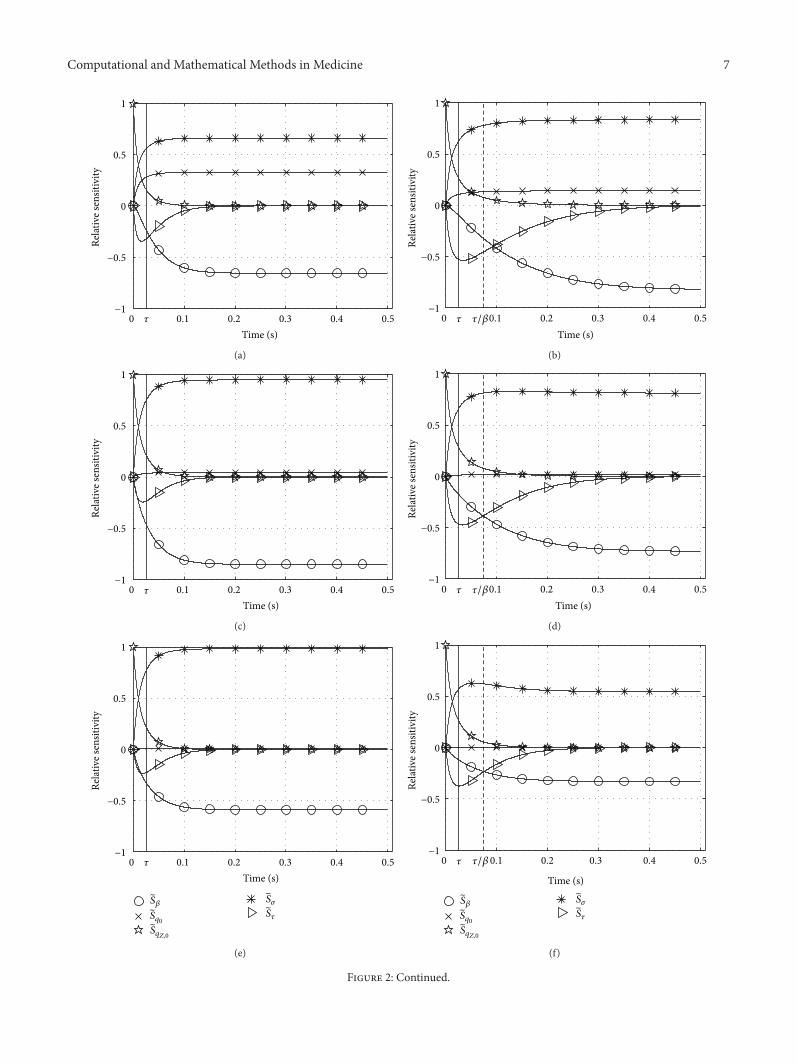
6.2. Results for Hatze’s Activation Dynamics: Sensitivity Func-tions. We also simulated activation dynamics for the param-eter set Λ

𝐻

(29), leaving now four of the values constant(𝑞0

= 0.005, 𝑚 = 10 1/s, ℓ𝜌

= 2.9, ℓCErel = 1) and againvarying three others (initial condition 𝑞

𝑍,0

, stimulation𝜎, andnonlinearity ]), keeping in mind that the eighth parameter(𝜌𝑐

) is assumed to depend on ]. Time courses of the relativesensitivities 𝑆

𝑖

(𝑡) with respect to all parameters 𝜆𝑖

∈ Λ𝐻

areplotted (see Figure 3). In the left column of Figure 3, ] = 2,

𝜌𝑐

= 9.10 is used, in the right column ] = 3, 𝜌𝑐

= 7.24. Here,the same pairs of the parameter values (𝑞

0

= 0.005 ≤ 𝑞𝑍,0

≤

0.5 and 0.01 ≤ 𝜎 ≤ 1, increasing from top to bottom; seelegend of Figure 3) are used as in Section 6.1 (Figure 2).

Hatze’s activation dynamics (5) are nonlinear unlikeZajac’s activation dynamics (1). This nonlinearity manifestsparticularly in a changeful influence of the parameter ].Additionally, the parameter 𝑚 is just roughly comparable tothe inverse of the exponential time constant 𝜏 in Zajac’s linearactivation dynamics.

6.2.1. Relative Sensitivity 𝑆𝑚

. In Zajac’s linear differentialequation (1), 𝜏 establishes a distinct time scale independentof all other parameters.The parameter𝑚 in Hatze’s activationdynamics (5) is just formally equivalent to the reciprocal of 𝜏:the sensitivity 𝑆

𝑚

does not peak stringently at 𝑡 = 1/𝑚 = 0.1 sbut rather diffusely between about 0.05 s and 0.1 s in bothof the cases ] = 2 and ] = 3. At first this is not surprisingbecause the scaling factor in Hatze’s dynamics is ] ⋅ 𝑚 ratherthan just𝑚. However, ] ⋅𝑚 does not fix an invariant time scalefor Hatze’s nonlinear differential equation. This fact becomesparticularly prominent at extremely low activity levels for ] =2 (Figure 3, left, top row) and up to moderately submaximalactivity levels for ] = 3 (Figure 3, right, top two rows). Here,𝑆𝑚

is negative, which means that increasing the parameter𝑚results in less steeply increasing activity. This observation iscounterintuitive to identifying 𝑚 with a reciprocal of a timeconstant like 𝜏. Rather than being expected from the product]⋅𝑚, the exponent ] does not linearly scale the time behaviourbecause 𝑆

𝑚

peaks do not occur systematically earlier in the] = 3 case as compared to ] = 2.


−1

−0.5

0

0.5

1

Rela

tive s

ensit

ivity

0 0.1 0.2 0.3 0.4 0.5Time (s)1

/�m

1/m

(a)

−0.2

0

0.2

0.4

0.6

0.8

1

1.2

Rela

tive s

ensit

ivity

0 0.1 0.2 0.3 0.4 0.5

Time (s)1/�m

1/m

(b)

−3

−2

−1

0

1

2

3

Rela

tive s

ensit

ivity

Time (s)

0 0.1 0.2 0.3 0.4 0.5

1/�m

1/m

(c)

−4

−3

−2

−1

0

1

2

3

Rela

tive s

ensit

ivity

0 0.1 0.2 0.3 0.4 0.5

Time (s)1/�m

1/m

(d)

−0.2

0

0.2

0.4

0.6

0.8

1

1.2

Rela

tive s

ensit

ivity

S𝓁𝜌

S𝜎

SmS�

SqH,0

Sq0

0 0.1 0.2 0.3 0.4 0.5

Time (s)

1/�m

1/m

S𝜌𝑐

S𝓁CE

(e)

−0.5

0

0.5

1

1.5

2

2.5

Rela

tive s

ensit

ivity

S𝓁𝜌

S𝜎

SmS�

SqH,0

Sq0

0 0.1 0.2 0.3 0.4 0.5

Time (s)

1/�m

1/m

S𝜌𝑐

S𝓁CE

(f)

Figure 3: Continued.


0

0.2

0.4

0.6

0.8

1Re

lativ

e sen

sitiv

ity

S𝓁𝜌

S𝜎

SmS�

SqH,0

Sq0

0 0.1 0.2 0.3 0.4 0.5

Time (s)

1/�m

1/m

S𝜌𝑐

S𝓁CE

(g)

0

0.2

0.4

0.6

0.8

1

Rela

tive s

ensit

ivity

0 0.1 0.2 0.3 0.4 0.5

Time (s)

S𝓁𝜌

S𝜎

SmS�

SqH,0

Sq0

S𝜌𝑐

S𝓁CE

1/�m

1/m

(h)


with respect to all parameters 𝜆𝑖

(set Λ𝐻

(29)) in Hatze’s activation dynamics (5). Parameter values variedfrom top (i) to bottom (iv) row: (i) 𝑞

𝐻,0

= 𝑞0

= 0.005, 𝜎 = 0.01, (ii) 𝑞𝐻,0

= 0.05, 𝜎 = 0.1, (iii) 𝑞𝐻,0

= 0.2, 𝜎 = 0.4, and (iv) 𝑞𝐻,0

= 0.5, 𝜎 = 1;left column: ] = 2, 𝜌

𝑐

= 9.10, right column: ] = 3, 𝜌𝑐

= 7.24.

6.2.2. Relative Sensitivity 𝑆𝑞𝐻,0

. Losing the memory of theinitial condition confirms the analysis of time behaviourbased on 𝑆

𝑚

. At high activity levels (Figure 3, bottom row),Hatze’s activation dynamics loses memory at identical timehorizons (nomatter the ] value) seemingly slower for higher ]at intermediate levels (Figure 3, two middle rows) and clearlyfaster at very low levels (Figure 3, top row). The parameter𝑚still does roughly determine the time horizon in which thememory of the initial condition 𝑞

𝐻,0

is lost and the influenceof all other parameters is continuously switched on from zeroinfluence at 𝑡 = 0.

6.2.3. Relative Sensitivity 𝑆𝑞0

. As in Zajac’s dynamics thesolution is generally only sensitive to 𝑞

0

at very low stimu-lation levels 𝜎 ≈ 𝑞

0

(Figure 3, top row). At such levels, the] = 3 case shows the peculiarity that the solution becomesstrikingly insensitive to any other parameter than 𝑞

0

itself(and 𝑞

𝐻,0

). The time evolution of the solution is more orless determined by just this minimum (𝑞

0

) and initial (𝑞𝐻,0

)activities, and𝑚 determining the approximate switching timehorizon between both. The ℓCE dependency, constituting acrucial property of Hatze’s activation dynamics, is practicallysuppressed for ] = 3 at very low activities and stimulations. Incontrast, 𝑆

ℓCErelremains for ] = 2 on a low but still significant

level of about a fourth of the three dominating quantities 𝑆𝑞0

,𝑆𝑞𝐻,0

, and 𝑆].

6.2.4. Relative Sensitivity 𝑆]. The sensitivity with respect to] is extraordinarily high at low activities and stimulationsaround 0.1, both for ] = 2 and for ] = 3 (Figure 3, second

row from top), additionally at extremely low levels for ] = 2(Figure 3, left, top row). At moderately submaximal levels(Figure 3, third row from top), the solution is influenced withan already inverted tendency (𝑆] changes sign to positive)after around a 1/𝑚 time horizon for ] = 2. However, atthese levels the solution is practically insensitive to ] for any]. At high levels (Figure 3, bottom row) we find that there isno change in the character of time evolution of the solution,despite the specific value of ]. The degree of nonlinearity ]is unimportant because the time evolution and the rankingof all other sensitivities are hardly influenced by ]. In bothcases, the rise in activity is quickened by increasing ] (𝑆] > 0),as opposed to low activity and stimulation levels where risesin activity are slowed down (𝑆] < 0; see also above).

6.2.5. Relative Sensitivities 𝑆𝜎

, 𝑆𝜌𝑐

, 𝑆ℓCErel

, and 𝑆ℓ𝜌

. Of all theremaining parameters, stimulation 𝜎, scaled maximum freeCa2+-ion concentration 𝜌

𝑐

, relative CE length ℓCErel, and thepole ℓ

𝜌

of the length dependency inHatze’s activation dynam-ics, the latter has the lowest influence on the solution. Theinfluence characters of all four parameters are yet completelyidentical. Their sensitivities are always positive and coupledby fixed scaling ratios due to all of them occurring within justone product on the right side of (5). 𝑆

𝜎

and 𝑆𝜌𝑐

are identical,while the sensitivity with respect to ℓCErel is the highest, withratios 𝑆

ℓCErel/𝑆ℓ𝜌

≈ 3 and 𝑆ℓCErel/𝑆𝜎

≈ 1.2. Except at very lowactivity (where 𝑞

0

plays a dominating role) and except for thegenerally changeful ] influence, these are the four parametersthat dominate the solution after an initial phase in which theinitial activity 𝑞

𝐻,0

determines its evolution. The parameter


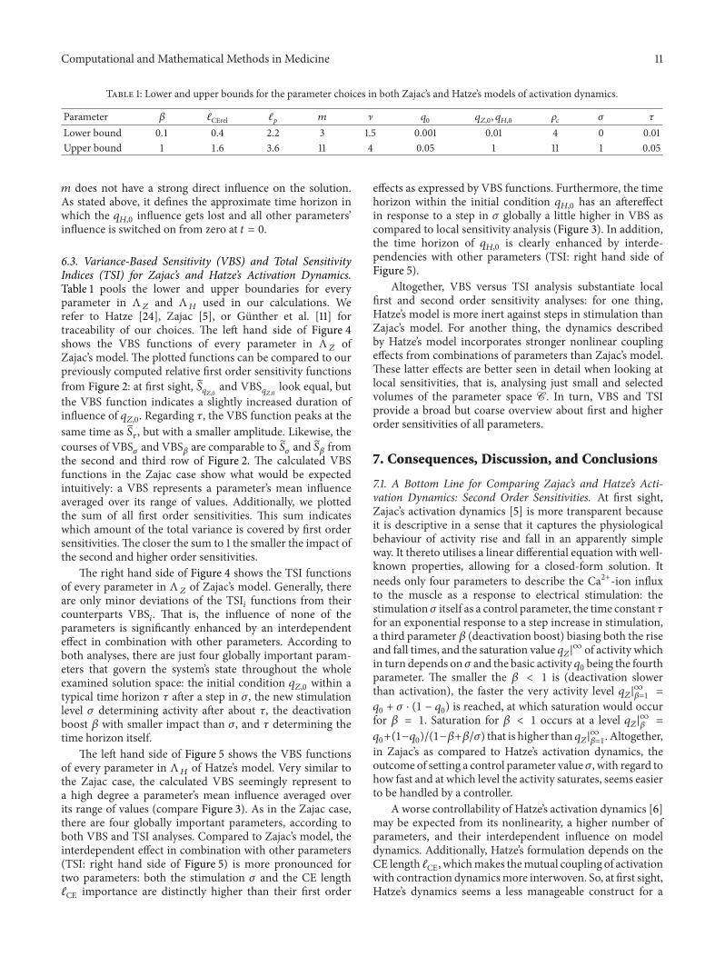
Table 1: Lower and upper bounds for the parameter choices in both Zajac’s and Hatze’s models of activation dynamics.

Parameter 𝛽 ℓCErel ℓ𝑝

𝑚 ] 𝑞0

𝑞𝑍,0

, 𝑞𝐻,0

𝜌𝑐

𝜎 𝜏

Lower bound 0.1 0.4 2.2 3 1.5 0.001 0.01 4 0 0.01Upper bound 1 1.6 3.6 11 4 0.05 1 11 1 0.05

𝑚 does not have a strong direct influence on the solution.As stated above, it defines the approximate time horizon inwhich the 𝑞

𝐻,0

influence gets lost and all other parameters’influence is switched on from zero at 𝑡 = 0.

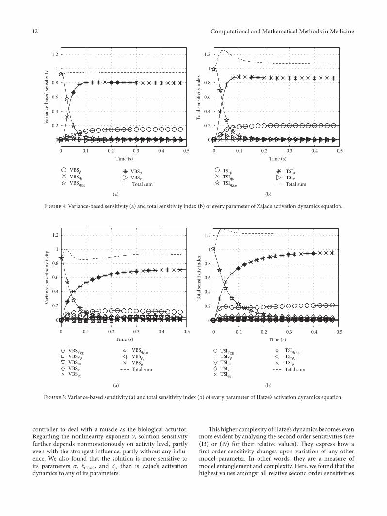
6.3. Variance-Based Sensitivity (VBS) and Total SensitivityIndices (TSI) for Zajac’s and Hatze’s Activation Dynamics.Table 1 pools the lower and upper boundaries for everyparameter in Λ

𝑍

and Λ𝐻

used in our calculations. Werefer to Hatze [24], Zajac [5], or Gunther et al. [11] fortraceability of our choices. The left hand side of Figure 4shows the VBS functions of every parameter in Λ

𝑍

ofZajac’s model. The plotted functions can be compared to ourpreviously computed relative first order sensitivity functionsfrom Figure 2: at first sight, 𝑆

𝑞𝑍,0

and VBS𝑞𝑍,0

look equal, butthe VBS function indicates a slightly increased duration ofinfluence of 𝑞

𝑍,0

. Regarding 𝜏, the VBS function peaks at thesame time as 𝑆

𝜏

, but with a smaller amplitude. Likewise, thecourses of VBS

𝜎

and VBS𝛽

are comparable to 𝑆𝜎

and 𝑆𝛽

fromthe second and third row of Figure 2. The calculated VBSfunctions in the Zajac case show what would be expectedintuitively: a VBS represents a parameter’s mean influenceaveraged over its range of values. Additionally, we plottedthe sum of all first order sensitivities. This sum indicateswhich amount of the total variance is covered by first ordersensitivities.The closer the sum to 1 the smaller the impact ofthe second and higher order sensitivities.

The right hand side of Figure 4 shows the TSI functionsof every parameter in Λ

𝑍

of Zajac’s model. Generally, thereare only minor deviations of the TSI

𝑖

functions from theircounterparts VBS

𝑖

. That is, the influence of none of theparameters is significantly enhanced by an interdependenteffect in combination with other parameters. According toboth analyses, there are just four globally important param-eters that govern the system’s state throughout the wholeexamined solution space: the initial condition 𝑞

𝑍,0

within atypical time horizon 𝜏 after a step in 𝜎, the new stimulationlevel 𝜎 determining activity after about 𝜏, the deactivationboost 𝛽 with smaller impact than 𝜎, and 𝜏 determining thetime horizon itself.

The left hand side of Figure 5 shows the VBS functionsof every parameter in Λ

𝐻

of Hatze’s model. Very similar tothe Zajac case, the calculated VBS seemingly represent toa high degree a parameter’s mean influence averaged overits range of values (compare Figure 3). As in the Zajac case,there are four globally important parameters, according toboth VBS and TSI analyses. Compared to Zajac’s model, theinterdependent effect in combination with other parameters(TSI: right hand side of Figure 5) is more pronounced fortwo parameters: both the stimulation 𝜎 and the CE lengthℓCE importance are distinctly higher than their first order

effects as expressed by VBS functions. Furthermore, the timehorizon within the initial condition 𝑞

𝐻,0

has an aftereffectin response to a step in 𝜎 globally a little higher in VBS ascompared to local sensitivity analysis (Figure 3). In addition,the time horizon of 𝑞

𝐻,0

is clearly enhanced by interde-pendencies with other parameters (TSI: right hand side ofFigure 5).

Altogether, VBS versus TSI analysis substantiate localfirst and second order sensitivity analyses: for one thing,Hatze’s model is more inert against steps in stimulation thanZajac’s model. For another thing, the dynamics describedby Hatze’s model incorporates stronger nonlinear couplingeffects from combinations of parameters than Zajac’s model.These latter effects are better seen in detail when looking atlocal sensitivities, that is, analysing just small and selectedvolumes of the parameter space C. In turn, VBS and TSIprovide a broad but coarse overview about first and higherorder sensitivities of all parameters.

7. Consequences, Discussion, and Conclusions

7.1. A Bottom Line for Comparing Zajac’s and Hatze’s Acti-vation Dynamics: Second Order Sensitivities. At first sight,Zajac’s activation dynamics [5] is more transparent becauseit is descriptive in a sense that it captures the physiologicalbehaviour of activity rise and fall in an apparently simpleway. It thereto utilises a linear differential equation with well-known properties, allowing for a closed-form solution. Itneeds only four parameters to describe the Ca2+-ion influxto the muscle as a response to electrical stimulation: thestimulation𝜎 itself as a control parameter, the time constant 𝜏for an exponential response to a step increase in stimulation,a third parameter 𝛽 (deactivation boost) biasing both the riseand fall times, and the saturation value 𝑞

𝑍

|∞ of activity which

in turn depends on𝜎 and the basic activity 𝑞0

being the fourthparameter. The smaller the 𝛽 < 1 is (deactivation slowerthan activation), the faster the very activity level 𝑞

𝑍

|∞

𝛽=1

=

𝑞0

+ 𝜎 ⋅ (1 − 𝑞0

) is reached, at which saturation would occurfor 𝛽 = 1. Saturation for 𝛽 < 1 occurs at a level 𝑞

𝑍

|∞

𝛽

=

𝑞0

+(1−𝑞0

)/(1−𝛽+𝛽/𝜎) that is higher than 𝑞𝑍

|∞

𝛽=1

. Altogether,in Zajac’s as compared to Hatze’s activation dynamics, theoutcome of setting a control parameter value𝜎, with regard tohow fast and at which level the activity saturates, seems easierto be handled by a controller.

A worse controllability of Hatze’s activation dynamics [6]may be expected from its nonlinearity, a higher number ofparameters, and their interdependent influence on modeldynamics. Additionally, Hatze’s formulation depends on theCE length ℓCE, whichmakes themutual coupling of activationwith contraction dynamicsmore interwoven. So, at first sight,Hatze’s dynamics seems a less manageable construct for a


0 0.1 0.2 0.3 0.4 0.5

0

0.2

0.4

0.6

0.8

1

1.2

Time (s)

Varia

nce-

base

d se

nsiti

vity

Total sum

𝜎

𝜏

𝛽VBS VBSVBSVBSq0

VBSq𝑍,0

(a)

0

0.2

0.4

0.6

0.8

1

1.2

Tota

l sen

sitiv

ity in

dex

0 0.1 0.2 0.3 0.4 0.5Time (s)

Total sum

TSI𝜎TSI𝜏

TSI𝛽TSIq0TSIq𝑍,0

(b)

Figure 4: Variance-based sensitivity (a) and total sensitivity index (b) of every parameter of Zajac’s activation dynamics equation.

0

0.2

0.4

0.6

0.8

1

1.2

Varia

nce-

base

d se

nsiti

vity

0 0.1 0.2 0.3 0.4 0.5Time (s)

Total sum

VBSVBSVBSm

VBS

VBS𝜎

VBSVBS

VBS�

𝓁p

qH,0

𝜌𝑐

𝓁CE

q0

(a)

0

0.2

0.4

0.6

0.8

1

1.2

Tota

l sen

sitiv

ity in

dex

0 0.1 0.2 0.3 0.4 0.5Time (s)

Total sum

TSI TSITSI

𝜎TSITSI

mTSI�TSI

TSI

𝓁p

qH,0

q0

𝜌𝑐

𝓁CE

(b)

Figure 5: Variance-based sensitivity (a) and total sensitivity index (b) of every parameter of Hatze’s activation dynamics equation.

controller to deal with a muscle as the biological actuator.Regarding the nonlinearity exponent ], solution sensitivityfurther depends nonmonotonously on activity level, partlyeven with the strongest influence, partly without any influ-ence. We also found that the solution is more sensitive toits parameters 𝜎, ℓCErel, and ℓ𝜌 than is Zajac’s activationdynamics to any of its parameters.

This higher complexity ofHatze’s dynamics becomes evenmore evident by analysing the second order sensitivities (see(13) or (19) for their relative values). They express how afirst order sensitivity changes upon variation of any othermodel parameter. In other words, they are a measure ofmodel entanglement and complexity. Here, we found that thehighest values amongst all relative second order sensitivities


in Zajac’s activation dynamics are about −0.8 (��𝛽𝜎

) and 1.6(��𝛽𝛽

). In Hatze’s activation dynamics, the highest relativesecond order sensitivities are those with respect to ] orℓCErel (in particular for 𝜎, 𝜌

𝑐

, and ], ℓCErel themselves) withmaximum values between about −8.0 (��

ℓCErel], ��]𝜌𝑐) and 13.4(��ℓCErelℓCErel

, ��ℓCErel𝜌𝑐

, ��ℓCErel𝜎

, ��]] at submaximal activity). Thatis, they are an order of magnitude higher than in Zajac’sactivation dynamics.

Yet, we have to acknowledge that Hatze’s activationdynamics contains crucial physiological features that gobeyond Zajac’s description.

7.2. A Plus for Hatze’s Approach: Length Dependency. It hasbeen established that the length dependency of activationdynamics is both physiological [7] and functionally vital[15] because it largely contributes to low-frequency musclestiffness. It has also been verified that Hatze’s model approachprovides a good approximation for experimental data [7]. Inthat study, ] = 3 was used without comparing to the ] = 2case. There seem to be arguments in favour of ] = 2 from amathematical point of view. In particular, the less changefulscaling of the activation dynamics’ characteristics down tovery low activity and stimulation levels, at which some CElength sensitivity remains, seem to be an advantage whencompared to the ] = 3 case. Up to this point, we have arguedsolelymathematically. It is, however, physiological reality thatis eventually aimed at. We therefore repeated the model fitdone by Kistemaker et al. [7] while now allowing a variationin ] and in force-length relations.

7.3. AnOptimal Parameter Set for Hatze’s ActivationDynamicsPlus CEForce-Length Relation. Sensitivity analysis allows rat-ing Hatze’s approach as an entangled construct. Additionally,Kistemaker et al. [7] decided to choose ] = 3 without givinga reason for discarding ] = 2. It further seemed that theydid not perform an algorithmic optimisation across varioussubmaximal stimulation levels to find a muscle parameterset, which best fits known shifts ΔℓCE,opt,submax = ℓCE,opt −ℓCE,opt,submax in optimal, submaximal CE length ℓCE,opt,submaxat which isometric force 𝐹isom = 𝐹isom(𝑞, ℓCE) peaks. Accord-ingly, it seemed worth performing such an optimisationbecause 𝐹isom generally depends on length ℓCE and activity 𝑞,and the lattermay be additionally biased by an ℓCE-dependentcapability for building up cross-bridges at a given level 𝛾 offree Ca2+-ions in the sarcoplasma, as formulated in Hatze’sapproach: 𝐹isom(𝑞, ℓCE) = 𝐹max ⋅ 𝑞(𝛾, ℓCE) ⋅ 𝐹ℓ(ℓCE). Thus, ashift in optimal CE length ΔℓCE,opt,submax with changing 𝛾 canoccur depending on the specific choices of both the lengthdependency of activation 𝑞(𝛾, ℓCE) (see (3) and (4)) and theCE’s force-length relation 𝐹

ℓ

(ℓCE).Consequently, we searched for optimal parameter sets

of Hatze’s activation dynamics in combination with twodifferent force-length relations 𝐹

ℓ

(ℓCE): either a parabola [7]or bell-shaped curves [11, 25]. For a given optimal CE lengthℓCE,opt = 14.8mm [26] representing a rat gastrocnemiusmuscle and three fixed exponent values ] = 2, 3, 4 inHatze’s activation dynamics (all other parameters as given inSection 2), we thus determined Hatze’s constant 𝜌

0

and the

width parameters of the two different force-length relations𝐹ℓ

(ℓCE) (WIDTH in Kistemaker et al. [7] and van Soest andBobbert [9] and Δ𝑊asc = Δ𝑊des = Δ𝑊 in Morl et al. [25],resp.) by an optimisation approach.The objective function tobe minimised was the sum of squared differences betweenthe ΔℓCE,opt,submax values as predicted by the model and asderived from experiments (see Table 2 in Kistemaker et al.[7]) over five stimulation levels𝜎 = 0.55, 0.28, 0.22, 0.17, 0.08.Note that 𝛾 = 𝜎 applies in the isometric situation (see (2)and compare (3)). Further note that experimental data formuscle contractions at very low stimulation levels aremissingin the literature so far: the lowest analysed level available forKistemaker et al. [7] was 𝜎 = 0.08, that is, comparable to thesecond rows from top in Figures 2 and 3.

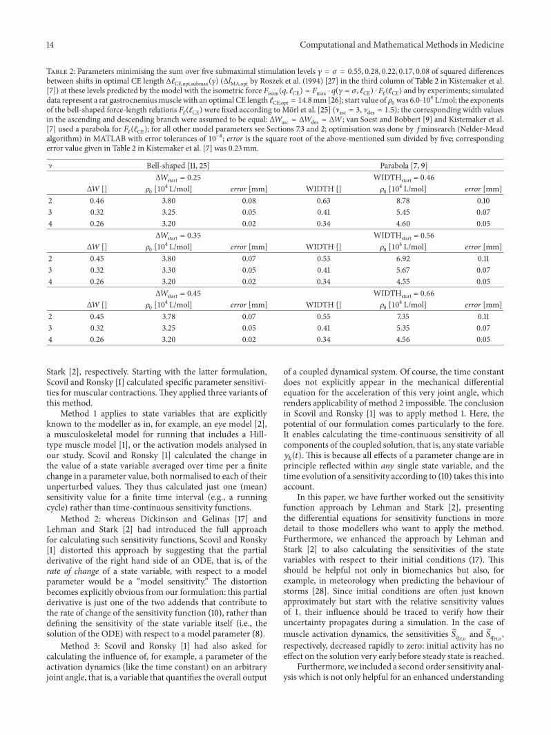
The optimisation results are summarised in Table 2. Thehigher the ] value, the smaller the optimisation error. Thepredictedwidth valuesWIDTHorΔ𝑊, respectively, decreasealong with the error. We would yet tend to exclude the case] = 4 because the predicted width values seem unrealisticallylow when compared to published values from other sources(e.g., WIDTH = 0.56 [9], Δ𝑊 = 0.35 [25]). Furthermore,𝜌0

decreases with ] using the parabola model for 𝐹ℓ

(ℓCE)whereas it saturates between ] = 3 and ] = 4 for thebell-shaped model. The bell-shaped model shows the mostrealistic Δ𝑊 in the case ] = 3 (Δ𝑊 = 0.32). Fitting the samemodel to other contraction modes of the muscle [25], a valueof Δ𝑊 = 0.32 had been found. In contrast, when using theparabola model, realistic WIDTH values between 0.5 and 0.6are predicted by our optimisation for ] = 2.

When comparing the optimised parameter values acrossall start values of the 𝐹

ℓ

(ℓCE) widths, across all ] values,and across both 𝐹

ℓ

(ℓCE) model functions, we find that theresulting optimal parameter sets are more consistent for bell-shaped 𝐹

ℓ

(ℓCE) than for the parabola function. The bell-shaped force-length relation gives generally a better fit. Foreach single ] value, the corresponding optimisation error issmaller when comparing realistic, published WIDTH andΔ𝑊 values that may correspond to each other (WIDTH =0.56 [9] and Δ𝑊 = 0.35 [25]). Additionally, the errorvalues from our optimisation are generally smaller than thecorresponding value calculated from Table 2 in Kistemakeret al. [7] (0.23mm).

In a nutshell, we would say that the most realistic modelfor the isometric force 𝐹isom at submaximal activity levels isthe combination of Hatze’s approach for activation dynamicswith ] = 3 and a bell-shaped curve for the force-lengthrelation 𝐹

ℓ

(ℓCE) with ]asc = 3. As a side effect, we predictthat the parameter value 𝜌

0

, being a weighting factor of thefirst addend in the compact formulation of Hatze’s activationdynamics (5), should be reduced by about 40% (𝜌

0

= 3.25 ⋅

104 L/mol) as compared to the value originally published in

Hatze [13] (𝜌0

= 5.27 ⋅ 104 L/mol).

7.4. A Generalised Method for Calculating Parameter Sen-sitivities. The findings in the last section were initiated bythoroughly comparing twodifferent biomechanicalmodels ofmuscular activation using a systematic sensitivity analysis asintroduced in Dickinson and Gelinas [17] and Lehman and


Table 2: Parameters minimising the sum over five submaximal stimulation levels 𝛾 = 𝜎 = 0.55, 0.28, 0.22, 0.17, 0.08 of squared differencesbetween shifts in optimal CE length ΔℓCE,opt,submax(𝛾) (Δ𝑙MA,opt by Roszek et al. (1994) [27] in the third column of Table 2 in Kistemaker et al.[7]) at these levels predicted by the model with the isometric force 𝐹isom(𝑞, ℓCE) = 𝐹max ⋅ 𝑞(𝛾 = 𝜎, ℓCE) ⋅ 𝐹ℓ(ℓCE) and by experiments; simulateddata represent a rat gastrocnemiusmuscle with an optimal CE length ℓCE,opt = 14.8mm[26]; start value of 𝜌

0

was 6.0⋅104 L/mol; the exponentsof the bell-shaped force-length relations 𝐹

ℓ

(ℓCE) were fixed according to Morl et al. [25] (]asc = 3, ]des = 1.5); the corresponding width valuesin the ascending and descending branch were assumed to be equal: Δ𝑊asc = Δ𝑊des = Δ𝑊; van Soest and Bobbert [9] and Kistemaker et al.[7] used a parabola for 𝐹

ℓ

(ℓCE); for all other model parameters see Sections 7.3 and 2; optimisation was done by 𝑓minsearch (Nelder-Meadalgorithm) in MATLAB with error tolerances of 10−8; error is the square root of the above-mentioned sum divided by five; correspondingerror value given in Table 2 in Kistemaker et al. [7] was 0.23mm.

] Bell-shaped [11, 25] Parabola [7, 9]Δ𝑊start = 0.25 WIDTHstart = 0.46

Δ𝑊[] 𝜌0

[104 L/mol] error [mm] WIDTH [] 𝜌0

[104 L/mol] error [mm]2 0.46 3.80 0.08 0.63 8.78 0.103 0.32 3.25 0.05 0.41 5.45 0.074 0.26 3.20 0.02 0.34 4.60 0.05

Δ𝑊start = 0.35 WIDTHstart = 0.56Δ𝑊[] 𝜌

0


[104 L/mol] error [mm]2 0.45 3.80 0.07 0.53 6.92 0.113 0.32 3.30 0.05 0.41 5.67 0.074 0.26 3.20 0.02 0.34 4.55 0.05

Δ𝑊start = 0.45 WIDTHstart = 0.66Δ𝑊[] 𝜌

0


[104 L/mol] error [mm]2 0.45 3.78 0.07 0.55 7.35 0.113 0.32 3.25 0.05 0.41 5.35 0.074 0.26 3.20 0.02 0.34 4.56 0.05

Stark [2], respectively. Starting with the latter formulation,Scovil and Ronsky [1] calculated specific parameter sensitivi-ties for muscular contractions. They applied three variants ofthis method.

Method 1 applies to state variables that are explicitlyknown to the modeller as in, for example, an eye model [2],a musculoskeletal model for running that includes a Hill-type muscle model [1], or the activation models analysed inour study. Scovil and Ronsky [1] calculated the change inthe value of a state variable averaged over time per a finitechange in a parameter value, both normalised to each of theirunperturbed values. They thus calculated just one (mean)sensitivity value for a finite time interval (e.g., a runningcycle) rather than time-continuous sensitivity functions.

Method 2: whereas Dickinson and Gelinas [17] andLehman and Stark [2] had introduced the full approachfor calculating such sensitivity functions, Scovil and Ronsky[1] distorted this approach by suggesting that the partialderivative of the right hand side of an ODE, that is, of therate of change of a state variable, with respect to a modelparameter would be a “model sensitivity.” The distortionbecomes explicitly obvious from our formulation: this partialderivative is just one of the two addends that contribute tothe rate of change of the sensitivity function (10), rather thandefining the sensitivity of the state variable itself (i.e., thesolution of the ODE) with respect to a model parameter (8).

Method 3: Scovil and Ronsky [1] had also asked forcalculating the influence of, for example, a parameter of theactivation dynamics (like the time constant) on an arbitraryjoint angle, that is, a variable that quantifies the overall output

of a coupled dynamical system. Of course, the time constantdoes not explicitly appear in the mechanical differentialequation for the acceleration of this very joint angle, whichrenders applicability of method 2 impossible. The conclusionin Scovil and Ronsky [1] was to apply method 1. Here, thepotential of our formulation comes particularly to the fore.It enables calculating the time-continuous sensitivity of allcomponents of the coupled solution, that is, any state variable𝑦𝑘

(𝑡). This is because all effects of a parameter change are inprinciple reflected within any single state variable, and thetime evolution of a sensitivity according to (10) takes this intoaccount.

In this paper, we have further worked out the sensitivityfunction approach by Lehman and Stark [2], presentingthe differential equations for sensitivity functions in moredetail to those modellers who want to apply the method.Furthermore, we enhanced the approach by Lehman andStark [2] to also calculating the sensitivities of the statevariables with respect to their initial conditions (17). Thisshould be helpful not only in biomechanics but also, forexample, in meteorology when predicting the behaviour ofstorms [28]. Since initial conditions are often just knownapproximately but start with the relative sensitivity valuesof 1, their influence should be traced to verify how theiruncertainty propagates during a simulation. In the case ofmuscle activation dynamics, the sensitivities 𝑆

𝑞𝑍,0

and 𝑆𝑞𝐻,0

,respectively, decreased rapidly to zero: initial activity has noeffect on the solution very early before steady state is reached.

Furthermore, we included a second order sensitivity anal-ysis which is not only helpful for an enhanced understanding


of the parameter influence but also part of mathematicaloptimisation techniques [29]. The values of ��

𝑖𝑗𝑘

could beinterpreted either as the relative sensitivity of the sensitivity𝑆𝑖𝑘

with respect to another parameter 𝜆𝑗

(and vice versa:𝑆𝑗𝑘

with respect to 𝜆𝑖

) or as the curvature of the graphof the solution 𝑦

𝑘

(𝑡) in the 𝑁 + 𝑀-dimensional solution-parameter space. The latter may help to connect the resultsto the field of mathematical optimisation in which thesecond derivative (Hessian) of a function is often included inobjective functions to find optimal parameter sets.

7.5. Insights into Global Methods. Some additional conclu-sions can be drawn from global sensitivity analysis, inparticular from comparing results in Section 6.3 to thosebased on local sensitivity analysis (Sections 6.1, 6.2, and 7.1).

For Zajac’s activation dynamics, global analysis confirmslocal analysis in stating that there are no significant secondor higher order sensitivities, with the slight exception of thephase of rapid change in activity after a step in stimulation.An experimenter who wants to measure the activation timeconstant 𝜏 can exclude influence from potentially slowerdeactivation processes (𝛽 < 1) by starting from high activitylevels (Figure 2, bottom). It should yet be kept in mind thatbuild-up of activity to the new level is not solely determinedby 𝜏 but might be biased by other parameters than 𝜏 becauseTSI𝜏

peaks during the build-up phase (Figure 4, right).In Hatze’s activation dynamics, the higher order sensi-

tivities play a clearly more significant role, even in the near-steady-state case (Figure 5: stronger deviation from 1 of bothVBS and TSI). When arguing in terms of controllabilityof the models in Section 7.1, we speculated that Zajac’sdynamics might be easier to control than Hatze’s dynamics.Notwithstanding, Figure 5 shows that the stimulation is themost important control factor with even a higher importancethan in Zajac’s formulation.

At first sight unapparent, another result is the importanceof𝜌𝑐

. Froma strictly local point of viewwe concluded that thisparameter should have the same sensitivity as 𝜎 since theyboth are formally equivalent multipliers in Hatze’s ODE (seerelative sensitivities in Figure 3). However, the importanceof 𝜌𝑐

is significantly smaller than that of 𝜎, in fact almostnegligible. Their different global variabilities of values cangive an explanation. The parameter 𝜌

𝑐

in the product 𝜌𝑐

⋅

𝜎 ∈ [4; 11] × [0; 1] has a clearly lower relative variabilitythan 𝜎, measured in maximum percentage deviation fromthe respective mean value. The parameter 𝜌

𝑐

thus acts as anamplifier for 𝜎. Similarly, the parameter ] has a relativelysmall variability throughout the literature. So, although itsdifferential sensitivity is quite large, ] is found to have a lowimportance for the model output. For the latter fact there isyet another reason. In Section 6.2, we have emphasised that] has a very changeful influence on solutions, depending onactivity level. Additionally, its influence is highly dependenton other parameters like length ℓCE and 𝜌

𝑐

(see end ofSection 7.1). Its strong influence in some situations andconfigurations is thus hidden by global averaging.

This demonstrates that the findings of global sensitivityanalysis must be treated with caution because the whole

dynamics of a system is condensed to a single averagefunction per whole parameter range. Without local analysesof the solution space as exemplified in Sections 6.1 and 6.2crucial features of its topology might be lost when solelyrelying on global analysis.

Symbols

ℓCE: Contractile element (CE) length; value:time-depending

ℓCE: Contraction velocity; value: first timederivative of ℓCE

ℓCE,opt: Optimal CE length; value: muscle-specificℓCErel: Relative CE length; value:

ℓCErel = ℓCE/ℓCE,opt (dimensionless)𝐹max: Maximum isometric force of the CE;

value: muscle-specific𝜎: Neural muscle stimulation; value:

time-depending; here: a fixed parameter𝑞: Muscle activity (bound

Ca2+-concentration); value:time-depending

𝑞0

: Basic activity according to Hatze [13];value: 0.005

𝑞𝐻

: Activity according to Hatze [6]; value:time-length-depending

𝑞𝐻,0

: Initial condition for Hatze’s activationODE; value: mutable

𝑞𝑍

: Activity according to Zajac [5]; value:time-depending

𝑞𝑍,0

: Initial condition for Zajac’s activationODE; value: mutable

𝜏: Activation time constant in Zajac [5];value: here: 1/40 s

𝜏deact: Deactivation time constant in Zajac [5];value: here: 1/40 s or 3/40 s

𝛽: Corresponding deactivation boost [5];value: 𝛽 = 𝜏/𝜏deact

]: Exponent in Hatze’s formulation; value: 2or 3

𝑚: Activation frequency constant in Hatze[6]; value: range: 3.67, . . . , 11.25 (1/s); here:10 (1/s)

𝑐: Maximal Ca2+-concentration in Hatze[24]; value: 1.37 ⋅ 10−4mol/L

𝛾: Representation of free Ca2+-concentration[6, 13]; value: time-depending

𝜌: Length dependency of Hatze [24]activation dynamics; value:𝜌(ℓCErel) = 𝜌𝑐 ⋅ ((ℓ𝜌 − 1)/(ℓ𝜌/ℓCErel − 1))

ℓ𝜌

: Pole in Hatze’s length dependencyfunction; value: 2.9

𝜌0

: Factor in van Soest [8], Hatze [6]; value:6.62 ⋅ 10

4 L/mol (] = 2) or 5.27 ⋅ 104 L/mol(] = 3)

𝜌𝑐

: Merging of 𝜌0

and 𝑐; value: 𝜌𝑐

= 𝜌0

⋅ 𝑐;here: 9.10 (] = 2) or 7.24 (] = 3)

Λ: Model parameter set; value:Λ = {𝜆

1

, . . . , 𝜆𝑛

}.


Conflict of Interests

The authors declare that there is no conflict of interestsregarding the publication of this paper.

Acknowledgments

Michael Gunther was supported by “BerufsgenossenschaftNahrungsmittel und Gastgewerbe, Geschaftsbereich Praven-tion, Mannheim” (BGN) and Deutsche Forschungsgemein-schaft (DFG: SCHM2392/5-1), both granted to Syn Schmitt.

References

[1] C. Y. Scovil and J. L. Ronsky, “Sensitivity of a Hill-basedmuscle model to perturbations in model parameters,” Journalof Biomechanics, vol. 39, no. 11, pp. 2055–2063, 2006.

[2] S. L. Lehman and L.W. Stark, “Three algorithms for interpretingmodels consisting of ordinary differential equations: sensitivitycoefficients, sensitivity functions, global optimization,” Mathe-matical Biosciences, vol. 62, no. 1, pp. 107–122, 1982.

[3] K. Chan, A. Saltelli, and S. Tarantola, “Sensitivity analysis ofmodel output: variance-based methods make the difference,” inProceedings of the 29th Conference on Winter Simulation (WSC’97), S. Andradottir, K. Healy, D. Withers, and B. Nelson, Eds.,pp. 261–268, IEEE Computer Society, Washington, DC, USA,1997.

[4] A. Saltelli and K. S. E. Chan, Sensitivity Analysis, John Wiley &Sons, New York, NY, USA, 1st edition, 2000.

[5] F. E. Zajac, “Muscle and tendon: properties, models, scaling,and application to biomechanics and motor control,” CriticalReviews in Biomedical Engineering, vol. 17, no. 4, pp. 359–411,1989.

[6] H. Hatze, “A myocybernetic control model of skeletal muscle,”Biological Cybernetics, vol. 25, no. 2, pp. 103–119, 1977.

[7] D. A. Kistemaker, A. J. van Soest, and M. F. Bobbert, “Length-dependent [Ca2+] sensitivity adds stiffness to muscle,” Journalof Biomechanics, vol. 38, no. 9, pp. 1816–1821, 2005.

[8] A. van Soest, Jumping from structure to control: a simulationstudy of explosive movements [Ph.D. thesis], Vrije Universiteit,Amsterdam, The Netherlands, 1992.

[9] A. J. van Soest and M. F. Bobbert, “The contribution of muscleproperties in the control of explosive movements,” BiologicalCybernetics, vol. 69, no. 3, pp. 195–204, 1993.

[10] G. Cole, A. van den Bogert, A. W. Herzog, and K. Gerritsen,“Modelling of force production in skeletal muscle undergoingstretch,” Journal of Biomechanics, vol. 29, pp. 1091–1104, 1996.

[11] M. Gunther, S. Schmitt, and V. Wank, “High-frequency oscilla-tions as a consequence of neglected serial damping in Hill-typemuscle models,” Biological Cybernetics, vol. 97, no. 1, pp. 63–79,2007.

[12] D. F. B.Haeufle,M.Gunther, A. Bayer, and S. Schmitt, “Hill-typemuscle model with serial damping and eccentric force-velocityrelation,” Journal of Biomechanics, vol. 47, no. 6, pp. 1531–1536,2014.

[13] H. Hatze, Myocybernetic Control Models of Skeletal Muscle,University of South Africa, 1981.

[14] D. A. Kistemaker, A. J. van Soest, and M. F. Bobbert, “Isequilibrium point control feasible for fast goal-directed single-joint movements?” Journal of Neurophysiology, vol. 95, no. 5, pp.2898–2912, 2006.

[15] D. A. Kistemaker, A. J. van Soest, and M. F. Bobbert, “A modelof open-loop control of equilibrium position and stiffness of thehuman elbow joint,” Biological Cybernetics, vol. 96, no. 3, pp.341–350, 2007.

[16] R. T.M. Vukobratovic,General SensitivityTheory, Elsevier, NewYork, NY, USA, 1962.

[17] R. P. Dickinson and R. J. Gelinas, “Sensitivity analysis of ordi-nary differential equation systems—a direct method,” Journal ofComputational Physics, vol. 21, no. 2, pp. 123–143, 1976.

[18] H. ZivariPiran, Efficient simulation, accurate sensitivity analysisand reliable parameter estimation for delay differential equations[Ph.D. thesis], University of Toronto, Toronto, Canada, 2009.

[19] B. W. Bader and T. G. Kolda, “Algorithm 862: matlab tensorclasses for fast algorithm prototyping,” ACM Transactions onMathematical Software, vol. 32, no. 4, pp. 635–653, 2006.

[20] O. Scherzer, Mathematische Modellierung—Vorlesungsskript,Universitat Wien, 2009.

[21] A. Saltelli and P. Annoni, “How to avoid a perfunctory sensitiv-ity analysis,” Environmental Modelling and Software, vol. 25, no.12, pp. 1508–1517, 2010.

[22] H. C. Frey, A. Mokhtari, and T. Danish, “Evaluation of selectedsensitivity analysis methods based upon application to twofood safety process risk models,” Tech. Rep., ComputationalLaboratory for Energy, North Carolina State University, 2003.

[23] H. Benker, Differentialgleichungen mit MATHCAD und MAT-LAB, vol. 1, Springer, Berlin , Germany, 2005.

[24] H. Hatze, “A general mycocybernetic control model of skeletalmuscle,” Biological Cybernetics, vol. 28, no. 3, pp. 143–157, 1978.

[25] F. Morl, T. Siebert, S. Schmitt, R. Blickhan, and M. Gunther,“Electro-mechanical delay in hill-type muscle models,” Journalof Mechanics in Medicine and Biology, vol. 12, no. 5, Article ID1250085, 2012.

[26] T. Siebert, O. Till, and R. Blickhan, “Work partitioning oftransversally loaded muscle: experimentation and simulation,”Computer Methods in Biomechanics and Biomedical Engineer-ing, vol. 17, no. 3, pp. 217–229, 2014.

[27] B. Roszek, G. C. Baan, and P. A. Huijing, “Decreasing stimu-lation frequency-dependent length-force characteristics of ratmuscle,” Journal of Applied Physiology, vol. 77, no. 5, pp. 2115–2124, 1994.

[28] R. H. Langland, M. A. Shapiro, and R. Gelaro, “Initial conditionsensitivity and error growth in forecasts of the 25 January 2000east coast snowstorm,”Monthly Weather Review, vol. 130, no. 4,pp. 957–974, 2002.

[29] M. Sunar and A. D. Belegundu, “Trust region methods forstructural optimization using exact second order sensitivity,”International Journal for Numerical Methods in Engineering, vol.32, no. 2, pp. 275–293, 1991.

Submit your manuscripts athttp://www.hindawi.com

Stem CellsInternational

Hindawi Publishing Corporationhttp://www.hindawi.com Volume 2014


MEDIATORSINFLAMMATION

of


Behavioural Neurology

EndocrinologyInternational Journal of



Disease Markers


BioMed Research International

OncologyJournal of



Oxidative Medicine and Cellular Longevity


PPAR Research

The Scientific World JournalHindawi Publishing Corporation http://www.hindawi.com Volume 2014

Immunology ResearchHindawi Publishing Corporationhttp://www.hindawi.com Volume 2014

Journal of

ObesityJournal of



Computational and Mathematical Methods in Medicine

OphthalmologyJournal of


Diabetes ResearchJournal of



Research and TreatmentAIDS


Gastroenterology Research and Practice


Parkinson’s Disease

Evidence-Based Complementary and Alternative Medicine

Volume 2014Hindawi Publishing Corporationhttp://www.hindawi.com

research article comparative sensitivity analysis...

Documents