report on a combined helicopter borne ut160090a vtem plus report on airborne geophysical survey for...

Geotech Ltd. 245 Industrial Parkway North Aurora, ON Canada L4G 4C4

Tel: +1 905 841 5004 Web: www.geotech.ca Email: [email protected]

VTEM™ Plus

REPORT ON A HELICOPTER-BORNE VERSATILE TIME DOMAIN

ELECTROMAGNETIC (VTEM™ Plus) AND MAGNETIC

GEOPHYSICAL SURVEY

PROJECT: LAWN HILL

LOCATION: CLONCURRY, QUEENSLAND

FOR: GEOSCIENCE AUSTRALIA

SURVEY FLOWN: NOVEMBER - DECEMBER 2016

GEOTECH PROJECT: UT160090a

GEOSCIENCE AUSTRALIA PROJECT: 001286

http://www.geotech.ca/

mailto:[email protected]

Project UT160090a VTEM ™ Plus Report on Airborne Geophysical Survey for Geoscience Australia

i

TABLE OF CONTENTS EXECUTIVE SUMMARY ...................................................................................................... III 1. INTRODUCTION ............................................................................................................. 1

1.1 General Considerations .......................................................................................................... 1 1.2 Survey location ...................................................................................................................... 2 1.3 Topographic Relief and Cultural Features ................................................................................ 3

2. DATA ACQUISITION ....................................................................................................... 4 2.1 Flight Line Specifications ........................................................................................................ 4 2.2 Flying Height Specifications .................................................................................................... 4 2.3 Survey Operations ................................................................................................................. 4 2.4 Procedures ............................................................................................................................ 5 2.5 Aircraft and Equipment .......................................................................................................... 5

2.5.1 Survey Aircraft ................................................................................................................ 5 2.5.2 Electromagnetic System .................................................................................................. 5 2.5.3 Full waveform vtem™ sensor calibration ........................................................................... 9 2.5.4 Airborne Magnetometer ................................................................................................... 9 2.5.5 GPS Navigation System - helicopter .................................................................................. 9 2.5.6 GPS Loop ....................................................................................................................... 9 2.5.7 Inclinometer Loop ........................................................................................................... 9 2.5.8 Radar Altimeter ............................................................................................................. 10 2.5.9 Laser Altimeter ............................................................................................................. 10 2.5.10 Digital Acquisition System .............................................................................................. 10

2.6 Base Station ........................................................................................................................ 10 2.7 Test lines and calibration procedures .................................................................................... 11

2.7.1 Full Waveform VTEM Calibration .................................................................................... 11 2.7.2 High Altitude Calibration ................................................................................................ 11 2.7.3 Plate Test ..................................................................................................................... 12 2.7.4 Radar and Laser Altimeters ............................................................................................ 12

3. PERSONNEL ..................................................................................................................13 4. DATA PROCESSING AND PRESENTATION ........................................................................14

4.1 Flight Path, Coordinates and parallax correction .................................................................... 14 4.2 Calculation of height of the EM transmitter receiver loop and magnetic sensor ........................ 14 4.3 Digital Elevation Model ......................................................................................................... 16 4.4 Electromagnetic Data ........................................................................................................... 16 4.5 Conductivity depth imaging .................................................................................................. 17 4.6 Magnetic Data ..................................................................................................................... 18

5. DELIVERABLES ..............................................................................................................19 5.1 Survey Report ..................................................................................................................... 19 5.2 Digital Data ......................................................................................................................... 19


ii

LIST OF FIGURES Figure 1: Survey location ..................................................................................................................... 1 Figure 2: Survey area location on Google Earth. .................................................................................... 2 Figure 3: Flight path over a Google Earth Image. .................................................................................. 3 Figure 4: VTEM™ Transmitter Current Waveform .................................................................................. 5 Figure 5: VTEM™Plus System Configuration. ......................................................................................... 8 Figure 6: Location of the radar and laser altimeter test site on Google EarthTM image; Cloncurry airstrip 12 Figure 7: Calculation of EM transmitter loop height ............................................................................. 15

LIST OF TABLES Table 1: Survey Specifications .............................................................................................................. 4 Table 2: Survey schedule .................................................................................................................... 4 Table 3: Off-Time Decay Sampling Scheme .......................................................................................... 6 Table 4: Acquisition Sampling Rates ................................................................................................... 10 Table 5: Contents of the ASCII columns datasets for the point located EM data .................................... 19 Table 6: Contents of the ASCII columns dataset for the point located CDI data ................................... 20 Table 7: Contents of the ASCII columns datasets for the waveform data .............................................. 22 Table 8: List of gridded data included in the final dataset .................................................................... 22

APPENDICES A. Survey location map ............................................................................................................... B. Survey area Coordinates .........................................................................................................

C. Flight Line Summary ............................................................................................................... D. Generalized Modelling Results of the VTEM System ...................................................................

E. Conductivity Depth Images Multi Plots .....................................................................................

F. Test and Calibration Procedures ..............................................................................................


iii

EXECUTIVE SUMMARY EAST ISA CLONCURRY, QUEENSLAND

From November 22nd, to December 4th 2016 Geotech Ltd. carried out a helicopter-borne geophysical survey over part of Lawn Hill in Queensland. Operations were based at Cloncurry, Queensland. Principal geophysical sensors included a versatile time domain electromagnetic (VTEM™plus) full receiver-waveform system, and a caesium magnetometer. Ancillary equipment included a GPS navigation system, laser and radar altimeters, and inclinometer. A total of 1646 line-kilometres of geophysical data were acquired during the survey. In-field data quality assurance and preliminary processing were carried out on a daily basis during the acquisition phase. Preliminary and final data processing, including generation of final digital data products were undertaken from the office of Geotech Ltd. in Aurora, Ontario. Digital data includes all electromagnetic and magnetic data, conductivity imaging products, mulitplots plus ancillary data including the waveform. This survey report describes the procedures for data acquisition, processing, final image presentation and the specifications for the digital data set.


1

1. INTRODUCTION

1.1 GENERAL CONSIDERATIONS Geotech Ltd performed a helicopter-borne geophysical survey over part of Lawn Hill in Queensland (Figure 1 & 2). David MCInnes represented Geoscience Australia during the data acquisition and data processing phases of this project respectively. The geophysical survey consisted of helicopter borne EM using the versatile time-domain electromagnetic (VTEM™plus) full receiver-waveform streamed data recording system with Z and X component measurements and a caesium magnetometer. A total of 1646 line-km of geophysical data were acquired during the survey. The crew was based out of Cloncurry (Figure 2) in Queensland for the acquisition phase of the survey. Survey flying started on November 22nd 2016 and was completed on December 4th, 2016. Data quality control and quality assurance, and preliminary data processing were carried out on a daily basis during the acquisition phase of the project. Final data processing followed immediately after the end of the survey. Final reporting, data presentation and archiving were completed from the Aurora office of Geotech Ltd in March, 2017.

Figure 1: Survey location


2

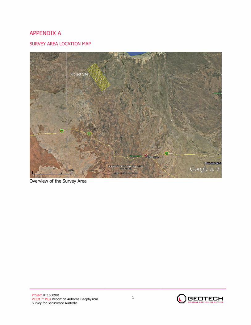
1.2 SURVEY LOCATION The survey area is located at Gregory in Queensland (Figure 2).

Figure 2: Survey area location on Google Earth.

The traverse lines were flown in an east to west (N 145° E azimuth) direction with traverse line spacing of 2000 metres as depicted in Figure 3. Tie lines were neither flown nor planned. For more detailed information on the flight spacing and direction see Table 1.


3

1.3 TOPOGRAPHIC RELIEF AND CULTURAL FEATURES

Topographically, the survey area exhibits a shallow relief with an elevation ranging from 0 to 116 metres above mean sea level over an area of approximately 3215 square kilometres (Figure 3).

There are various ephemeral rivers and streams running through the survey area which connect various lakes. There are visible signs of culture such as roads, power lines and towns are located throughout the survey area.

Figure 3: Flight path over a Google Earth Image.


4

2. DATA ACQUISITION

2.1 FLIGHT LINE SPECIFICATIONS

The survey area (see Figure 3 and Appendix A) and general flight specifications are as follows:

Table 1: Survey Specifications

Survey area boundaries co-ordinates are provided in Appendix B.

2.2 FLYING HEIGHT SPECIFICATIONS During the survey the helicopter was maintained at a mean altitude of 75 metres above the ground with an average survey speed of 100 km/hour. This allowed for an actual average EM Transmitter-receiver loop terrain clearance of 36 metres and a magnetic sensor clearance of 66 metres.

2.3 SURVEY OPERATIONS

Survey operations were based out of Cloncurry, Queensland from November 22nd until December 4th 2016. The following table shows the timing of the flying.

Table 2: Survey schedule

Date Flight

# Flown

km Block Crew location Comments

22-Nov-2016 Cloncurry, Queensland mobilization




26-Nov-2016 1 180 LawnHill Ext Cloncurry, Queensland 180km flown



29-Nov-2016 Cloncurry, Queensland No production due to weather


1-Dec-2016 5 183 LawnHill Ext Cloncurry, Queensland 183km flown

2-Dec-2016 6,7 367 LawnHill Ext Cloncurry, Queensland 367km flown

3-Dec-2016 8,9 371 LawnHill Ext Cloncurry, Queensland 371km flown

4-Dec-2016 10 42 LawnHill Ext Cloncurry, Queensland Remaining kms were flown – flying

complete

1 Note: Actual Line kilometres represent the total line kilometres in the final database. These line-km normally exceed the Planned Line-km, as indicated in the survey NAV files.

Survey block Line spacing (m) Area (Km2)

Planned1 Line-km

Actual

Line-

km

Flight direction Line numbers

Lawn Hill Traverse:2000 3215 1646 1658 N 145° E / N 325° E L5000 – L5170

TOTAL 3215 1646 1658


5

2.4 PROCEDURES The on board operator was responsible for monitoring the system integrity. He also maintained a detailed flight log during the survey, tracking the times of the flight as well as any unusual geophysical or topographic features.

On return of the aircrew to the base camp the survey data was transferred from a compact flash card (PCMCIA) to the data processing computer. The data were then uploaded via ftp to the Geotech office in Aurora for daily quality assurance and quality control by qualified personnel.

2.5 AIRCRAFT AND EQUIPMENT

2.5.1 SURVEY AIRCRAFT The survey was flown using a Eurocopter Aerospatiale (A-star) 350 B3 helicopter, registration VH-VTN. The helicopter is owned and operated by United Aero Helicopters. Installation of the geophysical and ancillary equipment was carried out by a Geotech Ltd crew.

2.5.2 ELECTROMAGNETIC SYSTEM

The electromagnetic system was a Geotech Time Domain EM (VTEM™) with full receiver-waveform streamed data recording at 192 kHz. The “full waveform VTEM system” uses the streamed half-cycle recording of transmitter current and receiver voltage waveforms to obtain a complete system response calibration throughout the entire survey flight. VTEM hardware with the Serial number 12 was used for the survey. The VTEM transmitter current waveform is shown diagrammatically in Figure 4.

The VTEM transmitter loop and Z-component receiver coils were in a concentric-coplanar configuration and their axes are nominally vertical. An X-component receiver coil was also installed in the centre of the transmitter loop, with its axis nominally horizontal and in the flight line direction. The receiver coils measure the dB/dt response, and a B-Field response is calculated during the data processing. The EM transmitter-receiver loop assembly was towed at a mean distance of 38 metres below the aircraft. The configuration is shown in Figure 5.

Figure 4: VTEM™ Transmitter Current Waveform


6

The VTEM™ decay sampling scheme is shown in Table 3 below. Forty-five time measurement gates were used for the final data processing in the range from 0.021 to 10.667 msec. Zero time for the off-time sampling scheme is equal to the current pulse width and is defined as the time near the end of the turn-off ramp where the dI/dt waveform falls to 1/2 of its peak value.

Table 3: Off-Time Decay Sampling Scheme

VTEM™ Decay Sampling Scheme

Index Start End Middle Width

Milliseconds

4 0.018 0.023 0.021 0.005

5 0.023 0.029 0.026 0.005

6 0.029 0.034 0.031 0.005

7 0.034 0.039 0.036 0.005

8 0.039 0.045 0.042 0.006

9 0.045 0.051 0.048 0.007

10 0.051 0.059 0.055 0.008

11 0.059 0.068 0.063 0.009

12 0.068 0.078 0.073 0.010

13 0.078 0.090 0.083 0.012

14 0.090 0.103 0.096 0.013

15 0.103 0.118 0.110 0.015

16 0.118 0.136 0.126 0.018

17 0.136 0.156 0.145 0.020

18 0.156 0.179 0.167 0.023

19 0.179 0.206 0.192 0.027

20 0.206 0.236 0.220 0.030

21 0.236 0.271 0.253 0.035

22 0.271 0.312 0.290 0.040

23 0.312 0.358 0.333 0.046

24 0.358 0.411 0.383 0.053

25 0.411 0.472 0.440 0.061

26 0.472 0.543 0.505 0.070

27 0.543 0.623 0.580 0.081

28 0.623 0.716 0.667 0.093

29 0.716 0.823 0.766 0.107

30 0.823 0.945 0.880 0.122

31 0.945 1.086 1.010 0.141

32 1.086 1.247 1.161 0.161

33 1.247 1.432 1.333 0.185

34 1.432 1.646 1.531 0.214

35 1.646 1.891 1.760 0.245

36 1.891 2.172 2.021 0.281

37 2.172 2.495 2.323 0.323

38 2.495 2.865 2.667 0.370


7

VTEM™ Decay Sampling Scheme

Index Start End Middle Width

Milliseconds

39 2.865 3.292 3.063 0.427

40 3.292 3.781 3.521 0.490

41 3.781 4.341 4.042 0.560

42 4.341 4.987 4.641 0.646

43 4.987 5.729 5.333 0.742

44 5.729 6.581 6.125 0.852

45 6.581 7.560 7.036 0.979

46 7.560 8.685 8.083 1.125

47 8.685 9.977 9.286 1.292

48 9.977 11.458 10.667 1.482

Z Component: 4 - 48 time gates X Component: 20 - 48 time gates


8

VTEM™ system specifications:

Transmitter Receiver

Transmitter loop diameter: 26 m

Number of turns: 4

Effective Transmitter loop area: 2123.7 m2 Transmitter base frequency: 25 Hz

Peak current: 186 A

Pulse width: 7.37 ms

Waveform shape: Bi-polar trapezoid

Peak dipole moment: 395,011 nIA

Average transmitter-receiver loop terrain clearance: 36

metres above the ground

X Coil diameter: 0.32 m

Number of turns: 245

Effective coil area: 19.69 m2 Z-Coil diameter: 1.2 m

Number of turns: 100

Effective coil area: 113.04 m2

Figure 5: VTEM™Plus System Configuration.


9

2.5.3 FULL WAVEFORM VTEM™ SENSOR CALIBRATION

The calibration is performed on the complete VTEM™ system installed in and connected to the helicopter, using special calibration equipment.

The procedure takes half-cycle files acquired and calculates a calibration file consisting of a single stacked half-cycle waveform. The purpose of the stacking is to attenuate natural and man-made magnetic signals, leaving only the response to the calibration signal.

2.5.4 AIRBORNE MAGNETOMETER The magnetic sensor utilized is a Geometrics optically pumped caesium vapour magnetic field sensor mounted 10 metres below the helicopter (when flying), as shown in Figure 5. The sensitivity of the magnetic sensor is 0.02 nanoTesla (nT) at a sampling interval of 0.1 seconds.

2.5.5 GPS NAVIGATION SYSTEM - HELICOPTER The navigation system used was a Geotech PC104 based navigation system utilizing a NovAtel’s WAAS (Wide Area Augmentation System) enabled GPS receiver, Geotech navigate software, a full screen display with controls in front of the pilot to direct the flight and a NovAtel GPS antenna mounted on the helicopter tail (Figure 5). As many as 11 GPS and two WAAS satellites may be monitored at any one time. The positional accuracy or circular error probability (CEP) is 1.8 m, with WAAS active, it is 1.0 m. The co-ordinates of the survey area were set-up prior to the survey and the information was fed into the airborne navigation system. The second GPS antenna is installed on the additional magnetic loop together with Gyro Inclinometer.

2.5.6 GPS LOOP A NovAtel GPS antenna was installed on the front centre of the loop to accurately record the position of the loop (Figure 5). GPS data were sampled every 0.2 seconds. The final GPS coordinates were differentially corrected by post-processing the loop data along with GPS data obtained simultaneously from a base station setup nearby the survey area. Final horizontal coordinates are referenced to GDA94 MGA zone 54 and the height is referenced to the EGM96 geoid. The positional accuracy or circular error probability (CEP) is 1.0 m.

2.5.7 INCLINOMETER LOOP An Anlalog Devices ADIS16405 gyroscopic inclinometer was installed on the loop (Figure 5) to accurately record the orientation of the loop with a sampling interval of 0.1 seconds. The orientation of the loop is determined by three rotation angles based on the local reference frame of the loop: roll (rotation about the x-axis), pitch (rotation about the y-axis) and yaw (rotation about the z-axis). The loop’s reference frame is a right-handed coordinate system with the positive x-axis pointing in the flight direction, positive y-axis pointing to the left of the flight direction and the positive z-axis points vertically upward. Positive rotation for each angle is counter-clockwise about the axis when looking toward the origin (positive roll is left wing up, positive pitch is nose down, positive yaw to the left of the flight direction).


10

2.5.8 RADAR ALTIMETER A Terra TRA 3000/TRI 40 radar altimeter was used to record terrain clearance. The antenna was mounted beneath the bubble of the helicopter cockpit (Figure 5).

2.5.9 LASER ALTIMETER A Schmitt Industries AR3000 laser altimeter was used which has an altitude range 0.5 to 300m and accuracy ±5cm. The laser altimeter was located at the front of the horizontal magnetic gradient loop with a GPS antenna and inclinometer and the data was sampled at an interval of 0.2 seconds.

2.5.10 DIGITAL ACQUISITION SYSTEM

A Geotech data acquisition system recorded the digital survey data on an internal compact flash card. Data is displayed on an LCD screen as traces to allow the operator to monitor the integrity of the system. The data type and sampling interval as provided in Table 4 Table 4: Acquisition Sampling Rates

Data Type Sampling

TDEM 0.1 sec

Magnetometer 0.1 sec

GPS Position 0.2 sec

Radar Altimeter 0.2 sec

Laser Altimeter 0.2 sec

Gyro Inclinometer 0.1 sec

2.6 BASE STATION A combined magnetometer/GPS base station was utilized on this project. A Geometrics Caesium vapour magnetometer was used as a magnetic sensor with a sensitivity of 0.001 nT. The base station was recording the magnetic field together with the GPS time at 1 Hz on a base station computer.

The base station magnetometer sensors were installed at Gregory airport (18º38.1678’S, 139º14.0207’E) away from electric transmission lines and moving ferrous objects such as motor vehicles. The base station data were backed-up to the data processing computer at the end of each survey day.


11

2.7 TEST LINES AND CALIBRATION PROCEDURES

2.7.1 FULL WAVEFORM VTEM CALIBRATION The calibration is performed with the completely assembled VTEM system connected to the helicopter at the survey site on the ground. Measurements of the half-cycles are collected and used to calculate a sensor calibration consisting of a single stacked half-cycle waveform. The purpose of the stacking is to attenuate natural and man-made magnetic signals, leaving only the response to the calibration signal. The stacked half-cycle allows the transfer functions between the receiver and data acquisition system, HD (ω), and current sensor and data acquisition system, HR (ω), to be determined. These transfer functions are used as a part of the system response correction during processing to correct the half-cycle waveforms and data acquired on a survey flight to a common transfer function: D(ω)=[(H_C (ω))⁄(H_D (ω) )] D_R (ω) A(ω)=[(H_C (ω))⁄(H_R (ω) )] A_R (ω) Where HC(ω) is the common transfer function, and DR(ω) and AR(ω) are the FFT’s of the raw receiver and current sensor responses recorded by the data acquisition system. This process allows for the receiver response, R(ω), to become independent of the sensor characteristics determined by the transfer functions HD(ω) and HR(ω) and acts similar to a deconvolution of the data. R(ω)=D(ω)I(ω)/A(ω) Where, D(ω) is the FFT of the actual receiver data sample D(t), I(ω) is the FFT of a reference or “Ideal waveform” and A(ω) is the FFT of the actual waveform.

2.7.2 HIGH ALTITUDE CALIBRATION High altitude calibrations were conducted at the beginning, during, and end of each flight. The calibration’s objective is to determine the EM “zero level” by climbing to an altitude of 1,000 metres above ground to measure the receiver’s response absent of response due to the ground. When at the required altitude, at least 60 seconds of data were acquired in normal operation mode. The final delivered dataset contains these processed windowed high altitude data for the ten (10) survey flights in ASCII column format (Table 5) Reference transmitter current and receiver voltage waveforms, each sampled at 192 kHz, were also recorded at high altitude for all survey flights. The recorded waveforms were transformed into an ideal form, having zero current at the beginning of the off-time, by the Full Waveform calibration (see Section 2.7.1). A graphical representation of a VTEM waveform is shown in Figure 4.


12

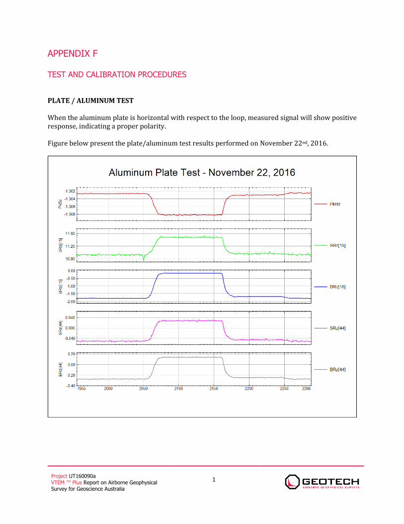
2.7.3 PLATE TEST This test is performed on ground to verify the sensitivity of the system. An aluminium plate of known conductive response is positioned in alternated positions (vertical and horizontal) for about 10 seconds for three time measurements. Response of corresponding dB/dt and B-field data is then verified. The Plate test was performed at the beginning of the survey on November 22nd, 2016. Result of this test is presented in a Geosoft database view in Appendix F.

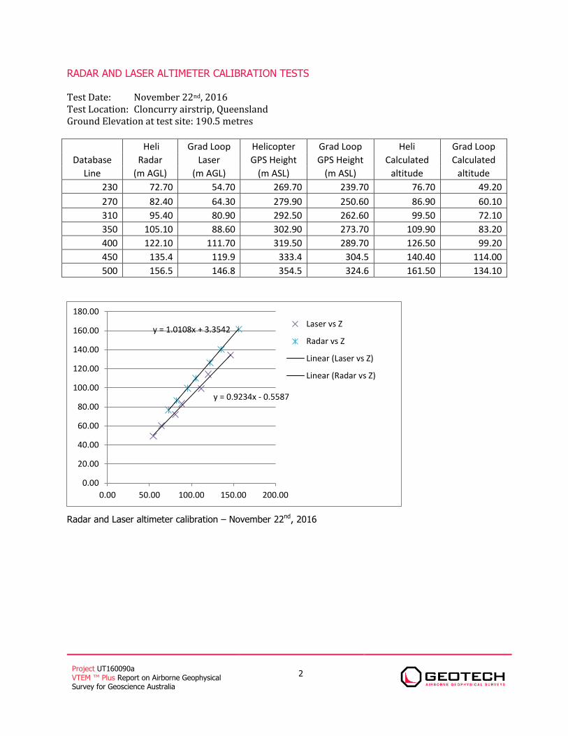
2.7.4 RADAR AND LASER ALTIMETERS The purpose of radar and laser altimeter calibration is to verify the performance of the altimeter readings using the GPS height data as the reference. The calibration was performed by flying over the same spot at various altitudes, ranging from 70m (230 ft) to 152m (500 ft) according to the radar altimeter which is positioned on the helicopter front. The selected spot in the Cloncurry Airstrip, Queensland (Figure 6) have known elevation and flat terrain. This test was performed on November 22nd, 2016.

Figure 6: Location of the radar and laser altimeter test site on Google EarthTM image; Cloncurry airstrip

The calibration results are presented in Appendix F. The graphs of the GPS heights plotted against the radar and laser altimeter readings demonstrate that there is a linear relationship between all GPS and altimeter instruments (R2 = 0.99), for the range of flying heights tested.


13

3. PERSONNEL The following Geotech Ltd. personnel were involved in the project.

FIELD: Project Manager: Leon Lovelock (Office) Data QC: Neil Fiset (Office) Crew chief: Peter Macdonald Operator: Chris Botman The survey pilot and the mechanical engineer were employed directly by the helicopter operator – United Aero Helicopters. Pilot: Colby Tyrell Clayton Lucht Mechanical Engineer: n/a OFFICE: Preliminary Data Processing: Neil Fiset Final Data Processing: Timothy Eadie Keeme Mokubung Karl Kwan Final Data QA/QC: Geoffrey Plastow Reporting/Mapping: Wendy Acorn Processing and Interpretation phases were carried out under the supervision of Geoffrey Plastow, P. Geo, and Data Processing Manager. The customer relations were looked after by Rod Fowler.


14

4. DATA PROCESSING AND PRESENTATION Data compilation and processing were carried out by the application of Geosoft OASIS Montaj and programs proprietary to Geotech Ltd.

4.1 FLIGHT PATH, COORDINATES AND PARALLAX CORRECTION The flight path data, recorded by the acquisition program as WGS 84 latitude/longitude, were differentially corrected using the base station GPS and converted into the GDA94 Datum, Map Grid of Australia Zone 54 coordinate system in Oasis Montaj. Both sets of GPS coordinate, from helicopter GPS and gradiometer GPS, were linearly interpolated between each measurement sampled every 0.2 seconds to match the sampling rate of the TDEM and magnetic datasets at every 0.1 seconds. The coordinates labelled “GradLoop_*” in Table 5 & Table 6 refer to the position of the gradiometer GPS antenna located at the front of the gradiometer loop. A further set of coordinates, labelled “EM_Mag_Data_*” were then calculated for the position halfway between the center of the gradiometer loop. This position represents the centre of the gradiomter loop and is the point where the tow cable intersects the plane of the gradiometer loop. This was achieved by projecting backwards along the flight line by 6.25 m, the radius of the gradiometer loop, from the gradiometer loop GPS antenna position. A parallax correction was applied to the EM data to account for the distance by which the EM transmitter-receiver loop lags behind the centre of the gradiometer loop. In this parallax correction the EM data are shifted toward lower fiducial numbers by the nearest integer number of fiducials that it would take to travel the average horizontal distance Δx2 (see Figure 7 and formulae below) which separates the centres of the gradiometer and EM loops based on the average helicopter speed for each line. The magnetic data are shifted in the same manner backward towards the centre of the gradiometer loop. Thus the “EM_Mag_Data_*” coordinates are the set of coordinates that the EM and magnetic data are parallax corrected for, and to which all EM and magnetic data and interpretations should be referred.

4.2 CALCULATION OF HEIGHT OF THE EM TRANSMITTER RECEIVER LOOP AND MAGNETIC SENSOR

The EM transmitter-receiver loop height above ground was calculated from data from the radar altimeter located on the helicopter, and data from the laser altimeter and gyroscopic inclinometer located on the front of the magnetic gradiometer loop, and knowledge of the tow cable lengths.


15

The procedure requires calculation of the unknown vertical distance between the magnetic gradiometer loop and EM transmitter-receiver loop. This process is summarized in the formula below, where; laser is the laser altimeter measurement, radar is the radar altimeter measurement, l1 is the length along the tow cable from the helicopter to the center of the gradiometer loop equal to 30.4 meters, l2 is the length along the tow cable from the center of the gradiometer loop to the center of the transmitter-receiver loop equal to 11.1 meters, and δz is the vertical deflection of the front of the gradiometer loop from the center which can be calculated from the pitch angle and magnetic gradiometer loop radius of 6.25m. These variables are illustrated in Figure 7 showing the VTEM system with an exaggerated pitch. For the magnetic sensor, l3 is the distance from the base of the helicopter along the tow cable to the magnetic sensor, equals to 13.4 meters. The horizontal distance between the radar and the GPS antenna mounted in the helicopter equals 10.45 meters.

TxRx Height = laser + δz − l2 (radar − laser − δz

l1)

∆x2 = √(l2)2 − (Δz2)2, where,

Δz2 = l2 (radar − laser − δz

l1).

Figure 7: Calculation of EM transmitter loop height

11.1m

13.4m

30.4m


16

4.3 DIGITAL ELEVATION MODEL Two digital elevation models (DEMs) were calculated. They were calculated from the helicopter GPS and radar altimeter, and also from the magnetic gradiometer loop GPS and laser altimeter. The formulas used to calculate the DEMs are shown below.

DEMradar = (ZGPS Heli + NEGM96 − NAUSGEOID09) − radar − 2.5

DEMlaser = (ZGPS GradLoop + NEGM96 − NAUSGEOID09) − laser

The term NEGM96 - NAUSGEOID09, accounts for the difference between the EGM96 geoid, which the GPS heights are referenced to, and the AUSGEOID09, which both DEMs are referenced to. The 2.5 metre offset, for the radar altimeter derived DEM, accounts for the vertical separation between the helicopter GPS antenna located on the tail and the radar altimeter located below the noise of the helicopter.

4.4 ELECTROMAGNETIC DATA As the data are acquired by the data acquisition system on the helicopter, it goes through a digital filter to reject major sferic events and is stacked to further reduce system noise. Afterward, the streamed data is processed by applying a system response correction, B-field integration, time window binning, compensation, filtering, and leveling. Four stages of processing of the EM data have been delivered. They are denoted in the final point-located EM dataset (Table 5) as;

1. Raw (Raw), 2. Compensated (Comp), 3. Filtered (Flt), 4. Final (F).

The digital filtering process is a three stage filter used to reject major sferic events and reduce system noise. Local sferic activity can produce sharp, large amplitude events that cannot be removed by conventional filtering procedures. Smoothing or stacking will reduce their amplitude but leave a broader residual response that can be confused with geological phenomena. To avoid this possibility, a computer algorithm searches out and rejects the major sferic events. The data was then stacked using 15 half cycles, 0.3 seconds, to create a stacked half-cycle waveform at 0.1 second intervals. The stacking coefficients are tapered with a shape that approximates a Gaussian function. During post-flight processing, the streamed data have a sensor response correction applied which corrects the receiver channels and current monitor to a common impulse response based on the Full Waveform calibration (see Section 2.7.1). The B-field data are calculated by integrating the dB/dt cycles from the 192 kHz streamed data. Then, the streamed data are converted into a set of time window channels (see Table 3) to reduce noise levels further. The output of this stage is the data denoted as “Raw” in Table 5.


17

The data have noise levels reduced further by the use of an EM compensation procedure which removes characteristic noise from each fiducial determined by the difference between the transmitter and bucking loop fields at the receiver during the flight. This is achieved by a statistical correlation between each time window channel and primary field measurement taken during the on-time. The data channels which have been processed to this point are denoted by “Compensated” in Table 5 Next, filtering of the electromagnetic data was performed in two steps. The first is a 4 fiducial wide non-linear filter to eliminate any large spikes remaining in the dataset. The second filter is a low pass symmetric linear digital filter that has zero phase shift which prevents any lag or peak displacement from occurring, and it suppresses only variations with a wavelength less than about 1 second or 25

metres. The output of this stage is the data channels denoted as “Filtered” in Table 5 To remove the remaining system response from the data, a “zero level” estimate was subtracted from the data at each fiducial. First, the “zero level” correction was applied which was calculated by linear interpolation of the high altitude backgrounds (see Section 2.7.2) recorded two or more times during each survey flight. Second, a statistical leveling correction was applied to the EM data which utilizes the high altitude data recorded for each flight and the survey line data to compute the

additional leveling correction. This produces the EM data denoted as “Final” in Table 5

VTEM™ has two receiver coil orientations. Z-axis coil is oriented parallel to the transmitter coil axis and both are horizontal to the ground. The X-axis coil is oriented parallel to the ground and along the line-of-flight. This combined two coil configuration provides information on the position, depth, dip and thickness of a conductor. Generalized modeling results of VTEM data, are shown in Appendix D.

In general X-component data produce cross-over type anomalies: from “+ to – “in flight direction of flight for “thin” sub vertical targets and from “- to +” in direction of flight for “thick” targets. Z component data produce double peak type anomalies for “thin” sub vertical targets and single peak for “thick” targets.

The limits and change-over of “thin-thick” depends on dimensions of a TEM system (Appendix D, Figure D-16).

4.5 CONDUCTIVITY DEPTH IMAGING A set of Conductivity Depth Images (CDI) were generated using EM Flow version 3.3, developed by Encom Technologies Pty Ltd. A total of forty-five (45) dB/dt Z component channels, starting from channel 4 (21 µsec) to channel 48 (10667 µsec), were used for the CDI calculation. An averaged waveform at the receiver was used for the calculation since it was consistent for the majority of the flights with minor deviation from the average. The waveform used is consistent with those supplied and outlined in Table 6. The main steps to calculate the CDI in EM Flow are described in the following points: 1. System definition (units, waveform shape and half period, system geometry and input data

format) 2. Conversion from ASCII file format to Binary file format (smoothing option disabled) 3. Basis Function creation. Number of Taus equalled 44 (approximately equal to the number of

channels). Tau range was 0.02 ms to 7.5 ms. Number of Eigenvectors was 12. 4. Deconvolution: PLS algorithm. Smoothing set to 0.2 and minimum length to 0.1.


18

Normalization by absolute maximum. Error tolerance at 1.0e-04. No error weighting. 5. CDI Matrix Calculation: Tau range at all (1-44). Maximum altitude at 500 metres and

maximum depth at 400 metres. Depth resolution of 1 metre. Depth of investigation cut-off factor equal to 1. Both exponential and layered models were generated.

6. Data export: Geosoft Line Database.

The final delivered CDI dataset (Table 6) contains estimated conductivities as an array with 70 elements with a depth resolution of 5 metres, for depths from 5 metres to 350 metres.

Conductivity Depth Slices were calculated from the 1 metre depth resolution data output from EM Flow by averaging conductivity values within the specified depth ranges, inclusively.

4.6 MAGNETIC DATA

The processing of the magnetic data involved the correction for diurnal variations by using the digitally recorded ground base station magnetic values. The base station magnetometer data was edited and merged into the Geosoft GDB database on a daily basis. The aeromagnetic data was corrected for diurnal variations by subtracting the observed magnetic base station deviations. The removal of the International Geomagnetic Reference Field is then applied based on the IGRF model provided for each flight date over the survey lines. A magnetic field of 49,136 nT is added back to the data.


19

5. DELIVERABLES

5.1 SURVEY REPORT The survey report describes the data acquisition, processing, and final presentation of the survey results. The survey report is provided in two paper copies and digitally in PDF format.

5.2 DIGITAL DATA Point located data files in ASCII column format, with accompanying README header files that describe the data file content, were supplied for the processed EM and ancillary data. This included files for the regular survey lines, traverses, repeat lines and high altitude lines. The delivered data channels listed in Table 5 refer to Table 3 for the time definitions for channels 4 to 48.

Table 5: Contents of the ASCII columns datasets for the point located EM data

Channel name Units Description

GAproject Geoscience Australia Project Number

GTproject Geotech Ltd Project Number

FltNo Flight Number

LineNo Line Number

Fiducial Fiducial Number

Date Date

Time Seconds Seconds since midnight local time

Bearing Degrees Flight Direction Azimuth

Heli_Lon Degrees Helicopter GPS Longitude (GDA94)

Heli_Lat Degrees Helicopter GPS Latitude (GDA94)

Heli_Easting metres Helicopter GPS Easting (GDA94, MGA54†)

Heli_Northing metres Helicopter GPS Northing (GDA94, MGA54)

Heli_Height metres Helicopter GPS height above EGM96 Geoid

Heli_GPSTime seconds Helicopter GPS second of the GPS week

Radar_raw metres Raw helicopter radar altimeter height above ground

Radar metres Helicopter radar altimeter height above ground

GradLoop_Lon degrees Gradiometer Loop GPS Longitude (GDA94)

GradLoop_Lat degrees Gradiometer Loop GPS Latitude (GDA94)

GradLoop_Easting metres Gradiometer Loop GPS Easting (GDA94, MGA54)

GradLoop_Northing metres Gradiometer Loop GPS Northing (GDA94, MGA54)

GradLoop_Height metres Gradiometer Loop GPS height above EGM96 Geoid

GradLoop_GPSTime seconds Gradiometer Loop GPS second of the GPS week

Laser_raw metres Raw gradiometer Loop laser altimeter height above

ground

Laser metres Gradiometer Loop laser altimeter height above ground

Roll degrees Gradiometer Loop rotation about the in-line (x) axis

Pitch degrees Gradiometer Loop rotation about the cross-line (y) axis

Yaw degrees Gradiometer Loop rotation about the vertical (z) axis

EM_Mag_Data_Lon degrees Derived longitude of centre of magnetic gradiometer loop – reference point for EM and Mag data (GDA94)

EM_Mag_Data_Lat degrees Derived latitude of centre of magnetic gradiometer loop

– reference point for EM and Mag data (GDA94)

EM_Mag_Data_Easting metres Derived easting of centre of magnetic gradiometer loop

– reference point for EM and Mag data (GDA94,


20


MGA54)

EM_Mag_Data_Northing metres Derived northing of centre of magnetic gradiometer loop – reference point for EM and Mag data (GDA94,

MGA54)

EM_Loop_Height metres Derived height of centre of the EM Loop above ground

DEM_laser_final metres Digital Elevation Model (Australian Height Datum)

derived from laser altimeter and Gradiometer Loop GPS

DEM_radar_final metres Digital Elevation Model (Australian Height Datum) derived from radar altimeter and Helicopter GPS

MagRaw nT Measured Total Magnetic field

Mag_Level nT Diurnal and IGRF corrected Total Magnetic field

Basemag nT Base station mag

IGRF_Tot nT IGRF Total Field

Mag_Height m Derived height of magnetic sensor above ground

TransCurr Amps Transmitter Current

PLM 50 Hz power line monitor

SRawz[4-48] pV/(A*m4) Raw Z dB/dt data channels 4 to 48

SCompz[4-48] pV/(A*m4) Compensated Z dB/dt data channels 4 to 48

SFltz[4-48] pV/(A*m4) Filtered Z dB/dt data channels 4 to 48

SFz[4-48] pV/(A*m4) Final Z dB/dt data channels 4 to 48

BRawz[4-48] (pV*ms)/(A*m4) Raw Z B-Field data channels 4 to 48

BCompz[4-48] (pV*ms)/(A*m4) Compensated Z B-Field data channels 4 to 48

BFltz[4-48] (pV*ms)/(A*m4) Filtered Z B-Field data channels 4 to 48

BFz[4-48] (pV*ms)/(A*m4) Final Z B-Field data channels 4 to 48

SRawx[20-48] pV/(A*m4) Raw X dB/dt data channels 20 to 48

SCompx[20-48] pV/(A*m4) Compensated X dB/dt data channels 20 to 48

SFltx[20-48] pV/(A*m4) Filtered X dB/dt data channels 20 to 48

SFx[20-48] pV/(A*m4) Final X dB/dt data channels 20 to 48

BRawx[20-48] (pV*ms)/(A*m4) Raw X B-Field data channels 20 to 48

BCompx[20-48] (pV*ms)/(A*m4) Compensated X B-Field data channels 20 to 48

BFltx[20-48] (pV*ms)/(A*m4) Filtered X B-Field data channels 20 to 48

BFx[20-48] (pV*ms)/(A*m4) Final X B-Field data channels 20 to 48

†MGA54 = Map Grid of Australia Zone 54

Point located data files were supplied in ASCII column format, with accompanying README header files, for the processed conductivity depth imaging results and ancillary data. This included files for the regular survey lines, traverses, and repeat lines. The delivered data channels are listed in Table 6.

Table 6: Contents of the ASCII columns dataset for the point located CDI data


GAproject Geoscience Australia Project Number

GTproject Geotech Ltd Project Number

FltNo Flight Number

LineNo Line Number

Fiducial Fiducial Number

Date Date

Time Seconds Seconds since midnight local time

Bearing Degrees Flight Direction Azimuth

Heli_Lon Degrees Helicopter GPS Longitude (GDA94)

Heli_Lat Degrees Helicopter GPS Latitude (GDA94)


21


Heli_Easting metres Helicopter GPS Easting (GDA94, MGA54)

Heli_Northing metres Helicopter GPS Northing (GDA94, MGA54)

Heli_Height metres Helicopter GPS height above EGM96 Geoid

Heli_GPSTime seconds Helicopter GPS second of the GPS week

Radar metres Helicopter radar altimeter height above ground

GradLoop_Lon degrees Gradiometer Loop GPS Longitude (GDA94)

GradLoop_Lat degrees Gradiometer Loop GPS Latitude (GDA94)

GradLoop_Easting metres Gradiometer Loop GPS Easting (GDA94, MGA54)

GradLoop_Northing metres Gradiometer Loop GPS Northing (GDA94, MGA54)

GradLoop_Height metres Gradiometer Loop GPS height above EGM96 Geoid

GradLoop_GPSTime seconds Gradiometer Loop GPS second of the GPS week

Laser metres Gradiometer Loop laser altimeter height above

ground

Roll degrees Gradiometer Loop rotation about the in-line (x) axis

Pitch degrees Gradiometer Loop rotation about the cross-line (y)

axis

Yaw degrees Gradiometer Loop rotation about the vertical (z) axis

EM_Mag_Data_Lon degrees Derived longitude of centre of magnetic gradiometer

loop – reference point for EM and Mag data (GDA94)

EM_Mag_Data_Lat degrees Derived latitude of centre of magnetic gradiometer loop – reference point for EM and Mag data (GDA94)

EM_Mag_Data_Easting metres Derived easting of centre of magnetic gradiometer

loop – reference point for EM and Mag data (GDA94, MGA54)

EM_Mag_Data_Northing metres Derived northing of centre of magnetic gradiometer

loop – reference point for EM and Mag data (GDA94, MGA54)

EM_Loop_Height metres Derived height of centre of the EM Loop above ground

DEM_laser_final metres Digital Elevation Model (Australian Height Datum)

derived from laser altimeter and Gradiometer Loop GPS

DEM_radar_final metres Digital Elevation Model (Australian Height Datum)

derived from radar altimeter and Helicopter GPS

MagRaw nT Measured Total Magnetic field

Mag_Level nT Diurnal and IGRF corrected Total Magnetic field

Basemag nT Base station mag

IGRF_Tot nT IGRF Total Field

Mag_Height m Derived height of magnetic sensor above ground

TransCurr Amps Transmitter Current

PLM 50 Hz power line monitor

Cond_5m [0-70] S/m Conductivity Depth Imaging from 5 to 350 metres depth for every 5 metres

Cond_Depth_Slice_0_5m S/m Conductivity Depth Slice between 0 and 5 metres

depth


depth

Cond_Depth_Slice_10_15m S/m Conductivity Depth Slice between 10 and 15 metres depth


depth


22



depth


depth



depth

Cond_Depth_Slice_100_150m S/m Conductivity Depth Slice between 100 and 150

metres depth


Cond_Depth_Slice_200_300m S/m Conductivity Depth Slice between 200 and 300

metres depth

Data files were supplied in ASCII column format, with accompanying README header files, for the 192 kHz sampling of the waveform acquired at high altitude for every flight. The delivered waveform data are listed in Table 7.

Table 7: Contents of the ASCII columns datasets for the waveform data


Flight Flight number

Time milliseconds Time of current sample

Tx_Current Amps Transmitter Current

Rx_voltage Volts Receiver voltage

Gridded data were supplied in ER Mapper (.ers) format at 500 metre cell size.

Table 8: List of gridded data included in the final dataset

Grid name Description

DEM_radar_final Radar altimeter derived digital elevation model

Mag2 Total magnetic intensity

CDI_Depth_Slice_0_5 Conductivity Depth Slice between 0 and 5 metres depth












23

Respectfully submitted2,

___________________________ ___________________________

Neil Fiset Timothy Eadie Geotech Ltd Geotech Ltd ___________________________ ___________________________ Karl Kwan Keeme Mokubung Geotech Ltd Geotech Ltd ____________________________________________ Geoffrey Plastow, P. Geo. Data Processing Manager Geotech Ltd March, 2017

2 Final data processing of the EM and magnetic data were carried out by Neil Fiset, Timothy Eadie, Keeme Mokubung, and Karl Kwan

from the office of Geotech Ltd. in Aurora, Ontario, under the supervision of Geoffrey Plastow, P.Geo. Data Processing Manager.


1

APPENDIX A

SURVEY AREA LOCATION MAP

Overview of the Survey Area


1

APPENDIX B SURVEY AREA COORDINATES (GDA94, MGA Zone 54 South)

X Y

278707 8017829

249935 7997956

302877 7921612

330457 7944186


1

APPENDIX C

FLIGHT LINE SUMMARY

Line : Flight number Start Fiducial End Fiducial

L5000:1 18061 49375

L5010:1 62391 97745

L5020:2 17098 46648

L5030:2 63115 84566

L5031:10 15719 29885

L5040:3 19543 53768

L5050:3 66517 97967

L5060:4 17534 49598

L5070:4 63568 96745

L5080:5 18550 55869

L5090:5 67419 96837

L5100:6 18299 54481

L5110:6 65871 96745

L5120:7 17251 58268

L5130:7 71603 105103

L5140:8 17703 49725

L5150:8 65196 99794

L5160:9 23432 59907

L5170:9 72916 106022


1

APPENDIX D GENERALIZED MODELING RESULTS OF THE VTEM SYSTEM INTRODUCTION The VTEM system is based on a concentric or central loop design, whereby, the receiver is positioned at the centre of a transmitter loop that produces a primary field. The wave form is a bi-polar, modified square wave with a turn-on and turn-off at each end.

During turn-on and turn-off, a time varying field is produced (dB/dt) and an electro-motive force (emf) is created as a finite impulse response. A current ring around the transmitter loop moves outward and downward as time progresses. When conductive rocks and mineralization are

encountered, a secondary field is created by mutual induction and measured by the receiver at the centre of the transmitter loop.

Efficient modeling of the results can be carried out on regularly shaped geometries, thus yielding close approximations to the parameters of the measured targets. The following is a description of a series of common models made for the purpose of promoting a general understanding of the measured results.

A set of models has been produced for the Geotech VTEM™ system dB/dT Z and X components (see models D1 to D15). The Maxwell TM modeling program (EMIT Technology Pty. Ltd. Midland, WA, AU) used to generate the following responses assumes a resistive half-space. The reader is encouraged to review these models, so as to get a general understanding of the responses as they apply to survey results. While these models do not begin to cover all possibilities, they give a general perspective on the simple and most commonly encountered anomalies. As the plate dips and departs from the vertical position, the peaks become asymmetrical.

As the dip increases, the aspect ratio (Min/Max) decreases and this aspect ratio can be used as an

empirical guide to dip angles from near 90º to about 30º. The method is not sensitive enough where dips are less than about 30º.


2

Figure D-1: vertical thin plate Figure D-2: inclined thin plate

Figure D-3: inclined thin plate Figure D-4: horizontal thin plate

Figure D-5: horizontal thick plate (linear scale of the

response)

Figure D-6: horizontal thick plate (log scale of

the response)


3

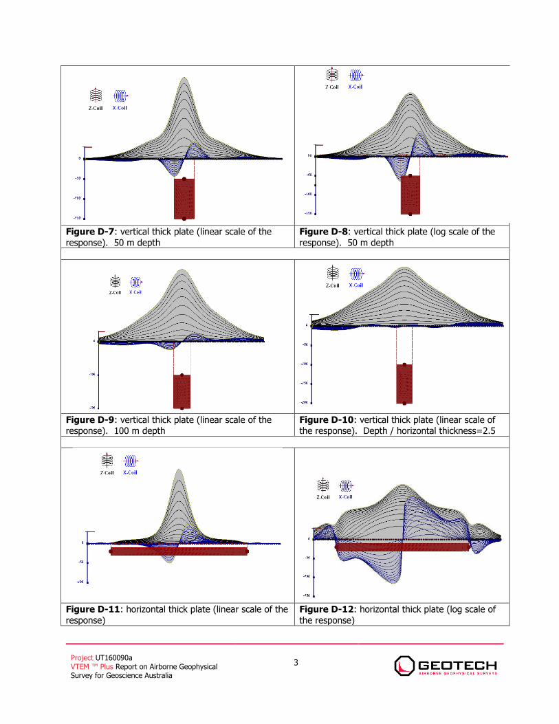
Figure D-7: vertical thick plate (linear scale of the

response). 50 m depth

Figure D-8: vertical thick plate (log scale of the

response). 50 m depth

Figure D-9: vertical thick plate (linear scale of the response). 100 m depth

Figure D-10: vertical thick plate (linear scale of the response). Depth / horizontal thickness=2.5

Figure D-11: horizontal thick plate (linear scale of the

response)

Figure D-12: horizontal thick plate (log scale of

the response)


4

Figure D-13: inclined long thick plate Figure D-14: two vertical thin plates

Figure D-15: two horizontal thin plates Figure D-16: two vertical thick plates


5

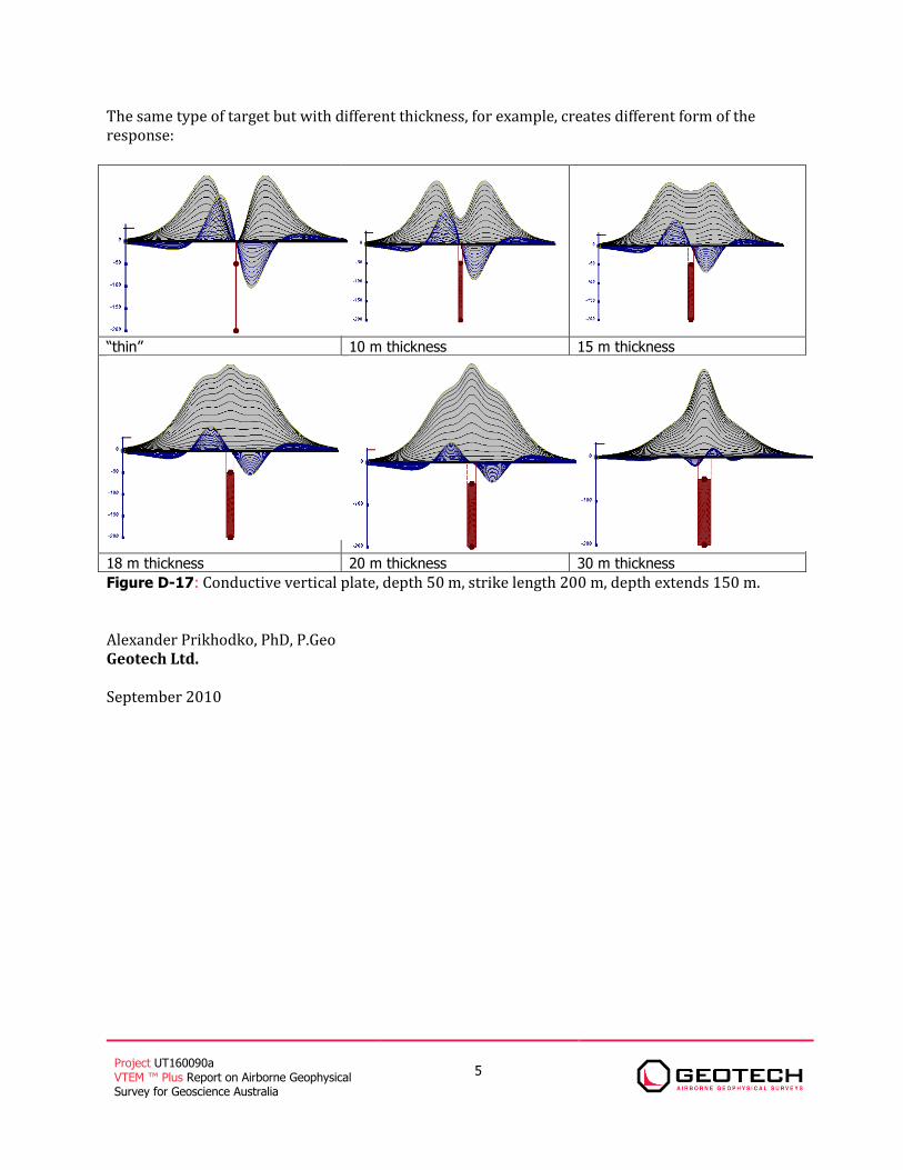
The same type of target but with different thickness, for example, creates different form of the response:

“thin” 10 m thickness 15 m thickness

18 m thickness 20 m thickness 30 m thickness

Figure D-17: Conductive vertical plate, depth 50 m, strike length 200 m, depth extends 150 m. Alexander Prikhodko, PhD, P.Geo Geotech Ltd. September 2010


1

APPENDIX E

CONDUCTIVITY DEPTH IMAGES MULTI PLOTS Multi-parameter plots are presented for each survey line. These plots include, from top to bottom, (1) pitch and roll of the transmitter-receiver, (2) transmitter-receiver height, (3) power line monitor, 4) magnetics TMI and first vertical derivative, (5) dBz/dt profiles, (6) conductivity-depth image (CDI) in logarithmic colour scale, and (7) CDI in linear colour scale.


1

APPENDIX F TEST AND CALIBRATION PROCEDURES PLATE / ALUMINUM TEST When the aluminum plate is horizontal with respect to the loop, measured signal will show positive response, indicating a proper polarity. Figure below present the plate/aluminum test results performed on November 22nd, 2016.


2

RADAR AND LASER ALTIMETER CALIBRATION TESTS

Test Date: November 22nd, 2016 Test Location: Cloncurry airstrip, Queensland Ground Elevation at test site: 190.5 metres

Heli Grad Loop Helicopter Grad Loop Heli Grad Loop

Database Radar Laser GPS Height GPS Height Calculated Calculated

Line (m AGL) (m AGL) (m ASL) (m ASL) altitude altitude

230 72.70 54.70 269.70 239.70 76.70 49.20

270 82.40 64.30 279.90 250.60 86.90 60.10

310 95.40 80.90 292.50 262.60 99.50 72.10

350 105.10 88.60 302.90 273.70 109.90 83.20

400 122.10 111.70 319.50 289.70 126.50 99.20

450 135.4 119.9 333.4 304.5 140.40 114.00

500 156.5 146.8 354.5 324.6 161.50 134.10

Radar and Laser altimeter calibration – November 22nd, 2016

y = 0.9234x - 0.5587

y = 1.0108x + 3.3542

0.00

20.00

40.00

60.00

80.00

100.00

120.00

140.00

160.00

180.00

0.00 50.00 100.00 150.00 200.00

Laser vs Z

Radar vs Z

Linear (Laser vs Z)

Linear (Radar vs Z)

report on a combined helicopter borne ut160090a vtem plus report on airborne geophysical survey for...

Documents