repeated- measures 8 designs · designs, statistics, interpretation, and write-up in apa style. 8....

107

8

8Repeated-Measures

Designs

Everybody Plays!

In Chapter 7, you learned about research designs that rely on observing dif-ferent groups of participants. There is another group of research designs that

allows you to test the same people more than once; these are called repeated-measures designs. When you use these designs, each person experiences every level of the independent variable (IV). For example, you might want to measure how fast your participants can type when they are working in the presence of other people or alone, a social facilitation effect. You have a choice about how to manipulate this variable. You could randomly assign half of your participants to each of two groups (a between-groups design described in the previous chapter). Or you could ask all of your participants to type the same passage as fast as they can under each of the two conditions, which would be a repeated-measures design.

There are a number of reasons why you might choose to use a repeated-measures design. The major advantage of testing the same people twice is that you prevent the range of individual differences from affecting your outcome. In this case, the baseline speed of typing for each person will be the same in both experimental conditions. Furthermore, it is not possible to accidently assign all of the fast typists to one condition or the other because they are represented in both conditions. So, using repeated-measures prevents an accidental confound between social condition and natural typing speed. Another way to think about this is that with a repeated-measures design, you start off equalizing typing speed in the two conditions. Now it should be easier to see if you can alter that

Copyright ©2019 by SAGE Publications, Inc. This work may not be reproduced or distributed in any form or by any means without express written permission of the publisher.

Do not

copy

, pos

t, or d

istrib

ute

108 D E S I G N S , S TAT I S T I C S , I N T E R P R E TAT I O N , A N D W R I T E - U P I N A PA S T Y L E

8

speed by manipulating the social condition within the same person. When indi-viduals serve as their own controls in this way, we are guaranteed to start with the same distribution of individual differences in each condition, that is, the same range of typing speeds as well as the same number of slow and fast typists.

As you might imagine, comparing a person’s performance in one condition to the same person’s performance in another situation is more powerful than mak-ing comparisons across different groups of participants. Remember that statisti-cal power is the probability of rejecting the null hypothesis when the research hypothesis is true. We want statistical power to be high. A repeated-measures research design makes it more likely that you will support your research hypo th-esis if it is true. As a result, a small difference in typing time between the two con-ditions based on being watched or not is more likely to be statistically significant.

This design is so powerful that you might wonder why we would use any other type of design. Unfortunately, some drawbacks do exist. You probably learned about carryover effects in your research methods course. In our typ-ing example, we might expect that practice with typing in the first condition will speed up typing in the second. If all of your participants typed alone first and then typed with others second, the practice effect would be confounded with social condition. If you find a difference in the two conditions, you would not know if it was caused by the order of the conditions (i.e., typing alone followed by typing with others) or the social conditions. However, we can control for practice effects by counterbalancing the IV conditions; half of the participants type alone first and then with others, and the other half type with others first and then alone. To make sure that order does not influence our results, we can simply include order as an additional IV when we analyze our data. The design for this analysis is presented in Chapter 9.

Of course, sometimes you cannot counterbalance the IV conditions. For example, imagine that we want to test the effectiveness of a “new miracle cure” for Parkinson’s disease. We cannot give half of our participants the “new miracle cure” first and then give those same patients a placebo, particularly if the cure worked! Even if the cure was reversible, it would not be ethical to withdraw the drug and return our participants to their debilitated state. In such a situation, we can still use a repeated-measures design and measure symptoms pre-“cure” and post. While not ideal, there are times when we might not have an alternative to this quasi-experimental design.

Repeated-measures designs offer the same range of designs as between-groups designs, including two or more IVs (or pseudo-IVs) and two or more levels of each independent variable. Just as we did in Chapter 8, we will go through examples starting with the simplest and moving on to a useful and complex design.

One Independent Variable With Two Levels

The simplest repeated-measures design is represented by the “typing” example we presented above. In this design, you would have one IV (how many people


Do not

copy

, pos

t, or d

istrib

ute

Repeated-Measures Designs 109

8

were present while our participants were typing) with two levels (either some people or none). Of course, you need to arrange for all participants to experi-ence both levels of the IV. In this case, we ask all of our participants to type two similar documents, one alone and a second in the company of five other people. To control for carryover effects, we could randomly assign participants to type either alone or in the company of others first. So half of the participants would type alone first and the other half would type in the company of others first. You would use a paired-samples t-test to analyze your data for a mean difference in typing time (your DV) between the two conditions. Notice that in this analysis, we do not bother with testing the order of conditions as a second IV. We just accept that any additional variability from order of testing will equally affect both groups because we counterbalanced order. However, we want you to know that we could use the mixed design described in Chapter 9 to make sure that order of the social conditions did not affect typing time.

Let us take a look at what might happen if we actually conducted the social facilitation experiment that is described above. We will bring a group of partici-pants into the lab. Half of them would type the passage while alone first and then a second time while in the presence of others; the other half of our participants would experience the experimental conditions in the opposite order. This design has one IV with two levels (social and alone) with a single DV (typing time).

Using SPSS

The SPSS data file for this analysis needs three columns.


Do not

copy

, pos

t, or d

istrib

ute


8

In this screenshot, the first column identifies participants (remember that this identification can be used to correct errors that we might find during data entry), the second column identifies the social condition, and the third column identifies the alone condition. The measure in both columns is typing time in seconds. That is a subtle but very important point. When you use this kind of research design, all of your measurements must be on the same scale. We select the analysis by clicking on Analyze, Compare Means, and then Paired-Samples T-Test.

The following dialogue box will open. The next screenshot shows you the box labeled Paired Variables. All of our variables are listed in the left-hand box as you see them here.

In this screenshot, we moved the variable names over to the columns labeled Variable1 and Variable2. Only the row for Pair 1 is completed, but we could have included more pairs if we had additional hypotheses to test. When SPSS


Do not

copy

, pos

t, or d

istrib

ute


8

calculates this t-test, it will first subtract the scores on Variable2 from the scores on Variable1; that order determines the sign of the t-test. We only need to click the OK button to run the analysis. SPSS does its magic and produces the follow-ing tables in the output window.

The output includes three tables. The first table presents descriptive statistics as well as a summary of the design. You can see that we had one IV (social or alone) with two levels. You can also see that we had 20 observations, and the DV mean for the social condition was lower (they typed faster) than the DV mean in the alone condition. You will also notice that SPSS reports two measures of vari-ability for our measures. The standard deviation (SD) is labeled Std. Deviation and the standard error (SE) is labeled Std. Error Mean. We typically report SD as our descriptive statistic for variability. There are times when SE might be preferred. You should ask your professor which is best for your data. We will use the descrip-tive statistics in this first table later on when we summarize our results in APA style.

The next table in the output reports the correlation between typing time in the alone and social conditions. Unless you have a hypothesis about the correla-tion between these two measures of typing time, you will not need the values in this table when presenting this analysis.

The third table is the most important because it presents the values for t, df, and p. These values allow us to make our decision about whether or not to accept our research hypothesis. In this case, you can see that t = −.96, df = 19, and p = .349. Notice that SPSS does not directly identify p; rather, it labels the value Sig. (2-tailed). When the value of p is less than (or equal to) .05, we can reject the null hypothesis and know we discovered something meaningful. We had a one-tailed test here (check a statistics textbook for more information on the one- versus two-tailed test) and we expected that typing in the company of others would reduce typing time, so we should adjust the value that SPSS reported for p by dividing it by 2, so p = .349 / 2 = .18. In this case, .18 is greater than .05, so we cannot conclude that there is a difference in typing time based on whether participants typed alone or in the company of others.


Do not

copy

, pos

t, or d

istrib

ute


8

We have one last problem here. APA style requires us to present an effect size statistic, and the SPSS output file does not include this information. The appropriate effect size statistic for a paired-samples t-test is Cohen’s d. If you remember calculating effect size in the previous chapter, you will notice that the formula is different here. Fortunately, the SPSS output supplies the values we need for an easy calculation of that statistic. Here is the equation:

dMean

SD= difference

difference

.

The Meandifference

and SDdifference

are the first two values included in the Paired samples test table. So we can calculate

d =− .

.– .

1 87

5 53or 34 .

Now we can put the relevant output together in an APA-style summary.

Writing an APA-Style Results Section

ResultsWe used a paired-samples t-test to evaluate differences in typing

time in social and alone conditions. Typing time was slower in the alone condition (M = 10.14 sec, SD = 5.36, n = 20) than in the social condition (M = 8.96 sec, SD = 3.98, n = 20). However, this small difference failed to reach statistical significance, t(19) = –.96, p = .18, d = –.34.

In this example, we were unable to reject the null hypothesis because our observed value for p was greater than .05, so our result is inconclusive. We used an online power calculator to check the power for this “experiment” and found that it was low, only .43. That means we had only a 43% chance of rejecting the null hypothesis if our research hypothesis was correct. With a medium effect size of –.34, we are inclined to repeat this experiment with more participants to see if we can reject the null hypothesis when we have more power (see Chapter 12 for details on calculating power).

Expanding the Number of Levels for Your Independent Variable

You learned in Chapter 7 that the between-groups design can be expanded beyond two groups, so you will not be surprised to find that the repeated-measures


Do not

copy

, pos

t, or d

istrib

ute


8

design can be expanded, too. As you think about your ideas for research projects, you probably imagine IVs with more than two levels. For example, you might want to know if people really can taste a difference among brands of bottled water. You could choose to test three (or more) brands using a repeated-measures design, asking the same people to taste all brands in your study. In this case, you would have a one-way repeated-measures design, and your IV would have three levels. Your hypothesis might be that there is a difference in tastes across brands. It is very convenient that this design state-ment translates directly to a description of your analysis, a one-way within-groups ANOVA.

Of course, if you executed this experiment, you would take precautions to control carryover effects, perhaps randomly deciding the order of waters to taste for each of the participants in your experiment. The need to control for those carryover effects is one limitation on how many levels you might use for your IV. Imagine controlling for carryover effects for an IV with 15 levels. Worse than that, imagine being a participant in an experiment with 15 experimental conditions! Who would do that? We expect that both participants and experimenters would run out of patience long before all of the data were collected (and in this example—imagine drinking ALL that water!). If all of the data ever were collected, it would be a nightmare trying to interpret the differences among so many levels of any IV. So always keep in mind that there are practical limits to the number of levels that you might include for any IV.

We are going to use the Stroop effect for our example of a repeated-measures design with more than two levels in the IV, a one-way repeated-measures design. We expect that you encountered the Stroop effect in Introduction to Psychology, but here is a refresher. The Stroop effect occurs when we ask a participant to respond quickly to a stimulus that presents two cognitive processes interfer-ing with each other. We have automatic processes that we know very well and require little attention, such as reading, and we have controlled processes that involve behaviors that require more attention, in this case naming colors. The classic Stroop experiment has three conditions. Participants are asked to read a color name presented in a matching color (e.g., Blue in a blue font) and type the color name as quickly as possible; in a second condition, they type the name of a color patch (no text) as fast as they can; in a third condition, participants type the color font of a word when the color of the ink is different (e.g., Blue in a red font). Our DV is typing speed. The first two conditions serve as control condi-tions for the third. We use the first two to measure how fast individuals can type the names of the ink color without the interference of a non-matching text. Since people type at different speeds, this experiment is best conducted as a repeated-measures design. That way we do not have to account for random differences in typing speed among the different groups. We have one IV with three levels in this design, so the one-way repeated-measures ANOVA is the appropriate analysis. It allows us to compare the means from three levels of a single factor when all participants experienced all three levels.


Do not

copy

, pos

t, or d

istrib

ute


8

Using SPSS

In this experiment, we would present participants with each of the experimental conditions in a random order. Remember, the random order controls for carry-over effects in the three conditions. For our typing time analysis, the SPSS data file must have at least three columns, one for each of the experimental condi-tions. We called our three experimental conditions Name (color names presented in matching font colors), Patch (color patches without names), and Stroop (font colors mismatched with the color names). Our DV is typing time so we labeled each column with the name of the condition combined with the name of the DV resulting in NameTypingTime, PatchTypingTime, and StroopTypingTime. Each row represents one participant’s responses. Here is what the data look like.

To conduct the repeated-measures ANOVA you must choose Analyze, General Linear Model, and then Repeated Measures.

Next, the following dialogue box opens. You use this box to name your IV and tell SPSS how many levels your IV has.


Do not

copy

, pos

t, or d

istrib

ute


8

In this screenshot, we have already done that. We typed “conditions” in the box labeled Within-Subject Factor Name and “3” in the box labeled Number of Levels. When those boxes were filled, we clicked the Add button to move the combination into the next text box as illustrated in the following screenshot.


Do not

copy

, pos

t, or d

istrib

ute


8

When you click the Define button, the following dialogue box appears.

As you can see here, the names for all of the variables in your data file will appear in the box at the left of the dialogue box. You should move the variables’ names that you need for this analysis over to the box on the right. You do that by clicking on each variable’s name and using the arrow to move it to the other box. In some designs, the order in which you move those names will make a difference, so be careful.


Do not

copy

, pos

t, or d

istrib

ute


8

As you can see in this screenshot, we moved the names for each of our typ-ing time variables over to the blank spaces that were created in the box on the right of the dialogue box. Some of the Options will be useful so we need to click on that button next. Clicking that button will open the following dialogue box.

You might find the number of options a bit overwhelming. As you scan through the list, you might ask yourself, “Have I ever heard of that? Do I know what it does?” If the answer to both questions is “no,” then you should ignore that option. Here are the important exceptions. You know what descriptive statistics are (see Chapter 6 for a review); you will need the means and standard deviations when you write your results in APA style. You also know that whenever you con-duct a test of significance, you need to report effect size for a significant effect. You also know that if you get a significant F-ratio, you will need to compare dif-ferences among the three levels for your IV. So, we clicked on Descriptive statis-tics and Estimates of effect size. We also moved the name for our IV (conditions) into the box labeled Display Means. This option will conduct a post hoc test of the differences in the means from the three levels of conditions. After all, we want to know not only that there is a difference among the three means, but also which means are different from one another. After we moved that label, we clicked the box beside Compare main effects. The next screen shows you the options for the Confidence interval adjustment.


Do not

copy

, pos

t, or d

istrib

ute


8

You will find three choices for post hoc tests in that Confidence interval adjustment drop-down menu; the other two are Bonferroni and Sidak. We chose LSD(none) from the drop-down menu for Confidence interval adjustment. LSD stands for “least squared differences.” These are all called pairwise compari-sons. Ask your professor or another experienced researcher which of the three is the best one for you to use. Once we make our choice, we then click on the Continue button and then the OK button. SPSS will do its magic.

You might find this screenshot of the first output section for the repeated-measures ANOVA a bit overwhelming, but take a deep breath and look it over.


Do not

copy

, pos

t, or d

istrib

ute


8

In the left-hand part of the screen, you see a list of all the labels, tables, and stuff that SPSS produces (circled above). We count nine tables, and that is a lot, but there is no need to look at all nine. When you think about the results of an analysis of variance, you probably imagine one ANOVA table. So why does SPSS produce so many tables? The procedure can be used for many different advanced analyses, so it produces tables for all possible uses of this type of analysis. You need only four tables to understand and present the basic analy-sis (Within-Subjects Factors, Descriptive Statistics, Tests of Within-Subjects Effects, and Pairwise Comparisons).

We will start with the Within-Subjects Factors table and Descriptive Statistics table.

Our first tables are visible in the screenshot above. Notice that the first table simply tells you that your IV has three levels; SPSS conveniently named them 1, 2, and 3. The first level is the Name typing time, the second is the Patch typ-ing time, and the third is the Stroop typing time. You should always look at this table to be sure that your analysis includes the variables that you planned. The next table of descriptive statistics gives you the means and standard deviations as well as sample size for each of the three experimental conditions. You will need those when you report your results. Until you have studied some more advanced statistics, you can ignore the Multivariate Tests and Mauchly’s Test of Sphericity tables.

Next, we will look at the table for the Tests of Within-Subjects Effects. This screenshot presents an ANOVA table that is not too different from those you might have seen in your statistics textbook.


Do not

copy

, pos

t, or d

istrib

ute


8

If you made these calculations with a calculator, you would create a table that looks like this:

Source SS df MS F

Condition 1062.26 2 531.43 5.35

Error 9529.49 96 99.27

In the SPSS output table, you can find columns for Source, Type III Sum of Squares (SS), df, MS, F, p, and η2 (partial eta squared, an indication of effect size) and rows for your IV (labeled “conditions”) and error. You know from looking at SPSS output in other chapters and earlier in this chapter that SPSS likes to label p as Sig. Most of the time the rows labeled Sphericity Assumed will provide an accurate analysis of your data and can be used when reporting your results. If you are curious about what that all means, you can read about it in an advanced statistics textbook. If you are like us, as soon as you find this table, you will start scanning the column labeled Sig. to see if your value for p is less than .05. It is a lot like opening a birthday present because you are anticipating something wonderful. In this case, you will find that p = .006, which is less than .05 and allows us to reject the null hypothesis. In other words, we accept the research hypothesis that there is a difference in typing time for the three conditions. Next, we need to look at the post hoc analysis to see which specific pairs of conditions are reliably different from each other.

The Pairwise Comparisons table is the best place to look for these specific differences.


Do not

copy

, pos

t, or d

istrib

ute


8

First, remember that SPSS labeled our experimental conditions 1, 2, and 3. Second, remember that those first two conditions are control conditions. This is important because we only hypothesized that typing would take longer in the Stroop condition than in the two control conditions. So when we look at this Pairwise Comparisons table, we hope to see a significant difference between condition 3 and 1, and between condition 3 and 2. We circled those comparisons above.

You probably already noticed that this table presents much more informa-tion than we need. As its name implies, it provides a systematic comparison of all possible combinations of conditions. To complicate things further, it pres-ents each of those combinations twice. So you will find condition 1 compared with condition 2 and then, further into the table, condition 2 compared with condition 1. Once again, the circles in the previous screenshot indicate the p values for our critical comparisons: 1 (Name) with 3 (Stroop), and 2 (Patch) with 3 (Stroop). Looking at those comparisons, we see that typing-time in the “Stroop” condition was significantly slower than in the Name condition with a Mean Difference of –4.879 seconds (remember that Sig. means p) and p = .032. When you look at the row for “2,” the Mean Difference in typing time was –6.271 seconds, with a standard error of 1.768 and p = .001. We are therefore safe in concluding that it took significantly longer to type answers in the Stroop condition than in the color-patch condition.


Below is how you could report these findings in APA style.

ResultsWe used a one-way repeated-measures ANOVA to find significant

differences in typing time among the three experimental conditions, F(2, 96) = 5.35, p = .006, η2 = .10. Post hoc analysis illustrated that typing in the Stroop condition (M = 52.19 sec, SD = 14.98, n = 49) was in fact slower than in either the name (p = .032) condition (M = 47.31 sec, SD = 17.16, n = 49) or the patch (p = .001) condition (M = 45.92 sec, SD = 11.54, n = 49).

The results section tells you that the experiment produced the results we predicted. The section first reports the overall result of the ANOVA and then post hoc comparisons among the critical conditions. Typing time was significantly slower in the Stroop condition than in either the Name or Patch conditions. You can also see that mean typing time was similar in the two control conditions (47.31 and 45.92 seconds), but those conditions were not compared because we did not have a hypothesis about them.


Do not

copy

, pos

t, or d

istrib

ute


8

Adding Another Factor: Within-Subjects Factorial Designs

Yes, you can have a factorial design and use a repeated-measures analysis just as you do for the between-groups design. You can design studies with two or more IVs (with at least two levels each, of course). If you include two repeated-mea-sures IVs, you must make sure that your participants experience all possible com-binations of both of the variables. The result is a repeated-measures factorial design; the appropriate analysis is a factorial repeated-measures ANOVA.

Imagine that you want to open a new restaurant and your signature dish will be chili. Do you think that having a fire (with some smoke odor in the room) will affect your patrons’ appreciation of your chili? How about if the chili is spicy hot? Here is how you can find out. First, make a big batch of mild chili, divide it in half, and add a few habañero peppers to the second half. There is your first IV, spicy or not. Next, you need to invite a group of volunteer tasters to the new restaurant on two different nights. On one night, you should have a wood fire burning in the fireplace. The second night should be smoke free. Flip a coin to determine if you will have your fire on the first or second night. There is your second IV, smoke present or not. Finally, ask your volunteer tasters to taste each of the two kinds of chili on each night. Be sure to counterbalance the spicy condition to control for carryover effects. This will ensure that not everyone will taste the four different types of chili in the same order. The next table shows you the design for these manipulations. Notice that the rows represent the spiciness manipulation, the columns the presence of smoke, and the cells the combination of those two manipulations.

Spicy with smoke Spicy without smoke

Not-Spicy with smoke Not-Spicy without smoke

Smoke Alone

Spicy

Not-Spicy

You could ask participants to rate the taste for each bowl of chili from 1 (worst I ever tasted) to 10 (best I ever tasted). This taste rating serves as your DV. A convenient thing about the repeated-measures design is that you only need to have a few volunteer tasters because they will taste all four combinations, and you still have a good chance of detecting an effect if one exists. Remember that indi-vidual differences in appreciation for chili will remain exactly the same across all conditions because the same participants will rate the chili in all four conditions.

For example, if Regina is not a huge fan of chili, her ratings might be low across all conditions, and any slight differences in her ratings would be due purely to our manipulations. That is the biggest advantage of using a repeated-measures design.

A really nice aspect of the factorial design is that you get to test not two, but three hypotheses at once. You will be able to tell if people liked the spicy


Do not

copy

, pos

t, or d

istrib

ute


8

or mild chili better. You will be able to tell if smelling smoke while tasting chili increased appreciation for the taste of your chili. Finally, you will be able to tell if those two factors combined to affect people’s ratings. When that happens, we call the result an interaction effect. Perhaps when people smelled the smoke, they liked the spicy chili much more than the mild chili, but without the smell of smoke, both types of chili were rated the same. Now, you will have a really good idea of how to make your restaurant a success. We would use a factorial repeated-measures ANOVA to evaluate these effects.

So let us see how this might turn out. You recognize the design described here as a 2(spicy) × 2(smoke) factorial design. Both variables are manipulated as repeated measures, so we have a factorial within-groups design. Analysis of data in this design is best served (pun intended) with a factorial ANOVA (analysis of variance) for correlated groups. With this analysis, we will be able to evaluate three hypotheses: (1) Spiciness will change how much people like our chili; (2) smoke will change how much people like our chili; and (3) smoke and spiciness will combine to affect how much people like our chili. Take a second look at the third hypotheses, our proposed interaction effect. It proposes that people might respond differently to our spicy and mild chili in the presence of the smell of smoke. In other words, how much each chili is appreciated could be changed by the absence or presence of the smell of smoke. That is an example of a predicted interaction.

Using SPSS

Now it is time to show you how we would use SPSS to analyze these data. This screenshot shows a section of our data file. For this analysis, we need four columns of data; each one represents a different cell in the 2(spicy) × 2(smoke) design.


Do not

copy

, pos

t, or d

istrib

ute


8

You can see columns for taste ratings of spicy_smokey, spicy_alone, notspicy_smokey, and notspicy_alone. As you likely have guessed from the col-umn labeled ID, each row represents one individual’s taste ratings of all four possible combinations.

We begin this analysis just as we did the simple repeated-measures ANOVA. Select Analyze, General Linear Model, and then Repeated Measures as seen in the next screenshot.

That click will open the dialogue box presented in the next figure.


Do not

copy

, pos

t, or d

istrib

ute


8

As you saw in the one-way example, when this dialogue box opens up, it is completely blank. It takes two steps to produce the design. In this next screen-shot, we are halfway through the process of defining our design. In the first step, we typed “Spice” in the Within-Subject Factor Name box and “2” in the Number of Levels box, and clicked the Add button. That moved “Spice(2)” into the box; you see it circled in the screenshot. You see that we have now typed “smoke” in the Within-Subject Factor Name box and “2” in the Number of Levels box, and we are ready to click the Add button.

The next screenshot shows what the dialogue box looks like after that click.

Next we click on the Define button, which opens the Repeated Measures dia-logue box. The next screenshot shows you what the Repeated Measures dialogue box looks like when it first opens.


Do not

copy

, pos

t, or d

istrib

ute


8

All of our conditions are listed in the box at the left of the screen. We need to move those names into the Within-Subjects Variables (Spice, smoke) text box. It is very important to pay attention to the order in which you move those condition names to the right. If you move the names over in the wrong order, your analy-sis will be a mess. Take a careful look at the labels above the Within-Subjects Variables (Spice, smoke) box. Notice that it includes the names we created in the opening dialogue (Spice and smoke). Now look at the notation that follows the name of the first condition in the box. A design table will help you see exactly what is going on.

The next table presents our 2 × 2 design with the SPSS notation and condi-tion names in their proper cells.

(1,1) Spicy_Smoke (1,2) Spicy_Alone

(2,1) Notspicy_Smoke (2,2) Notspicy_Alone

Smoke (1) Alone (2)

Spicy (1)

Notspicy (2)

Now that you can see which condition should go in each cell, you can also see how the notation matches the condition names. So we should have Spicy_Smoke in the cell labeled (1,1), Spicy_Alone in the cell labeled (1,2), and so on. The numbers in parentheses after the name tell us that we have entered each condition in the proper cell for our design. Here is what the completed dialogue box should look like.


Do not

copy

, pos

t, or d

istrib

ute


8

We always take more than a moment to make sure that our condition names match this notation. Once you are satisfied that the condition names have been placed properly, you should click the Options button to open the next dialogue box.


Do not

copy

, pos

t, or d

istrib

ute


8

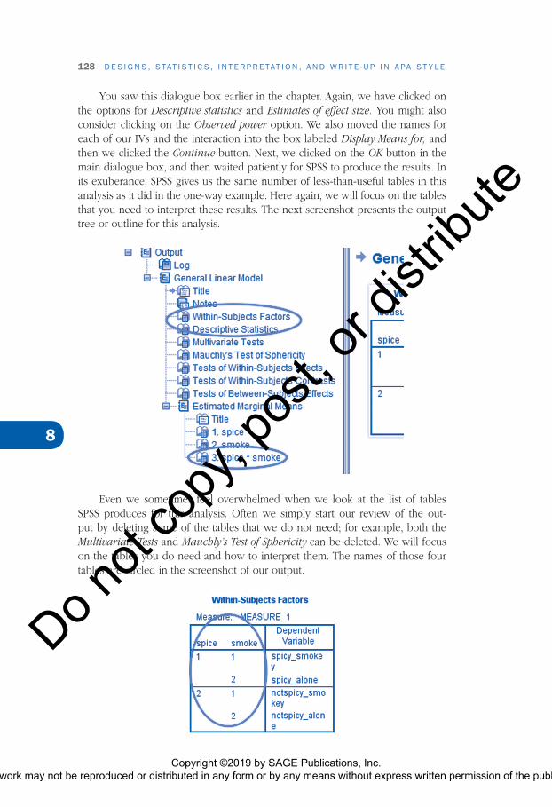
You saw this dialogue box earlier in the chapter. Again, we have clicked on the options for Descriptive statistics and Estimates of effect size. You might also consider clicking on the Observed power option. We also moved the names for each of our IVs and the interaction into the box labeled Display Means for, and then we clicked the Continue button. Next, we clicked on the OK button in the main dialogue box, and then waited patiently for SPSS to produce the results. In its exuberance, SPSS gives us the same number of less-than-useful tables in this analysis as it did in the one-way example. Here again, we will focus on the tables that you need to interpret these results. The next screenshot presents the output tree or outline for this analysis.

Even we sometimes feel overwhelmed when we look at the list of tables SPSS produces for this analysis. Often we simply start our review of the out-put by deleting some of the tables that we do not need; for example, both the Multivariate Tests and Mauchly’s Test of Sphericity can be deleted. We will focus on the tables you do need and how to interpret them. The names of those four tables are circled in the screenshot of our output.


Do not

copy

, pos

t, or d

istrib

ute


8

First, you should always look carefully at the Within-Subjects Factors table. This table can tell you if you entered your design correctly when you started the Repeated Measures procedure. In this example, we know we did because the circled labels match up with the names we placed in our design table three pages back. We wanted two levels for Spice and two levels for Smoke, and we can see that in the left-hand column in the following figure. Most important, you can see that the names for our DVs match up with those levels! The next table in the output presents the means and standard deviations for our conditions.

It is a good idea to review this table to see if the means and standard devia-tions are within the range that you expect based on previous research and your memory for how people responded in your experiment. You will see the means again in another table later in the output, and we will need them when we report our results in APA style.

Remember, we will skip the next two tables (Mauchly’s Test of Sphericity and Multivariate Tests) in the output. The Multivariate Tests are used for a differ-ent research design. (See Chapter 9 for an example of that design and analysis.) That brings us to the test of Within-Subjects Effects table. This one is the most important output table because it presents the results of our analysis of variance.


Do not

copy

, pos

t, or d

istrib

ute


8

Take a moment to look at the labels in the left-hand column. SPSS has pro-duced a pair of rows for both of the IVs and the interaction. You will notice that each of our IVs (e.g., Spice and Smoke) are paired with an error below it (e.g., Error(Spice) and Error(Smoke)). Now look at the next column of labels; you see that four labels repeat for each row in the table. We will focus on the rows labeled Sphericity Assumed. Again, the other rows are related to an advanced topic that is beyond the scope of this text. By this time you are familiar with the labels for the remaining columns in this table. They identify SS, df, Mean Square, F, p, and η2. To see if there were any significant effects, we look down the col-umn labeled Sig. to find our p values that are less than the .05 cutoff. In this case, we find that two of the values are in fact less than .001 (reported by SPSS as .000) and that the interaction has p = .017! So, we can conclude that there were signifi-cant differences in how much our volunteer tasters liked our chili based on the amount of spice, smoke, and the interaction of those two variables.

Next we want to look at the means representing each of those effects. We will look at the table for Spice first.

In the table labeled Spice, we see that they liked the spicy chili, M = 6.4, better than the not-spicy chili, M = 5.6. You can also find the 95% confidence intervals in case you need to report those or use them in the construction of a figure. The next table presents the results for the effect of Smoke.

In the table labeled Smoke, we find that the presence of smoke enhanced how much our volunteer tasters liked our chili, M = 6.3, compared with when it was tasted without smoke, M = 5.7. We must be careful in interpreting these two main effects because the interaction effect suggests a slightly more nuanced interpretation. The next table presents the descriptive statistics for that interaction.


Do not

copy

, pos

t, or d

istrib

ute


8

This final table presents our interaction. We wish that someone could teach SPSS to produce output for factorial designs in APA style. It would save us time and make it easier to interpret the output. Since no one has done that, we will have to work with the interaction table that is produced for us. You might need to take a moment to look back at the first table in this output to find out what the “1” and “2” under Spice and Smoke mean. In the next figure, we put the means for our four conditions in a design table like the one on page 126.

With that in mind, you might be able to see you can recast these means into an APA-style graph. We went ahead and did that, using Microsoft Excel to pro-duce the graph included here. Showing you how we did that is beyond the scope of this book. Finally, we will write this up in an APA-style summary.


ResultsWe used a 2(spice) × 2(smoke) within-subjects ANOVA on taste

ratings for our soon to be world famous chili. Participants rated the spicy chili (M = 6.4, SD = 2.4, n = 20) significantly more tasty than the mild (M = 5.6, SD = 2.4, n = 20), F(1, 19) = 39.78, p < .001, partial η2 = .68. They also significantly preferred the taste of both spice levels of chili when tasting with smoke in the air, F(1, 19) = 47.60, p <.001, partial η2 = .71. Most important, the two variables interacted to affect taste ratings, F(1, 19) = 6.78, p <.001, partial η2 = .26. We present the mean taste ratings, with 95% confidence intervals, for this interaction between spice and smoke in Figure 1. 0ur post hoc analyses showed that our participants liked both spicy and mild chili significantly more when they were tasted in the presence of smoke; however, the presence of smoke had a stronger effect for the mild chili.

6.60 6.20

6.10 5.15

Smoke Alone

Spicy

Not-Spicy


Do not

copy

, pos

t, or d

istrib

ute


8You should note that in our APA-style summary, we do not tell our read-

ers how we conducted the post hoc analyses to evaluate our interaction. In this case, we conducted two paired-samples t-tests. (This statistical test is the first one described in this chapter.) The first compared taste ratings of our spicy chili with and without smoke in the air. The second compared taste ratings of our mild chili with and without smoke in the air. Our general finding is that smoke has a stronger effect on appreciation for the milder chili.

Based on this analysis, we would open our restaurant and serve both kinds of chili, but we would tell our customers that they are likely to enjoy the spicy chili more than the mild. We would have a wood-burning fireplace or oven so that people would enjoy our chili more but especially the mild version.

Summary

At this point, you should know how to conduct the statistical analyses that are most commonly used for data collected in repeated-measures designs, starting with simple two-level designs and ending with factorial design. Remember that each of these can be expanded to include more levels or more variables. In the next chapter, you can learn about the analysis of data collected in some more complicated research designs.

Figure 1 Means With 95% Confidence Intervals for Taste Ratings of Spicy and Mild Chili Tasted Under Smokey and Not Smokey Conditions

9

8

7

6

5

4

3

2

1

0Smoke

Mea

n T

aste

Rat

ing

Alone

Spicy Not-Spicy


Do not

copy

, pos

t, or d

istrib

ute

repeated- measures 8 designs · designs, statistics, interpretation, and write-up in apa style. 8....

Documents