Two-Factor Repeated Measures Designs

James H. Steiger

Department of Psychology and Human DevelopmentVanderbilt University

James H. Steiger (Vanderbilt University) 1 / 14

Two-Factor Repeated Measures Designs1 Introduction

2 The S × A× B Within-Subjects Design

Introduction

Melting and Reshaping the Data

Analyzing with ezANOVA

3 The S × A× B Between-Within Design

Introduction

Reading and Reshaping the Data

James H. Steiger (Vanderbilt University) 2 / 14

Introduction

In previous modules, we discovered that the completely randomizeddesign and the randomized blocks design are fundamental buildingblocks for a number of other designs.

We also pointed out that the 1-Way Repeated Measures design isactually a randomized blocks design with Subjects as the singleblocking factor.

In this module, we explore extensions of the basic designs.

The extensions can go in several directions:

1 There can be more than one repeated measure, or within-subjectsfactor.

2 In a repeated measures design, there can be more than one group ofsubjects, in which case we have a between-subjects factor. Indeed,there can be several between-subjects factors combined factorially.

3 When within-subjects and between-subjects factors occur in the samedesign, we can refer to the design as a between-within design.

James H. Steiger (Vanderbilt University) 3 / 14

Introduction

In previous modules, we discovered that the completely randomizeddesign and the randomized blocks design are fundamental buildingblocks for a number of other designs.

We also pointed out that the 1-Way Repeated Measures design isactually a randomized blocks design with Subjects as the singleblocking factor.

In this module, we explore extensions of the basic designs.

The extensions can go in several directions:

1 There can be more than one repeated measure, or within-subjectsfactor.

2 In a repeated measures design, there can be more than one group ofsubjects, in which case we have a between-subjects factor. Indeed,there can be several between-subjects factors combined factorially.

3 When within-subjects and between-subjects factors occur in the samedesign, we can refer to the design as a between-within design.

James H. Steiger (Vanderbilt University) 3 / 14

Introduction

In previous modules, we discovered that the completely randomizeddesign and the randomized blocks design are fundamental buildingblocks for a number of other designs.

We also pointed out that the 1-Way Repeated Measures design isactually a randomized blocks design with Subjects as the singleblocking factor.

In this module, we explore extensions of the basic designs.

The extensions can go in several directions:

1 There can be more than one repeated measure, or within-subjectsfactor.

2 In a repeated measures design, there can be more than one group ofsubjects, in which case we have a between-subjects factor. Indeed,there can be several between-subjects factors combined factorially.

3 When within-subjects and between-subjects factors occur in the samedesign, we can refer to the design as a between-within design.

James H. Steiger (Vanderbilt University) 3 / 14

Introduction

In previous modules, we discovered that the completely randomizeddesign and the randomized blocks design are fundamental buildingblocks for a number of other designs.

We also pointed out that the 1-Way Repeated Measures design isactually a randomized blocks design with Subjects as the singleblocking factor.

In this module, we explore extensions of the basic designs.

The extensions can go in several directions:

1 There can be more than one repeated measure, or within-subjectsfactor.

2 In a repeated measures design, there can be more than one group ofsubjects, in which case we have a between-subjects factor. Indeed,there can be several between-subjects factors combined factorially.

3 When within-subjects and between-subjects factors occur in the samedesign, we can refer to the design as a between-within design.

James H. Steiger (Vanderbilt University) 3 / 14

Introduction

In previous modules, we discovered that the completely randomizeddesign and the randomized blocks design are fundamental buildingblocks for a number of other designs.

We also pointed out that the 1-Way Repeated Measures design isactually a randomized blocks design with Subjects as the singleblocking factor.

In this module, we explore extensions of the basic designs.

The extensions can go in several directions:

1 There can be more than one repeated measure, or within-subjectsfactor.

2 In a repeated measures design, there can be more than one group ofsubjects, in which case we have a between-subjects factor. Indeed,there can be several between-subjects factors combined factorially.

3 When within-subjects and between-subjects factors occur in the samedesign, we can refer to the design as a between-within design.

James H. Steiger (Vanderbilt University) 3 / 14

Introduction

In previous modules, we discovered that the completely randomizeddesign and the randomized blocks design are fundamental buildingblocks for a number of other designs.

We also pointed out that the 1-Way Repeated Measures design isactually a randomized blocks design with Subjects as the singleblocking factor.

In this module, we explore extensions of the basic designs.

The extensions can go in several directions:

1 There can be more than one repeated measure, or within-subjectsfactor.

2 In a repeated measures design, there can be more than one group ofsubjects, in which case we have a between-subjects factor. Indeed,there can be several between-subjects factors combined factorially.

3 When within-subjects and between-subjects factors occur in the samedesign, we can refer to the design as a between-within design.

James H. Steiger (Vanderbilt University) 3 / 14

Introduction

In previous modules, we discovered that the completely randomizeddesign and the randomized blocks design are fundamental buildingblocks for a number of other designs.

We also pointed out that the 1-Way Repeated Measures design isactually a randomized blocks design with Subjects as the singleblocking factor.

In this module, we explore extensions of the basic designs.

The extensions can go in several directions:

1 There can be more than one repeated measure, or within-subjectsfactor.

2 In a repeated measures design, there can be more than one group ofsubjects, in which case we have a between-subjects factor. Indeed,there can be several between-subjects factors combined factorially.

3 When within-subjects and between-subjects factors occur in the samedesign, we can refer to the design as a between-within design.

James H. Steiger (Vanderbilt University) 3 / 14

The S × A × B Within-Subjects Design Introduction

The S × A× B Within-Subjects DesignIntroduction

We can extend the 1-Way Repeated Measures design to two or morerepeated measures factors, combined factorially.

An example is presented in RDASA3 Section 15.2.

Each of 6 subjects were presented with figures that were varied across3 levels of Distortion (Factor A) and 3 levels of Orientation (FactorB). So each subject was presented with 9 photos in all. The order ofpresentation was varied randomly for each subject.

Data are presented in Table 15.3, and are available online in the fileTable1503.csv.

James H. Steiger (Vanderbilt University) 4 / 14

The S × A × B Within-Subjects Design Introduction

The S × A× B Within-Subjects DesignIntroduction

James H. Steiger (Vanderbilt University) 5 / 14

The S × A × B Within-Subjects Design Introduction

The S × A× B Within-Subjects DesignIntroduction

As is usually the case with repeated measures data, we need to recastthe data prior to analysis. We start by reading in the data and addinga Subject variable.

> Table1503 <- read.csv("Table1503.csv")

> Subject <- 1:6

> Table1503 <- cbind(Subject, Table1503)

> Table1503

Subject A1B1 A2B1 A3B1 A1B2 A2B2 A3B2 A1B3 A2B3 A3B3

1 1 1.18 2.40 2.48 4.76 4.93 3.13 5.56 4.93 5.21

2 2 1.14 1.55 1.25 4.81 4.73 3.89 4.85 5.43 4.89

3 3 1.02 1.25 1.30 4.98 3.85 3.05 4.28 5.64 6.49

4 4 1.05 1.63 1.84 4.91 5.21 2.95 5.13 5.52 5.69

5 5 1.81 1.65 1.01 5.01 4.18 3.51 4.90 5.18 5.52

6 6 1.69 1.67 1.04 5.65 4.56 3.94 4.12 5.76 4.99

James H. Steiger (Vanderbilt University) 6 / 14

The S × A × B Within-Subjects Design Melting and Reshaping the Data

The S × A× B Within-Subjects DesignMelting the Data

Next, we “melt” the data, using the melt function from the reshape

library.

Note how, in the call, I just use the numbers of the variables to beused as id.vars and measured.vars.

> temp <- melt(Table1503, id.vars = 1, measure.vars = 2:10)

> temp[1:10, ]

Subject variable value

1 1 A1B1 1.18

2 2 A1B1 1.14

3 3 A1B1 1.02

4 4 A1B1 1.05

5 5 A1B1 1.81

6 6 A1B1 1.69

7 1 A2B1 2.40

8 2 A2B1 1.55

9 3 A2B1 1.25

10 4 A2B1 1.63

Taking a look at this, we see that R still has no way of knowing howto identify which columns stand for which factors, and which levelsare involved.

Thorough study of the reshape package and the (different) reshape

function in R may well enable you to automate the further processingof the data. In this case, I simply create new variables to tell R whichobservations are at which levels of each factor.

Code on the next slide shows how I did this.

James H. Steiger (Vanderbilt University) 7 / 14

The S × A × B Within-Subjects Design Melting and Reshaping the Data

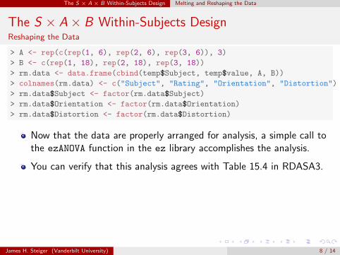
The S × A× B Within-Subjects DesignReshaping the Data

> A <- rep(c(rep(1, 6), rep(2, 6), rep(3, 6)), 3)

> B <- c(rep(1, 18), rep(2, 18), rep(3, 18))

> rm.data <- data.frame(cbind(temp$Subject, temp$value, A, B))

> colnames(rm.data) <- c("Subject", "Rating", "Orientation", "Distortion")

> rm.data$Subject <- factor(rm.data$Subject)

> rm.data$Orientation <- factor(rm.data$Orientation)

> rm.data$Distortion <- factor(rm.data$Distortion)

Now that the data are properly arranged for analysis, a simple call tothe ezANOVA function in the ez library accomplishes the analysis.

You can verify that this analysis agrees with Table 15.4 in RDASA3.

James H. Steiger (Vanderbilt University) 8 / 14

The S × A × B Within-Subjects Design Analyzing with ezANOVA

The S × A× B Within-Subjects DesignAnalyzing with ezANOVA

> ezANOVA(rm.data, wid = .(Subject), dv = .(Rating), within = .(Orientation, Distortion))

$ANOVA

Effect DFn DFd F p p<.05 ges

2 Orientation 2 10 9.233704 5.348849e-03 * 0.1586956

3 Distortion 2 10 302.559959 1.135536e-09 * 0.9364271

4 Orientation:Distortion 4 20 7.750117 6.088323e-04 * 0.4800754

$`Mauchly's Test for Sphericity`

Effect W p p<.05

2 Orientation 0.96186281 0.9251801

3 Distortion 0.92723232 0.8597598

4 Orientation:Distortion 0.05631215 0.4226226

$`Sphericity Corrections`

Effect GGe p[GG] p[GG]<.05 HFe

2 Orientation 0.9632638 6.038310e-03 * 1.5551085

3 Distortion 0.9321683 3.939469e-09 * 1.4647649

4 Orientation:Distortion 0.4617494 1.149319e-02 * 0.7201061

p[HF] p[HF]<.05

2 5.348849e-03 *

3 1.135536e-09 *

4 2.753985e-03 *

James H. Steiger (Vanderbilt University) 9 / 14

The S × A × B Within-Subjects Design Analyzing with ezANOVA

The S × A× B Within-Subjects DesignAnalyzing with ezANOVA

James H. Steiger (Vanderbilt University) 10 / 14

The S × A × B Between-Within Design Introduction

The S × A× B Between-Within DesignIntroduction

A frequently-used design is the S ×A×B between-within design, withthe A and B fixed effects factors crossed factorially, but with differentgroups of subjects in each cell representing the levels of the A factor,but each subject being measured on all levels of the B factor.

I prefer to call such a design a “between-within” design.

MWL refer to it as a “mixed” design, a poor choice because it iseasily confused with a “mixed model” (meaning random effects andfixed effects in the same design. I’ll stick to the term“between-within” when describing such models.

An example of data for such a design is shown in RDASA3, Figure15.5.

James H. Steiger (Vanderbilt University) 11 / 14

The S × A × B Between-Within Design Introduction

The S × A× B Between-Within DesignIntroduction

A frequently-used design is the S ×A×B between-within design, withthe A and B fixed effects factors crossed factorially, but with differentgroups of subjects in each cell representing the levels of the A factor,but each subject being measured on all levels of the B factor.

I prefer to call such a design a “between-within” design.

MWL refer to it as a “mixed” design, a poor choice because it iseasily confused with a “mixed model” (meaning random effects andfixed effects in the same design. I’ll stick to the term“between-within” when describing such models.

An example of data for such a design is shown in RDASA3, Figure15.5.

James H. Steiger (Vanderbilt University) 11 / 14

The S × A × B Between-Within Design Introduction

The S × A× B Between-Within DesignIntroduction

A frequently-used design is the S ×A×B between-within design, withthe A and B fixed effects factors crossed factorially, but with differentgroups of subjects in each cell representing the levels of the A factor,but each subject being measured on all levels of the B factor.

I prefer to call such a design a “between-within” design.

MWL refer to it as a “mixed” design, a poor choice because it iseasily confused with a “mixed model” (meaning random effects andfixed effects in the same design. I’ll stick to the term“between-within” when describing such models.

An example of data for such a design is shown in RDASA3, Figure15.5.

James H. Steiger (Vanderbilt University) 11 / 14

The S × A × B Between-Within Design Introduction

The S × A× B Between-Within DesignIntroduction

A frequently-used design is the S ×A×B between-within design, withthe A and B fixed effects factors crossed factorially, but with differentgroups of subjects in each cell representing the levels of the A factor,but each subject being measured on all levels of the B factor.

I prefer to call such a design a “between-within” design.

MWL refer to it as a “mixed” design, a poor choice because it iseasily confused with a “mixed model” (meaning random effects andfixed effects in the same design. I’ll stick to the term“between-within” when describing such models.

An example of data for such a design is shown in RDASA3, Figure15.5.

James H. Steiger (Vanderbilt University) 11 / 14

The S × A × B Between-Within Design Introduction

The S × A× B Between-Within DesignIntroduction

James H. Steiger (Vanderbilt University) 12 / 14

The S × A × B Between-Within Design Reading and Reshaping the Data

The S × A× B Between-Within DesignReading and Reshaping the Data

> Table1505 <- read.csv("Table1505.csv")

> rm.data <- data.frame(melt(Table1505, id.vars = 1:2, measure.vars = 3:6))

> rm.data$A <- factor(rm.data$A)

> rm.data$Subject <- factor(rm.data$Subject)

> colnames(rm.data) = c("Subject", "Method", "Time", "Score")

> rm.data[1:12, ]

Subject Method Time Score

1 1 1 B1 82

2 2 1 B1 72

3 3 1 B1 43

4 4 1 B1 77

5 5 1 B1 43

6 6 1 B1 67

7 7 2 B1 71

8 8 2 B1 89

9 9 2 B1 82

10 10 2 B1 56

11 11 2 B1 64

12 12 2 B1 76

James H. Steiger (Vanderbilt University) 13 / 14

The S × A × B Between-Within Design Reading and Reshaping the Data

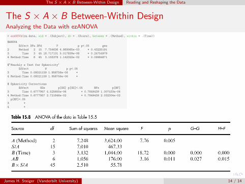
The S × A× B Between-Within DesignAnalyzing the Data with ezANOVA

> ezANOVA(rm.data, wid = .(Subject), dv = .(Score), between = .(Method), within = .(Time))

$ANOVA

Effect DFn DFd F p p<.05 ges

2 Method 2 15 7.754636 4.869065e-03 * 0.43225191

3 Time 3 45 18.717131 5.017839e-08 * 0.24754979

4 Method:Time 6 45 3.155378 1.142322e-02 * 0.09984871

$`Mauchly's Test for Sphericity`

Effect W p p<.05

3 Time 0.08021159 1.958756e-06 *

4 Method:Time 0.08021159 1.958756e-06 *

$`Sphericity Corrections`

Effect GGe p[GG] p[GG]<.05 HFe p[HF]

3 Time 0.6777957 4.525655e-06 * 0.7849439 1.007433e-06

4 Method:Time 0.6777957 2.721846e-02 * 0.7849439 2.032304e-02

p[HF]<.05

3 *

4 *

James H. Steiger (Vanderbilt University) 14 / 14