one-factor repeated measures design notes/ch14.pdf · a repeated measures analysis of seasonal...
TRANSCRIPT

IntroductionThe Nonadditive Model for the S × A Design
The Sphericity AssumptionA Repeated Measures Analysis of Seasonal DepressionAnalyzing Repeated Measures with Hotelling’s T2
One-Factor Repeated Measures Design
James H. Steiger
Department of Psychology and Human DevelopmentVanderbilt University
P311, 2012
James H. Steiger One-Factor Repeated Measures Design
IntroductionThe Nonadditive Model for the S × A Design
The Sphericity AssumptionA Repeated Measures Analysis of Seasonal DepressionAnalyzing Repeated Measures with Hotelling’s T2
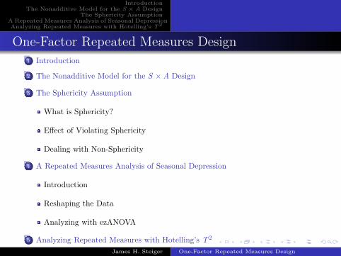
One-Factor Repeated Measures Design1 Introduction
2 The Nonadditive Model for the S ×A Design
3 The Sphericity Assumption
What is Sphericity?
Effect of Violating Sphericity
Dealing with Non-Sphericity
4 A Repeated Measures Analysis of Seasonal Depression
Introduction
Reshaping the Data
Analyzing with ezANOVA
5 Analyzing Repeated Measures with Hotelling’s T 2
James H. Steiger One-Factor Repeated Measures Design

IntroductionThe Nonadditive Model for the S × A Design
The Sphericity AssumptionA Repeated Measures Analysis of Seasonal DepressionAnalyzing Repeated Measures with Hotelling’s T2
One-Factor Repeated Measures DesignIntroduction
In the one-way repeated measures design, n randomlysampled subjects are measured repeatedly on a occasions.This is sometimes called the “subjects by trials” design forthat reason.In the previous module, we discussed the randomized blocksdesign, which is in fact a special case of a mixed-effectstwo-way ANOVA, with 1 observation per cell, or a unitsper block.I pointed out that, when the “block size” is a, the aobservations can be either different individuals matched byblocking, or repeated measurements on the sameobservational unit or subject.The one-way repeated measures design that employs the“nonadditive model” and assumes that the blocking factor(i.e., “Subjects”) is a random effect, is identical to therandomized blocks model with a fixed effect treatment andone observation per cell that we examined earlier.The “additive model” discussed by MWS in section 14.2 ofRDASA3 seems unrealistic. It assumes that the effect overrepeated measures is the same for all subjects. I will notdiscuss it further here.
James H. Steiger One-Factor Repeated Measures Design

IntroductionThe Nonadditive Model for the S × A Design
The Sphericity AssumptionA Repeated Measures Analysis of Seasonal DepressionAnalyzing Repeated Measures with Hotelling’s T2
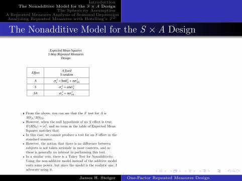
The Nonadditive Model for the S × A Design
The additive model for the S ×A design is essentially thesame as for the randomized blocks RB-p design, which is inturn a mixed model ANOVA.The “Subjects” (S ) factor is considered random, and the“Trials” factor (A) is fixed.You will note that the description of the model in RDASA3Section 14.5.1 is incomplete in several respects.The Expected Mean Squares and F ratios for thenon-additive model are given on the next slide. You willrecognize them as equivalent to the values given for a2-way mixed model randomized factorial design with onefactor fixed and the other random.
James H. Steiger One-Factor Repeated Measures Design
IntroductionThe Nonadditive Model for the S × A Design
The Sphericity AssumptionA Repeated Measures Analysis of Seasonal DepressionAnalyzing Repeated Measures with Hotelling’s T2
The Nonadditive Model for the S × A Design
The additive model for the S ×A design is essentially thesame as for the randomized blocks RB-p design, which is inturn a mixed model ANOVA.The “Subjects” (S ) factor is considered random, and the“Trials” factor (A) is fixed.You will note that the description of the model in RDASA3Section 14.5.1 is incomplete in several respects.The Expected Mean Squares and F ratios for thenon-additive model are given on the next slide. You willrecognize them as equivalent to the values given for a2-way mixed model randomized factorial design with onefactor fixed and the other random.
James H. Steiger One-Factor Repeated Measures Design
IntroductionThe Nonadditive Model for the S × A Design
The Sphericity AssumptionA Repeated Measures Analysis of Seasonal DepressionAnalyzing Repeated Measures with Hotelling’s T2
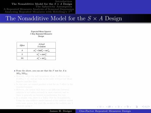
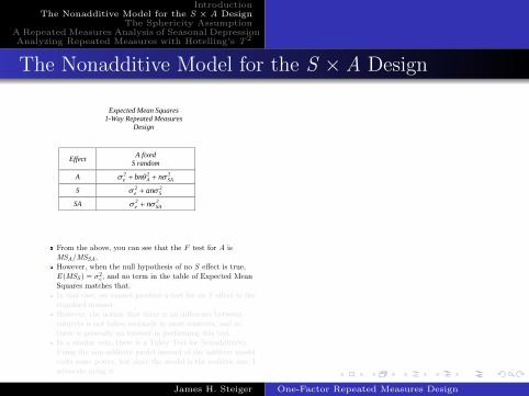
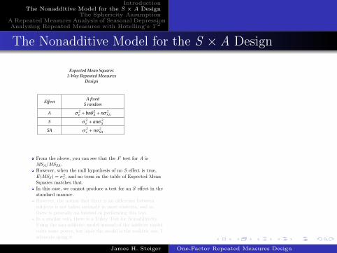
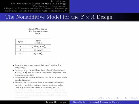
The Nonadditive Model for the S × A Design
Expected Mean Squares 1-Way Repeated Measures
Design
Effect A fixed S random
A 2 2 2e A SAnbnσ θ σ++
S 2 2e Sanσ σ+
SA 2 2e SAnσ σ+
From the above, you can see that the F test for A isMSA/MSSA.However, when the null hypothesis of no S effect is true,E (MSS ) = σ2e , and no term in the table of Expected MeanSquares matches that.In this case, we cannot produce a test for an S effect in thestandard manner.However, the notion that there is no difference betweensubjects is not taken seriously in most contexts, and sothere is generally no interest in performing this test.In a similar vein, there is a Tukey Test for Nonadditivity.Using the non-additive model instead of the additive modelcosts some power, but since the model is the realistic one, Iadvocate using it.
James H. Steiger One-Factor Repeated Measures Design
IntroductionThe Nonadditive Model for the S × A Design
The Sphericity AssumptionA Repeated Measures Analysis of Seasonal DepressionAnalyzing Repeated Measures with Hotelling’s T2
What is Sphericity?Effect of Violating SphericityDealing with Non-Sphericity
The Sphericity Assumption
We recall from our earlier discussions that ANOVA involvesan assumption of equal variances.In repeated measures designs, an additional assumption ofsphericity is required.This assumption states that, if we consider all levels of therandom effects variable, and compute all pairwisedifferences between these levels, they must have equalvariance.Note that, if there are a levels of the treatment, then thereare
(a2
)= a(a − 1)/2 differences to be calculated.
James H. Steiger One-Factor Repeated Measures Design
IntroductionThe Nonadditive Model for the S × A Design
The Sphericity AssumptionA Repeated Measures Analysis of Seasonal DepressionAnalyzing Repeated Measures with Hotelling’s T2
What is Sphericity?Effect of Violating SphericityDealing with Non-Sphericity
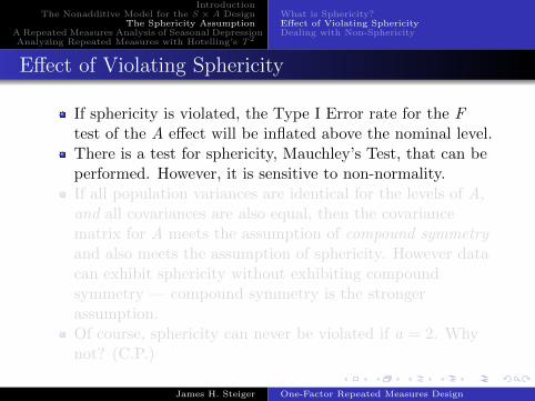
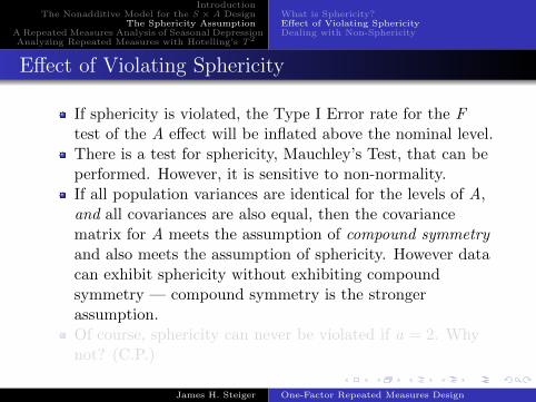
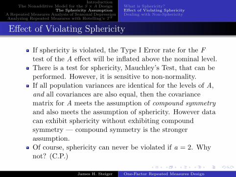
Effect of Violating Sphericity
If sphericity is violated, the Type I Error rate for the Ftest of the A effect will be inflated above the nominal level.There is a test for sphericity, Mauchley’s Test, that can beperformed. However, it is sensitive to non-normality.If all population variances are identical for the levels of A,and all covariances are also equal, then the covariancematrix for A meets the assumption of compound symmetryand also meets the assumption of sphericity. However datacan exhibit sphericity without exhibiting compoundsymmetry — compound symmetry is the strongerassumption.Of course, sphericity can never be violated if a = 2. Whynot? (C.P.)
James H. Steiger One-Factor Repeated Measures Design
IntroductionThe Nonadditive Model for the S × A Design
The Sphericity AssumptionA Repeated Measures Analysis of Seasonal DepressionAnalyzing Repeated Measures with Hotelling’s T2
What is Sphericity?Effect of Violating SphericityDealing with Non-Sphericity
Effect of Violating Sphericity
If sphericity is violated, the Type I Error rate for the Ftest of the A effect will be inflated above the nominal level.There is a test for sphericity, Mauchley’s Test, that can beperformed. However, it is sensitive to non-normality.If all population variances are identical for the levels of A,and all covariances are also equal, then the covariancematrix for A meets the assumption of compound symmetryand also meets the assumption of sphericity. However datacan exhibit sphericity without exhibiting compoundsymmetry — compound symmetry is the strongerassumption.Of course, sphericity can never be violated if a = 2. Whynot? (C.P.)
James H. Steiger One-Factor Repeated Measures Design

IntroductionThe Nonadditive Model for the S × A Design
The Sphericity AssumptionA Repeated Measures Analysis of Seasonal DepressionAnalyzing Repeated Measures with Hotelling’s T2
What is Sphericity?Effect of Violating SphericityDealing with Non-Sphericity
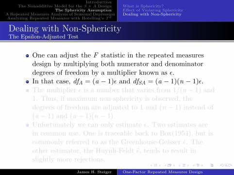
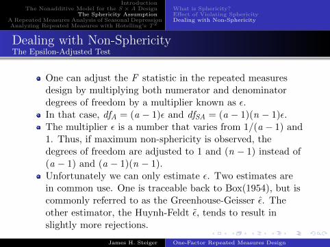
Dealing with Non-SphericityThe Epsilon-Adjusted Test
One can adjust the F statistic in the repeated measuresdesign by multiplying both numerator and denominatordegrees of freedom by a multiplier known as ε.In that case, dfA = (a − 1)ε and dfSA = (a − 1)(n − 1)ε.The multiplier ε is a number that varies from 1/(a − 1) and1. Thus, if maximum non-sphericity is observed, thedegrees of freedom are adjusted to 1 and (n − 1) instead of(a − 1) and (a − 1)(n − 1).Unfortunately we can only estimate ε. Two estimates arein common use. One is traceable back to Box(1954), but iscommonly referred to as the Greenhouse-Geisser ε̂. Theother estimator, the Huynh-Feldt ε̃, tends to result inslightly more rejections.
James H. Steiger One-Factor Repeated Measures Design
IntroductionThe Nonadditive Model for the S × A Design
The Sphericity AssumptionA Repeated Measures Analysis of Seasonal DepressionAnalyzing Repeated Measures with Hotelling’s T2
What is Sphericity?Effect of Violating SphericityDealing with Non-Sphericity
Dealing with Non-SphericityThe Epsilon-Adjusted Test
One can adjust the F statistic in the repeated measuresdesign by multiplying both numerator and denominatordegrees of freedom by a multiplier known as ε.In that case, dfA = (a − 1)ε and dfSA = (a − 1)(n − 1)ε.The multiplier ε is a number that varies from 1/(a − 1) and1. Thus, if maximum non-sphericity is observed, thedegrees of freedom are adjusted to 1 and (n − 1) instead of(a − 1) and (a − 1)(n − 1).Unfortunately we can only estimate ε. Two estimates arein common use. One is traceable back to Box(1954), but iscommonly referred to as the Greenhouse-Geisser ε̂. Theother estimator, the Huynh-Feldt ε̃, tends to result inslightly more rejections.
James H. Steiger One-Factor Repeated Measures Design
IntroductionThe Nonadditive Model for the S × A Design
The Sphericity AssumptionA Repeated Measures Analysis of Seasonal DepressionAnalyzing Repeated Measures with Hotelling’s T2
IntroductionReshaping the DataAnalyzing with ezANOVA
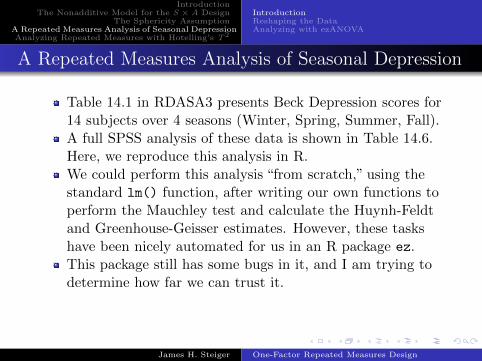
A Repeated Measures Analysis of Seasonal Depression
Table 14.1 in RDASA3 presents Beck Depression scores for14 subjects over 4 seasons (Winter, Spring, Summer, Fall).A full SPSS analysis of these data is shown in Table 14.6.Here, we reproduce this analysis in R.We could perform this analysis “from scratch,” using thestandard lm() function, after writing our own functions toperform the Mauchley test and calculate the Huynh-Feldtand Greenhouse-Geisser estimates. However, these taskshave been nicely automated for us in an R package ez.This package still has some bugs in it, and I am trying todetermine how far we can trust it.
James H. Steiger One-Factor Repeated Measures Design
IntroductionThe Nonadditive Model for the S × A Design
The Sphericity AssumptionA Repeated Measures Analysis of Seasonal DepressionAnalyzing Repeated Measures with Hotelling’s T2
IntroductionReshaping the DataAnalyzing with ezANOVA
A Repeated Measures Analysis of Seasonal Depression
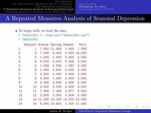
To begin with, we load the data
> Table1401 <- read.csv("Table1401.csv")
> Table1401
Subject Winter Spring Summer Fall
1 1 7.500 11.554 1.000 1.208
2 2 7.000 9.000 5.000 15.000
3 3 1.000 1.000 0.000 0.000
4 4 0.000 0.000 0.000 0.000
5 5 1.059 0.000 1.097 4.000
6 6 1.000 2.500 0.000 2.000
7 7 2.500 0.000 0.000 2.000
8 8 4.500 1.060 2.000 2.000
9 9 5.000 2.000 3.000 5.000
10 10 2.000 3.000 4.208 3.000
11 11 7.000 7.354 5.877 9.000
12 12 2.500 2.000 0.009 2.000
13 13 11.000 16.000 13.000 13.000
14 14 8.000 10.500 1.000 11.000
James H. Steiger One-Factor Repeated Measures Design

IntroductionThe Nonadditive Model for the S × A Design
The Sphericity AssumptionA Repeated Measures Analysis of Seasonal DepressionAnalyzing Repeated Measures with Hotelling’s T2
IntroductionReshaping the DataAnalyzing with ezANOVA
A Repeated Measures Analysis of Seasonal DepressionReshaping the Data
This format seems natural for the data — one line for eachsubject.Unfortunately, this is not the format typically required byanalysis of variance routines, because in this case, thesubject is being treated as a level of the Subject (S ) factorin the design, and each column is a repeated measure thatis treated as a level of the A factor.In effect, then, we have a S ×A, 14 × 4 ANOVA with 1observation per cell, and the data need to be recast thatway. How?Well, we could do it by hand, or we could write a briefprogram in R to do it. This is a skill we’ll need to master,especially if we do repeated measures ANOVAs often.There is another way. We can use a library, reshape,designed especially for this task.
James H. Steiger One-Factor Repeated Measures Design
IntroductionThe Nonadditive Model for the S × A Design
The Sphericity AssumptionA Repeated Measures Analysis of Seasonal DepressionAnalyzing Repeated Measures with Hotelling’s T2
IntroductionReshaping the DataAnalyzing with ezANOVA
A Repeated Measures Analysis of Seasonal DepressionReshaping the Data
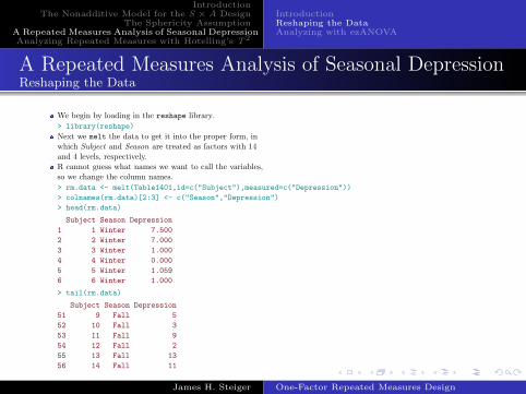
We begin by loading in the reshape library.
> library(reshape)
Next we melt the data to get it into the proper form, inwhich Subject and Season are treated as factors with 14and 4 levels, respectively.R cannot guess what names we want to call the variables,so we change the column names.
> rm.data <- melt(Table1401,id=c("Subject"),measured=c("Depression"))
> colnames(rm.data)[2:3] <- c("Season","Depression")
> head(rm.data)
Subject Season Depression
1 1 Winter 7.500
2 2 Winter 7.000
3 3 Winter 1.000
4 4 Winter 0.000
5 5 Winter 1.059
6 6 Winter 1.000
> tail(rm.data)
Subject Season Depression
51 9 Fall 5
52 10 Fall 3
53 11 Fall 9
54 12 Fall 2
55 13 Fall 13
56 14 Fall 11
James H. Steiger One-Factor Repeated Measures Design
IntroductionThe Nonadditive Model for the S × A Design
The Sphericity AssumptionA Repeated Measures Analysis of Seasonal DepressionAnalyzing Repeated Measures with Hotelling’s T2
IntroductionReshaping the DataAnalyzing with ezANOVA
Analyzing with ezANOVA
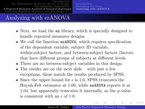
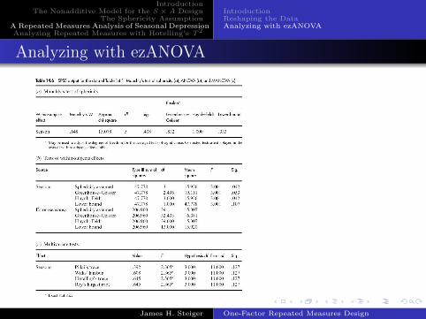
Next, we load the ez library, which is specially designed tohandle repeated measures designs.We call the function ezANOVA, which requires specificationof the dependent variable, subject ID variable,within-subject factors, and between-subject factors (factorsthat have different groups of subjects at different levels.There are no between-subject variables in this design.The results are on the next slide – with just a fewexceptions, these match the results produced by SPSS.Since the upper bound for ε is 1.0, SPSS truncates theHuynh-Felt estimator at 1.00, while ezANOVA reports it at1.04, but apparently truncates it internally, as the p-valueis consistent with an ε of 1.0.
James H. Steiger One-Factor Repeated Measures Design
IntroductionThe Nonadditive Model for the S × A Design
The Sphericity AssumptionA Repeated Measures Analysis of Seasonal DepressionAnalyzing Repeated Measures with Hotelling’s T2
IntroductionReshaping the DataAnalyzing with ezANOVA
Analyzing with ezANOVA
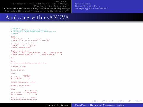
> library(ez)
> results <-ezANOVA(data=rm.data,dv=.(Depression),
+ wid=.(Subject),within=.(Season),type="III",return_aov=TRUE)
> results
$ANOVA
Effect DFn DFd F p p<.05 ges
2 Season 3 39 3.00115 0.04202195 * 0.04621462
$`Mauchly's Test for Sphericity`
Effect W p p<.05
2 Season 0.648444 0.4078981
$`Sphericity Corrections`
Effect GGe p[GG] p[GG]<.05 HFe p[HF] p[HF]<.05
2 Season 0.8316087 0.05321143 1.044805 0.04202195 *
$aov
Call:
aov(formula = formula(aov_formula), data = data)
Grand Mean: 4.132607
Stratum 1: Subject
Terms:
Residuals
Sum of Squares 779.0988
Deg. of Freedom 13
Residual standard error: 7.741491
Stratum 2: Subject:Season
Terms:
Season Residuals
Sum of Squares 47.77842 206.96047
Deg. of Freedom 3 39
Residual standard error: 2.303623
Estimated effects may be unbalanced
James H. Steiger One-Factor Repeated Measures Design
IntroductionThe Nonadditive Model for the S × A Design
The Sphericity AssumptionA Repeated Measures Analysis of Seasonal DepressionAnalyzing Repeated Measures with Hotelling’s T2
IntroductionReshaping the DataAnalyzing with ezANOVA
Analyzing with ezANOVA
James H. Steiger One-Factor Repeated Measures Design
IntroductionThe Nonadditive Model for the S × A Design
The Sphericity AssumptionA Repeated Measures Analysis of Seasonal DepressionAnalyzing Repeated Measures with Hotelling’s T2
A Multivariate Approach
Strictly speaking, repeated measures data are multivariate,in that each subject (or unit of observation) producesseveral responses.The ANOVA approach to repeated measures requires thestrong assumption of sphericity in order to reduce amultivariate problem to a univariate problem.An alternate approach is to use a truly multivariateapproach, that allows the data to have any populationcovariance structure.This approach is actually a generalization of the univariatet test called Hotelling’s T 2.
James H. Steiger One-Factor Repeated Measures Design
IntroductionThe Nonadditive Model for the S × A Design
The Sphericity AssumptionA Repeated Measures Analysis of Seasonal DepressionAnalyzing Repeated Measures with Hotelling’s T2
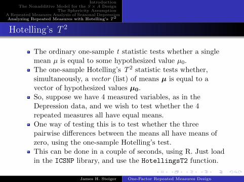
Hotelling’s T 2
The ordinary one-sample t statistic tests whether a singlemean µ is equal to some hypothesized value µ0.The one-sample Hotelling’s T 2 statistic tests whether,simultaneously, a vector (list) of means µ is equal to avector of hypothesized values µ0.So, suppose we have 4 measured variables, as in theDepression data, and we wish to test whether the 4repeated measures all have equal means.One way of testing this is to test whether the threepairwise differences between the means all have means ofzero, using the one-sample Hotelling’s test.This can be done in a couple of seconds, using R. Just loadin the ICSNP library, and use the HotellingsT2 function.
James H. Steiger One-Factor Repeated Measures Design
IntroductionThe Nonadditive Model for the S × A Design
The Sphericity AssumptionA Repeated Measures Analysis of Seasonal DepressionAnalyzing Repeated Measures with Hotelling’s T2
Hotelling’s T 2
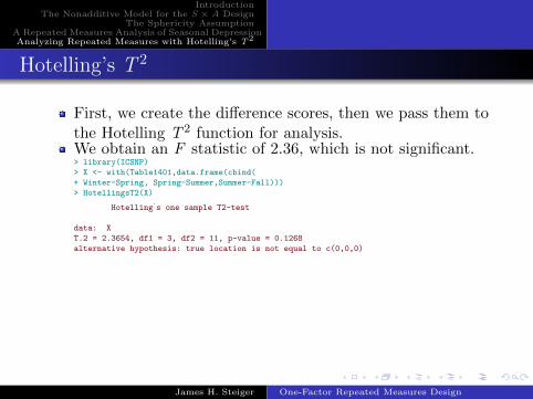
First, we create the difference scores, then we pass them tothe Hotelling T 2 function for analysis.We obtain an F statistic of 2.36, which is not significant.> library(ICSNP)
> X <- with(Table1401,data.frame(cbind(
+ Winter-Spring, Spring-Summer,Summer-Fall)))
> HotellingsT2(X)
Hotelling's one sample T2-test
data: X
T.2 = 2.3654, df1 = 3, df2 = 11, p-value = 0.1268
alternative hypothesis: true location is not equal to c(0,0,0)
James H. Steiger One-Factor Repeated Measures Design