repeated measures analysis - ncss · this module calculates the power for repeated measures ... an...
TRANSCRIPT
PASS Sample Size Software NCSS.com
570-1 © NCSS, LLC. All Rights Reserved.
Chapter 570
Repeated Measures Analysis Introduction This module calculates the power for repeated measures designs having up to three between factors and up to three within factors. It computes power for both the univariate (F test and F test with Geisser-Greenhouse correction) and multivariate (Wilks’ lambda, Pillai-Bartlett trace, and Hotelling-Lawley trace) approaches. It can also be used to calculate the power of crossover designs.
Repeated measures designs are popular because they allow a subject to serve as their own control. This usually improves the precision of the experiment. However, when the analysis of the data uses the traditional F tests, additional assumptions concerning the structure of the error variance must be made. When these assumptions do not hold, the Geisser-Greenhouse correction provides reasonable adjustments so that significance levels are accurate.
An alternative to using the F test with repeated measures designs is to use one of the multivariate tests: Wilks’ lambda, Pillai-Bartlett trace, or Hotelling-Lawley trace. These alternatives are appealing because they do not make the strict, often unrealistic, assumptions about the structure of the variance-covariance matrix. Unfortunately, they may have less power than the F test and they cannot be used in all situations.
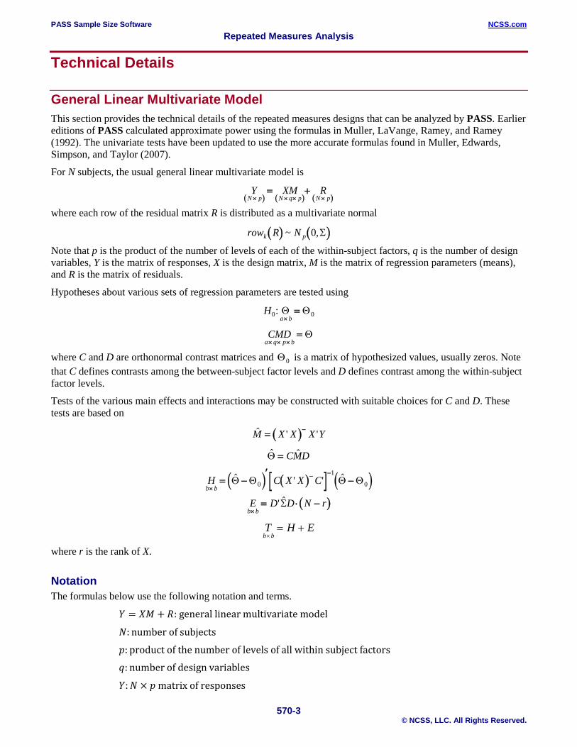
An example of a two-factor repeated measures design that can be analyzed by this procedure is shown by the following diagram.
Group 1 Group 2
Subject 1 Subject 2 Month Subject 3 Subject 4
Treatment L Treatment L 1 Treatment L Treatment L
Treatment M Treatment M 2 Treatment M Treatment M
Treatment H Treatment H 3 Treatment H Treatment H
Groups 1 and 2 form the between factor. The within factor has three levels: L, M, and H (low, medium, and high). There are four subjects in this experiment. The three treatments are applied to each subject, one per month.
This diagram shows the main features of a repeated measures design, which are
1. Each subject receives all treatments.
2. The treatments are applied through time (or space). When the treatments are applied in the same order across all subjects, it is impossible to separate treatment effects from sequence effects. Some processes that can cause sequence effects are learning, practice, or fatigue—any pattern in the responses across time that occurs without the treatment. If you think the possibility for sequence effects exists, you must make sure that the effects of prior treatments have been washed out before applying the next treatment.

PASS Sample Size Software NCSS.com Repeated Measures Analysis
570-2 © NCSS, LLC. All Rights Reserved.
3. Unlike other designs, the repeated measures design has two experimental units: between and within. In this example, the first (between) experimental unit is a subject. Subject-to-subject variability is used to test the between factor (groups). The second (within) experimental unit is the time period. In the above example, the month to month variability within a subject is used to test the treatment. The important point to realize is that the repeated measures design has two error components, the between and the within.
Assumptions The following assumptions are made when using the F test to analyze a factorial experimental design.
1. The response variable is continuous.
2. The residuals follow the normal probability distribution with mean equal to zero and constant variance.
3. The subjects are independent.
Since in a within-subject design responses coming from the same subject are not independent, assumption 3 must be modified for responses within a subject. Independence between subjects is still assumed.
4. The within-subject covariance matrices are equal for all between-subject groups. In this type of experiment, the repeated measurements on a subject may be thought of as a multivariate response vector having a certain covariance structure. This assumption states that these covariance matrices are constant from group to group.
5. When using an F test, the within-subject covariance matrices are assumed to be circular. One way of defining circularity is that the variances of differences between any two measurements within a subject are constant for all measurements. Since responses that are close together in time (or space) often have a higher correlation than those that are far apart, it is common for this assumption to be violated. This assumption is not necessary for the validity of the three multivariate tests: Wilks’ lambda, Pillai-Bartlett trace, or Hotelling-Lawley trace.
Advantages of Within-Subjects Designs Because the response to stimuli usually varies less within an individual than between individuals, the within-subject variability is usually less than (or at most equal to) the between-subject variability. By reducing the underlying variability, the same power can be achieved with a smaller number of subjects.
Disadvantages of Within-Subjects Designs 1. Practice effect. In some experiments, subjects systematically improve as they practice the task being
studies. In other cases, subjects may systematically get worse as the get fatigued or bored with the experimental task. Note that only the treatment administered first is immune to practice effects. Hence, experimenters should make an effort to balance the number of subjects receiving each treatment first.
2. Carryover effect. In many drug studies, it is important to wash out the influence of one drug completely before the next drug is administered. Otherwise, the influence of the first drug carries over into the response to the second drug.
3. Statistical analysis. The statistical model is more restrictive than in a regular factorial design since the individual responses must have certain mathematical properties.
Even in the face of all these disadvantages, repeated measures (within-subject) designs are popular in many areas of research. It is important that you recognize these problems going in so you can make sure that the design is appropriate, rather than learning of them later after the research has been conducted.
PASS Sample Size Software NCSS.com Repeated Measures Analysis
570-3 © NCSS, LLC. All Rights Reserved.
Technical Details
General Linear Multivariate Model This section provides the technical details of the repeated measures designs that can be analyzed by PASS. Earlier editions of PASS calculated approximate power using the formulas in Muller, LaVange, Ramey, and Ramey (1992). The univariate tests have been updated to use the more accurate formulas found in Muller, Edwards, Simpson, and Taylor (2007).
For N subjects, the usual general linear multivariate model is
( ) ( ) ( )Y XM R
N p N q p N p× × × ×= +
where each row of the residual matrix R is distributed as a multivariate normal
( ) ( )row R Nk p~ ,0 Σ
Note that p is the product of the number of levels of each of the within-subject factors, q is the number of design variables, Y is the matrix of responses, X is the design matrix, M is the matrix of regression parameters (means), and R is the matrix of residuals.
Hypotheses about various sets of regression parameters are tested using
Ha b0 0: Θ Θ×=
CMDa q p b× × ×
= Θ
where C and D are orthonormal contrast matrices and Θ0 is a matrix of hypothesized values, usually zeros. Note that C defines contrasts among the between-subject factor levels and D defines contrast among the within-subject factor levels.
Tests of the various main effects and interactions may be constructed with suitable choices for C and D. These tests are based on
( ) ' 'M X X X Y= −
Θ = CMD
( ) ( )[ ] ( )H C X X Cb b×
− −= −
′− ' ' Θ Θ Θ Θ0
1
0
( )E D D N rb b×
= ⋅ −' Σ
T H Eb b×
= +
where r is the rank of X.
Notation The formulas below use the following notation and terms.
𝑌𝑌 = 𝑋𝑋𝑋𝑋 + 𝑅𝑅: general linear multivariate model
𝑁𝑁: number of subjects
𝑝𝑝: product of the number of levels of all within subject factors
𝑞𝑞: number of design variables
𝑌𝑌:𝑁𝑁 × 𝑝𝑝 matrix of responses

PASS Sample Size Software NCSS.com Repeated Measures Analysis
570-4 © NCSS, LLC. All Rights Reserved.
𝑋𝑋:𝑁𝑁 × 𝑞𝑞 design matrix
𝑟𝑟 = rank(𝑋𝑋)
𝑣𝑣𝑒𝑒 = 𝑁𝑁 − 𝑟𝑟
𝑋𝑋: 𝑞𝑞 × 𝑝𝑝 matrix of regression parameters
𝑋𝑋� = (𝑋𝑋′𝑋𝑋)−𝑋𝑋′𝑌𝑌
𝑅𝑅:𝑁𝑁 × 𝑝𝑝 matrix of residuals
𝑅𝑅� = 𝑌𝑌 − 𝑋𝑋𝑋𝑋�
𝐶𝐶:𝑎𝑎 × 𝑞𝑞 fixed, known, between subject contrast matrix
𝐷𝐷: 𝑝𝑝 × 𝑏𝑏 fixed, known, within subject contrast matrix
Θ: 𝑎𝑎 × 𝑏𝑏 matrix of secondary regression parameters
Θ0: values of Θ under H0
Σ: Error covariance matrix
Σ�(𝑝𝑝 × 𝑝𝑝) =𝑅𝑅�′𝑅𝑅�𝑣𝑣𝑒𝑒
Σ∗ = 𝐷𝐷′Σ𝐷𝐷
Σ�∗ = 𝐷𝐷′Σ�𝐷𝐷
Θ = 𝐶𝐶𝑋𝑋𝐷𝐷
Θ� = 𝐶𝐶𝑋𝑋�𝐷𝐷
𝐻𝐻 = �Θ� − Θ0�′[𝐶𝐶(𝑋𝑋′𝑋𝑋)−𝐶𝐶′]−1�Θ� − Θ0�: 𝑏𝑏 × 𝑏𝑏 hypothesis sum of squares matrix
𝐸𝐸 = 𝑆𝑆𝐸𝐸 = 𝑣𝑣𝑒𝑒Σ�∗ = 𝑣𝑣𝑒𝑒𝐷𝐷′Σ�𝐷𝐷: 𝑏𝑏 × 𝑏𝑏 error sum of squares matrix
𝑇𝑇 = 𝐻𝐻 + E: 𝑏𝑏 × 𝑏𝑏 total sum of squares matrix
m = min(𝑎𝑎, 𝑏𝑏)
𝑔𝑔1(𝑣𝑣𝑒𝑒 ,𝑎𝑎, 𝑏𝑏) =[𝑣𝑣𝑒𝑒2 − 𝑣𝑣𝑒𝑒(2𝑏𝑏 + 3) + 𝑏𝑏(𝑏𝑏 + 3)](𝑎𝑎𝑏𝑏 + 2)𝑣𝑣𝑒𝑒(𝑎𝑎 + 𝑏𝑏 + 1) − (𝑎𝑎 + 2𝑏𝑏 + 𝑏𝑏2 − 1) + 4
𝑔𝑔2(𝑣𝑣𝑒𝑒 ,𝑎𝑎, 𝑏𝑏) =𝑣𝑣𝑒𝑒 + 𝑚𝑚 − 𝑏𝑏𝑣𝑣𝑒𝑒 + 𝑎𝑎
�𝑚𝑚(𝑣𝑣𝑒𝑒 + 𝑚𝑚− 𝑏𝑏)(𝑣𝑣𝑒𝑒 + 𝑎𝑎 + 2)(𝑣𝑣𝑒𝑒 + 𝑎𝑎 − 1)
𝑣𝑣𝑒𝑒(𝑣𝑣𝑒𝑒 + 𝑎𝑎 − 𝑏𝑏) − 2�
𝑔𝑔3(𝑣𝑣𝑒𝑒 ,𝑎𝑎, 𝑏𝑏) = �
𝑔𝑔4(𝑣𝑣𝑒𝑒 ,𝑎𝑎, 𝑏𝑏)
𝑔𝑔4(𝑣𝑣𝑒𝑒 ,𝑎𝑎, 𝑏𝑏)�𝑎𝑎2𝑏𝑏2 − 4𝑎𝑎2+𝑏𝑏2 − 5
if 𝑎𝑎2𝑏𝑏2 ≤ 4 if 𝑎𝑎2𝑏𝑏2 > 4
𝑔𝑔4(𝑣𝑣𝑒𝑒 ,𝑎𝑎, 𝑏𝑏) = [𝑣𝑣𝑒𝑒 − (𝑏𝑏 − 𝑎𝑎 + 1)/2] − (𝑎𝑎𝑏𝑏 − 2)/2
𝜀𝜀 = tr2(Σ∗)b tr(Σ∗2) =
�∑ 𝜆𝜆𝑘𝑘𝑏𝑏𝑘𝑘=1 �2
𝑏𝑏 ∑ 𝜆𝜆𝑘𝑘2𝑏𝑏𝑘𝑘=1
Σ∗ = 𝐷𝐷′Σ𝐷𝐷 = Υdiag(𝜆𝜆)Υ′
𝜆𝜆 = [𝜆𝜆1 𝜆𝜆2 … 𝜆𝜆𝑏𝑏]′ = vector of eigenvalues of Σ∗ Υ = [𝜐𝜐1 𝜐𝜐2 … 𝜐𝜐𝑏𝑏] = matrix of eigenvectors of Σ∗ Ω = ΔΣ∗−1

PASS Sample Size Software NCSS.com Repeated Measures Analysis
570-5 © NCSS, LLC. All Rights Reserved.
Ω𝑡𝑡 = H𝑡𝑡diag(λ)−1
ω𝑘𝑘 = υ𝑘𝑘′ H𝜐𝜐𝑘𝑘/𝜆𝜆𝑘𝑘
𝑆𝑆𝑡𝑡1 = �𝜆𝜆𝑘𝑘
𝑏𝑏
𝑘𝑘=1
𝑆𝑆𝑡𝑡2 = �𝜆𝜆𝑘𝑘
𝑏𝑏
𝑘𝑘=1
𝜔𝜔∗𝑘𝑘
𝑆𝑆𝑡𝑡3 = �𝜆𝜆𝑘𝑘2𝑏𝑏
𝑘𝑘=1
𝑆𝑆𝑡𝑡4 = �𝜆𝜆𝑘𝑘2𝑏𝑏
𝑘𝑘=1
𝜔𝜔∗𝑘𝑘
𝜆𝜆∗1 = (𝑎𝑎𝑆𝑆𝑡𝑡3 + 2𝑆𝑆𝑡𝑡4)/(𝑎𝑎𝑆𝑆𝑡𝑡1 + 2𝑆𝑆𝑡𝑡2)
𝜆𝜆∗2 = 𝑆𝑆𝑡𝑡3/𝑆𝑆𝑡𝑡1
𝑣𝑣∗1 = 𝑎𝑎𝑆𝑆𝑡𝑡1/𝜆𝜆∗1
𝑣𝑣∗2 =𝑣𝑣𝑒𝑒𝑆𝑆𝑡𝑡12
𝑆𝑆𝑡𝑡3= 𝑣𝑣𝑒𝑒𝑏𝑏𝜀𝜀
𝜔𝜔𝑢𝑢 = 𝑆𝑆𝑡𝑡2/𝜆𝜆∗1
E(𝜀𝜀̂) ≈ 𝑏𝑏−1E(𝑡𝑡1)/E(𝑡𝑡2)
E(𝜀𝜀̃) ≈ 𝑏𝑏−1[N E(𝑡𝑡1)− 2E(𝑡𝑡2)]/[𝑣𝑣𝑒𝑒 E(𝑡𝑡2) − E(𝑡𝑡1)]
E(𝑡𝑡1) = 2𝑣𝑣𝑒𝑒𝑆𝑆𝑡𝑡3 + 𝑣𝑣𝑒𝑒2𝑆𝑆𝑡𝑡12
E(𝑡𝑡2) = 𝑣𝑣𝑒𝑒(𝑣𝑣𝑒𝑒 + 2)𝑆𝑆𝑡𝑡3 + 2𝑣𝑣𝑒𝑒 � � 𝜆𝜆𝑘𝑘1𝜆𝜆𝑘𝑘2
𝑘𝑘1−1
𝑘𝑘2=1
𝑏𝑏
𝑘𝑘1=2
Table 1. Summary of the calculation of each of the statistical tests analyzed in this procedure.
Test Name Test Type Statistic df1 df2
Uncorrected F Univariate tr(𝐻𝐻)/tr(𝐸𝐸) ab 𝑣𝑣𝑒𝑒b
Geisser-Greenhouse Univariate tr(𝐻𝐻)/tr(𝐸𝐸) ab𝜀𝜀̃ 𝑣𝑣𝑒𝑒b𝜀𝜀̂
Huynh-Feldt Univariate tr(𝐻𝐻)/tr(𝐸𝐸) ab𝜀𝜀̃ 𝑣𝑣𝑒𝑒b𝜀𝜀̃
Box Univariate tr(𝐻𝐻)/tr(𝐸𝐸) a 𝑣𝑣𝑒𝑒
Hotelling-Lawley Multivariate tr(𝐻𝐻𝐸𝐸−1) ab 𝑔𝑔1(𝑣𝑣𝑒𝑒 ,𝑎𝑎, 𝑏𝑏)
Pillai-Bartlett Multivariate tr(𝐻𝐻(𝐻𝐻 + 𝐸𝐸)−1) ab
𝑔𝑔2(𝑣𝑣𝑒𝑒 ,𝑎𝑎, 𝑏𝑏)m(𝑣𝑣𝑒𝑒 + m − 𝑏𝑏)
𝑔𝑔2(𝑣𝑣𝑒𝑒 ,𝑎𝑎, 𝑏𝑏)
Wilks Multivariate |𝐸𝐸(𝐻𝐻 + 𝐸𝐸)−1| ab 𝑔𝑔3(𝑣𝑣𝑒𝑒 ,𝑎𝑎, 𝑏𝑏)

PASS Sample Size Software NCSS.com Repeated Measures Analysis
570-6 © NCSS, LLC. All Rights Reserved.
Uncorrected F Test Assuming that Σ has compound symmetry, a size α test of H0: Θ = Θ0 is given by the test statistic fu.
𝑓𝑓𝑢𝑢= tr(𝐻𝐻)/𝑎𝑎
tr(𝐸𝐸)
The critical value of this test statistic, f0(F), is based on the F distribution as follows.
𝑓𝑓0(F)=𝐹𝐹𝐹𝐹−1(1 − 𝛼𝛼; 𝑎𝑎𝑏𝑏, 𝑏𝑏𝑣𝑣𝑒𝑒 )
Using this critical value, the power is calculated as
Pr{𝑓𝑓𝑢𝑢 ≤ 𝑓𝑓0(F)}=𝐹𝐹𝐹𝐹(𝑓𝑓0(F);𝑎𝑎𝑏𝑏, 𝑏𝑏𝑣𝑣𝑒𝑒 ,𝑎𝑎𝑏𝑏𝑓𝑓𝑢𝑢)
Geisser-Greenhouse F Test The assumption that Σ has compound symmetry is usually not viable. Box (1954a,b) suggested that adjusting the degrees of freedom of the above F-ratio could compensate for the lack of compound symmetry in Σ. His adjustment has become known as the Geisser-Greenhouse adjustment.
Assuming that Σ has compound symmetry, a size α test of H0: Θ = Θ0 is given by the test statistic fu.
𝑓𝑓𝑢𝑢= tr(𝑆𝑆𝐻𝐻)/𝑎𝑎
tr(𝑆𝑆𝐸𝐸)
The expected critical value of this test statistic, f0(GG), is approximated using the F distribution as follows.
𝑓𝑓0(GG)=𝐹𝐹𝐹𝐹−1(1 − 𝛼𝛼; 𝑎𝑎𝑏𝑏E(𝜀𝜀̂), 𝑏𝑏𝑣𝑣𝑒𝑒E(𝜀𝜀̂) )
Using this critical value, the power is calculated as
Pr{𝑓𝑓𝑢𝑢 ≤ 𝑓𝑓0(GG)}≈𝐹𝐹𝐹𝐹 �𝑓𝑓0(GG)𝜆𝜆∗2𝜆𝜆∗1
𝑎𝑎𝑏𝑏𝑣𝑣∗1
𝑣𝑣∗2𝑏𝑏𝑣𝑣𝑒𝑒
;𝑣𝑣∗1, 𝑣𝑣∗2,𝜔𝜔𝑢𝑢 �
Note that the Geisser-Greenhouse adjustment is only needed for testing main effects and interactions involving within-subject factors. Main effects and interactions that involve only between-subject factors need no such adjustment.
Huynh-Feldt Test The assumption that Σ has compound symmetry is usually not viable. Box (1954a,b) suggested that adjusting the degrees of freedom of the above F-ratio could compensate for the lack of compound symmetry in Σ. His adjustment has become known as the Geisser-Greenhouse adjustment. This adjustment was further refined by Huynh and Feldt (1970), and it is popular still today.
Even if Σ does not exhibit compound symmetry, an approximate size α test of H0: Θ = Θ0 is given by the test statistic fu.
𝑓𝑓𝑢𝑢= tr(𝑆𝑆𝐻𝐻)/𝑎𝑎
tr(𝑆𝑆𝐸𝐸)
The expected critical value of this test statistic with the Huynh-Feldt adjustment, f0(HF), is approximated using the F distribution as follows.
𝑓𝑓0(HF)=𝐹𝐹𝐹𝐹−1(1 − 𝛼𝛼; 𝑎𝑎𝑏𝑏E(𝜀𝜀̃), 𝑏𝑏𝑣𝑣𝑒𝑒E(𝜀𝜀̃) )
Using this critical value, the power is calculated as
Pr{𝑓𝑓𝑢𝑢 ≤ 𝑓𝑓0(HF)}≈𝐹𝐹𝐹𝐹 �𝑓𝑓0(HF)𝜆𝜆∗2𝜆𝜆∗1
𝑎𝑎𝑏𝑏𝑣𝑣∗1
𝑣𝑣∗2𝑏𝑏𝑣𝑣𝑒𝑒
;𝑣𝑣∗1, 𝑣𝑣∗2,𝜔𝜔𝑢𝑢 �
Note that the Huynt-Feldt adjustment is only needed for testing main effects and interactions involving within-subject factors. Main effects and interactions that involve only between-subject factors need no such adjustment.

PASS Sample Size Software NCSS.com Repeated Measures Analysis
570-7 © NCSS, LLC. All Rights Reserved.
Box’s Conservative Test The assumption that Σ has compound symmetry is usually not viable. Box suggested that adjusting the degrees of freedom of the above F-ratio could compensate for the lack of compound symmetry in Σ. His adjustment has become known as the Box’s conservative adjustment.
Even if Σ does not exhibit compound symmetry, an approximate size α test of H0: Θ = Θ0 is given by the test statistic fu.
𝑓𝑓𝑢𝑢= tr(𝑆𝑆𝐻𝐻)/𝑎𝑎
tr(𝑆𝑆𝐸𝐸)
The expected critical value of this test statistic with Box’s conservative adjustment, f0(HF), is approximated using the F distribution as follows.
𝑓𝑓0(B)=𝐹𝐹𝐹𝐹−1(1− 𝛼𝛼;𝑎𝑎, 𝑣𝑣𝑒𝑒 )
Using this critical value, the power is calculated as
Pr{𝑓𝑓𝑢𝑢 ≤ 𝑓𝑓0(B)}≈𝐹𝐹𝐹𝐹 �𝑓𝑓0(B)𝜆𝜆∗2𝜆𝜆∗1
𝑎𝑎𝑏𝑏𝑣𝑣∗1
𝑣𝑣∗2𝑏𝑏𝑣𝑣𝑒𝑒
;𝑣𝑣∗1, 𝑣𝑣∗2,𝜔𝜔𝑢𝑢 �
Note that Box’s conservative adjustment is only needed for testing main effects and interactions involving within-subject factors. Main effects and interactions that involve only between-subject factors need no such adjustment.
Wilks’ Lambda Approximate F Test The hypothesis H0 0:Θ Θ= may be tested using Wilks’ likelihood ratio statistic W. This statistic is computed using
W ET= −1
An F approximation to the distribution of W is given by
( )F df
dfdf df1 2
1
21,/
/=
−ηη
where
λ = df Fdf df1 1 2,
η = −1 1W g/
df ab1=
( ) ( )[ ] ( )df g N r b a ab2 1 2 2 2= − − − + − −/ /
g a ba b
=−
+ −
2 2
2 2
124
5
PASS Sample Size Software NCSS.com Repeated Measures Analysis
570-8 © NCSS, LLC. All Rights Reserved.
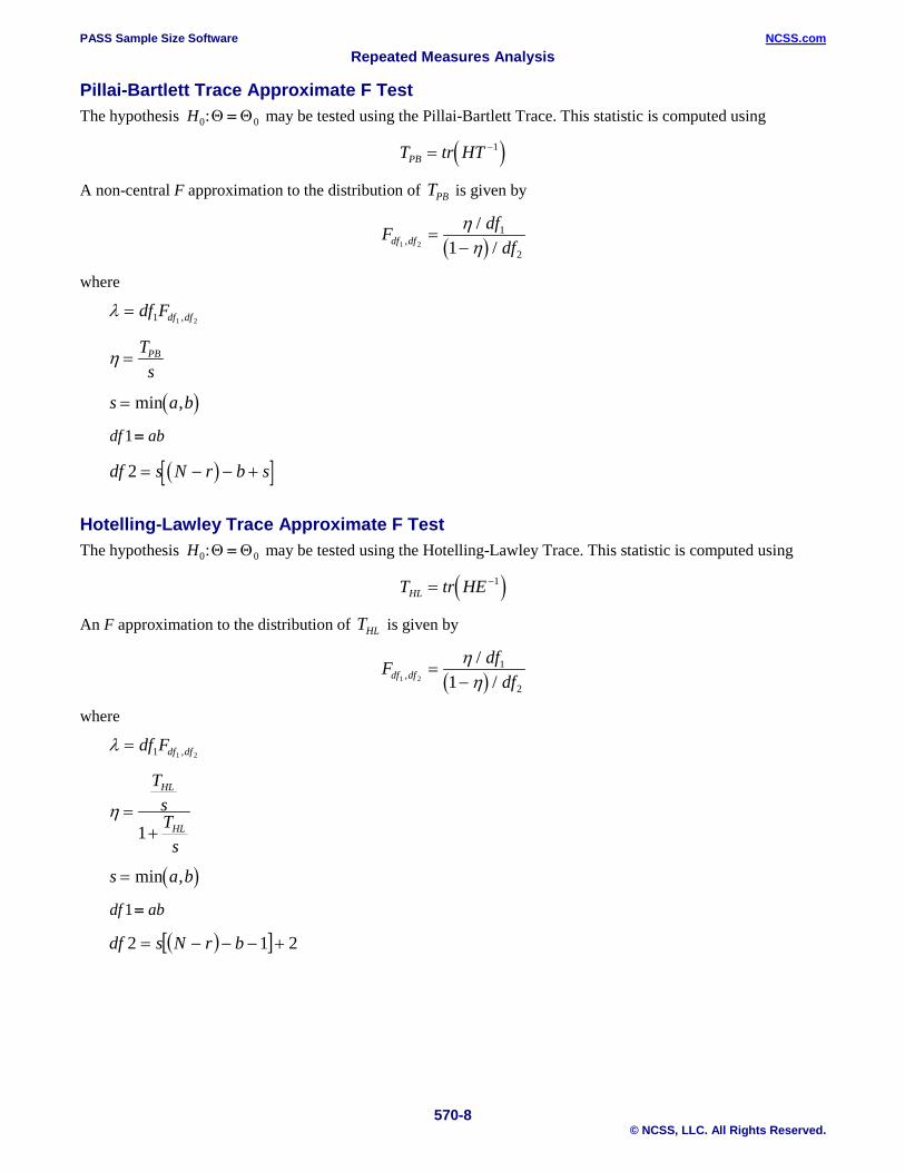
Pillai-Bartlett Trace Approximate F Test The hypothesis H0 0:Θ Θ= may be tested using the Pillai-Bartlett Trace. This statistic is computed using
( )T tr HTPB =−1
A non-central F approximation to the distribution of TPB is given by
( )F df
dfdf df1 2
1
21,/
/=
−ηη
where
λ = df Fdf df1 1 2,
η =TsPB
( )s a b= min ,
df ab1=
( )[ ]df s N r b s2 = − − +
Hotelling-Lawley Trace Approximate F Test The hypothesis H0 0:Θ Θ= may be tested using the Hotelling-Lawley Trace. This statistic is computed using
( )T tr HEHL =−1
An F approximation to the distribution of THL is given by
( )F df
dfdf df1 2
1
21,/
/=
−ηη
where
λ = df Fdf df1 1 2,
η =+
TsT
s
HL
HL1
( )s a b= min ,
df ab1=
( )[ ] 212 +−−−= brNsdf
PASS Sample Size Software NCSS.com Repeated Measures Analysis
570-9 © NCSS, LLC. All Rights Reserved.
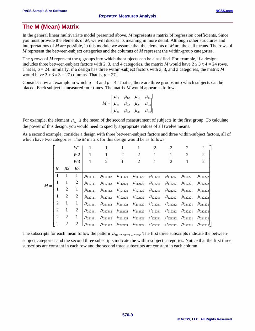
The M (Mean) Matrix In the general linear multivariate model presented above, M represents a matrix of regression coefficients. Since you must provide the elements of M, we will discuss its meaning in more detail. Although other structures and interpretations of M are possible, in this module we assume that the elements of M are the cell means. The rows of M represent the between-subject categories and the columns of M represent the within-group categories.
The q rows of M represent the q groups into which the subjects can be classified. For example, if a design includes three between-subject factors with 2, 3, and 4 categories, the matrix M would have 2 x 3 x 4 = 24 rows. That is, q = 24. Similarly, if a design has three within-subject factors with 3, 3, and 3 categories, the matrix M would have 3 x 3 x 3 = 27 columns. That is, p = 27.
Consider now an example in which q = 3 and p = 4. That is, there are three groups into which subjects can be placed. Each subject is measured four times. The matrix M would appear as follows.
M =
µ µ µ µµ µ µ µµ µ µ µ
11 12 13 14
21 22 23 24
31 32 33 34
For example, the element µ12 is the mean of the second measurement of subjects in the first group. To calculate the power of this design, you would need to specify appropriate values of all twelve means.
As a second example, consider a design with three between-subject factors and three within-subject factors, all of which have two categories. The M matrix for this design would be as follows.
M
WWW
B B B
=
1 1 1 1 1 2 2 2 22 1 1 2 2 1 1 2 23 1 2 1 2 1 2 1 2
1 2 31 1 11 1 21 2 11 2 22 1 12 1 2
111111 111112 111121 111122 111211 111212 111221 111222
112111 112112 112121 112122 112211 112212 112221 112222
121111 121112 121121 121122 121211 121212 121221 121222
122111 122112 122121 122122 122211 122212 122221 122222
211111 211112 211121 211122 211211 211212 211221 211222
212111
µ µ µ µ µ µ µ µµ µ µ µ µ µ µ µµ µ µ µ µ µ µ µµ µ µ µ µ µ µ µµ µ µ µ µ µ µ µµ µ µ µ µ µ µ µµ µ µ µ µ µ µ µµ µ µ µ µ µ µ µ
212112 212121 212122 212211 212212 212221 212222
221111 221112 221121 221122 221211 221212 221221 221222
222111 222112 222121 222122 222211 222212 222221 222222
2 2 12 2 2
The subscripts for each mean follow the pattern µB B B W W W1 2 3 1 2 3 . The first three subscripts indicate the between-subject categories and the second three subscripts indicate the within-subject categories. Notice that the first three subscripts are constant in each row and the second three subscripts are constant in each column.
PASS Sample Size Software NCSS.com Repeated Measures Analysis
570-10 © NCSS, LLC. All Rights Reserved.
Specifying the M Matrix When computing the power in a repeated measures analysis of variance, the specification of the M matrix is one of your main tasks. The program cannot do this for you. The calculated power is directly related to your choice. So your choice for the elements of M must be selected carefully and thoughtfully. When authorization and approval from a government organization is sought, you should be prepared to defend your choice of M. In this section, we will explain how you can specify M.
Before we begin, it is important that you have in mind exactly what M is. M is a table of means that represent the size of the differences among the means that you want the study or experiment to detect. That is, M gives the means under the alternative hypothesis. Under the null hypothesis, these means are assumed to be equal. Because of the complexity of the repeated measures design, it is often difficult to choose reasonable values, so PASS will help you. But it is important to remember that you are responsible for these values and that the sample sizes calculated are based on them.
One way to specify the M matrix is to do so directly into the spreadsheet. You might do this if you are calculating the ‘retrospective’ power of a study that has already been completed, or if it is simply easier to write the matrix directly. Usually, however, you will specify the M matrix in portions.
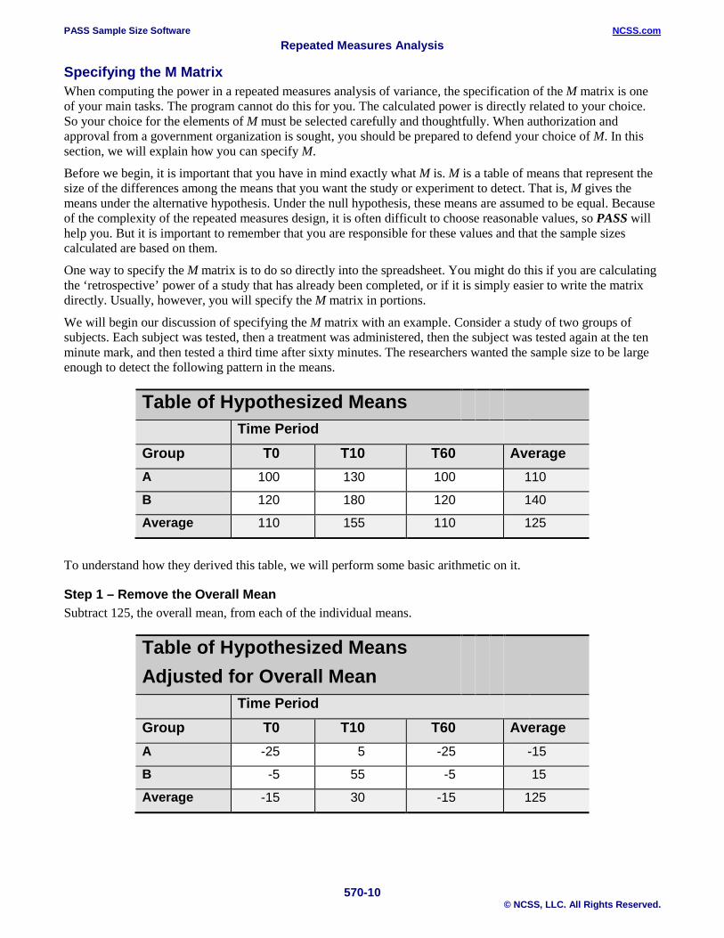
We will begin our discussion of specifying the M matrix with an example. Consider a study of two groups of subjects. Each subject was tested, then a treatment was administered, then the subject was tested again at the ten minute mark, and then tested a third time after sixty minutes. The researchers wanted the sample size to be large enough to detect the following pattern in the means.
Table of Hypothesized Means Time Period Group T0 T10 T60 Average A 100 130 100 110
B 120 180 120 140
Average 110 155 110 125
To understand how they derived this table, we will perform some basic arithmetic on it.
Step 1 – Remove the Overall Mean Subtract 125, the overall mean, from each of the individual means.
Table of Hypothesized Means Adjusted for Overall Mean
Time Period Group T0 T10 T60 Average A -25 5 -25 -15
B -5 55 -5 15
Average -15 30 -15 125
PASS Sample Size Software NCSS.com Repeated Measures Analysis
570-11 © NCSS, LLC. All Rights Reserved.
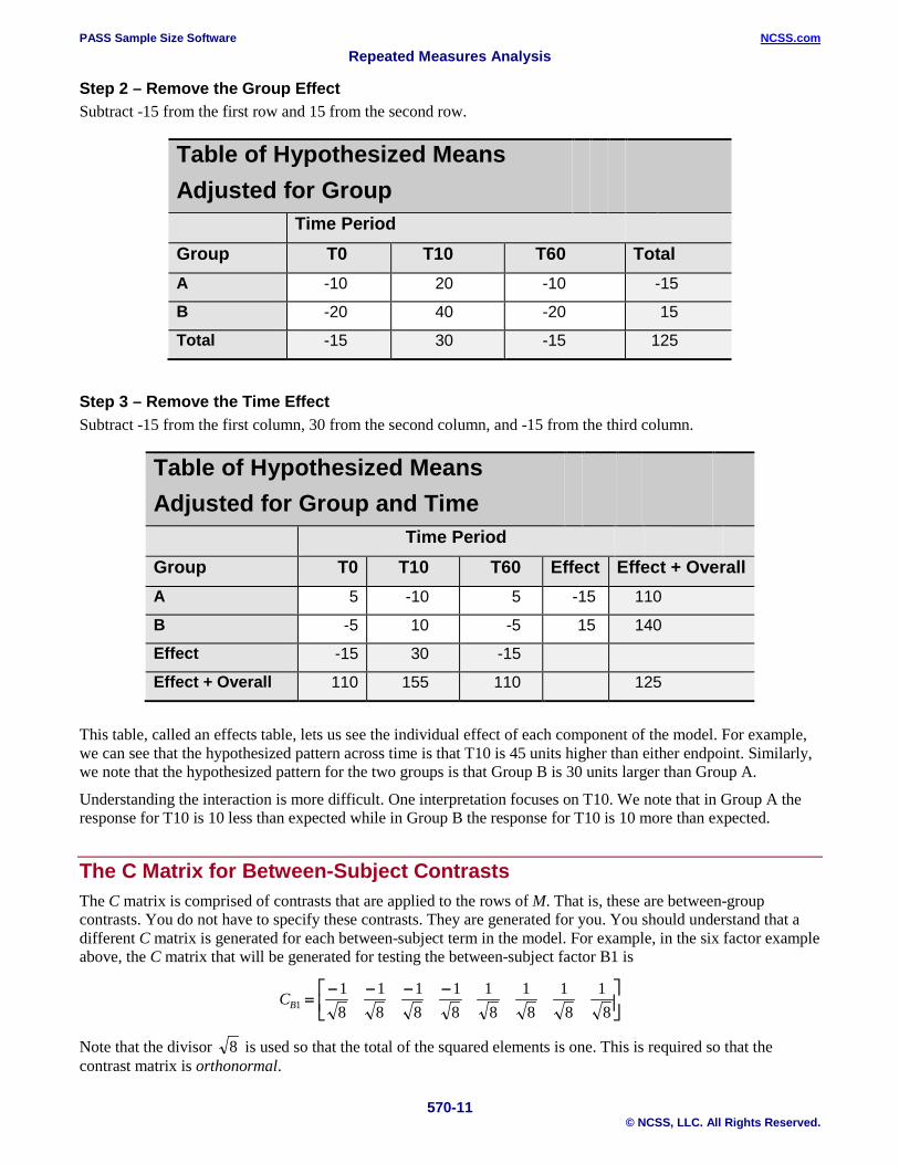
Step 2 – Remove the Group Effect Subtract -15 from the first row and 15 from the second row.
Table of Hypothesized Means Adjusted for Group
Time Period Group T0 T10 T60 Total A -10 20 -10 -15
B -20 40 -20 15
Total -15 30 -15 125
Step 3 – Remove the Time Effect Subtract -15 from the first column, 30 from the second column, and -15 from the third column.
Table of Hypothesized Means Adjusted for Group and Time
Time Period Group T0 T10 T60 Effect Effect + Overall A 5 -10 5 -15 110
B -5 10 -5 15 140
Effect -15 30 -15
Effect + Overall 110 155 110 125
This table, called an effects table, lets us see the individual effect of each component of the model. For example, we can see that the hypothesized pattern across time is that T10 is 45 units higher than either endpoint. Similarly, we note that the hypothesized pattern for the two groups is that Group B is 30 units larger than Group A.
Understanding the interaction is more difficult. One interpretation focuses on T10. We note that in Group A the response for T10 is 10 less than expected while in Group B the response for T10 is 10 more than expected.
The C Matrix for Between-Subject Contrasts The C matrix is comprised of contrasts that are applied to the rows of M. That is, these are between-group contrasts. You do not have to specify these contrasts. They are generated for you. You should understand that a different C matrix is generated for each between-subject term in the model. For example, in the six factor example above, the C matrix that will be generated for testing the between-subject factor B1 is
CB118
18
18
18
18
18
18
18
=− − − −
Note that the divisor 8 is used so that the total of the squared elements is one. This is required so that the contrast matrix is orthonormal.
PASS Sample Size Software NCSS.com Repeated Measures Analysis
570-12 © NCSS, LLC. All Rights Reserved.
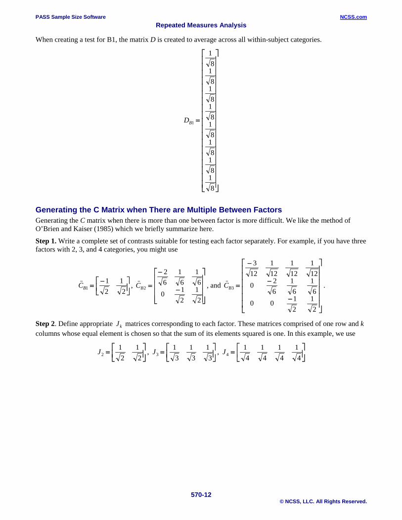
When creating a test for B1, the matrix D is created to average across all within-subject categories.
DB1
18
18
18
18
18
18
18
18
=
Generating the C Matrix when There are Multiple Between Factors Generating the C matrix when there is more than one between factor is more difficult. We like the method of O’Brien and Kaiser (1985) which we briefly summarize here.
Step 1. Write a complete set of contrasts suitable for testing each factor separately. For example, if you have three factors with 2, 3, and 4 categories, you might use
CB112
12
=−
, CB2
26
16
16
0 12
12
=
−
−
, and CB3
312
112
112
112
0 26
16
16
0 0 12
12
=
−
−
−
.
Step 2. Define appropriate Jk matrices corresponding to each factor. These matrices comprised of one row and k columns whose equal element is chosen so that the sum of its elements squared is one. In this example, we use
J212
12
=
, J3
13
13
13
=
, J4
14
14
14
14
=

PASS Sample Size Software NCSS.com Repeated Measures Analysis
570-13 © NCSS, LLC. All Rights Reserved.
Step 3. Create the appropriate contrast matrix using a direct (Kronecker) product of either the CBi matrix if the factor is included in the term or the Ji matrix when the factor is not in the term. Remember that the direct product is formed by multiplying each element of the second matrix by all members of the first matrix. Here is an example
1 23 4
1 0 10 2 01 0 3
1 2 0 0 1 23 4 0 0 3 40 0 2 4 0 00 0 6 8 0 01 2 0 0 3 63 4 0 0 9 12
⊗
−
−
=
− −− −
− −− −
As an example, we will compute the C matrix suitable for testing factor B2
C J C JB B2 2 2 4= ⊗ ⊗
Expanding the direct product results in C J C JB B2 2 2 4
12
12
26
16
16
0 12
12
14
14
14
14
212
212
112
112
112
112
0 0 14
14
14
14
14
14
14
14
248
248
148
148
148
148
248
248
148
148
148
148
2
= ⊗ ⊗
=
⊗
−
−
⊗
=
− −
− −
⊗
=
− − − − −
482
48148
148
148
148
248
248
148
148
148
148
0 0 116
116
116
116
0 0 116
116
116
116
0 0 116
116
116
116
0 0 116
116
116
116
− − −
− − − − − − − −
Similarly, the C matrix suitable for testing interaction B2B3 is
C J C CB B B B2 3 2 2 3= ⊗ ⊗
We leave the expansion of this matrix PASS, but we think you have the idea.
The D Matrix for Within-Subject Contrasts The D matrix is comprised of contrasts that are applied to the columns of M. That is, these are within-group contrasts. You do not have to specify these contrasts either. They will be generated for you. Specification of the D matrix is similar to the specification of the C matrix, except that now the matrices are all transposed.
Interactions of Between-Subject and Within-Subject Factors Interactions that include both between-subject factors and within-subject factors require that between-subject portion be specified by the C matrix and the within-subject portion be specified with the D matrix.

PASS Sample Size Software NCSS.com Repeated Measures Analysis
570-14 © NCSS, LLC. All Rights Reserved.
Covariance Matrix Assumptions The following assumptions are made when using the F test. These assumptions are not needed when using one of the three multivariate tests.
In order to use the F ratio to test hypotheses, certain assumptions are made about the distribution of the residuals eijk . Specifically, it is assumed that the residuals for each subject, e e eij ij ijT1 2, , , , are distributed as a multivariate normal with means equal to zero and covariance matrix Σ ij . Two additional assumptions are made about these covariance matrices. First, they are assumed to be equal for all subjects. That is, it is assumed that Σ Σ Σ Σ11 12= = = = Gn . Second, the covariance matrix is assumed to have a particular form called circularity. A covariance matrix is circular if there exists a matrix A such that
Σ = + +A A IT' λ
where IT is the identity matrix of order T and λ is a constant.
This property may also be defined as
σ σ σ λii jj ij+ − =2 2
One type of matrix that is circular is one that has compound symmetry. A matrix with this property has all elements on the main diagonal equal and all elements off the main diagonal equal. An example of a covariance matrix with compound symmetry is
Σ =
σ ρσ ρσ ρσρσ σ ρσ ρσρσ ρσ σ ρσ
ρσ ρσ ρσ σ
2 2 2 2
2 2 2 2
2 2 2 2
2 2 2 2
or, with actual numbers,
9 2 2 22 9 2 22 2 9 22 2 2 9
An example of a matrix which does not have compound symmetry but is still circular is
1 1 1 12 2 2 23 3 3 34 4 4 4
1 2 3 41 2 3 41 2 3 41 2 3 4
2 0 0 00 2 0 00 0 2 00 0 0 2
4 3 4 53 6 5 64 5 8 75 6 7 10
+
+
=
Needless to say, the need to have the covariance matrix circular is a very restrictive assumption.
PASS Sample Size Software NCSS.com Repeated Measures Analysis
570-15 © NCSS, LLC. All Rights Reserved.
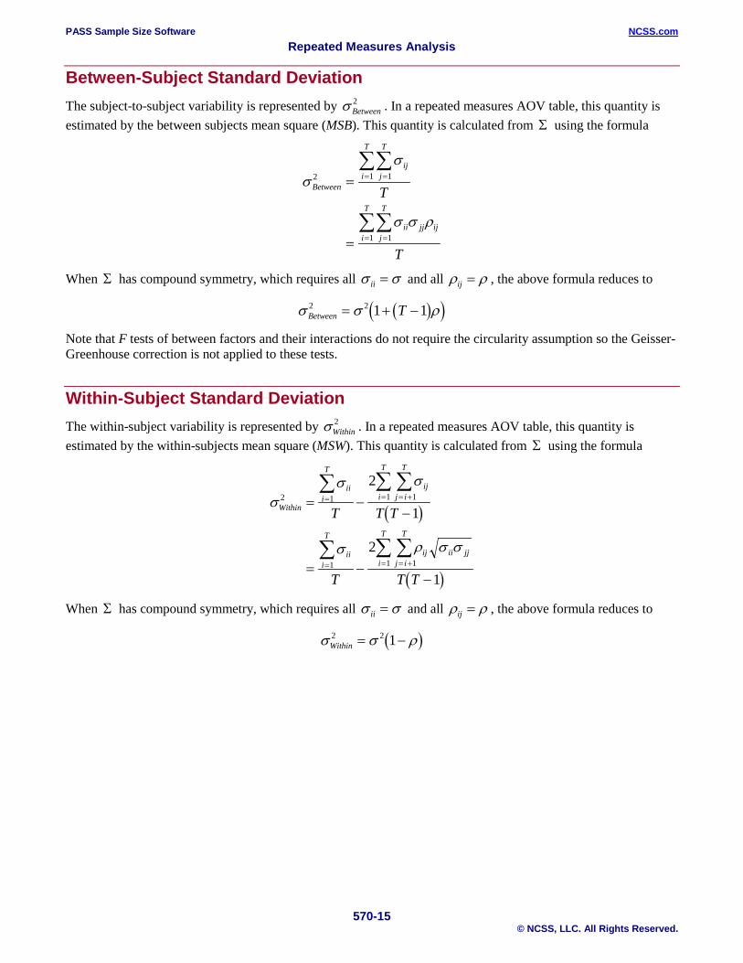
Between-Subject Standard Deviation The subject-to-subject variability is represented by σ Between
2 . In a repeated measures AOV table, this quantity is estimated by the between subjects mean square (MSB). This quantity is calculated from Σ using the formula
σσ
σ σ ρ
Between
ijj
T
i
T
ii jj ijj
T
i
TT
T
2 11
11
=
=
==
==
∑∑
∑∑
When Σ has compound symmetry, which requires all σ σii = and all ρ ρij = , the above formula reduces to
( )( )σ σ ρBetween T2 2 1 1= + −
Note that F tests of between factors and their interactions do not require the circularity assumption so the Geisser-Greenhouse correction is not applied to these tests.
Within-Subject Standard Deviation The within-subject variability is represented by σWithin
2 . In a repeated measures AOV table, this quantity is estimated by the within-subjects mean square (MSW). This quantity is calculated from Σ using the formula
( )
( )
σσ σ
σ ρ σ σ
Within
iii
T
ijj i
T
i
T
iii
T
ij ii jjj i
T
i
T
T T T
T T T
2 1 11
1 11
2
1
2
1
= −−
= −−
= = +=
= = +=
∑ ∑∑
∑ ∑∑
When Σ has compound symmetry, which requires all σ σii = and all ρ ρij = , the above formula reduces to
( )σ σ ρWithin2 2 1= −

PASS Sample Size Software NCSS.com Repeated Measures Analysis
570-16 © NCSS, LLC. All Rights Reserved.
Estimating Sigma and Rho from Existing Data Using the above results for existing data, approximate values for σ and ρ may be estimated from a previous analysis of variance table that provides estimates of MSB and MSW. Solving the above equations for σ and ρ yields
( )ρ σ σ
σ σ=
−+ −
Between Within
Between WithinT
2 2
2 21
σ σρ
22
1=
−Within
Substituting MSB for σ Between2 and MSW for σWithin
2 yields the estimates
( )ρ = −
+ −MSB MSW
MSB T MSW1
σρ
2
1=
−MSW
Note that these estimators assume that the design meets the circularity assumption, which is usually not the case. However, they provide crude estimates that can be used in planning.
Procedure Options This section describes the options that are unique to this procedure. To find out more about using the other tabs, go to the Procedure Window chapter.
Design: Means Tab The Design: Means tab contains options for the test type, alpha and power, number and type of factors, means, and sample size.
Solve For
Solve For This option specifies whether you want to solve for power or sample size. This choice controls which options are displayed in the Sample Size section. Note that no plots are generated when you solve for n.
If you select sample size, two more options appear.
Solve For Sample Size ‘Based On’ Specify which test statistic you want to use when solving for a sample size.
Note that the regular F-Test can only be used with a constant variance and single autocorrelation value.
Solve For Sample Size Using ‘Term’ Specify which term to use when searching for a sample size. The power of this term’s test will be evaluated as the search is conducted.
All If you want to use all terms, select ‘All.’

PASS Sample Size Software NCSS.com Repeated Measures Analysis
570-17 © NCSS, LLC. All Rights Reserved.
Note Only terms that are active may be selected. If you select a term that is not active, you will be prompted to select another term.
Power and Alpha
Minimum Power Per Term Enter a value for the minimum power to be achieved when solving for the sample size. The resulting sample size is large enough so that the power is greater than this amount. This search is conducted using either all terms, or only a specific term.
Power is the probability of rejecting the null hypothesis when it is false. Beta, the probability of obtaining a false negative on the statistical test, is equal to 1-power, so specifying power implicitly specifies beta.
Range Since power is a probability, its valid range is between 0 and 1.
Recommended Different disciplines have different standards for power. A popular value is 0.9, but 0.8 is also popular.
Alpha for All Terms Enter a single value for the alpha to be used in all statistical tests.
Alpha is the probability of obtaining a false positive on a statistical test. That is, it is the probability of rejecting a true null hypothesis. The null hypothesis is usually that the variance of the means (or effects is) zero.
Range Since Alpha is a probability, it is bounded by 0 and 1. Commonly, it is between 0.001 and 0.250.
Recommended Alpha is usually set to 0.05 for two-sided tests such as those considered here.
Design and Effects
Number of Factors Select the number of between and within factors included in the design. Up to three between and within factors may be selected.
Between Factors Between factors are variables that separate subjects into groups. Examples of between factors are location, gender, and age group.
Within Factors Within (subject) factors are variables whose levels all occur on a single subject. Examples of within factors are time, dose (when a subject receives all doses), and location on a subject.
Mean Input Type The detectable difference among the means (or effects) of a term is calculated from the appropriate set of means (or effects). Indicate whether you will enter the means separately for each term or directly as a single matrix the combines the means for all terms.
PASS Sample Size Software NCSS.com Repeated Measures Analysis
570-18 © NCSS, LLC. All Rights Reserved.
Means, Interaction Effects Enter the mean (or effects) separately for each term.
Means Matrix in Spreadsheet Enter a set of means directly into the spreadsheet. The individual effects for each term will be calculated from this matrix.
Design and Effects – Levels and Means
Levels Specify the number of levels (categories) for each factor. Typical values are from 2 to 8.
Means This option appears if Mean Input Type is set to ‘Means, Interaction Effects.’ Select the method used to enter the means. Since only σm (the standard deviation calculated from these means) is used, the value of σm can be entered directly. There are two ways in which you can enter this value.
Enter the values in the box to the right.
As a Std Dev Enter value of σm directly to the right. The value entered represents the magnitude of the variation among the effects of this term that you want to detect.
You can use the Standard Deviation Estimator window to calculate the value of σm for various sets of means. This window is obtained by pressing the ‘Sm’ icon to the right.
List of Means Enter a list of means directly to the right. The value of σm is calculated from these means.
Columns Containing the Means This option appears if Mean Input Type is set to ‘Means, Interaction Effects.’ Use this option to the specify spreadsheet columns containing a hypothesized matrix of mean from which the value of σm can be computed for each term. To select the spreadsheet columns and enter the means into the spreadsheet, press the icon directly to the right.
In the spreadsheet, the between factors are represented across the columns and the within factors are represented down the rows.
The number of columns specified must equal the number of groups. The number of groups is equal to the product of the number of levels of the between factors. If no between factors are specified, the number of groups is one.
The number of rows with data in these columns must equal the number of times a subject is measured. Thus the number of rows is equal to the product of the number of levels of the within factors. If no within factors are specified, the number of rows is one.
For example, suppose you are designing an experiment that is to have two between factors (A & B) and two within factors (D & E), each with two levels. The four columns of the spreadsheet would be
A1B1 A1B2 A2B1 A2B2
PASS Sample Size Software NCSS.com Repeated Measures Analysis
570-19 © NCSS, LLC. All Rights Reserved.
The rows of the spreadsheet would represent
D1E1
D1E2
D2E1 D2E2
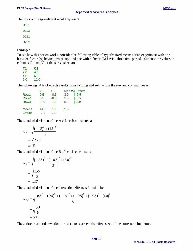
Example To see how this option works, consider the following table of hypothesized means for an experiment with one between factor (A) having two groups and one within factor (B) having three time periods. Suppose the values in columns C1 and C2 of the spreadsheet are
C1 C2 2.0 4.0 4.0 6.0 6.0 11.0
The following table of effects results from forming and subtracting the row and column means. C1 C2 | Means | Effects
Row1 0.5 -0.5 | 3.0 | -2.5 Row2 0.5 -0.5 | 5.0 | -0.5 Row3 -1.0 1.0 | 8.5 | 3.0
--- --- | --- Means 4.0 7.0 | 5.5 Effects -1.5 1.5
The standard deviation of the A effects is calculated as
( ) ( )σ A =− +
==
15 152
2 2515
2 2. .
..
The standard deviation of the B effects is calculated as
( ) ( ) ( )σ B =− + − +
=
=
2 5 0 5 303
1553
2 27
2 2 2. . .
.
. The standard deviation of the interaction effects is found to be
( ) ( ) ( ) ( ) ( ) ( )σ AB =+ + − + − + − +
=
=
0 5 0 5 10 0 5 0 5 106
306
0 71
2 2 2 2 2 2. . . . . .
.
. These three standard deviations are used to represent the effect sizes of the corresponding terms.

PASS Sample Size Software NCSS.com Repeated Measures Analysis
570-20 © NCSS, LLC. All Rights Reserved.
K (Mean Multipliers) It is often useful to conduct a sensitivity analysis to determine the relationship between the means and the power or sample size. Instead of having to enter all values of the means over and over, this option allows you to enter multipliers that will be applied to the σm’s of each term. A separate power calculation or sample size search is generated for each value of K. These values become the horizontal axis in the second power chart. For example, if a σm is 80, setting this option to ‘0.5 1 1.5’ would result in three σm values: 40, 80, and 120.
If you want to ignore this setting, enter ‘1’.
Sample Size (when ‘Solve For’ = Power) The options available for sample size depend on the setting of Solve For. This section is for when you have set Solve For to Power.
Group Allocation Specify how subjects are allocated to groups.
Equal (n1 = n2 = … = n) The sample size of every group is n. That is, all group sample sizes are equal. The values of n are entered in the box below.
Unequal (Enter n1, n2, … Individually) The sample sizes of each group are possibly different and are entered individually as a list below.
n (Size Per Group, Equal Group Size) Enter n, the number of subjects in each group. Sample sizes must be 2 or more.
You can specify a single value or a list. Enter a single value to be used as the sample size of all groups. If you enter a list of values, a separate power analysis is calculated for each value in the list.
n1, n2, … (List) Enter a list of group sample sizes, one per group. The number of groups is equal to the product of the between factor levels. The number of items entered must be equal to the number of groups. If not enough values are entered, the last value is used for remaining groups.
Group Order The items in the list correspond to the treatment combinations of the between factors. The order of the groups is such that the last factor changes the fastest and the first changes the slowest. Here are some examples of how the groups are numbered.
One Between Factor If there is one between factor ‘A’ with five levels, group 1 corresponds to A1, group 2 to A2, and so on.
Two Between Factors If there are two between factors ‘A’ and ‘B’ each with two levels, the groups are assigned as follows:
Group Level 1 A1B1 2 A1B2 3 A2B1 4 A2B2

PASS Sample Size Software NCSS.com Repeated Measures Analysis
570-21 © NCSS, LLC. All Rights Reserved.
Three Between Factors If there are three between factors ‘A,’ ‘B,’ and ‘C’ each with two levels, the groups are assigned as follows:
Group Level 1 A1B1C1 2 A1B1C2 3 A1B2C1 4 A1B2C2 5 A2B1C1 6 A2B1C2 7 A2B2C1 8 A2B2C2
Sample Size (when ‘Solve For’ = Sample Size) The options available for sample size depend on the setting of Solve For. This section is for when you have set Solve For to Sample Size.
Group Allocation Specify how subjects are allocated to groups during the sample size search.
Equal (n1 = n2 = …) The search is conducted with all group sample sizes are equal.
Unequal The search is conducted using the Allocation Pattern given below. This pattern gives the ratio of each sample size to the smallest (or the proportion of the total sample size in each group).
Allocation Pattern Enter a list of positive numbers, one per group, that represent the relative sample size of each group. This pattern will be used (within rounding) as the sample size search is conducted. Only the relative magnitudes of the values matter when specifying the pattern.
The number of groups is equal to the product of the between factor levels. The number of items entered must be equal to the number of groups. If not enough values are entered, the last value is used for remaining groups.
The numbers in the pattern may be interpreted in different ways:
Proportions Enter the proportions of all subjects in each group. For example, suppose you have one between factor with four levels in which twice as many subjects are desired in the second group as in the other groups.
You might enter: 0.2 0.4 0.2 0.2
Which means: 20% in the first, third, and four groups and 40% in the second.
Ratios Enter the ratio of each group to the smallest value. For example, suppose you have one between factor with four levels in which twice as many subjects are desired in the second group.
You might enter:1 2 1 1
Which means: 20% in the first, third, and four groups and 40% in the second.

PASS Sample Size Software NCSS.com Repeated Measures Analysis
570-22 © NCSS, LLC. All Rights Reserved.
Group Order The items in the list correspond to the treatment combinations of the between factors. The order of the groups is such that the last factor changes the fastest and the first changes the slowest. Here are some examples of how the groups are numbered.
One Between Factor If there is one between factor ‘A’ with five levels, group 1 corresponds to A1, group 2 to A2, and so on.
Two Between Factors If there are two between factors ‘A’ and ‘B’ each with two levels, the groups are assigned as follows:
Group Level 1 A1B1 2 A1B2 3 A2B1 4 A2B2
Three Between Factors If there are three between factors ‘A,’ ‘B,’ and ‘C’ each with two levels, the groups are assigned as follows:
Group Level 1 A1B1C1 2 A1B1C2 3 A1B2C1 4 A1B2C2 5 A2B1C1 6 A2B1C2 7 A2B2C1 8 A2B2C2
Interactions Tab Enter the effects of all interactions in your design.
Effects of Interaction Terms
Enter Effects As Select the method used to enter the effects. Since only the standard deviation of the effects (σm) is needed, only this value is entered. There are two ways in which you can enter this value.
Standard Deviation Enter the value of σm directly. The Sm button to the right will help you calculate an appropriate value.
Multiple of Another Term Enter the value of σm as a multiple of another term. This option is useful when you are not particularly interested in this term, but you do want to use a reasonable value.
For example, suppose σm for B1 is 4.73 and you want the σm for this term to be twice that. You would enter ‘2.0’ as the multiplier and select ‘B1’ as the term.
PASS Sample Size Software NCSS.com Repeated Measures Analysis
570-23 © NCSS, LLC. All Rights Reserved.
Standard Deviation Enter a single value for σm. This value represents the magnitude of the differences among the effects that is to be detected. By ‘detected,’ we mean that if σm is this large, the null hypothesis of effect equality will likely be rejected.
Multiplier Calculate this term's σm as this multiplier times the σm of another term. The multiplier must be greater than zero.
The formula is
σm(This Term) = multiplier x σm(Other Term)
Term Select the term used as the other term. The value of σm is calculated using the formula
σm(This Term) = multiplier x σm(Other Term)
Note that the term selected here MUST be active in this analysis.
Variances Tab This tab specifies the variance-covariance matrix of the within factors.
Variance-Covariance Matrix
Input Type Specify the method used to define the variance-covariance matrix.
Constant σ and ρ Specify a constant standard deviation and autocorrelation from which the variance-covariance matrix is constructed. This option must be used when you want results for the univariate F-test.
Non-Constant σ's and ρ's This option generates a variance-covariance matrix based on the settings for the standard deviations (σ's) and the autocorrelations.
Variance-Covariance Matrix in Spreadsheet The variance-covariance matrix is read in from the columns of the spreadsheet. This is the most flexible method, but specifying a variance-covariance matrix is tedious. You will usually only use this method when a specific covariance is given to you.
Non-Constant σ's and ρ's in Spreadsheet The variance-covariance matrix is read in from the columns of the spreadsheet. The σ's are on the diagonal and the ρ's are on the off-diagonal.
Note that the spreadsheet is shown by selecting the menus: "Window" and then "Spreadsheet", or by pressing the spreadsheet icon at the right.
PASS Sample Size Software NCSS.com Repeated Measures Analysis
570-24 © NCSS, LLC. All Rights Reserved.
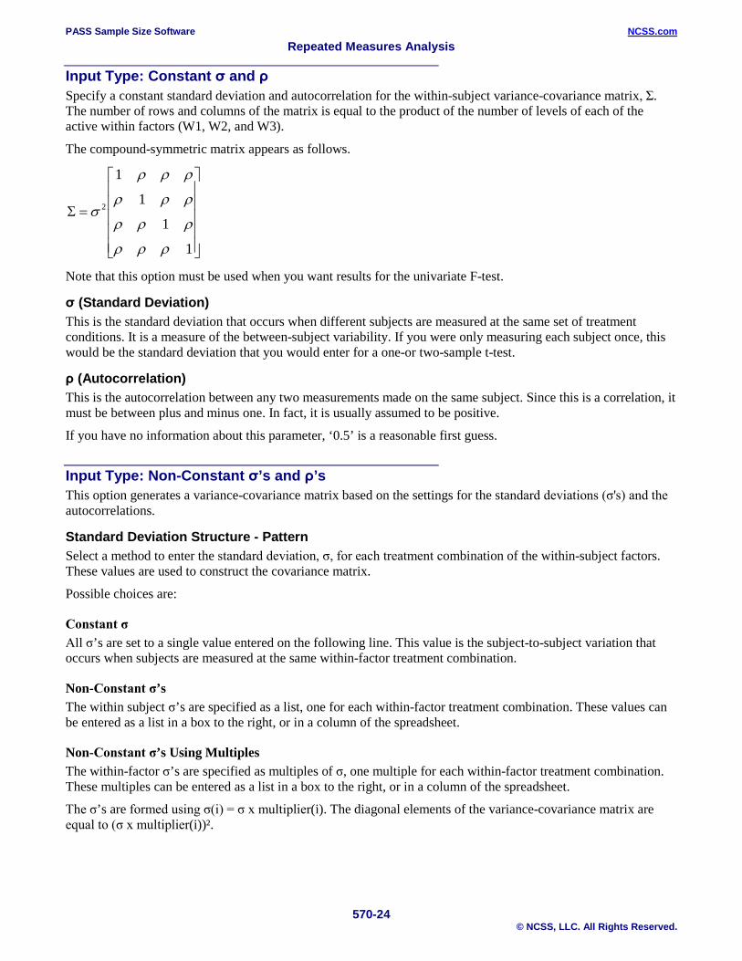
Input Type: Constant σ and ρ Specify a constant standard deviation and autocorrelation for the within-subject variance-covariance matrix, Σ. The number of rows and columns of the matrix is equal to the product of the number of levels of each of the active within factors (W1, W2, and W3).
The compound-symmetric matrix appears as follows.
=Σ
1
1
1
1
2
ρρρ
ρρρ
ρρρ
ρρρ
σ
Note that this option must be used when you want results for the univariate F-test.
σ (Standard Deviation) This is the standard deviation that occurs when different subjects are measured at the same set of treatment conditions. It is a measure of the between-subject variability. If you were only measuring each subject once, this would be the standard deviation that you would enter for a one-or two-sample t-test.
ρ (Autocorrelation) This is the autocorrelation between any two measurements made on the same subject. Since this is a correlation, it must be between plus and minus one. In fact, it is usually assumed to be positive.
If you have no information about this parameter, ‘0.5’ is a reasonable first guess.
Input Type: Non-Constant σ’s and ρ’s This option generates a variance-covariance matrix based on the settings for the standard deviations (σ's) and the autocorrelations.
Standard Deviation Structure - Pattern Select a method to enter the standard deviation, σ, for each treatment combination of the within-subject factors. These values are used to construct the covariance matrix.
Possible choices are:
Constant σ All σ’s are set to a single value entered on the following line. This value is the subject-to-subject variation that occurs when subjects are measured at the same within-factor treatment combination.
Non-Constant σ’s The within subject σ’s are specified as a list, one for each within-factor treatment combination. These values can be entered as a list in a box to the right, or in a column of the spreadsheet.
Non-Constant σ’s Using Multiples The within-factor σ’s are specified as multiples of σ, one multiple for each within-factor treatment combination. These multiples can be entered as a list in a box to the right, or in a column of the spreadsheet.
The σ’s are formed using σ(i) = σ x multiplier(i). The diagonal elements of the variance-covariance matrix are equal to (σ x multiplier(i))².

PASS Sample Size Software NCSS.com Repeated Measures Analysis
570-25 © NCSS, LLC. All Rights Reserved.
Autocorrelation Structure Specify the autocorrelation structure of the matrix associated with each factor. The number of diagonal elements in the matrix is equal to the number of levels in the factor. The final autocorrelation matrix is the Kronecker product of these individual factor autocorrelation matrices. This method was presented in Naik and Rao (2001).
For example, suppose an experiment is being designed with two within factors: 1) three equal-space time points and 2) two locations in the brain. Suppose that an AR(1) pattern is assumed for the time factor with autocorrelation γ = 0.6 and a constant pattern is assumed for the location factor with autocorrelation θ = 0.1. The individual factor autocorrelation matrices would be
=
=
16.036.0
6.016.0
36.06.01
1
1
1
2
2
γγ
γγ
γγ
A ,
=
=
11.0
1.01
1
1
θ
θB
And the final autocorrelation structure would be
=
=⊗
1100.0600.0060.0360.0036.0
100.01060.0600.0036.0360.0
600.0060.01100.0600.0060.0
060.0600.0100.01060.0600.0
360.0036.0600.0060.01100.0
036.0360.0060.0600.0100.01
1
1
1
1
1
1
22
22
22
22
θγγθγθγ
θγθγθγγ
γγθθγγθ
γθγθγθγ
γθγγγθθ
θγγγθγθ
BA
We will now present the various options available for quickly specifying the autocorrelation structure of an individual factor.
Constant A single value of ρ is used as the autocorrelation for all off-diagonal elements of the matrix. This matrix pattern is called compound symmetry.
The matrix appears as follows.
1
1
1
1
ρρρ
ρρρ
ρρρ
ρρρ

PASS Sample Size Software NCSS.com Repeated Measures Analysis
570-26 © NCSS, LLC. All Rights Reserved.
AR(1) A single value of ρ is used to generate a first order autocorrelation pattern. This pattern reduces the autocorrelation at each successive step by multiplying the value at the last step by ρ. The times (or locations) are assumed to be equi-spaced.
The matrix appears as follows.
1
1
1
1
23
2
32
ρρρ
ρρρ
ρρρ
ρρρ
LEAR A single value of ρ and a dampening value δ are used to generate the autocorrelations using the LEAR (linear exponent autoregressive) correlation structure proposed by Simpson, Edwards, Muller, Sen, and Styner (2010). The times (or locations) need to be specified. The formula for this structure is
−−
+=minmax
minminwhere,
dddd
dA jkA δρ
where kjjk ttd −= , tj and tk are any two measurement points (times or locations), dmin is the minimum djk, dmax is the maximum djk, and δ is a dampening constant.
The t’s often are entered as increasing integers, such as 1, 2, 3, and so on. But this is not necessary. The only required characteristic is that they be strictly increasing. The authors recommend that the t’s be scaled so that dmin
= 1.
Banded A list of correlation values ρ1, ρ2, ... is used to create a banded correlation matrix. If note enough values are entered, the last entered value is carried forward.
A banded correlation matrix for a factor with six levels looks as follows.
1
1
1
1
1
1
12345
11234
21123
32112
43211
54321
ρρρρρ
ρρρρρ
ρρρρρ
ρρρρρ
ρρρρρ
ρρρρρ
PASS Sample Size Software NCSS.com Repeated Measures Analysis
570-27 © NCSS, LLC. All Rights Reserved.
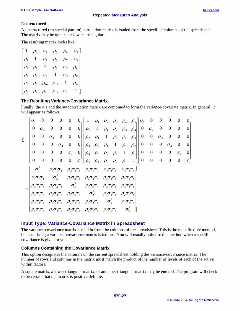
Unstructured A unstructured (no special pattern) correlation matrix is loaded from the specified columns of the spreadsheet. The matrix may be upper-, or lower-, triangular.
The resulting matrix looks like
1
1
1
1
1
1
14131185
14121074
1312963
1110952
87651
54321
ρρρρρ
ρρρρρ
ρρρρρ
ρρρρρ
ρρρρρ
ρρρρρ
The Resulting Variance-Covariance Matrix Finally, the σ’s and the autocorrelation matrix are combined to form the variance-covariate matrix. In general, it will appear as follows.
=
=Σ
26651642633624615
65125541532523514
64254124431422413
63353243123321312
62452342232122211
61551441331221121
6
5
4
3
2
1
12345
11234
21123
32112
43211
54321
6
5
4
3
2
1
00000
00000
00000
00000
00000
00000
1
1
1
1
1
1
00000
00000
00000
00000
00000
00000
σσσρσσρσσρσσρσσρ
σσρσσσρσσρσσρσσρ
σσρσσρσσσρσσρσσρ
σσρσσρσσρσσσρσσρ
σσρσσρσσρσσρσσσρ
σσρσσρσσρσσρσσρσ
σ
σ
σ
σ
σ
σ
ρρρρρ
ρρρρρ
ρρρρρ
ρρρρρ
ρρρρρ
ρρρρρ
σ
σ
σ
σ
σ
σ
Input Type: Variance-Covariance Matrix in Spreadsheet The variance-covariance matrix is read in from the columns of the spreadsheet. This is the most flexible method, but specifying a variance-covariance matrix is tedious. You will usually only use this method when a specific covariance is given to you.
Columns Containing the Covariance Matrix This option designates the columns on the current spreadsheet holding the variance-covariance matrix. The number of rows and columns in the matrix must match the product of the number of levels of each of the active within factors.
A square matrix, a lower triangular matrix, or an upper triangular matrix may be entered. The program will check to be certain that the matrix is positive definite.
PASS Sample Size Software NCSS.com Repeated Measures Analysis
570-28 © NCSS, LLC. All Rights Reserved.
The columns of the spreadsheet must be ordered so that the subscripts of the first within factor vary the slowest. For example, if you had three within factors, each at two levels, the subscripts of eight columns of the spreadsheet would be 111, 112, 121, 122, 211, 212, 221, and 222. Here, ‘121’ means that W1 is at its first level, W2 is at its second level, and W3 is at its first level.
Input Type: Non-Constant σ’s and ρ’s in Spreadsheet This option designates the columns on the current spreadsheet holding the σ’s and ρ’s. The σ’s are entered on the diagonal. The ρ’s are entered on the off-diagonal.
The number of rows and columns in the matrix must match the product of the number of levels of each of the active within factors.
A square matrix, a lower triangular matrix, or an upper triangular matrix may be entered. The program will check to be certain that the resulting covariance matrix is positive definite.
The columns of the spreadsheet must be ordered so that the subscripts of the first within factor vary the slowest. For example, if you had three within factors, each at two levels, the subscripts of eight columns of the spreadsheet would be 111, 112, 121, 122, 211, 212, 221, and 222. Here, ‘121’ means that W1 is at its first level, W2 is at its second level, and W3 is at its first level.
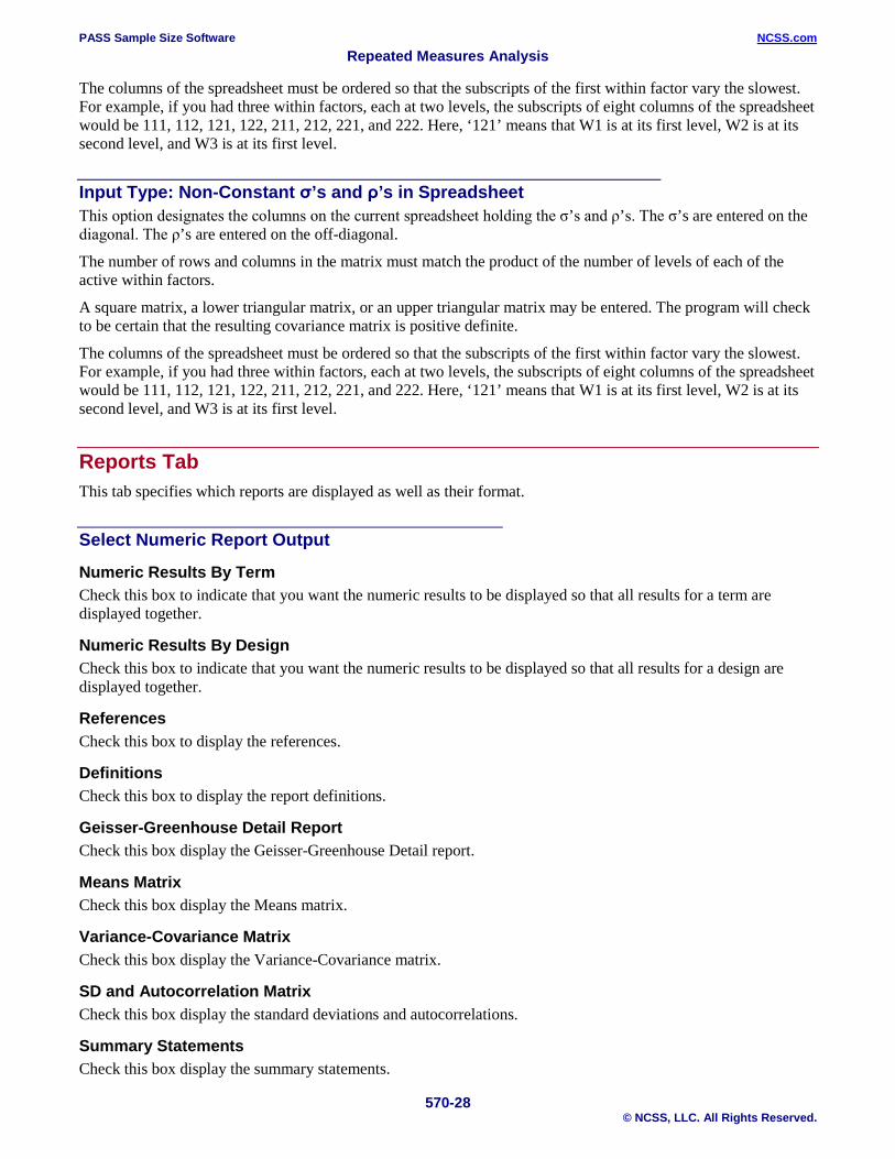
Reports Tab This tab specifies which reports are displayed as well as their format.
Select Numeric Report Output
Numeric Results By Term Check this box to indicate that you want the numeric results to be displayed so that all results for a term are displayed together.
Numeric Results By Design Check this box to indicate that you want the numeric results to be displayed so that all results for a design are displayed together.
References Check this box to display the references.
Definitions Check this box to display the report definitions.
Geisser-Greenhouse Detail Report Check this box display the Geisser-Greenhouse Detail report.
Means Matrix Check this box display the Means matrix.
Variance-Covariance Matrix Check this box display the Variance-Covariance matrix.
SD and Autocorrelation Matrix Check this box display the standard deviations and autocorrelations.
Summary Statements Check this box display the summary statements.

PASS Sample Size Software NCSS.com Repeated Measures Analysis
570-29 © NCSS, LLC. All Rights Reserved.
Test Statistic Indicate the test that is to be used in the Summary Statements.
Maximum Order of Terms on Reports Indicate the maximum order of terms to be reported on. Often, higher-order interactions are of little interest and so they may be omitted. For example, enter a ‘2’ here to limit output to individual factors and two-way interactions.
Skip to Next Row After The names of the terms can be too long to fit in the space provided. If the name contains more characters than this, the rest of the output is placed on a separate line. Enter ‘1’ when you want every term’s results printed on two lines. Enter ‘100’ when you want every variable’s results printed on one line.
Decimal Places for Numeric Reports Specify the number of decimal places in the reports for each item.
Factor Labels Specify a label for each factor. The label can consist of several letters. When several letters are used, the labels for the interactions may be long and confusing. Of course, you must be careful not to use the same label for two factors.
One of the easiest sets of labels is to use A, B, and C for the between factors and D, E, and F for the within factors. A useful alternative is to use B1, B2, and B3 for the between factors and W1, W2, and W3 for the within factors.
PASS Sample Size Software NCSS.com Repeated Measures Analysis
570-30 © NCSS, LLC. All Rights Reserved.
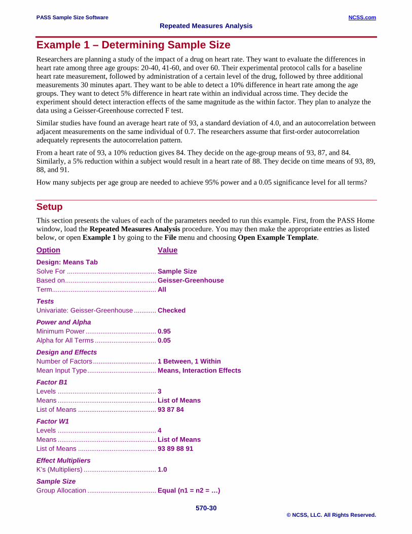
Example 1 – Determining Sample Size Researchers are planning a study of the impact of a drug on heart rate. They want to evaluate the differences in heart rate among three age groups: 20-40, 41-60, and over 60. Their experimental protocol calls for a baseline heart rate measurement, followed by administration of a certain level of the drug, followed by three additional measurements 30 minutes apart. They want to be able to detect a 10% difference in heart rate among the age groups. They want to detect 5% difference in heart rate within an individual across time. They decide the experiment should detect interaction effects of the same magnitude as the within factor. They plan to analyze the data using a Geisser-Greenhouse corrected F test.
Similar studies have found an average heart rate of 93, a standard deviation of 4.0, and an autocorrelation between adjacent measurements on the same individual of 0.7. The researchers assume that first-order autocorrelation adequately represents the autocorrelation pattern.
From a heart rate of 93, a 10% reduction gives 84. They decide on the age-group means of 93, 87, and 84. Similarly, a 5% reduction within a subject would result in a heart rate of 88. They decide on time means of 93, 89, 88, and 91.
How many subjects per age group are needed to achieve 95% power and a 0.05 significance level for all terms?
Setup This section presents the values of each of the parameters needed to run this example. First, from the PASS Home window, load the Repeated Measures Analysis procedure. You may then make the appropriate entries as listed below, or open Example 1 by going to the File menu and choosing Open Example Template.
Option Value Design: Means Tab Solve For ................................................ Sample Size Based on ................................................. Geisser-Greenhouse Term........................................................ All Tests Univariate: Geisser-Greenhouse ............ Checked
Power and Alpha Minimum Power ...................................... 0.95 Alpha for All Terms ................................. 0.05
Design and Effects Number of Factors .................................. 1 Between, 1 Within Mean Input Type ..................................... Means, Interaction Effects
Factor B1 Levels ..................................................... 3 Means ..................................................... List of Means List of Means .......................................... 93 87 84
Factor W1 Levels ..................................................... 4 Means ..................................................... List of Means List of Means .......................................... 93 89 88 91 Effect Multipliers K’s (Multipliers) ....................................... 1.0 Sample Size Group Allocation ..................................... Equal (n1 = n2 = …)

PASS Sample Size Software NCSS.com Repeated Measures Analysis
570-31 © NCSS, LLC. All Rights Reserved.
Interactions Tab Effects of Interaction Terms Enter B1*W1 Effects As .......................... Multiple of Another Term Multiplier ................................................. 1.0 Term........................................................ W1
Variances Tab Input Type ............................................... Non-Constant σ’s and ρ’s Standard Deviation Structure Pattern .................................................... Constant σ σ .............................................................. 4 Autocorrelation Structure Factor W1 ............................................... AR(1) ρ .............................................................. 0.7
Reports Tab Numeric Results by Term ....................... Checked Numeric Results by Design .................... Checked References ............................................. Checked Definitions ............................................... Checked Geisser-Greenhouse Detail Report ........ Checked Means Matrix .......................................... Checked Variance-Covariance Matrix ................... Checked SD and Autocorrelation Matrix ................ Checked Summary Statements ............................. Checked Number of Statements ............................ 1 Test Statistic ........................................... Geisser-Greenhouse
Annotated Output Click the Calculate button to perform the calculations and generate the following output.
Design Report
Multiply Std Dev Means of Standard Effect By Effects Deviation Size Term Test Power n N K (σm) (σ) (σm/σ) Alpha Beta B1(3) GG F 0.9793 6 18 1.0 3.74 3.29 1.136 0.05 0.02 W1(4) GG F 0.9998 6 18 1.0 1.92 1.31 1.465 0.05 0.00 B1*W1 GG F 0.9969 6 18 1.0 1.92 1.31 1.465 0.05 0.00 References Edwards, L.K. 1993. Applied Analysis of Variance in the Behavior Sciences. Marcel Dekker. New York. Muller, K.E., and Barton, C.N. 1989. 'Approximate Power for Repeated-Measures ANOVA Lacking Sphericity.' Journal of the American Statistical Association, Volume 84, No. 406, pages 549-555. Muller, K.E., LaVange, L.E., Ramey, S.L., and Ramey, C.T. 1992. 'Power Calculations for General Linear Multivariate Models Including Repeated Measures Applications.' Journal of the American Statistical Association, Volume 87, No. 420, pages 1209-1226. Simpson, S.L., Edwards, L.J., Muller, K.E., Sen, P.K., and Styner, M.A. 2010. 'A linear exponent AR(1) family of correlation structures.' Statistics in Medicine, Volume 29(17), pages 1825-1838. Naik, D.N. and Rao, S.S. 2001. 'Analysis of multivariate repeated measures data with a Kronecker product structured covariance matrix.' Journal of Applied Statistics, Volume 28 No. 1, pages 91-105.
PASS Sample Size Software NCSS.com Repeated Measures Analysis
570-32 © NCSS, LLC. All Rights Reserved.
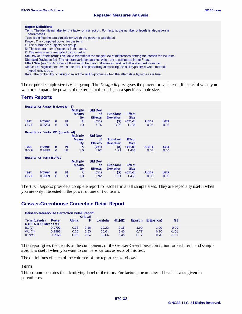
Report Definitions Term: The identifying label for the factor or interaction. For factors, the number of levels is also given in parentheses. Test: Identifies the test statistic for which the power is calculated. Power: The computed power for the term. n: The number of subjects per group. N: The total number of subjects in the study. K: The means were multiplied by this value. Std Dev of Effects (σm): This value represents the magnitude of differences among the means for the term. Standard Deviation (σ): The random variation against which σm is compared in the F test. Effect Size (σm/σ): An index of the size of the mean differences relative to the standard deviation. Alpha: The significance level of the test. The probability of rejecting the null hypothesis when the null hypothesis is true. Beta: The probability of failing to reject the null hypothesis when the alternative hypothesis is true.
The required sample size is 6 per group. The Design Report gives the power for each term. It is useful when you want to compare the powers of the terms in the design at a specific sample size.
Term Reports
Results for Factor B (Levels = 3) Multiply Std Dev Means of Standard Effect By Effects Deviation Size Test Power n N K (σm) (σ) (σm/σ) Alpha Beta GG F 0.9793 6 18 1.0 3.74 3.29 1.136 0.05 0.02 Results for Factor W1 (Levels =4) Multiply Std Dev Means of Standard Effect By Effects Deviation Size Test Power n N K (σm) (σ) (σm/σ) Alpha Beta GG F 0.9998 6 18 1.0 1.92 1.31 1.465 0.05 0.00 Results for Term B1*W1 Multiply Std Dev Means of Standard Effect By Effects Deviation Size Test Power n N K (σm) (σ) (σm/σ) Alpha Beta GG F 0.9969 6 18 1.0 1.92 1.31 1.465 0.05 0.00
The Term Reports provide a complete report for each term at all sample sizes. They are especially useful when you are only interested in the power of one or two terms.
Geisser-Greenhouse Correction Detail Report
Geisser-Greenhouse Correction Detail Report Critical Term (Levels) Power Alpha F Lambda df1|df2 Epsilon E(Epsilon) G1 n = 6 N = 18 Means x 1 B1 (3) 0.9793 0.05 3.68 23.23 2|15 1.00 1.00 0.00 W1 (4) 0.9998 0.05 3.25 38.64 3|45 0.77 0.70 -1.01 B1*W1 0.9969 0.05 2.64 38.64 6|45 0.77 0.70 -1.01
This report gives the details of the components of the Geisser-Greenhouse correction for each term and sample size. It is useful when you want to compare various aspects of this test.
The definitions of each of the columns of the report are as follows.
Term This column contains the identifying label of the term. For factors, the number of levels is also given in parentheses.
PASS Sample Size Software NCSS.com Repeated Measures Analysis
570-33 © NCSS, LLC. All Rights Reserved.
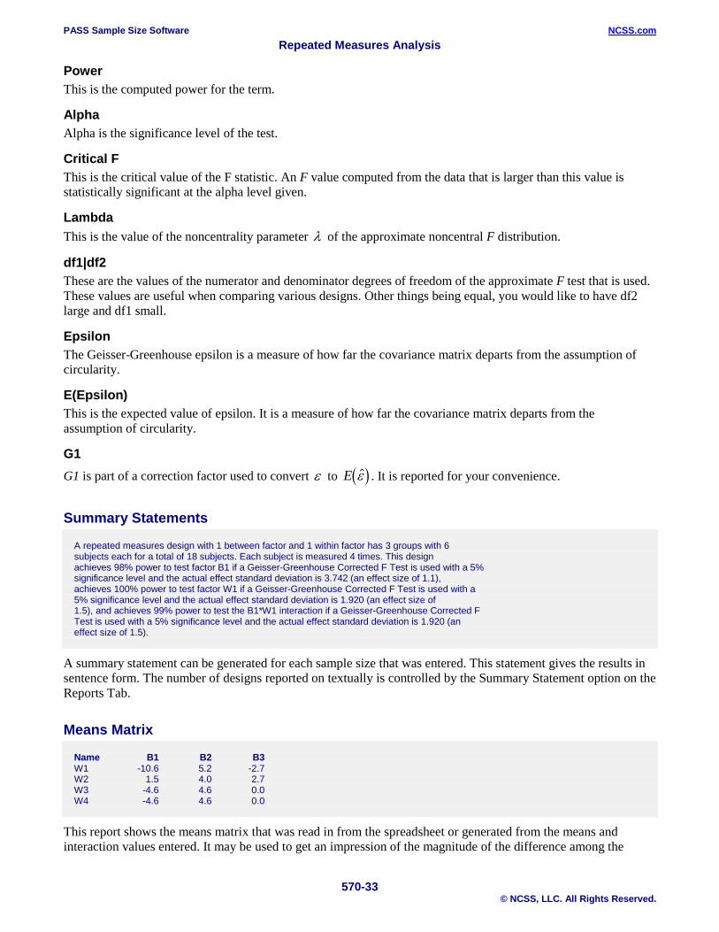
Power This is the computed power for the term.
Alpha Alpha is the significance level of the test.
Critical F This is the critical value of the F statistic. An F value computed from the data that is larger than this value is statistically significant at the alpha level given.
Lambda This is the value of the noncentrality parameter λ of the approximate noncentral F distribution.
df1|df2 These are the values of the numerator and denominator degrees of freedom of the approximate F test that is used. These values are useful when comparing various designs. Other things being equal, you would like to have df2 large and df1 small.
Epsilon The Geisser-Greenhouse epsilon is a measure of how far the covariance matrix departs from the assumption of circularity.
E(Epsilon) This is the expected value of epsilon. It is a measure of how far the covariance matrix departs from the assumption of circularity.
G1 G1 is part of a correction factor used to convert ε to ( )E ε . It is reported for your convenience.
Summary Statements
A repeated measures design with 1 between factor and 1 within factor has 3 groups with 6 subjects each for a total of 18 subjects. Each subject is measured 4 times. This design achieves 98% power to test factor B1 if a Geisser-Greenhouse Corrected F Test is used with a 5% significance level and the actual effect standard deviation is 3.742 (an effect size of 1.1), achieves 100% power to test factor W1 if a Geisser-Greenhouse Corrected F Test is used with a 5% significance level and the actual effect standard deviation is 1.920 (an effect size of 1.5), and achieves 99% power to test the B1*W1 interaction if a Geisser-Greenhouse Corrected F Test is used with a 5% significance level and the actual effect standard deviation is 1.920 (an effect size of 1.5).
A summary statement can be generated for each sample size that was entered. This statement gives the results in sentence form. The number of designs reported on textually is controlled by the Summary Statement option on the Reports Tab.
Means Matrix
Name B1 B2 B3 W1 -10.6 5.2 -2.7 W2 1.5 4.0 2.7 W3 -4.6 4.6 0.0 W4 -4.6 4.6 0.0
This report shows the means matrix that was read in from the spreadsheet or generated from the means and interaction values entered. It may be used to get an impression of the magnitude of the difference among the
PASS Sample Size Software NCSS.com Repeated Measures Analysis
570-34 © NCSS, LLC. All Rights Reserved.
means that is being studied. When a Means Multiplier, K, is used, each value of K is multiplied times each value of this matrix.
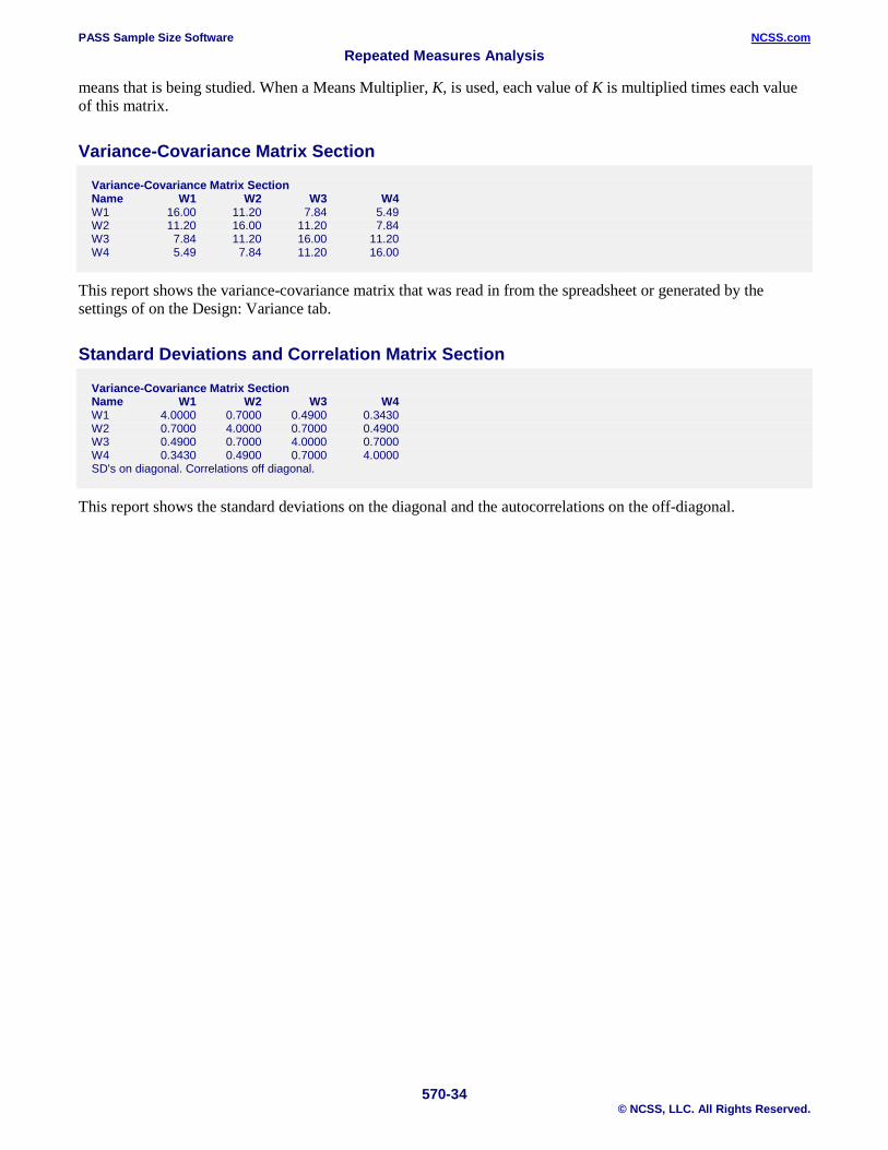
Variance-Covariance Matrix Section
Variance-Covariance Matrix Section Name W1 W2 W3 W4 W1 16.00 11.20 7.84 5.49 W2 11.20 16.00 11.20 7.84 W3 7.84 11.20 16.00 11.20 W4 5.49 7.84 11.20 16.00
This report shows the variance-covariance matrix that was read in from the spreadsheet or generated by the settings of on the Design: Variance tab.
Standard Deviations and Correlation Matrix Section
Variance-Covariance Matrix Section Name W1 W2 W3 W4 W1 4.0000 0.7000 0.4900 0.3430 W2 0.7000 4.0000 0.7000 0.4900 W3 0.4900 0.7000 4.0000 0.7000 W4 0.3430 0.4900 0.7000 4.0000 SD's on diagonal. Correlations off diagonal.
This report shows the standard deviations on the diagonal and the autocorrelations on the off-diagonal.

PASS Sample Size Software NCSS.com Repeated Measures Analysis
570-35 © NCSS, LLC. All Rights Reserved.
Example 2 – Varying the Difference between the Means Continuing with Example 1, the researchers want to evaluate the impact on power of varying the size of the difference among the means for a range of sample sizes from 2 to 8 per groups. The researchers could try calculating various multiples of the means, inputting them, and recording the results. However, this can be accomplished directly by using the K option.
Keeping all other settings as in Example 2, the value of K is varied from 0.2 to 3.0 in steps of 0.2. We determined these values by experimentation so that a full range of power values are shown on the plots.
In the output to follow, we only display the plots. You may want to display the numeric reports as well, but we do not here in order to save space.
Setup This section presents the values of each of the parameters needed to run this example. First, from the PASS Home window, load the Repeated Measures Analysis procedure. You may then make the appropriate entries as listed below, or open Example 2 by going to the File menu and choosing Open Example Template.
Option Value Design: Means Tab Solve For ................................................ Power Tests Univariate: Geisser-Greenhouse ............ Checked
Alpha Alpha for All Terms ................................. 0.05
Design and Effects Number of Factors .................................. 1 Between, 1 Within Mean Input Type ..................................... Means, Interaction Effects
Factor B1 Levels ..................................................... 3 Means ..................................................... List of Means List of Means .......................................... 93 87 84
Factor W1 Levels ..................................................... 4 Means ..................................................... List of Means List of Means .......................................... 93 89 88 91 Effect Multipliers K’s (Multipliers) ....................................... 0.2 to 3.0 by 0.2 Sample Size Group Allocation ..................................... Equal (n1 = n2 = … = n) n (Subjects Per Group) ........................... 2 3 4 8
Interactions Tab Effects of Interaction Terms Enter B1*W1 Effects As .......................... Multiple of Another Term Multiplier ................................................. 1.0 Term........................................................ W1

PASS Sample Size Software NCSS.com Repeated Measures Analysis
570-36 © NCSS, LLC. All Rights Reserved.
Variances Tab Input Type ............................................... Non-Constant σ’s and ρ’s Standard Deviation Structure Pattern .................................................... Constant σ σ .............................................................. 4 Autocorrelation Structure Factor W1 ............................................... AR(1) ρ .............................................................. 0.7
Reports Tab Numeric Results by Term ....................... Not Checked Numeric Results by Design .................... Not Checked References ............................................. Not Checked Definitions ............................................... Not Checked Geisser-Greenhouse Detail Report ........ Not Checked Means Matrix .......................................... Not Checked Variance-Covariance Matrix ................... Not Checked SD and Autocorrelation Matrix ................ Not Checked Summary Statements ............................. Not Checked
Plots Tab Plots of Power vs n by Terms ................. Not Checked Plots of Power vs K by n ......................... Checked
Output Click the Calculate button to perform the calculations and generate the following output.
Plots Section

PASS Sample Size Software NCSS.com Repeated Measures Analysis
570-37 © NCSS, LLC. All Rights Reserved.
These charts show how the power depends on the relative size of the means as well as the group sample size n.

PASS Sample Size Software NCSS.com Repeated Measures Analysis
570-38 © NCSS, LLC. All Rights Reserved.
Example 3 – Power after a Study This example will show how to calculate the power of F tests from data that have already been collected and analyzed using the analysis of variance. The following results were obtained using the analysis of variance procedure in NCSS. In this example, Gender is the between factor with two levels and Treatment is the within factor with three levels. The experiment was conducted with two subjects per group, but there is interest in the power for 2, 3, and 4 subjects per group. All tests use a significance level of 0.05. Analysis of Variance Table
Source Sum of Mean Prob Term DF Squares Square F-Ratio Level A (Gender) 1 21.33333 21.33333 32.00 0.029857 B(A) 2 1.333333 0.6666667 C (Treatment) 2 5.166667 2.583333 6.20 0.059488 AC 2 5.166667 2.583333 6.20 0.059488 BC(A) 4 1.666667 0.4166667 Total (Adjusted) 11 34.66667 Total 12 Means and Effects Section Standard Term Count Mean Error All 12 17.33333 A: Gender Females 6 16 0.3333333 Males 6 18.66667 0.3333333 C: Treatment L 4 16.75 0.3227486 M 4 17 0.3227486 H 4 18.25 0.3227486 AC: Gender,Treatment Females,L 2 14.5 0.4564355 Females,M 2 16 0.4564355 Females,H 2 17.5 0.4564355 Males,L 2 19 0.4564355 Males,M 2 18 0.4564355 Males,H 2 19 0.4564355
Note that the treatment means (L, M, and H) show an increasing pattern from 16.75 to 18.25, but the hypothesis test of this factor is not statistically significant at the 0.05 level. We will now calculate the power of the three F tests using PASS. We will use the regular F test since that is what was used in the above table.
Using the means from the table, the following means matrix is created.
14.5 19 16 18 17.5 19
From the printout, we note that MSB = 0.6666667 and MSW = 0.4166667. Plugging these values into the estimating equations
( )ρ = −
+ −MSB MSW
MSB T MSW1
σρ
2
1=
−MSW
yields
. .
. ( ) ..ρ = −
+ −=
0 6666667 0 41666670 6666667 3 1 0 4166667
016666667

PASS Sample Size Software NCSS.com Repeated Measures Analysis
570-39 © NCSS, LLC. All Rights Reserved.
..
.σ 2 0 41666671 016666667
0 5=−
=
so that
. .σ = =05 0 70710681
With these values calculated, we can setup PASS to calculate the power of the three F tests as follows.
Setup This section presents the values of each of the parameters needed to run this example. First, from the PASS Home window, load the Repeated Measures Analysis procedure. You may then make the appropriate entries as listed below, or open Example 3 by going to the File menu and choosing Open Example Template.
Option Value Design: Means Tab Solve For ................................................ Power Tests Univariate: F Test ................................... Checked
Alpha Alpha for All Terms ................................. 0.05
Design and Effects Number of Factors .................................. 1 Between, 1 Within Mean Input Type ..................................... Means in Spreadsheet Factor B1 Levels ..................................................... 2
Factor W1 Levels ..................................................... 3 Columns Containing the Means ............. C1-C2 Press the Spreadsheet button to enter the following values into the spreadsheet
Row 1 ...................................................... 14.5 19.0 Row 2 ...................................................... 16.0 18.0 Row 3 ...................................................... 17.5 19.0 Effect Multipliers K’s (Multipliers) ....................................... 1 Sample Size Group Allocation ..................................... Equal (n1 = n2 = … = n) n (Subjects Per Group) ........................... 2 3 4
Variances Tab Input Type ............................................... Constant σ and ρ Constant σ and ρ σ .............................................................. 0.70710681 ρ .............................................................. 0.16667

PASS Sample Size Software NCSS.com Repeated Measures Analysis
570-40 © NCSS, LLC. All Rights Reserved.
Reports Tab Numeric Results by Term ....................... Not Checked Numeric Results by Design .................... Checked References ............................................. Not Checked Definitions ............................................... Not Checked Geisser-Greenhouse Detail Report ........ Not Checked Means Matrix .......................................... Not Checked Variance-Covariance Matrix ................... Not Checked SD and Autocorrelation Matrix ................ Not Checked Summary Statements ............................. Not Checked
Plots Tab Plots of Power vs n by Terms ................. Not Checked Plots of Power vs K by n ......................... Not Checked
Output Click the Calculate button to perform the calculations and generate the following output.
Numeric Results
Multiply Std Dev Means of Standard Effect By Effects Deviation Size Term Test Power n N K (σm) (σ) (σm/σ) Alpha Beta B1(2) F 0.8004 2 4 1.0 1.33 0.47 2.828 0.05 0.20 W1(3) F 0.5536 2 4 1.0 0.66 0.37 1.761 0.05 0.45 B1*W1 F 0.5536 2 4 1.0 0.66 0.37 1.761 0.05 0.45 B1(2) F 0.9985 3 6 1.0 1.33 0.47 2.828 0.05 0.00 W1(3) F 0.8933 3 6 1.0 0.66 0.37 1.761 0.05 0.11 B1*W1 F 0.8933 3 6 1.0 0.66 0.37 1.761 0.05 0.11 B1(2) F 1.0000 4 8 1.0 1.33 0.47 2.828 0.05 0.00 W1(3) F 0.9801 4 8 1.0 0.66 0.37 1.761 0.05 0.02 B1*W1 F 0.9801 4 8 1.0 0.66 0.37 1.761 0.05 0.02
You can see that the power of the tests on W1 and B1*W1 is only 0.5536 for an n of 2. However, if n is 3, a much more reasonable power of 0.8933 is achieved.
PASS Sample Size Software NCSS.com Repeated Measures Analysis
570-41 © NCSS, LLC. All Rights Reserved.
Example 4 – Cross-Over Design A crossover design is a special type of repeated measures design in which the treatments are applied to the subjects in different orders. The between-subjects (grouping) factor is defined by the specific sequence in which the treatments are applied. For example, suppose the treatments are represented by B1 and B2. Further suppose that half the subjects receive treatment B1 followed by treatment B2 (sequence B1B2), while the other half receive treatment B2 followed by treatment B1 (sequence B2B1). This is a two-group crossover design.
Crossover designs assume that a long enough period elapses between measurements so that the effects of one treatment are washed out before the next treatment is applied. This is known as the assumption of no carryover effects.
When a crossover design is analyzed using repeated measures, the interaction is the only term of interest. The F test of the between factor tests whether means across each sequence are equal—a test of secondary interest. The F test of the within factor tests whether the response is different across the time periods—also of secondary interest. The F test for interaction tests whether the change in response across time is the same for both sequences. The interaction can only be significant if the treatments effect the outcome differently. Hence, to specify a crossover design requires the careful specification of the interaction effects.
With this background, we present an example. Suppose researchers want to investigate the reduction in heart-beat rate caused by the administration of a certain drug using a simple two-period crossover design. The researchers want a sample size large enough to detect a drop in heart-beat rate from 95 to 90 with a power of 90% at the 0.05 significance level. Previous studies have shown a within-patient autocorrelation of 0.50 and a standard deviation of 3.98.
The hypothesized interaction is calculated using the Standard Deviation of Means Calculator tool. This window is loaded using the Sm icon to the right of the ‘Number of Factors’ box, or by selecting ‘Means to Sm Estimator’ from the Tools menu.
Once this tool is displayed, enter the four treatment heart-beat rates forming a 2 by 2 matrix as follows:
95 90
90 95
The required standard deviation of the interaction effects will be displayed at the bottom of the window as the value of Sm(AB), which is 2.5.
Setup This section presents the values of each of the parameters needed to run this example. First, from the PASS Home window, load the Repeated Measures Analysis procedure. You may then make the appropriate entries as listed below, or open Example 4 by going to the File menu and choosing Open Example Template.
Option Value Design: Means Tab Solve For ................................................ Sample Size Based on ................................................. F-Test Term........................................................ B1*W1 Tests Univariate: F Test ................................... Checked
Power and Alpha Minimum Power ...................................... 0.90 Alpha for All Terms ................................. 0.05

PASS Sample Size Software NCSS.com Repeated Measures Analysis
570-42 © NCSS, LLC. All Rights Reserved.
Design and Effects Number of Factors .................................. 1 Between, 1 Within Mean Input Type ..................................... Means, Interaction Effects
Factor B1 Levels ..................................................... 2 Means ..................................................... List of Means List of Means .......................................... 90 95 (these values are ignored)
Factor W1 Levels ..................................................... 2 Means ..................................................... List of Means List of Means .......................................... 90 95 (these values are ignored) Effect Multipliers K’s (Multipliers) ....................................... 1 Sample Size Group Allocation ..................................... Equal (n1 = n2 = …)
Interactions Tab Effects of Interaction Terms Enter Effects As ...................................... Standard Deviation Value ....................................................... 2.5
Variances Tab Input Type ............................................... Constant σ and ρ Constant σ and ρ σ .............................................................. 3.98 ρ .............................................................. 0.5
Reports Tab Numeric Results by Term ....................... Not Checked Numeric Results by Design .................... Checked References ............................................. Not Checked Definitions ............................................... Not Checked Geisser-Greenhouse Detail Report ........ Not Checked Means Matrix .......................................... Not Checked Variance-Covariance Matrix ................... Not Checked SD and Autocorrelation Matrix ................ Not Checked Summary Statements ............................. Not Checked
Plots Tab Plots of Power vs n by Terms ................. Not Checked Plots of Power vs K by n ......................... Not Checked

PASS Sample Size Software NCSS.com Repeated Measures Analysis
570-43 © NCSS, LLC. All Rights Reserved.
Output Click the Calculate button to perform the calculations and generate the following output.
Numeric Results Multiply Std Dev Means of Standard Effect By Effects Deviation Size Term Test Power n N K (σm) (σ) (σm/σ) Alpha Beta B1(2) F 0.5224 5 10 1.0 2.50 3.45 0.725 0.05 0.48 W1(2) F 0.9338 5 10 1.0 2.50 1.99 1.256 0.05 0.07 B1*W1 F 0.9338 5 10 1.0 2.50 1.99 1.256 0.05 0.07
We only display the interaction term since that is the only term of interest. We note that 90% power is achieved when n is 5. This corresponds to a total sample size of 10 subjects.

PASS Sample Size Software NCSS.com Repeated Measures Analysis
570-44 © NCSS, LLC. All Rights Reserved.
Example 5 – Power of a Completed Cross-Over Design The following analysis of variance table was generated by NCSS for a set of crossover data. Find the power of the interaction F test assuming a significance level of 0.05.
Analysis of Variance Table Source Sum of Mean Prob Term DF Squares Square F-Ratio Level A: Sequence 1 89397.6 89397.6 1.19 0.285442 B(A): Subject 28 2110739 75383.54 C: Period 1 117395.3 117395.3 1.40 0.246854 AC 1 122401.7 122401.7 1.46 0.237263 BC(A) 28 2349752 83919.72 Total (Adjusted) 59 4789686 Total 60 Means Section Standard Term Count Mean Error All 60 492.2000 A: Sequence 1 30 453.6000 50.12768 2 30 530.8000 50.12768 C: Period 1 30 447.9667 52.88973 2 30 536.4333 52.88973 AC: Sequence,Period 1,1 15 364.2000 74.79738 1,2 15 543.0000 74.79738 2,1 15 531.7333 74.79738 2,2 15 529.8666 74.79738
One difficulty in analyzing an existing crossover design is determining an appropriate value for the hypothesized interaction effects. One method is to find the standard deviation of the interaction effects by taking the square root of the Sum of Squares for the interaction divided by the total number of observations. In this case,
σ Interaction =
=
122401760
451667
.
.
Another method is to find the individual interaction effects by subtraction. This method proceeds as follows.
First, subtract the Period means from the Sequence by Period means.
364 2000 53173335430000 529 8666
447 9667536 4333
837667 8376676 5667 6 5667
. .
. ...
. .
. .
−
=
−−
Next, compute the column means and subtract them from the current values. This results in the effects.
−−
−
−−
=
−−
837667 8376676 5667 6 5667
38 6000 38 600038 6000 38 6000
451667 451667451667 451667
. .
. .. .. .
. .
. .
Finally, compute the standard deviation of the effects. Since the mean of the effects is zero, the standard deviation is
( ) ( ) ( ) ( )σ Interaction =− + + + −
=
451667 451667 451667 4516674
451667
2 2 2 2. . . .
.

PASS Sample Size Software NCSS.com Repeated Measures Analysis
570-45 © NCSS, LLC. All Rights Reserved.
Another difficulty that must be solved is to estimate the autocorrelation and within-subject standard deviation. From the above printout, we note that MSB = 75383.54 and MSW = 83919.72. Plugging these values into the estimating equations
( )ρ = −
+ −MSB MSW
MSB T MSW1
σρ
2
1=
−MSW
yields
. .
. ( ) ..ρ = −
+ −= −
7538354 83919 727538354 2 1 83919 72
0 05358447
.
..σ 2 83919 72
1 0 053584477965163=
+=
so that
. .σ = =7965163 282 2262
Setup This section presents the values of each of the parameters needed to run this example. First, from the PASS Home window, load the Repeated Measures Analysis procedure. You may then make the appropriate entries as listed below, or open Example 5 by going to the File menu and choosing Open Example Template.
Option Value Design: Means Tab Solve For ................................................ Power Tests Univariate: Geisser-Greenhouse ............ Checked
Alpha Alpha for All Terms ................................. 0.05
Design and Effects Number of Factors .................................. 1 Between, 1 Within Mean Input Type ..................................... Means, Interaction Effects
Factor B1 Levels ..................................................... 2 Means ..................................................... List of Means List of Means .......................................... 453.6 530.8
Factor W1 Levels ..................................................... 2 Means ..................................................... List of Means List of Means .......................................... 447.9667 536.4333 Effect Multipliers K’s (Multipliers) ....................................... 1
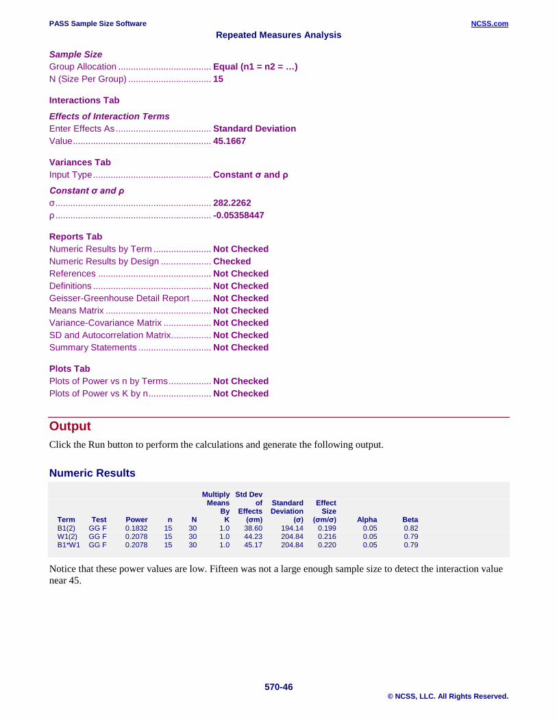
PASS Sample Size Software NCSS.com Repeated Measures Analysis
570-46 © NCSS, LLC. All Rights Reserved.
Sample Size Group Allocation ..................................... Equal (n1 = n2 = …) N (Size Per Group) ................................. 15
Interactions Tab Effects of Interaction Terms Enter Effects As ...................................... Standard Deviation Value ....................................................... 45.1667
Variances Tab Input Type ............................................... Constant σ and ρ Constant σ and ρ σ .............................................................. 282.2262 ρ .............................................................. -0.05358447
Reports Tab Numeric Results by Term ....................... Not Checked Numeric Results by Design .................... Checked References ............................................. Not Checked Definitions ............................................... Not Checked Geisser-Greenhouse Detail Report ........ Not Checked Means Matrix .......................................... Not Checked Variance-Covariance Matrix ................... Not Checked SD and Autocorrelation Matrix ................ Not Checked Summary Statements ............................. Not Checked
Plots Tab Plots of Power vs n by Terms ................. Not Checked Plots of Power vs K by n ......................... Not Checked
Output Click the Run button to perform the calculations and generate the following output.
Numeric Results
Multiply Std Dev Means of Standard Effect By Effects Deviation Size Term Test Power n N K (σm) (σ) (σm/σ) Alpha Beta B1(2) GG F 0.1832 15 30 1.0 38.60 194.14 0.199 0.05 0.82 W1(2) GG F 0.2078 15 30 1.0 44.23 204.84 0.216 0.05 0.79 B1*W1 GG F 0.2078 15 30 1.0 45.17 204.84 0.220 0.05 0.79
Notice that these power values are low. Fifteen was not a large enough sample size to detect the interaction value near 45.

PASS Sample Size Software NCSS.com Repeated Measures Analysis
570-47 © NCSS, LLC. All Rights Reserved.
Example 6 – Validation using O’Brien and Muller O’Brien and Muller’s article in the book edited by Edwards (1993) analyze the power of a two-group repeated-measures experiment in which three measurements are made on each subject.
The hypothesized means are
Group 1 Group 2 Time 1 3 1 Time 2 12 5 Time 3 8 7
The covariance matrix is
Time 1 Time 2 Time 3 Time 1 25 16 12 Time 2 16 64 30 Time 3 12 30 36
With n’s of 12, 18, and 24 and an alpha of 0.05, they obtained power values using the Wilks’ Lambda test. Their reported power values are
Power Values for each Term n Group Time Interaction 12 0.326 0.983 0.461 18 0.467 0.999 0.671 24 0.589 0.999 0.814
O’Brien, in a private communication, re-ran these data using the Geisser-Greenhouse correction. His results were as follows:
Power Values for each Term n Group Time Interaction 12 0.326 0.993 0.486 18 0.467 0.999 0.685 24 0.589 0.999 0.819
Setup This section presents the values of each of the parameters needed to run this example. First, from the PASS Home window, load the Repeated Measures Analysis procedure. You may then make the appropriate entries as listed below, or open Example 6 by going to the File menu and choosing Open Example Template.
Option Value Design: Means Tab Solve For ................................................ Power Tests Univariate: Geisser-Greenhouse ............ Checked Multivariate: Wilks’ Lambda .................... Checked
Alpha Alpha for All Terms ................................. 0.05

PASS Sample Size Software NCSS.com Repeated Measures Analysis
570-48 © NCSS, LLC. All Rights Reserved.
Design and Effects Number of Factors .................................. 1 Between, 1 Within Mean Input Type ..................................... Means in Spreadsheet Factor B1 Levels ..................................................... 2
Factor W1 Levels ..................................................... 3 Columns Containing the Means ............. C1-C2 Press the Spreadsheet button to enter the following values into columns 1 and 2 of the spreadsheet
Row 1 ...................................................... 3 1 Row 2 ...................................................... 12 5 Row 3 ...................................................... 8 7 Effect Multipliers K’s (Multipliers) ....................................... 1 Sample Size Group Allocation ..................................... Equal (n1 = n2 = … = n) n (Subjects Per Group) ........................... 12 18 24
Variances Tab Input Type ............................................... Variance-Covariance Matrix in Spreadsheet Variance-Covariance Matrix in Spreadsheet Columns Containing Covariance Matrix . C4-C6 Press the Spreadsheet button to enter the following values into columns 4, 5, and 6 of the spreadsheet.
Row 1 ...................................................... 25 16 12 Row 2 ...................................................... 16 64 30 Row 3 ...................................................... 12 30 36
Reports Tab Numeric Results by Term ....................... Checked Numeric Results by Design .................... Not Checked References ............................................. Not Checked Definitions ............................................... Not Checked Geisser-Greenhouse Detail Report ........ Not Checked Means Matrix .......................................... Not Checked Variance-Covariance Matrix ................... Not Checked SD and Autocorrelation Matrix ................ Not Checked Summary Statements ............................. Not Checked
Plots Tab Plots of Power vs n by Terms ................. Not Checked Plots of Power vs K by n ......................... Not Checked
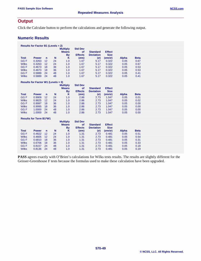
PASS Sample Size Software NCSS.com Repeated Measures Analysis
570-49 © NCSS, LLC. All Rights Reserved.
Output Click the Calculate button to perform the calculations and generate the following output.
Numeric Results Results for Factor B1 (Levels = 2) Multiply Std Dev Means of Standard Effect By Effects Deviation Size Test Power n N K (σm) (σ) (σm/σ) Alpha Beta GG F 0.3263 12 24 1.0 1.67 5.17 0.322 0.05 0.67 Wilks 0.3263 12 24 1.0 1.67 5.17 0.322 0.05 0.67 GG F 0.4673 18 36 1.0 1.67 5.17 0.322 0.05 0.53 Wilks 0.4673 18 36 1.0 1.67 5.17 0.322 0.05 0.53 GG F 0.5889 24 48 1.0 1.67 5.17 0.322 0.05 0.41 Wilks 0.5889 24 48 1.0 1.67 5.17 0.322 0.05 0.41 Results for Factor W1 (Levels = 3) Multiply Std Dev Means of Standard Effect By Effects Deviation Size Test Power n N K (σm) (σ) (σm/σ) Alpha Beta GG F 0.9909 12 24 1.0 2.86 2.73 1.047 0.05 0.01 Wilks 0.9825 12 24 1.0 2.86 2.73 1.047 0.05 0.02 GG F 0.9997 18 36 1.0 2.86 2.73 1.047 0.05 0.00 Wilks 0.9995 18 36 1.0 2.86 2.73 1.047 0.05 0.00 GG F 1.0000 24 48 1.0 2.86 2.73 1.047 0.05 0.00 Wilks 1.0000 24 48 1.0 2.86 2.73 1.047 0.05 0.00
Results for Term B1*W1 Multiply Std Dev Means of Standard Effect By Effects Deviation Size Test Power n N K (σm) (σ) (σm/σ) Alpha Beta GG F 0.4822 12 24 1.0 1.31 2.73 0.481 0.05 0.51 Wilks 0.4605 12 24 1.0 1.31 2.73 0.481 0.05 0.54 GG F 0.6810 18 36 1.0 1.31 2.73 0.481 0.05 0.31 Wilks 0.6706 18 36 1.0 1.31 2.73 0.481 0.05 0.33 GG F 0.8157 24 48 1.0 1.31 2.73 0.481 0.05 0.18 Wilks 0.8136 24 48 1.0 1.31 2.73 0.481 0.05 0.19
PASS agrees exactly with O’Brien’s calculations for Wilks tests results. The results are slightly different for the Geisser-Greenhouse F tests because the formulas used to make these calculation have been upgraded.

PASS Sample Size Software NCSS.com Repeated Measures Analysis
570-50 © NCSS, LLC. All Rights Reserved.
Example 7 – Unequal Group Sizes Usually, in the planning stages, the group sample sizes are equal. Occasionally, however, you may want to plan for a situation in which one group will have a larger sample size than the others. Also, when doing a power analysis on a study that has already been conducted, the group sample sizes are often unequal.
In this example, we will re-analyze the Example 3. However, we will now assume that there were four subjects in group 1 and eight subjects in group 2. The setup and output for this example are as follows.
Setup This section presents the values of each of the parameters needed to run this example. First, from the PASS Home window, load the Repeated Measures Analysis procedure. You may then make the appropriate entries as listed below, or open Example 7 by going to the File menu and choosing Open Example Template.
Option Value Design: Means Tab Solve For ................................................ Power Tests Univariate: F Test ................................... Checked
Alpha Alpha for All Terms ................................. 0.05
Design and Effects Number of Factors .................................. 1 Between, 1 Within Mean Input Type ..................................... Means in Spreadsheet Factor B1 Levels ..................................................... 2
Factor W1 Levels ..................................................... 3 Columns Containing the Means ............. C1-C2 Press the Spreadsheet button to enter the following values into the spreadsheet
Row 1 ...................................................... 14.5 19.0 Row 2 ...................................................... 16.0 18.0 Row 3 ...................................................... 17.5 19.0 Effect Multipliers K’s (Multipliers) ....................................... 1 Sample Size Group Allocation ..................................... Unequal (n1, n2, … Individually) n1, n2, … (List) ....................................... 4 8
Variances Tab Input Type ............................................... Constant σ and ρ Constant σ and ρ σ .............................................................. 0.70710681 ρ .............................................................. 0.16667
Reports Tab Numeric Results by Term ....................... Not Checked
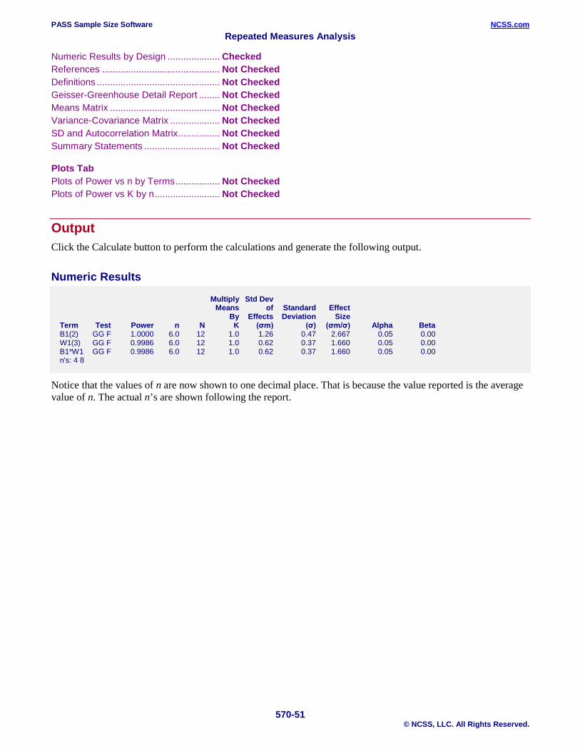
PASS Sample Size Software NCSS.com Repeated Measures Analysis
570-51 © NCSS, LLC. All Rights Reserved.
Numeric Results by Design .................... Checked References ............................................. Not Checked Definitions ............................................... Not Checked Geisser-Greenhouse Detail Report ........ Not Checked Means Matrix .......................................... Not Checked Variance-Covariance Matrix ................... Not Checked SD and Autocorrelation Matrix ................ Not Checked Summary Statements ............................. Not Checked
Plots Tab Plots of Power vs n by Terms ................. Not Checked Plots of Power vs K by n ......................... Not Checked
Output Click the Calculate button to perform the calculations and generate the following output.
Numeric Results Multiply Std Dev Means of Standard Effect By Effects Deviation Size Term Test Power n N K (σm) (σ) (σm/σ) Alpha Beta B1(2) GG F 1.0000 6.0 12 1.0 1.26 0.47 2.667 0.05 0.00 W1(3) GG F 0.9986 6.0 12 1.0 0.62 0.37 1.660 0.05 0.00 B1*W1 GG F 0.9986 6.0 12 1.0 0.62 0.37 1.660 0.05 0.00 n's: 4 8
Notice that the values of n are now shown to one decimal place. That is because the value reported is the average value of n. The actual n’s are shown following the report.

PASS Sample Size Software NCSS.com Repeated Measures Analysis
570-52 © NCSS, LLC. All Rights Reserved.
Example 8 – Designs with more than Two Factors Occasionally, you will have a design that has more than two factors. We will now show you how to compute the necessary sample size for such a design.
Suppose your design calls for two between-subject factors, Age (A) and Gender (G), and two within-subject factors, dose-level (D) and application method (M). The number of levels of these four factors are, respectively, 3, 2, 4, and 2.
Our first task is to determine appropriate effect values for each of the terms. We decide to ignore the interactions during the planning and only consider the factors themselves. The desired difference to be detected among the three age groups can be represented by the means 80, 88, and 96. The desired difference to be detected among the two genders can be represented by the means 80 and 96. The desired difference to be detected among the four dose levels is represented by the means 80, 82, 84, and 86. The desired difference to be detected among the two application methods is represented by the means 80 and 86.
Our next task is to specify the covariance matrix. From previous experience, we have found that a constant value of 20.0 is appropriate for the standard deviation.
The autocorrelation pattern is more complex because there are two types of within factors. We need to understand how the measurements will be obtained to come up with a realistic autocorrelation pattern. Suppose that the four doses are administered at four equal-spaced time points using application method 1, then again using application method 2. This suggests that an autoregressive autocorrelation pattern with ρ = 0.7 can be used for doses and a constant autocorrelation matrix with ρ = 0.5 can be used for application method. These two matrices can then be combined using a Kronecker product.
Finally, we decide to calculate the power using the Geisser-Greenhouse test at the following sample sizes: 2, 4, 6, 8, 10, 20, 30, and 40.
Setup This section presents the values of each of the parameters needed to run this example. First, from the PASS Home window, load the Repeated Measures Analysis procedure. You may then make the appropriate entries as listed below, or open Example 8 by going to the File menu and choosing Open Example Template.
Option Value Design: Means Tab Solve For ................................................ Power Tests Univariate: Geisser-Greenhouse ............ Checked
Alpha Alpha for All Terms ................................. 0.05
Design and Effects Number of Factors .................................. 2 Between, 2 Within Mean Input Type ..................................... Means, Interaction Effects
Factor B1 Levels ..................................................... 3 Means ..................................................... List of Means List of Means .......................................... 80 88 96
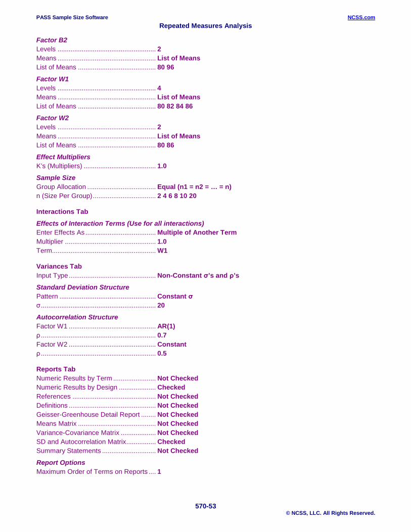
PASS Sample Size Software NCSS.com Repeated Measures Analysis
570-53 © NCSS, LLC. All Rights Reserved.
Factor B2 Levels ..................................................... 2 Means ..................................................... List of Means List of Means .......................................... 80 96
Factor W1 Levels ..................................................... 4 Means ..................................................... List of Means List of Means .......................................... 80 82 84 86 Factor W2 Levels ..................................................... 2 Means ..................................................... List of Means List of Means .......................................... 80 86 Effect Multipliers K’s (Multipliers) ....................................... 1.0 Sample Size Group Allocation ..................................... Equal (n1 = n2 = … = n) n (Size Per Group) .................................. 2 4 6 8 10 20
Interactions Tab Effects of Interaction Terms (Use for all interactions) Enter Effects As ...................................... Multiple of Another Term Multiplier ................................................. 1.0 Term........................................................ W1
Variances Tab Input Type ............................................... Non-Constant σ’s and ρ’s Standard Deviation Structure Pattern .................................................... Constant σ σ .............................................................. 20 Autocorrelation Structure Factor W1 ............................................... AR(1) ρ .............................................................. 0.7 Factor W2 ............................................... Constant ρ .............................................................. 0.5
Reports Tab Numeric Results by Term ....................... Not Checked Numeric Results by Design .................... Checked References ............................................. Not Checked Definitions ............................................... Not Checked Geisser-Greenhouse Detail Report ........ Not Checked Means Matrix .......................................... Not Checked Variance-Covariance Matrix ................... Not Checked SD and Autocorrelation Matrix ................ Checked Summary Statements ............................. Not Checked
Report Options Maximum Order of Terms on Reports .... 1

PASS Sample Size Software NCSS.com Repeated Measures Analysis
570-54 © NCSS, LLC. All Rights Reserved.
Plots Tab Plots of Power vs n by Terms ................. Checked Plots of Power vs K by n ......................... Not checked
Plot Options Maximum Order of Terms Plotted .......... 1
Output Click the Calculate button to perform the calculations and generate the following output.
Numeric Results Multiply Std Dev Means of Standard Effect By Effects Deviation Size Term Test Power n N K (σm) (σ) (σm/σ) Alpha Beta B1(3) GG F 0.1834 2 12 1.0 6.53 14.26 0.458 0.05 0.82 B2(2) GG F 0.3732 2 12 1.0 8.00 14.26 0.561 0.05 0.63 W1(4) GG F 0.1047 2 12 1.0 2.24 5.68 0.394 0.05 0.90 W2(2) GG F 0.1876 2 12 1.0 3.00 8.23 0.364 0.05 0.81 B1(3) GG F 0.4389 4 24 1.0 6.53 14.26 0.458 0.05 0.56 B2(2) GG F 0.7387 4 24 1.0 8.00 14.26 0.561 0.05 0.26 W1(4) GG F 0.2587 4 24 1.0 2.24 5.68 0.394 0.05 0.74 W2(2) GG F 0.3937 4 24 1.0 3.00 8.23 0.364 0.05 0.61 B1(3) GG F 0.6438 6 36 1.0 6.53 14.26 0.458 0.05 0.36 B2(2) GG F 0.9026 6 36 1.0 8.00 14.26 0.561 0.05 0.10 W1(4) GG F 0.3949 6 36 1.0 2.24 5.68 0.394 0.05 0.61 W2(2) GG F 0.5620 6 36 1.0 3.00 8.23 0.364 0.05 0.44 B1(3) GG F 0.7881 8 48 1.0 6.53 14.26 0.458 0.05 0.21 B2(2) GG F 0.9668 8 48 1.0 8.00 14.26 0.561 0.05 0.03 W1(4) GG F 0.5189 8 48 1.0 2.24 5.68 0.394 0.05 0.48 W2(2) GG F 0.6937 8 48 1.0 3.00 8.23 0.364 0.05 0.31 B1(3) GG F 0.8804 10 60 1.0 6.53 14.26 0.458 0.05 0.12 B2(2) GG F 0.9895 10 60 1.0 8.00 14.26 0.561 0.05 0.01 W1(4) GG F 0.6265 10 60 1.0 2.24 5.68 0.394 0.05 0.37 W2(2) GG F 0.7916 10 60 1.0 3.00 8.23 0.364 0.05 0.21 B1(3) GG F 0.9959 20 120 1.0 6.53 14.26 0.458 0.05 0.00 B2(2) GG F 1.0000 20 120 1.0 8.00 14.26 0.561 0.05 0.00 W1(4) GG F 0.9199 20 120 1.0 2.24 5.68 0.394 0.05 0.08 W2(2) GG F 0.9771 20 120 1.0 3.00 8.23 0.364 0.05 0.02 Standard Deviations and Correlation Matrix Section Name W1W1 W1W2 W2W1 W2W2 W3W1 W3W2 W4W1 W4W2 W1W1 20.0000 0.5000 0.7000 0.3500 0.4900 0.2450 0.3430 0.1715 W1W2 0.5000 20.0000 0.3500 0.7000 0.2450 0.4900 0.1715 0.3430 W2W1 0.7000 0.3500 20.0000 0.5000 0.7000 0.3500 0.4900 0.2450 W2W2 0.3500 0.7000 0.5000 20.0000 0.3500 0.7000 0.2450 0.4900 W3W1 0.4900 0.2450 0.7000 0.3500 20.0000 0.5000 0.7000 0.3500 W3W2 0.2450 0.4900 0.3500 0.7000 0.5000 20.0000 0.3500 0.7000 W4W1 0.3430 0.1715 0.4900 0.2450 0.7000 0.3500 20.0000 0.5000 W4W2 0.1715 0.3430 0.2450 0.4900 0.3500 0.7000 0.5000 20.0000 SD’s on diagonal. Correlations off diagonal.
This report gives the power values for the various terms and sample sizes that were entered. It also shows the autocorrelation pattern that resulted from the Kronecker product of the two within factor correlation matrices.
It is much easier to consider the following plot to interpret the results.
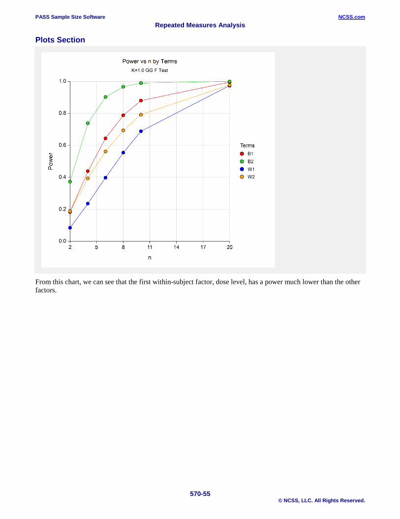
PASS Sample Size Software NCSS.com Repeated Measures Analysis
570-55 © NCSS, LLC. All Rights Reserved.
Plots Section
From this chart, we can see that the first within-subject factor, dose level, has a power much lower than the other factors.