remote source coding and awgn ceo problemsremote source coding and awgn ceo problems by krishnan...

Remote Source Coding and AWGN CEO Problems

Krishnan Eswaran

Electrical Engineering and Computer SciencesUniversity of California at Berkeley

Technical Report No. UCB/EECS-2006-2

http://www.eecs.berkeley.edu/Pubs/TechRpts/2006/EECS-2006-2.html

January 20, 2006

Copyright © 2006, by the author(s).All rights reserved.

Permission to make digital or hard copies of all or part of this work forpersonal or classroom use is granted without fee provided that copies arenot made or distributed for profit or commercial advantage and that copiesbear this notice and the full citation on the first page. To copy otherwise, torepublish, to post on servers or to redistribute to lists, requires prior specificpermission.


by

Krishnan Eswaran

B.S. Cornell University 2003

A thesis submitted in partial satisfactionof the requirements for the degree of

Master of Science, Plan II

in

Engineering - Electrical Engineering and Computer Sciences

in the

GRADUATE DIVISION

of the

UNIVERSITY OF CALIFORNIA, BERKELEY

Committee in charge:

Professor Michael GastparProfessor Kannan Ramchandran

Fall 2005


Copyright c© 2005

by

Krishnan Eswaran

Acknowledgements

I thank my advisors Michael Gastpar and Kannan Ramchandran for all their advice

and feedback while I was working on this. I would also like to thank Aaron Wagner

and Vinod Prabhakaran for discussions about converses to the CEO problem. In

particular, Aaron Wagner’s outer bound was instrumental in giving a non-trivial

lower bound to the sum-rate-distortion function for the AWGN CEO problem. Anand

Sarwate’s comments inspired the “no binning” results presented in this thesis. Vinod

Prabhakaran conveyed the results given in Section 4.4.2. Stimulating discussions with

Paolo Minero, Bobak Nazer, and Stark Draper are also gratefully acknowledged.

There are others who helped make writing this thesis a lot easier. Ruth Gjerde

went the extra mile to help with paperwork. Niels Hoven’s thesis template saved

me what would have been hours of formatting. Neelam Ihsanullah helped proofread

various incarnations of the writing. Finally, to everyone else that helped make my

life easier while I was working on this thesis, thanks for everything.

i

Contents

Contents ii

List of Figures iv

List of Tables v

1 Introduction 1

1.1 Mean Squared Error and Estimation . . . . . . . . . . . . . . . . . . 4

1.2 Background, Definitions, and Notation . . . . . . . . . . . . . . . . . 8

2 Remote Source Coding 13

2.1 Remote Rate-Distortion Function with a Single Observation . . . . . 14

2.2 Remote Rate-Distortion Function with Multiple Observations . . . . 17

2.3 Squared Error Distortion and Encoder Estimation . . . . . . . . . . . 19

2.4 Examples . . . . . . . . . . . . . . . . . . . . . . . . . . . . . . . . . 22

2.5 Discussion . . . . . . . . . . . . . . . . . . . . . . . . . . . . . . . . . 23

3 AWGN CEO Problems 24

3.1 Background and Notation . . . . . . . . . . . . . . . . . . . . . . . . 25

3.2 Lower Bound . . . . . . . . . . . . . . . . . . . . . . . . . . . . . . . 27

3.3 Upper Bounds . . . . . . . . . . . . . . . . . . . . . . . . . . . . . . . 29

3.3.1 Maximum Entropy Upper Bound . . . . . . . . . . . . . . . . 30

3.3.2 Rate Loss Upper Bound . . . . . . . . . . . . . . . . . . . . . 32

3.3.3 Rate Loss Upper Bound vs. Maximum Entropy Upper Bound 34

3.4 Discussion . . . . . . . . . . . . . . . . . . . . . . . . . . . . . . . . . 37

ii

4 Scaling Laws 38

4.1 Definitions and Notation . . . . . . . . . . . . . . . . . . . . . . . . . 39

4.2 Remote Source Coding Problem . . . . . . . . . . . . . . . . . . . . . 40

4.3 CEO Problem . . . . . . . . . . . . . . . . . . . . . . . . . . . . . . . 42

4.4 No Binning . . . . . . . . . . . . . . . . . . . . . . . . . . . . . . . . 44

4.4.1 Quadratic AWGN CEO Problem . . . . . . . . . . . . . . . . 46

4.4.2 Binary Erasure . . . . . . . . . . . . . . . . . . . . . . . . . . 48

4.5 Discussion . . . . . . . . . . . . . . . . . . . . . . . . . . . . . . . . . 50

5 Conclusion and Future Work 51

Bibliography 53

References . . . . . . . . . . . . . . . . . . . . . . . . . . . . . . . . . . . . 53

A Lower Bounds on MMSE 55

B Unified Entropy Power Inequality 59

B.1 Main Result . . . . . . . . . . . . . . . . . . . . . . . . . . . . . . . . 59

B.2 Definitions and Notation . . . . . . . . . . . . . . . . . . . . . . . . . 60

B.3 Fisher Information Inequalities . . . . . . . . . . . . . . . . . . . . . 62

B.4 Gaussian Smoothing . . . . . . . . . . . . . . . . . . . . . . . . . . . 64

C Sufficient Statistics in Remote Source Coding 67

C.1 Sufficient Statistics in Additive White Gaussian Noise . . . . . . . . . 67

C.2 Remote Rate-Distortion Functions . . . . . . . . . . . . . . . . . . . . 67

D Rate Loss 69

D.1 Definitions and Notation . . . . . . . . . . . . . . . . . . . . . . . . . 70

D.2 General Rate Loss Expression . . . . . . . . . . . . . . . . . . . . . . 71

E Linear Algebra 74

iii

List of Figures

1.1 Classical Source Coding . . . . . . . . . . . . . . . . . . . . . . . . . 1

1.2 Remote Source Coding . . . . . . . . . . . . . . . . . . . . . . . . . . 2

1.3 CEO Problem . . . . . . . . . . . . . . . . . . . . . . . . . . . . . . 3

1.4 Two Pulse Source. . . . . . . . . . . . . . . . . . . . . . . . . . . . . 7

2.1 Remote Source Coding with a Single Observation . . . . . . . . . . . 13

2.2 Remote Source Coding with M Observations . . . . . . . . . . . . . 14

2.3 Plot of bounds for Gaussian, Laplacian, and uniform sources . . . . . 22

3.1 AWGN CEO problem . . . . . . . . . . . . . . . . . . . . . . . . . . . 25

3.2 Plots for the Laplacian and uniform source in AWGN CEO problem. 31

3.3 When the curve crosses log(2), the rate loss approach provides a betterbound than the maximum entropy bound for the BPSK source andlarge enough M . . . . . . . . . . . . . . . . . . . . . . . . . . . . . . 34

3.4 The rate loss upper bound outperforms the maximum entropy upperbound for the BPSK source for certain distortions. . . . . . . . . . . . 36

4.1 Scaling behavior for Laplacian source in AWGN CEO Problem . . . 44

4.2 Scaling behavior for Logistic source in AWGN CEO Problem . . . . 45

A.1 Example of a source that decays as s−1. . . . . . . . . . . . . . . . . 56

B.1 Desired behavior of s(t) . . . . . . . . . . . . . . . . . . . . . . . . . 64

D.1 Remote Source Coding Problem . . . . . . . . . . . . . . . . . . . . . 69

D.2 AWGN CEO Problem . . . . . . . . . . . . . . . . . . . . . . . . . . 70

iv

List of Tables

4.1 Performance loss for a “no binning” coding strategy in the quadraticAWGN CEO problem. . . . . . . . . . . . . . . . . . . . . . . . . . . 48

A.1 Distributions and their differential entropies. . . . . . . . . . . . . . 55

v

Chapter 1

Introduction

Claude Shannon introduced the problem of source coding with a fidelity criterion

in his 1959 paper [1]. In this problem, one is interested in specifying an encoding rate

for which one can represent a source with some fidelity. Fidelity is measured by a

fidelity criterion or distortion function. The minimal encoding rate for which one can

reconstruct a source with respect to a target distortion is called the rate-distortion

function. Because the source does not need to be reconstructed perfectly, this has also

been called the lossy source coding or data compression problem. For the setup shown

in Figure 1.1, Shannon reduced the solution to an optimization problem. Since his

work, rate-distortion theory has experienced significant development, much of which

has been chronicled in the survey paper of Berger and Gibson [2].

-- FR

¡¡ GXn Xn

Figure 1.1. Classical Source Coding

Recognizing that computing the rate-distortion function can be a hard problem

1

for a particular source and distortion function1, Shannon computed upper and lower

bounds to the rate-distortion function for difference distortions. Since then, Blahut

[3], Arimoto [4], and Rose [5] have devised algorithms to help compute the rate-

distortion function.

When one moves beyond the classical source coding problem, new issues arise. To

motivate one such case, consider a monitoring or sensing system. In such a system,

the encoder may not have direct access to the source of interest. Instead, only a

corrupted or noisy version of the source is available to the encoder. This problem has

been termed the remote source coding problem and was first studied by Dobrushin

and Tsyabakov [6], who expressed the remote rate-distortion function in terms of an

optimization problem. Wolf and Ziv considered a version of this problem shown in

Figure 1.2, in which the source is corrupted by additive noise [7]. While the expression

for the remote rate-distortion function can be reduced to the classical rate-distortion

function with a modified distortion (see e.g. [8]), these expressions can be difficult

to simplify into a closed form, and the bounds provided by Shannon for the classical

problem [1] are not always applicable.

- ?e -- FR

¡¡ G

Nn

Xn Zn Xn

Figure 1.2. Remote Source Coding

In other cases, a general expression for the rate-distortion function or rate region

is unknown. This has primarily been the case for distributed or multiterminal source

coding problems. In these problems, there can be multiple encoders and/or decoders

1When Toby Berger asked Shizuo Kakutani for help with a homework problem as an undergrad-uate, Kakutani purportedly responded, “I know the general solution, but it doesn’t work in anyparticular case.”

2

that only have partial access to the sources of interest. General inner and outer bounds

to such problems were first given by Berger [9], Tung [10], and Housewright [22]; an

improved outer bound was later developed by Wagner and Anantharam [11], [12].

Unfortunately, these bounds are not computable.

One extension of the remote source coding problem to the distributed setting

has been called the CEO problem, introduced in [13]. In the CEO problem, a chief

executive officer (CEO) is interested in an underlying source. M agents observe inde-

pendently corrupted observations of the source. Each has a noiseless, rate-constrained

channel to the CEO. Without collaborating, the agents must send the CEO messages

across these channels so that the CEO can reconstruct an estimate of the source to

within some fidelity. The special case of Gaussian source and noise statistics with

squared error distortion is called the quadratic Gaussian CEO problem and was intro-

duced [14]. For this case, the rate region is known [15], [16]. When these assumptions

no longer hold, not even a general expression for the rate region is not known.

..

....

g- -

g- -

-AAAA -

?

?

R2

¡¡

RM

¡¡

££££££

- -g? -R1

¡¡Zn1

Nn1

F1

Xn Xn

ZnM

Zn2

Nn2

NnM

G

F2

FM

Figure 1.3. CEO Problem

Rather than taking an algorithmic approach to address these problems, we take an

approach similar to the one considered by Shannon and derive closed form upper and

lower bounds to the remote source coding problems previously described above. In

3

Chapter 2, we derive bounds to the remote rate-distortion function under an additive

noise model. We apply these bounds to analyze the case of a mean squared error

distortion and compare them with previously known results in this area. In Chapter

3, we derive bounds to the sum-rate-distortion function for CEO problem. We focus

on the case of additive white Gaussian noise and mean squared error distortion, and

we analyze an upper bound approach that relies on a connection between the gap

of remote joint compression and remote distributed compression. In Chapter 4, we

consider what happens as the number of observations gets large and present the

scaling behavior of the rate-distortion functions for both the remote source coding

problem as well as the CEO problem. We draw conclusions about these results in

Chapter 5 and consider future research directions.

The remainder of this chapter establishes preliminaries that will be useful in inter-

preting the results found in subsequent chapters. In the next section, we consider the

problem of minimum mean squared error (MMSE) estimation and its relationship to

remote source coding problems with a mean squared error distortion. The remainder

of the chapter establishes definitions and notation that are used in the rest of the

thesis.

1.1 Mean Squared Error and Estimation

A distortion that we will pay particular attention to in this work is mean squared

error. This also arises in problems in which one is trying to minimize the mean squared

error between an underlying source and an estimator given noisy source observations.

Note that such a problem is like the remote source coding problem with a mean

squared error distortion, except that we no longer require that the estimate is a

compressed version of the observations. Thus, the distortion obtained by any code in

the remote source coding problem must be at least as large as the MMSE given the

4

noisy observations. Indeed, this relationship exhibits itself in the bounds we derive,

so we study the behavior of MMSE under additive noise models.

Example 1.1. Consider a Gaussian random variable X ∼ N (0, σ2X) viewed through

additive Gaussian noise N ∼ N (0, σ2N) as Z = X + N . We assume X and N are

independent. For this problem, the minimum mean squared estimate is

X =σ2

X

σ2X + σ2

N

Z,

and the corresponding minimum mean squared error is

E(X − X)2 = E

(σ2

N

σ2X + σ2

N

X +σ2

X

σ2X + σ2

N

N

)2

(1.1)

=σ2

Xσ2N

σ2X + σ2

N

(1.2)

= σ2X

1

s + 1, (1.3)

where s is the signal-to-noise ratio, s = σ2X/σ2

N .

Since we have only used the second order statistics of X and N to calculate the

mean squared error in this problem, we have the following well-known fact.

Corollary 1.2. Let (X ′, N ′) be random variables with the same second order statistics

as (X,N) ∼ N

0,

σ2X 0

0 σ2N

. Let Z = X + N and define Z ′ similarly. Then

E(X ′ − E[X ′|Z ′])2 ≤ E(X − E[X|Z])2. (1.4)

We have shown the above fact is true simply by using the linear estimator given

in Example 1.1. This raises the possibility that a non-linear estimator can allow the

MMSE to decay faster when the source and/or noise statistics are non-Gaussian. It

turns out that for a large class of source distributions and noise distributions, the

MMSE decays inversely with the signal-to-noise ratio (see Appendix A). However,

the following counterexample shows that it is not always the case.

5

Example 1.3. Consider the same setup in Example 1.1, except now our source X =

±σX , each with probability 12. We call this the BPSK source. An exact expression

for the minimum mean squared error (see e.g. [17]) is

σX2

(1−

∫fZ(z)(tanh(s · z/σX))2dz

), (1.5)

where fZ(z) is the probability density function of Z and s = σ2X/σ2

N . The following

bound shows that it scales exponentially with s. We will use the maximum likelihood

estimator, which decides +σX when Z is positive, and −σX otherwise. Notice that

the squared error will only be nonzero in the event that noise N is large enough to

counteract the sign of X. Using this fact, along with the symmetry of the two errors,

then for s > 1 we get that

E(X − E[X|Z])2 ≤ 4σX2P (N > σX) (1.6)

< 4σ2X exp{−s/2}. (1.7)

In fact, for s ≤ 1, (1.7) continues to hold since in this range, the error of the linear

estimator given in (1.3) is less than the right-hand side of (1.7).

While a considering the mean squared error for a discrete source might seem

strange, we can show that we can get a quasi-exponential decay with a continuous

source that sufficiently concentrates around its standard deviation.

Example 1.4. Now consider the case in which X has pdf

fX(x) =

14cε

(1− ε)c < |x| < (1 + ε)c

0 otherwise, (1.8)

where c = σX√1+ε2/3

. We call this the two pulse source because its pdf has the shape

shown in Figure 1.4. Using a similar ML approach to Example 1.3, we can show that

E(X−E[X|Z])2

≤ σ2X

1 + ε2/3

(ε2 + e

− (1−ε)2s

2(1+ε2/3) (2 + ε)2

)(1.9)

6

Note that while this source does show a quasi-exponential behavior, it decays inversely

with the signal-to-noise ratio asymptotically in s. Referring to Table A.1 and Theorem

A.3 in Appendix A, we find that for the two pulse source,

E(X − E[X|Z])2 ≥8ε2

πe(2+ε2/3)σ2

X

s + 1. (1.10)

For a fixed s, however, we can make this bound arbitrarily small by choosing ε small

enough while extending the quasi-exponential behavior shown in (1.9).

6fX (x)

Figure 1.4. Two Pulse Source.

We can combine the upper bound as a consequence of Corollary 1.2 and the lower

bound from Lemma A.2 to get the following result.

Corollary 1.5. Let (X, N) be independent random variables with covariance matrix

σ2X 0

0 σ2N

. Then

QX ·QN

QX+N

≤ E(X − E[X|Z])2 ≤ σ2Xσ2

N

σ2X + σ2

N

, (1.11)

where QX , QN , QX+N are the entropy powers of X,N, X + N respectively. Here, we

use entropy power of a random variable to refer the variance of a Gaussian random

variable with the same differential entropy.

It will turn out that the gap between our upper and lower bounds for the remote

rate-distortion function and the sum-rate-distortion function in the CEO problem will

be related intimately to the gap between the upper and lower bounds to the MMSE

in (1.11).

7

1.2 Background, Definitions, and Notation

To provide adequate background for the remainder of this work, this section in-

troduces previous results, definitions, and notation that we will use in subsequent

chapters. We use capital letters X,Y, Z to represent random variables, and the calli-

graphic letters X ,Y ,Z to represent their corresponding sets. Vectors of length n are

written as Xn, Y n, Zn. We denote a set of random variables as HA = {Hi, i ∈ A}for some subset A ⊆ {1, . . . , M}. Likewise, HA = 1

|A|∑

i∈A Hi. For convenience, we

define H = {Hi}Mi=1 and H correspondingly.

To avoid getting mired in measure-theoretic notation, we present the following

definitions for entropy and mutual information. While these definitions are not ap-

plicable to all cases presented in this work, the interested reader can find generally

applicable definitions in Pinsker [18] and Wyner [19]. In our notation, nats are con-

sidered the standard unit of information, so all our logarithms are natural.

Definition 1.6. Given a random variable X with density f(x), its differential entropy

is defined as

H(X) = −∫

f(x) log f(x)dx. (1.12)

Further, its entropy power is

QX =e2H(X)

2πe. (1.13)

Definition 1.7. The mutual information between two random variables X and Y

with joint pdf f(x, y) is

I(X; Y ) =

∫f(x, y) log

f(x, y)

f(x)f(y)dxdy (1.14)

= H(X)−H(X|Y ), (1.15)

where

H(X|Y ) = −∫

f(x, y) log f(x|y)dx.

8

We now consider the classical source coding problem.

Definition 1.8. A distortion function d is a measurable map d : X ×X → R+, where

R+ is the set of positive reals.

Definition 1.9. A difference distortion is a distortion function d : R×R → R+ with

the property d(x, y) = d(x− y).

Definition 1.10. A direct code (n,N, ∆) is specified by an encoder function F and

decoding function G such that

F : X n → IN , (1.16)

G : IN → X n, (1.17)

E1

n

n∑

k=1

d(X(k), X(k)

)= ∆, (1.18)

where IN = {1, . . . , N} and Xn = G(F (Xn)).

Definition 1.11. A pair (R, D) is directly achievable if, for all ε > 0 and sufficiently

large n, there exists a direct code (n,N, ∆) such that

N ≤ exp{n(R + ε)}, (1.19)

∆ ≤ D + ε. (1.20)

Definition 1.12. The minimal rate R for a distortion D such that (R,D) is directly

achievable is called the direct rate-distortion function, denoted RX(D).

The direct rate-distortion function is well known and, for an i.i.d. source, is

characterized by the following single letter mutual information expression [20], [8].

RX(D) = minX s.t.

Ed(X,X)≤D

I(X; X), (1.21)

Upper and lower bounds to the direct rate-distortion function are given by [8, p. 101]

1

2log

(QX

D

)≤ RX(D) ≤ 1

2log

(σ2

X

D

), (1.22)

9

From the direct rate-distortion problem, we move to the remote rate-distortion

problem.

Definition 1.13. A remote code (n,N, ∆) is specified by an encoder function FR

and decoding function GR such that

FR : Zn1 × · · · × Zn

M → IN , (1.23)

GR : IN → X n, (1.24)

E1

n

n∑

k=1

d(X(k), XR(k)

)= ∆, (1.25)

where XnR = GR(FR(Zn

1 , . . . , ZnM)).

Definition 1.14. A pair (R,D) is remotely achievable if, for all ε > 0 and sufficiently

large n, there exists a remote code (n,N, ∆) such that

N ≤ exp{n(R + ε)}, (1.26)

∆ ≤ D + ε. (1.27)

Definition 1.15. The minimal rate R for a distortion D such that (R,D) is remotely

achievable is called the remote rate-distortion function, denoted RRX(D).

The remote rate-distortion function is known and, for an i.i.d. source with i.i.d.

observations, is characterized by the following single letter mutual information ex-

pression [8, p. 79].

RRX(D) = min

XR∈XRX (D)

I(Z1, . . . , ZM ; XR), (1.28)

XRX (D) =

{X : X → Z1, . . . , ZM → X, E(X − f(X))2 ≤ D, for some f.

}

Since a direct code could always corrupt its source according to the same statistics as

the observations and then use a remote code, it should be clear that the remote rate

distortion function is always at least as large as the direct rate distortion function, or

RRX(D) ≥ RX(D).

10

Definition 1.16. A CEO code (n,N1, . . . , NM , ∆) is specified by M encoder functions

F1, . . . , FM corresponding to the M agents and a decoder function G corresponding

to the CEO

Fi : Zni → INi

, (1.29)

G : IN1 × · · · × INM→ X n, (1.30)

where Ij = {1, . . . , j}. Such a code satisfies the condition

E1

n

n∑

k=1

d(X(k), X(k)

)= ∆, (1.31)

where Xn = G(F1(Zn1 ), . . . , FM(Zn

M)).

Definition 1.17. A sum-rate distortion pair (R, D) is achievable if, for all ε > 0 and

sufficiently large n, there exists a CEO code (n, N1, . . . , NM , ∆) such that

N1 ≤ exp {n(R1 + ε)}

N2 ≤ exp {n(R2 + ε)}... (1.32)

NM ≤ exp {n(RM + ε)} ,

M∑i=1

Ri = R, (1.33)

∆ ≤ D + ε. (1.34)

Definition 1.18. We call the minimal sum-rate R for a distortion D such that (R,D)

is achievable the sum-rate-distortion function, which we denote RCEOX (D).

No single-letter characterization of the sum-rate-distortion function is known for

the CEO problem. In Chapter 3, we will examine inner and outer bounds to this

function.

The following definition will be useful when we consider the squared error distor-

tion.

11

Definition 1.19. Let X be a random variable with variance σ2X . TX is the set of

functions R+ ×R+ → R+ such that for all t ∈ TX ,

E(X − E[X|X + V ])2 ≤ t(s, σ2X), (1.35)

where V ∼ N (0, σ2X/s).

To show this set is not empty, we have the following lemma.

Lemma 1.20. Define the function tl : R+ ×R+ → R+ as

tl(s, σ2X) =

σ2X

s + 1. (1.36)

Then tl ∈ TX .

Proof. The result follows immediately from Corollary 1.2 and Example 1.1.

12

Chapter 2

Remote Source Coding

Although an expression for the remote rate-distortion function is given in (1.28),

this function is difficult to evaluate in general. In this chapter, we derive upper and

lower bounds for the remote rate-distortion function viewed in additive noise for the

model in Figure 2.1, and for the case of additive Gaussian noise for the model in

Figure 2.2.

- ?e -- FR

¡¡ G

Nn

Xn Zn Xn

Figure 2.1. Remote Source Coding with a Single Observation

We start with the case of the single observation. For our analysis, we assume an

additive noise model for an i.i.d. source process {X(k)}∞k=1, an i.i.d. noise process

{N(k)}∞k=1, the observation process is described as

Z(k) = X(k) + N(k), k ≥ 1. (2.1)

We then consider the case of multiple observations in which the noise is additive

13

..

.

g- -

g- -

-AAAA

?

?

R

¡¡££££££

- -g? Zn1

Nn1

Xn Xn

ZnM

Zn2

Nn2

NnM

GF

Figure 2.2. Remote Source Coding with M Observations

white Gaussian at each sensor and independent among sensors. For the M -observation

model, we have, for 1 ≤ i ≤ M ,

Zi(k) = X(k) + Ni(k), k ≥ 1, (2.2)

where Ni(k) ∼ N (0, σ2Ni

).

We specialize these bounds for the case of mean-squared error and compare our

results to previous work related to this case [7], [21].

2.1 Remote Rate-Distortion Function with a Sin-

gle Observation

Recall the remote-rate distortion expression in (1.28). For the case of a single

observation, this specializes to

RRX(D) = min

X∈XR(D)I(Z; X), (2.3)

XR(D) =

{X : X → Z → X, Ed

(X, f(X)

)≤ D, for some f.

}

14

For the case of a Gaussian source and noise statistics and a squared error distor-

tion, the remote rate-distortion function RRX,N (D) is known to be [8]

RRX,N (D) =

1

2log

(σ2

X

D

)+

1

2log

(σ2

X

σ2X + σ2

N − σ2N

σ2X

D

). (2.4)

= RX,N (D) +1

2log

(σ2

X

σ2Z − σ2

Ne2RX,N (D)

), (2.5)

where RX,N (D) is the direct rate-distortion function for a Gaussian source and mean-

squared error distortion. The upper and lower bounds that we derive in this section

will have a similar form to the remote rate-distortion function for Gaussian statistics

and squared error distortion. In fact, the bounds will be tight for that case. We start

by stating and proving the lower bound.

Theorem 2.1. Consider the remote source coding problem with a single observation.

Then, a lower bound for the remote rate-distortion function is

RRX(D) ≥ RX(D) +

1

2log

(QX

QZ −QNe2RX(D)

). (2.6)

Proof. The key tool involved is a new entropy power inequality (see Appendix B),

which considers remote processing of data corrupted by additive noise. By Theorem

B.1, we know that

e−2I(Z;X) ≤ e2(H(Z)−I(X;X)) − e2H(N)

e2H(X). (2.7)

Simplifying this equation, we get that

I(Z; X) ≥ 1

2log

(e2H(X)

e2(H(Z)−I(X;X)) − e2H(N)

)(2.8)

≥ 1

2log

(e2H(X)

e2(H(Z)−RX(D)) − e2H(N)

)(2.9)

= RX(D) +1

2log

(e2H(X)

e2H(Z) − e2(H(N)+RX(D))

)(2.10)

Since the above inequality is true for all choices of X, we conclude that

RRX(D) ≥ RX(D) +

1

2log

(e2H(X)

e2H(Z) − e2(H(N)+RX(D))

). (2.11)

15

Normalizing the numerator and denominator in the second term of (2.11) by 2πe

gives the result.

Note that when the source and noise statistics are Gaussian and the distortion is

squared error, the lower bound in Theorem 2.1 is tight. We will find that the upper

bound described below also satisfies this property.

Theorem 2.2. Let the source and observation process have fixed second order statis-

tics. If a function t : R+ ×R+ → R+ satisfies

minf

Ed (X, f(X + N + V )) ≤ t(s, σ2X) (2.12)

for V ∼ N (0, σ2X/s− σ2

N) and all s <σ2

X

σ2N, then

RRX(D) ≤ r +

1

2log

(σ2

X

σ2Z − σ2

Ne2r

)(2.13)

where r is the solution to D = t (e2r − 1, σ2X) .

Proof. Let X = Z + V . Then, for D = t(s, σ2X), X ∈ XR(D), so

RRX(D) ≤ I(Z; X) (2.14)

= H(X)−H(V ) (2.15)

≤ 1

2log

(2πeσ2

X

1 + s

s

)−H(V ) (2.16)

=1

2log

(σ2

X

1 + s

σ2X − sσ2

N

)(2.17)

=1

2log (1 + s) +

1

2log

(σ2

X

σ2X − sσ2

N

). (2.18)

Letting s = e2r − 1 completes the result.

For Gaussian source and noise statistics and a squared error distortion, the func-

tion f in the theorem is just the MMSE estimator. Then, for the set TX given in

Definition 1.19, any t ∈ TX satisfies the condition (2.12), so we use the function given

in Lemma 1.20 to get a tight result.

16

2.2 Remote Rate-Distortion Function with Multi-

ple Observations

To handle upper and lower bounds, we restrict ourselves to cases in which the

noise statistics are Gaussian. For this case, the minimal sufficient statistic is a scalar

and can be represented as the source corrupted by independent additive noise. In fact,

this requirement is all that is necessary to provide a lower bound in this problem. Of

course, we can always give an upper bound, regardless of whether such a condition is

satisfied.

Using Lemma C.2, we can return to the framework of the single observation

problem as long as we can find an appropriate scalar sufficient statistic for X given

Z1, . . . , ZM . Lemma C.1 tells us that

Z(k) =1

M

M∑i=1

σ2N

σ2Ni

Zi(k) (2.19)

= X(k) +1

M

M∑i=1

σ2N

σ2Ni

Ni(k), (2.20)

is a sufficient statistic for X(k) given Z1(k), . . . , ZM(k) where σ2N

= 11M

PMi=1

1

σ2Ni

. From

this, we can now use our single observation results to get upper and lower bounds for

the M -observation case.

Theorem 2.3. Consider the M-observation remote source coding problem with addi-

tive white Gaussian noise. Then, a lower bound for the remote rate-distortion function

is

RRX(D) ≥ RX(D) +

1

2log

(MQX

MQZ − σ2N

e2RX(D)

). (2.21)

Proof. Lemma C.2 states that using a sufficient statistic for a source given its obser-

vations does not change the remote rate-distortion function. Thus, by Lemma C.1

and Theorem 2.1, we have (2.21).

17

Theorem 2.4. Consider the M-observation remote source coding problem with addi-

tive white Gaussian noise and a source with fixed second order statistics. If a function

t : R+ ×R+ → R+ satisfies

minf

Ed (X, f(X + V )) ≤ t(s, σ2X). (2.22)

for V ∼ N (0, σ2X/s) and all s <

Mσ2X

σ2N

, then

RRX(D) ≤ r +

1

2log

(Mσ2

X

Mσ2Z− σ2

Ne2r

), (2.23)

where r is the solution to D = t (e2r − 1, σ2X) .

Proof. Simply form the sufficient statistic given in Lemma C.1 and apply Theorem

2.2.

Again, Theorems 2.3 and 2.4 are tight for Gaussian statistics and squared error

distortion. To see why, we rewrite the results in terms of entropy powers and variances

in the following corollary. Tightness follows for the Gaussian case since the entropy

power of a Gaussian is that same as its variance.

Corollary 2.5. Consider the M-observation remote source coding problem with addi-

tive white Gaussian noise and a source with fixed second order statistics and squared

error distortion d(x, x) = (x−x)2. Let t be a function in the set TX given in Definition

1.19. Then a lower bound to the rate-distortion function is

RRX(D) ≥ 1

2log

(QX

D

)+

1

2log

(MQX

MQZ − QX

Dσ2

N

), (2.24)

where σ2N

= 11M

PMi=1

1

σ2Ni

. Further, an upper bound to the rate-distortion function is

RRX(D) ≤ 1

2log

(σ2

X

Dl

)+

1

2log

Mσ2

X

Mσ2Z− σ2

X

Dlσ2

N

, (2.25)

where Dl is the solution to the equation D = t(

σ2X

Dl− 1, σ2

X

).

18

Proof. Applying the direct rate-distortion lower bound in (1.22) to Theorem 2.3, we

get (2.24) by noting that QN = σ2N

. From Definition 1.19, we know that t satisfies

(2.22), so applying Theorem 2.4 with r = 12log

(σ2

X

Dl

)gives (2.25). Note that Lemma

1.20 implies D ≤ Dl.

2.3 Squared Error Distortion and Encoder Esti-

mation

Having established upper and lower bounds for the remote rate-distortion func-

tion, we now want to compare our results to previously known bounds. In this section,

we present such a set of upper and lower bounds for the case of squared error distor-

tion and additive white Gaussian noise. These bounds are based upon the arguments

provided by Wolf and Ziv [7] for the single observation case and by Gastpar [21] for

the multiple observation case . They amount to performing an MMSE estimate at

the encoder and then using the optimal squared error codebook for the case in which

the MMSE estimate is the source.

Theorem 2.6. Define

D0 = E

(X − E

[X

∣∣∣∣∣X +1

M

M∑i=1

σ2N

σ2Ni

Ni

])2

, (2.26)

where σ2N

= 11M

PMi=1

1

σ2Ni

. Then for the M-observation remote source coding problem,

upper and lower bounds to the rate-distortion function are [7], [21]

RRX(D) ≤ 1

2log

(σ2

X

D

)+

1

2log

(1− D0

σ2X

1− D0

D

), (2.27)

RRX(D) ≥ 1

2log

(σ2

X

D

)+

1

2log

(1− D0

σ2X

1− D0

D

)− log

(σ2

V

QV

). (2.28)

19

Proof. The reasoning comes from the fact that we can modify the distortion (see [8]

for a detailed discussion) for d(x, x) = (x− x)2 in terms of the observations to get

d(z, x) =E[(X − x)2|Z = z]

=E[(X − E[X|Z] + E[X|Z]− x)2|Z = z]

=E[(X − E[X|Z])2|Z = z] + (E[X|Z = z]− x)2

+ 2E[(X − E[X|Z])(E[X|Z]− x)|Z = z].

This simplifies further since X → Z → X and thus E(X−E[X|Z])(E[X|Z]−X) = 0.

This gives us an equivalent distortion of

d(z, x) = E[(X − E[X|Z])2|Z = z] + (E[X|Z = z]− x)2.

When Wolf and Ziv [7] considered this problem, they found that the direct rate-

distortion function for E[X|Z] shifted by E(X −E[X|Z])2 is the same as the remote

rate-distortion function for Z. To simplify notation, we let

V = E[X|Z].

Since we are now just considering a shifted direct rate-distortion for source V and

squared error distortion, we can apply our bounds in (1.22) to get

1

2log

(QV

D −D0

)≤ RR

X(D) ≤ 1

2log

(σ2

V

D −D0

), (2.29)

where D0 = E(X − E[X|Z])2.

Since V is the MMSE estimate for X given Z, the orthogonality principle implies

that σ2V = σ2

X −D0. This allows us to rewrite the upper bound as

RRX(D) ≤ 1

2log

(σ2

X

D

)+

1

2log

(1− D0

σ2X

1− D0

D

). (2.30)

Note that QV does not depend on D. This fact implies that the lower bound is simply

a vertically displaced version of the upper bound. That is,

RRX(D) ≥ 1

2log

(σ2

X

D

)+

1

2log

(1− D0

σ2X

1− D0

D

)− log

(σ2

V

QV

). (2.31)

20

We now examine a few properties of these bounds. The first is the monotonicity

of D0.

Lemma 2.7. Fix σ2X > 0 and 0 < D ≤ σ2

X . Then

1

2log

(1− D0

σ2X

1− D0

D

)

is nonnegative and monotonically decreasing in D0 > D.

Proof. Nonnegativity follows immediately from how σ2X and D are defined. To prove

the monotonicity, consider any 0 < δ ≤ D0. Then,

1

2log

(1− D0−δ

σ2X

1− D0−δD

)=

1

2log

(1− D0

σ2X

1− D0−δD

+

δσ2

X

1− D0−δD

)(2.32)

=1

2log

(1− D0

σ2X

1− D0

D

(1− D0

D+ δ

σ2X

1− D0

D+ δ

D

))(2.33)

≤ 1

2log

(1− D0

σ2X

1− D0

D

)(2.34)

Thus, we can use Corollary 1.5 to give upper and lower bounds on D0, which

in turn will allow us to compare the bounds (2.28) and (2.27) to the ones in (2.21)

and (2.23). While the bounds in equations (2.27) and (2.28) are correct to within a

constant shift, in practice, computing the differential entropy of the conditional mean

of X given an observation Z can be impractical. However, unlike our previous lower

bound (2.24), QV can be positive even when the QX is zero, which makes it useful

for studying discrete sources.

21

2.4 Examples

We now plot these bounds for different source distributions observed in additive

white Gaussian noise and with a squared error distortion. The source variance is

σ2X = 1 and the noise variances are σ2

Ni= 1 for each observation, and there are a

total of M = 20 observations. We consider three source distributions: Gaussian,

Laplacian, and uniform. For the Gaussian source, as expected, the upper and lower

bounds are both tight. In computing the lower bounds for the Laplacian and uniform

sources, we use the maximum entropy bound for QZ rather than compute it. While

this gives worse lower bounds, it makes these bounds easy to compute. This gives

the bounds shown in Figure 2.3.

0 0.1 0.2 0.3 0.4 0.5 0.6 0.7 0.8 0.9 10

0.5

1Gaussian Source

nats

/sam

ple

0 0.1 0.2 0.3 0.4 0.5 0.6 0.7 0.8 0.9 10

0.5

1Laplacian Source

nats

/sam

ple

Remote Upper BoundRemote Lower Bound

0 0.1 0.2 0.3 0.4 0.5 0.6 0.7 0.8 0.9 10

0.5

1Uniform Source

D

nats

/sam

ple

Remote Upper BoundRemote Lower Bound

σX2 = 1, σ

Ni

2 = 1, M = 20

Figure 2.3. Plot of bounds for Gaussian, Laplacian, and uniform sources

22

2.5 Discussion

In this chapter, we have established general upper and lower bounds for the remote

rate-distortion function when the observations are viewed in additive noise. For the

case of Gaussian source and noise statistics and a squared error distortion, our bounds

are tight. Further, the gap between the two bounds for non-Gaussian sources can be

expressed in terms of the gap between the entropy power and variance of non-Gaussian

sources. We then presented previously known results for the case of additive white

Gaussian noise and squared error distortions. Unlike those bounds, ours are easy to

evaluate for non-Gaussian source distributions.

23

Chapter 3

AWGN CEO Problems

In the previous chapter, we studied the remote source coding problem, for which

the rate-distortion function can be characterized by a single-letter mutual information

expression. In this chapter, we consider the CEO problem, a distributed version of

the remote source coding problem, as seen in Figure 3.1. Except for special cases, the

rate region for this problem is unknown.

Our focus is on the case in which the observations are corrupted by additive

white Gaussian noise, which we call the AWGN CEO problem. Thus, we have, for

1 ≤ i ≤ M ,

Zi(k) = X(k) + Ni(k), k ≥ 1, (3.1)


).

In the proceeding sections, we derive lower and upper bounds for the sum-rate

distortion function of AWGN CEO problems. While our arguments hold in greater

generality, we restrict our attention to the case of squared error distortion to give

better interpretations of our results. We begin by presenting well known inner and

outer bounds to the rate region of the CEO problem. Using the outer bound and

the entropy power inequality given in Appendix B, we derive an outer bound to

24

..

....

g- -

g- -

-AAAA -

?

?

R2

¡¡

RM

¡¡

££££££

- -g? -R1

¡¡Zn1

Nn1

F1

Xn Xn

ZnM

Zn2

Nn2

NnM

G

F2

FM

Figure 3.1. AWGN CEO problem

the sum-rate-distortion function for AWGN CEO problems. We then consider two

upper bounds. The first upper bound follows from the maximum entropy bound.

The second follows from a novel technique that bounds the difference between the

sum-rate-distortion function for the CEO problem and the remote rate-distortion

function.

3.1 Background and Notation

The Berger-Tung region [9] [10] provides inner and outer bounds in terms of single-

letter mutual information expressions for discrete memoryless sources and bounded

distortion measures, which apply to the CEO problem. Results by Housewright show

that these bounds continue to hold for abstract alphabets and suitably smooth dis-

tortion functions [22]. The squared error distortion is one such case [19]. We rely

on the Berger-Tung inner bound to get an upper bound to the sum-rate distortion

function, which for U ∈ UCEOX (D) is [23]

RCEOX (D) ≤ I(Z;U), (3.2)

25

UCEOX (D) =

{U : Ui → Zi → (X,Z{i}c , U{i}c),∃f, Ed (X, f(U)) ≤ D

}.

For our lower bound, we use an outer bound introduced by Wagner and Anan-

tharam [11], [12] that subsumes the Berger-Tung outer bound.

Definition 3.1. If the set of random variables (X,Z,U, W, T, X) is in the collection

WCEOX (D), then Ed(X, X) ≤ D and

(i) (W,T ) is independent of (X,Z),

(ii) UA ↔ (ZA,W, T ) ↔ (X,ZAc ,UAc) for all A ⊆ {1, . . .M},

(iii) (X, W, T ) ↔ (U, T ) ↔ X , and

(iv) the conditional distribution of Ui given W and T is discrete for each i.

For (X,Z,U,W, T, X) ∈ WCEOX (D), the outer bound is given by the following

collection of inequalities on subsets A ⊆ {1, . . . M} [12, p. 109]:

∑i∈A

Ri ≥ I(X;U, T )− I(X;UAc |T ) +∑i∈A

I(Zi; Ui|X,W, T ) (3.3)

≥ I(X;U, T )− I(X;UAc |W,T ) +∑i∈A

I(Zi; Ui|X, W, T ), (3.4)

where Ri is the rate at which agent i. Condition (iii) implies that I(X;U, T ) ≥I(X; X) ≥ RX(D), so we have the following lower bound on the sum-rate:

RCEOX (D) ≥ min

U,W,T∈WCEOX (D)

RX(D)− I(X;UAc |W,T ) +M∑i=1

I(Zi; Ui|X, W, T ). (3.5)

For convenience, we will use the following shorthand to refer to scalar sufficient

statistics for X given ZA.

ZA =1

|A|∑i∈A

σ2NA

σ2Ni

Zi (3.6)

= X + NA, (3.7)

26

where σ2NA

= 11|A|P

i∈A1

σ2Ni

and NA = 1|A|

∑i∈A

σ2NA

σ2Ni

Ni. Note that the variance of

NA ∼ N(0, σ2

NA/|A|

). We remove the subscript A when A = {1, . . . ,M}.

3.2 Lower Bound

By applying the outer bound given in the previous section and a new entropy

power inequality given in Theorem B.1, we can give the following lower bound to the

sum-rate distortion functions of AWGN CEO problems with a single source. Note

the similarities between it and the remote rate distortion lower bound in equation

(2.21).

Theorem 3.2. For the M-agent AWGN CEO problem for a source X, the sum-rate

distortion function is lower bounded by

RCEOX (D) ≥ RX(D) +

M

2log

(MQX

MQZ − σ2N

e2RX(D)

)(3.8)

To prove the theorem, we start by considering the following lemma. This is a

generalization of the lemma proved by Oohama [16] that holds for non-Gaussian

sources, as well.

Lemma 3.3. Let ri = I(Zi; Ui|X, W, T ) and A ⊆ {1, . . . , M}. Then

e2I(X;UA|W,T ) ≤ e2H(ZA)

e2H(NA)− e2H(X)

|A|∑i∈A

e−2ri

σ2Ni

/σ2NA

. (3.9)

Proof. Since (W,T ) is independent of (X,Z) when condition (i) holds, we know that

we preserve the Markov chain X → ZA → ZA → UA when we condition on any

realization of (W,T ), so Theorem B.1 implies

e2H(ZA)e−2I(X;UA|W=w,T=t) ≥ e2H(X)e−2I(Z;UA|W=w,T=t) + e2H(NA) (3.10)

=e2H(X)

e2H(ZA)e2H(ZA|UA,W=w,T=t) + e2H(NA). (3.11)

27

Solving for e2I(X;UA|W=w,T=t), we get that

e2I(X;UA|W=w,T=t) ≤ e−2H(NA)

[e2H(ZA) − e2H(X)e2I(X;ZA)

e2H(ZA)

∑i∈A

e2H(NA)−2I(Zi;Ui|X,W=w,T=t)

|A|σ2Ni

/σ2NA

]

(3.21)

=e2H(ZA)

e2H(NA)− e2H(X)

|A|∑i∈A

e−2I(Zi;Ui|X,W=w,T=t)

σ2Ni

/σ2NA

. (3.22)

We complete the proof by taking the expectation over W,T and applying Jensen’s

inequality twice, once to the left-hand side and once to the right-hand side.

At this point, we can substitute this inequality into (3.4) to get

∑i∈A

Ri ≥ RX(D)− 1

2log

(e2H(ZAc )

e2H(NAc)− e2H(X)

|Ac|∑i∈Ac

e−2ri

σ2Ni

/σ2NAc

)+

∑i∈A

ri. (3.23)

Optimizing over this set of inequalities gives us lower bounds on ri and substituting

these choices into (3.5) gives (3.8), thus proving the theorem.

Corollary 3.4. For the M-agent quadratic AWGN CEO problem for a source X, the

sum-rate distortion function is lower bounded by

RCEOX (D) ≥ 1

2log

(QX

D

)+

M

2log

(MQX

MQZ − QX

Dσ2

N

)(3.24)

Proof. The result follows from (3.8) and the lower bound for the direct rate-distortion

function given in (1.22).

3.3 Upper Bounds

In this section, we consider upper bounds to the sum-rate distortion function.

We focus exclusively on the mean squared error case. The first bound follows from

a maximum entropy bound. The second bound takes advantage of the difference

between the AWGN CEO sum-rate-distortion function and the remote rate-distortion

function.

29

3.3.1 Maximum Entropy Upper Bound

Our first upper bound requires one to know the MMSE performance of the source

through additive Gaussian noise.

Theorem 3.5. Let t be a function in the set TX given in Definition 1.19. Then an

upper bound for the sum-rate distortion function for the AWGN CEO problem is

RCEOX (D) ≤ 1

2log

(σ2

X

Dl

)+

M

2log

Mσ2

X

Mσ2Z− σ2

X

Dlσ2

N

, (3.25)

whereσ2

Xσ2N

Mσ2X+σ2

N

< Dl ≤ σ2X is the solution to

D = t

(σ2

X

Dl

− 1, σ2X

). (3.26)

Proof. We simply let the Ui = Zi + Wi, where the Wi are independent, jointly Gaus-

sian, independent of X and the Ni. Since our previous bounds have involved the

sufficient statistic Z for X given Z, we select the Wi such that the sufficient statistic

for X given U is a noisy version of Z. Thus, we choose Wi such that Wi + Ni has

variance βσ2Ni

. That is, we know that

D ≤ t

(Mσ2

X

βσ2N

, σ2X

), (3.27)

so setσ2

X

Dl− 1 =

Mσ2X

βσ2N

and substitute it into future expressions in place of β. Finally,

taking advantage of the fact that the source has a second moment constraint, we

apply the maximum entropy theorem and Lemma E.1 to get the bound in (3.25).

By Lemma 1.20, we know that for any X, there exists a function t ∈ TX that

when applied to Theorem 3.5 gives D = Dl. Thus,

RCEOX (D) ≤ 1

2log

(σ2

X

D

)+

M

2log

(Mσ2

X

Mσ2X + σ2

N− σ2

X

Dσ2

N

). (3.28)

30

However, this is just the sum-rate distortion function for the quadratic Gaussian CEO

problem [24]. One can also verify that for this case, the lower bound in Corollary

3.4 is tight. Thus, the quadratic Gaussian CEO sum-rate distortion function is an

upper bound for all sources. Notice that (3.28) is a valid bound for any source X with

variance σ2X . Thus, Gaussian statistics are a worst case for the sum-rate-distortion

function, just as they are for estimation.

0 0.2 0.4 0.6 0.8 10

5

10

15

20

D

nats

/sam

ple

Laplacian Source, σX2 = 1, σ

Ni

2 = 1, M = 20

CEO Upper BoundCEO Lower BoundRemote Upper BoundRemote Lower Bound

0 0.2 0.4 0.6 0.8 10

5

10

15

20

D

nats

/sam

ple

Uniform Source, σX2 = 1, σ

Ni

2 = 1, M = 20

CEO Upper BoundCEO Lower BoundRemote Upper BoundRemote Lower Bound

Figure 3.2. Plots for the Laplacian and uniform source in AWGN CEO problem.

In Figure 3.2, we compare how closely the upper bound in (3.28) compares to

the lower bound given in Corollary 3.4. In particular, we consider the case of the

Laplacian and uniform source. Note that the lower bounds improve on the remote

rate-distortion lower bound for M -observations, which is also a valid lower bound for

the AWGN CEO problem. However, there is still a gap between the bounds since

31

neither the Laplacian nor uniform source meet the maximum entropy bound. The

approach considered in the next section is one way to improve upon this weakness.

3.3.2 Rate Loss Upper Bound

We now restrict our attention to cases in which the noise variances are equal.

That is, σ2Ni

= σ2N . For such cases, that harmonic mean σ2

N= σ2

N . For convenience,

we will use the following shorthand for the right-hand side of (3.25).

R1(D) =1

2log

(σ2

X

Dl

)+

M

2log

Mσ2

X

Mσ2X + σ2

N − σ2X

Dlσ2

N

. (3.29)

While the R1(D) is straightforward to calculate, maximizing the mutual informa-

tion under the assumption that the source is Gaussian makes it somewhat coarse. We

consider an alternate approach and rely on the fact that we can express the sum-rate

distortion function in the CEO problem as

RCEOX (D) = RR

X(D) +(RCEO

X (D)−RRX(D)

)(3.30)

= RRX(D) + L(D), (3.31)

where we define L(D) = RCEOX (D)−RR

X(D).

Unlike RCEOX (D), for which an information theoretic expression is unknown,

RRX(D) is given exactly by (1.28) and can be computed in principle [5]. Otherwise,

we can use (2.30) as an upper bound. Thus, our second upper bound approach is to

find an upper bound to L(D) and either find an upper bound to RRX(D) or compute

it exactly. We can bound L(D) as follows.

Theorem 3.6. Let t be a function in the set TX given in Definition 1.19. Then an

upper bound for the rate loss between the CEO sum-rate-distortion function and the

32

remote rate-distortion function is

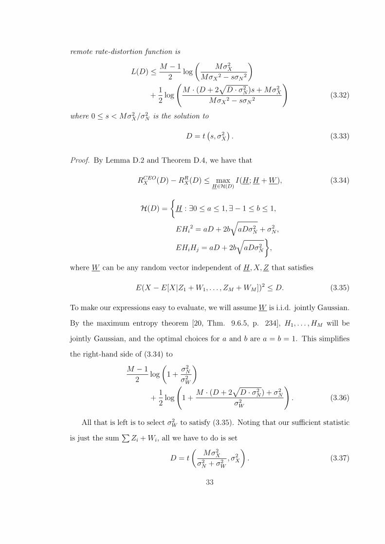
L(D) ≤ M − 1

2log

(Mσ2

X

MσX2 − sσN

2

)

+1

2log

(M · (D + 2

√D · σ2

N)s + Mσ2X

MσX2 − sσN

2

)(3.32)

where 0 ≤ s < Mσ2X/σ2

N is the solution to

D = t(s, σ2

X

). (3.33)

Proof. By Lemma D.2 and Theorem D.4, we have that

RCEOX (D)−RR

X(D) ≤ maxH∈H(D)

I(H; H + W ), (3.34)

H(D) =

{H : ∃0 ≤ a ≤ 1,∃ − 1 ≤ b ≤ 1,

EHi2 = aD + 2b

√aDσ2

N + σ2N ,

EHiHj = aD + 2b√

aDσ2N

},

where W can be any random vector independent of H,X,Z that satisfies

E(X − E[X|Z1 + W1, . . . , ZM + WM ])2 ≤ D. (3.35)

To make our expressions easy to evaluate, we will assume W is i.i.d. jointly Gaussian.

By the maximum entropy theorem [20, Thm. 9.6.5, p. 234], H1, . . . , HM will be

jointly Gaussian, and the optimal choices for a and b are a = b = 1. This simplifies

the right-hand side of (3.34) to

M − 1

2log

(1 +

σ2N

σ2W

)

+1

2log

(1 +

M · (D + 2√

D · σ2N) + σ2

N

σ2W

). (3.36)

All that is left is to select σ2W to satisfy (3.35). Noting that our sufficient statistic

is just the sum∑

Zi + Wi, all we have to do is set

D = t

(Mσ2

X

σ2N + σ2

W

, σ2X

). (3.37)

33

Defining s =Mσ2

X

σ2N+σ2

W<

Mσ2X

σ2N

, solving for σ2W , and substituting it into (3.36) gives us

our bound in (3.32).

3.3.3 Rate Loss Upper Bound vs. Maximum Entropy Upper

Bound

10−5

10−4

10−3

10−2

10−1

100

0

0.5

1

1.5

Difference between R1 (D) and L(D) for BPSK Source, M arbitrary, σ

X2 = 1, σ

N2 = 1

D

nats

log(2)

Figure 3.3. When the curve crosses log(2), the rate loss approach provides a betterbound than the maximum entropy bound for the BPSK source and large enough M .

Instead of computing RRX(D) exactly, we consider approaches to find an upper

bound for it. A maximum entropy bound on RRX(D) results in a bound that is worse

than R1(D) (see Appendix). For this reason, the rate loss approach gives a worse

bound than R1(D) for the Gaussian case, for which the latter is tight. Thus, we move

away from bounds RRX(D) that hold for all possible sources, and consider specializing

34

it to specific sources. To see how good such bounds on RRX(D) need to be, consider

what happens when we subtract (3.32) from (3.29).

R1(D)− L(D) ≥ 1

2log

(σ2

X

D + 2√

D · σ2N + Dl

). (3.38)

Thus, when RRX(D) is smaller than (3.38) for some choice of D, then our second

bound will be strictly better than R1(D). Indeed, this turns out to be true for the

BPSK source (Example 1.3), as we now show.

Consider the following coding strategy for the BPSK source in the remote source

coding setting. First, the encoder averages its observations Zi(k), giving

Z(k) =1

M

M∑i=1

Zi(k) = X(k) +1

M

M∑i=1

Ni(k). (3.39)

Next, we quantize these observations to +σX when Z(k) is positive and to −σX when

it is negative. We call the quantized version Z(k). By the same arguments in Example

1.3, this gives

E(X(k)− Z(k))2 ≤ 4σX2 exp

{−Mσ2

X

2σ2N

}, (3.40)

which we get simply by replacing snr withMσ2

X

σ2N

in the right hand side of (1.7). If

we now apply noiseless source coding to the sequence Z(k), it is clear that R = log 2

is sufficient to reconstruct Z(k) with arbitrarily small error probability as the block

length gets large, and that with small enough error probability, we can approach the

distortion on the right-hand side of (3.40) arbitrarily closely.

For large enough M , the right-hand side of (3.40) can be made arbitrarily small.

Thus, for all δ > 0 and for large enough M , (R,D) = (log 2, δ) is achievable in the

remote source coding problem for the BPSK source. Observing that the difference

curve in (3.38) does not depend on M , it is sufficient to show that for the BPSK

source and for some D > 0, this curve is larger than log 2. This is evident in Figure

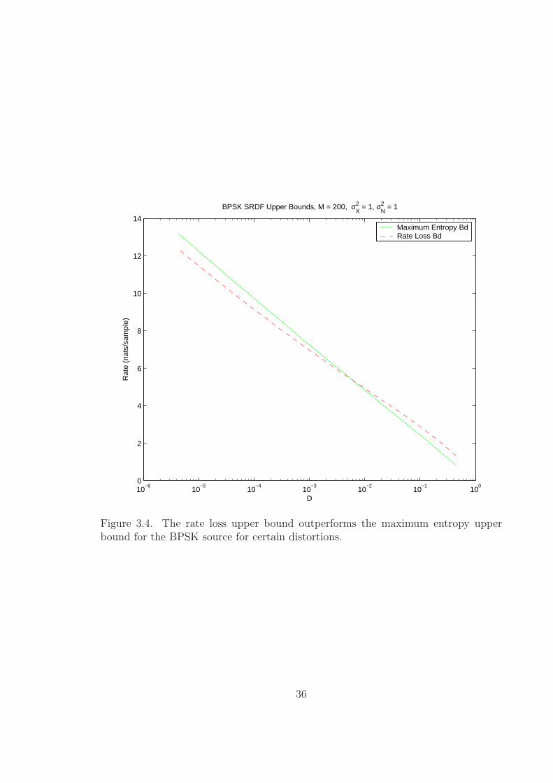
3.3. We also plot an example for the rate loss approach in Figure 3.4

35

10−6

10−5

10−4

10−3

10−2

10−1

100

0

2

4

6

8

10

12

14

BPSK SRDF Upper Bounds, M = 200, σX2 = 1, σ

N2 = 1

D

Rat

e (n

ats/

sam

ple)

Maximum Entropy BdRate Loss Bd

Figure 3.4. The rate loss upper bound outperforms the maximum entropy upperbound for the BPSK source for certain distortions.

36

3.4 Discussion

We presented a lower bound and two upper bounds on the sum-rate-distortion

function for the AWGN CEO problem. The lower bound and the maximum entropy

upper bound are as tight as the gap between the entropy powers and variances found in

their expressions, respectively. To reduce this gap, our rate loss upper bound provides

an improvement on the maximum entropy bound for certain non-Gaussian sources

and certain target distortion values. One disadvantage of this approach is that there

is no simple closed form expression for such a bound, unlike the maximum entropy

bound. One might notice a relationship between the lower bound and maximum

entropy upper bound presented in this chapter with the bounds presented in Chapter

2. In Chapter 4, we explore this relationship in greater detail by considering what

happens as the number of observations gets large in both problems.

37

Chapter 4

Scaling Laws

In this chapter, we examine what happens as the number of observations gets

large in the remote source coding and CEO problems. Recall that in Chapters 2 and

3, we assumed a finite number of observation M and for 1 ≤ i ≤ M ,

Zi(k) = X(k) + Ni(k), k ≥ 1, (4.1)


). In this chapter, we examine what happens as we let M

get large. We will focus exclusively on the case of squared error distortion for both

models. That is, d(x, x) = (x− x)2.

In the next section, we provide definitions and notation that will be useful in

proving our scaling laws. We then present scaling laws for the remote source coding

problem and show that as the number of observations increases, the remote rate-

distortion function converges to the direct rate-distortion function. For the CEO

problem, we find that the sum-rate-distortion function does not converge to the clas-

sical rate-distortion function and that there is, in fact, a penalty. It turns out that

this penalty results in a different scaling behavior for the CEO sum-rate-distortion

function. As a cautionary tale on scaling laws, we consider a coding strategy for the

CEO problem that does not exploit the redundancy among the distributed observa-

38

tions. This “no binning” approach ends up exhibiting the same scaling behavior as

the sum-rate-distortion function in the CEO problem.

4.1 Definitions and Notation

The following definition will allows us to state our scaling law results precisely.

Definition 4.1. Two functions f(D) and g(D) are asymptotically equivalent, de-

noted f(D) ∼ g(D), if there exist positive real numbers K1 and K2 such that

K1 ≤ lim infD→0

f(D)

g(D)≤ lim sup

D→0

f(D)

g(D)≤ K2. (4.2)

For convenience, we will use the following shorthand to refer to scalar sufficient

statistics for X given Z.

Z =1

M

M∑i=1

σ2N

σ2Ni

Zi (4.3)

= X + N , (4.4)

where the harmonic mean σ2N

= 11M

PMi=1

1

σ2Ni

and N = 1M

∑Mi=1

σ2N

σ2Ni

Ni. Note that the

variance of N ∼ N (0, σ2

N/M

). We assume that the harmonic mean σ2

Nstays fixed

as the number of observations M increases. One important case in which this holds

is the equi-variance case in which σ2Ni

= σ2N .

Since the number of observations M is no longer a fixed parameter in our analysis,

we now denote the M -observation remote rate-distortion function and CEO sum-rate-

distortion function as RR,MX (D) and RCEO,M

X (D), respectively. Further, the notation

RR,∞X (D) = limM→∞ RR,M

X (D) and RCEO,∞X (D) = limM→∞ RCEO,M

X (D) will be useful

when stating our scaling laws.

39

4.2 Remote Source Coding Problem

Upper and lower bounds for the remote rate-distortion function with squared error

distortion were given in Corollary 2.5. While one can take the limit of the upper and

lower bounds to derive our scaling law, we will show a slightly stronger result. Before

doing so, we establish the following result for the direct rate-distortion function.

Lemma 4.2. When QX > 0, the direct rate-distortion function behaves as

RX(D) ∼ log1

D. (4.5)

Proof. Recalling the upper and lower bounds to the direct-rate-distortion function in

(1.22), we know that

1

2log

(QX

D

)≤ RX(D) ≤ 1

2log

(σ2

X

D

). (4.6)

From this, we can conclude that

lim supD→0

RX(D)

log 1D

≤ 1, (4.7)

lim infD→0

RX(D)

log 1D

≥ 1. (4.8)

This satisfies the conditions in the definition, so we have established the result.

Theorem 4.3. For the AWGN remote source coding problem with M-observations

and a squared error distortion, the remote rate-distortion function converges to the

direct rate-distortion function as M →∞. That is,

RR,MX (D) → RX(D) (4.9)

as M →∞.

Proof. It is clear that the direct rate-distortion function for X is less than the remote

rate-distortion for X given Z1, . . . , ZM . That is, RX(D) ≤ RR,MX (D) for all M .

40

Thus, all we have to establish is that the remote rate-distortion function for X given

Z1, . . . , ZM converges to a function that is at most the direct rate-distortion function

for X.

By Lemma C.1 and Lemma C.2, we know that it is sufficient to consider the

remote rate-distortion function for X given the sufficient statistic Z defined in (C.2).

By the Cauchy-Schwartz inequality, we know that if E(Z − U)2 = δ, then

δ −√

δσ2

N

M≤ E(X − U)2 ≤ δ +

√δσ2

N

M. (4.10)

Similarly, if E(X − U)2 = δ,

δ −√

δσ2

N

M≤ E(Z − U)2 ≤ δ +

√δσ2

N

M. (4.11)

Thus, by the single-letter characterizations for the direct and remote rate-distortion

functions given in (1.21) and (1.28), respectively, we can conclude that the remote

rate-distortion function for X given Z converges to the direct rate-distortion function

for Z (denoted RMZ

(D)). That is, as M →∞,

∣∣∣RR,MX (D)−RM

Z(D)

∣∣∣ → 0. (4.12)

By the same argument, we know that the remote-rate distortion function for Z given

X (denoted RRZ(D)) converges to the direct rate-distortion function for X. That is,

as M →∞,

RR,M

Z(D) → RX(D). (4.13)

However, we also know that RR,M

Z(D) ≥ RM

Z(D). Thus, we can establish that

RR,MX (D) converges to a function that is at most RX(D), which completes our

proof.

Theorem 4.3 implies that the scaling behavior of the remote source coding problem

is that same as in Lemma 4.2. We summarize this in the following corollary.

41

Corollary 4.4. For the AWGN remote source coding problem with M-observations

and a squared error distortion, the remote rate-distortion function scales as 1D

in the

limit as M →∞. That is,

RR,∞X (D) ∼ log

1

D. (4.14)

4.3 CEO Problem

We now establish a scaling law for the sum-rate-distortion function for the AWGN

CEO problem.

Theorem 4.5. When QX > 0 and the limit of the right-hand side of (3.24) exists as

M →∞,

RCEO,∞X (D) ∼ 1

D. (4.15)

In fact, the following upper and lower bounds hold.

1

2log

(QX

D

)+

σ2N

2

(1

D− J(X)

)

≤ RCEO,∞X (D) ≤

1

2log

(σ2

X

D

)+

σ2N

2

(1

D− 1

σ2X

). (4.16)

Proof. If we can establish (4.16), the scaling law result follows immediately since

lim infD→0

DRCEO,∞X (D) = lim sup

D→0DRCEO,∞

X (D) =σ2

N

2. (4.17)

Taking the limit in (3.24) as M →∞ gives

RCEO,∞X (D) ≥ log

(QX

D

)+

σ2N

2

(1

D− J(X)

), (4.18)

Likewise, we can take the as M →∞ for the upper bound given in (3.28) to get

RCEO,∞X (D) ≤ 1

2log

(σ2

X

D

)+

σ2N

2

(1

D− 1

σ2X

). (4.19)

Thus, we have shown the desired results.

42

Clearly, the above result holds for a Gaussian source. However, we are interested

in finding non-Gaussian sources for which we know this scaling behavior holds. The

following examples show it holds for a Laplacian source as well as a logistic source.

Example 4.6. Consider a data source with a Laplacian distribution. That is,

f(x) =1√2σX

e−√

2|x|σX .

For this data source, the Fisher information is

J(X) =2

σ2X

and the differential entropy is

H(X) =1

2log 2e2σ2

X .

Thus, for this case, the limit exists for the lower bound in (3.24) and is

RCEO,∞X (D) ≥ 1

2log

(eσ2

X

πD

)+

σ2N

2

(1

D− 2

σ2X

), (4.20)

where the inequality follows from (1.22). Thus, we can conclude that for the Laplacian

source, RCEO,∞X (D) ∼ 1

D. The gap between the direct and CEO sum-rate-distortion

function is shown in Figure 4.1.

Example 4.7. Consider a data source with a Logistic distribution. That is,

f(x) =e−

xβ

β(1 + e−

xβ

)2 .

For this data source, the Fisher information is

J(X) =1

3β2,

the entropy power is [20, p. 487]

QX =e3β2

2π,

43

and the variance is

σ2X =

π2β2

3.

Thus, for this case, the limit exists for the lower bound in (3.24), so we can conclude

that for the Logistic source, RCEO,∞X (D) ∼ 1

D. The gap between the direct and CEO

sum-rate-distortion function is shown in Figure 4.2. Notice that the gap is even

smaller than in Example 4.6.

0 0.1 0.2 0.3 0.4 0.5 0.6 0.7 0.8 0.9 10

10

20

30

40

50

60

Scaling Law Behavior for Laplacian Source with σX2 = 1, σ

N2 = 1

Rat

e (n

ats/

sam

ple)

Distortion

CEO Upper Bound CEO Lower Bound Classical Upper BoundClassical Lower Bound

Figure 4.1. Scaling behavior for Laplacian source in AWGN CEO Problem

4.4 No Binning

As a cautionary tale about the utility of scaling laws, we consider a coding strategy

in which encoders do not exploit the correlation with observations at other encoders.

44

0 0.1 0.2 0.3 0.4 0.5 0.6 0.7 0.8 0.9 10

10

20

30

40

50

60

Scaling Law Behavior for Logistic Source with σX2 = 1, σ

N2 = 1

Rat

e (n

ats/

sam

ple)

Distortion

CEO Upper Bound CEO Lower Bound Classical Upper BoundClassical Lower Bound

Figure 4.2. Scaling behavior for Logistic source in AWGN CEO Problem

45

We call this approach the “no binning” strategy and denote the minimal achievable

sum-rate-distortion pairs by the function RNB,MX (D) for M -observations. It turns

out that for certain cases, the scaling behavior remains the same as the sum-rate-

distortion function. We consider two such cases. The first is for the case of the

quadratic AWGN CEO problem, which we have already considered. The second is

based on a different CEO problem introduced by Wagner and Anantharam [11], [25].

The strategies that we consider are closely related to special cases of robust coding

strategies considered by Chen et. al. [26].

4.4.1 Quadratic AWGN CEO Problem

Our first case involves the quadratic AWGN CEO problem. That is, the AWGN

CEO problem with a squared error distortion. The coding strategy simply involves

vector quantizing the observations and then performing an estimate at the decoder.

This is similar to the coding strategy we used in our upper bound for the AWGN

CEO sum-rate-distortion function, except now we have removed the binning stage.

Theorem 4.8. When QX > 0 and the limit of the right-hand side of (3.24) exists as

M →∞, then the minimal sum-rate distortion pairs achievable by this coding strategy

is

RNB,∞X (D) ∼ 1

D. (4.21)

Proof. The lower bound follows immediately from the previous lower bound in (4.18).

Thus, it is simply a matter of providing an upper bound on the performance of codes

with our structure. For such codes, we can show that random quantization arguments

give

R =M∑i=1

I(Zi; Ui), (4.22)

D = E(X − E[X|U1, . . . , UM ])2 (4.23)

46

as an achievable sum-rate distortion pair for auxiliary random variables Ui satis-

fying Ui ↔ Zi ↔ X, U{i}c ,Z{i}c . Defining Ui = Zi + Wi where the Wi are inde-

pendent Gaussian random variables and applying the maximum entropy bound for

H(Z1, . . . , ZM) [20, Thm. 9.6.5, p. 234], we get that

RNB,MX (D) ≤M

2log

(1 +

σ2X

D− 1

M

)

+M

2log

Mσ2

X

Mσ2X −

(σ2

X

D− 1

)σ2

N

(4.24)

Taking the limit as M →∞ gives

RNB,∞X (D) ≤ σ2

X + σ2N

2

(1

D− 1

σ2X

). (4.25)

Thus, we have that

σ2N

2≤ lim inf

D→0DRNB,∞

X (D)

≤ lim supD→0

DRNB,∞X (D) ≤ σ2

X + σ2N

2, (4.26)

and we have proved the desired result.

While the above shows that we can achieve the same scaling behavior, the per-

formance loss can still be large in some instances. The following result bounds the

performance loss.

Theorem 4.9. Let DNB,∞X (R) denote the inverse function of RNB,∞

X (D) and likewise

for DCEO,∞X (R). Then, as R →∞,

10 log10 DNB,∞X − 10 log10 DCEO,∞

X

≤ 10 log10

(1 +

σ2X

σ2N

)dB. (4.27)

Proof. We can bound the performance loss for this robustness by rearranging (4.25)

47

and (4.16) to get, for large enough R,

10 log10 DNB,∞X (R)− 10 log10 DCEO,∞

X (R)

≤ 10 log10

(1 +

σ2X

σ2N

)+ 10 log10

R + J(X)

(σ2

N

2

)

R + 1σ2

X

(σ2

X+σ2N

2

) dB. (4.28)

Thus, at high rates (R →∞), the performance loss is upper bounded by

10 log10

(1 +

σ2X

σ2N

)dB. (4.29)

This completes the result

For Gaussian sources, the above bound is valid for any choice of R. A summary

for the performance loss for different SNR inputs at each sensor is given in Table 4.1.

SNR (dB) Loss (dB)10 10.415 6.191 3.540 3.01-1 2.53-5 1.19-10 0.41

Table 4.1. Performance loss for a “no binning” coding strategy in the quadraticAWGN CEO problem.

4.4.2 Binary Erasure

For our second example, we consider a different CEO problem introduced by

Wagner and Anantharam [11], [25]. In this problem, the source X = ±1, each with

probability 1/2. Each of the encoders views the output of X through an independent

binary erasure channel with crossover probability ε. Thus, Zi ∈ {−1, 0, 1}. The

48

distortion of interest to the CEO is

d(x, x) =

K À 1, x 6= x, x 6= 0

1 x = 0

0 x = x

.

It turns out that as K gets large, the asymptotic sum-rate-distortion function for this

binary erasure CEO problem is [25]

RCEO,∞BE (D) = (1−D) log 2 + log

(1

D

)log

(1

1− ε

). (4.30)

Theorem 4.10. For the binary erasure the sum-rate distortion pairs achievable by a

“no binning” strategy have the property

RNB,∞BE (D) ∼ RCEO,∞

BE (D). (4.31)

Proof. Since RNB,∞BE (D) ≥ RCEO,∞

BE (D), the lower bound is clear. By random quanti-

zation arguments, we can show that for an appropriately chosen f ,

R =M∑i=1

I(Zi; Ui), (4.32)

D = Pr (f(U1, . . . , UM) = 0) (4.33)

is an achievable sum-rate distortion pair for auxiliary random variables Ui satisfying

Ui ↔ Zi ↔ X,U{i}c ,Z{i}c . Defining Ui = Zi · Qi where Qi ∈ {0, 1} are Bernoulli-q

random variables, then D is just simply the probability that all the Ui are 0, which

is just

D = (1− (1− ε)(1− q))M . (4.34)

Taking the limit as M →∞ gives

RNB,∞X (D) ≤ log

(1

D

)+ log

(1

D

)log

(1

1− ε

). (4.35)

Thus, we have that

lim supD→0

RNB,∞X (D)

RCEO,∞BE (D)

≤ 1 +

(log

(1

1− ε

))−1

, (4.36)

and we have proved the desired result.

49

4.5 Discussion

In this chapter, we have presented bounds for the remote rate-distortion function

and CEO sum-rate-distortion function as the number of observations increases. While

the remote rate-distortion function converges to the direct rate-distortion function,

there is still a rate loss asymptotically in the AWGN CEO problem. It turns out that

even significantly suboptimal coding strategies can yield the same scaling behavior,

leading one to question the sufficiency of scaling laws to characterize tradeoffs in such

problems.

50

Chapter 5

Conclusion and Future Work

In 1959, Claude Shannon characterized the direct rate-distortion function and gave

closed-form upper and lower bounds to it [1]. In this thesis, we presented extensions

of these bounds to remote source coding problems. In particular, we considered the

case in which the observations were corrupted by additive noise and the distortion

was squared error.

We first gave bounds for the case of centralized encoding and decoding. Like Shan-

non’s bounds for squared error distortion, the upper and lower bounds had similar

forms with the upper bound matching the Gaussian remote rate-distortion function.

The lower bound met the upper bound for the Gaussian source and entropy powers

took the place of variances for non-Gaussian sources. Unlike previously known lower

bounds for this problem, the lower bound in this problem was easier to compute for

non-Gaussian sources.

We then gave bounds for the case of distributed encoding and centralized decoding,

the so-called CEO problem. The lower bound appears to be the first non-trivial lower

bound to the sum-rate-distortion function for AWGN CEO problems. We also consid-

ered two upper bounds for the sum-rate-distortion function. The second, while not as

51

elegant as the first, proved to be more useful for certain non-Gaussian sources. Again,

for the sum-rate-distortion function, the upper bounds and lower bounds matched for

the case of the Gaussian source.

Using these bounds, we derived scaling laws for these problems. We found that

while the case of centralized encoding and decoding could overcome the noise and con-

verge to the direct rate-distortion function in the limit as the number of observations

increases, the CEO sum-rate-distortion function converges to a larger function that

has a different scaling behavior at low distortions. We also noted that one can still

maintain this scaling behavior even none of the encoders take advantage of correlation

among the different observations in the distributed coding scheme.

The results presented here pave the way for new research directions. One would

be to consider the case in which the source or noise processes have memory. One can

also consider how to handle different types of noise distributions as well as different

distortions. Further, the bounds presented about the CEO problem appear to are

related to the µ-sums problem considered by Wagner et. al. in [25]. Using the results

given here, one might be able to provide similar results for the case of Gaussian

mixtures.

52

References

[1] C. Shannon, “Coding theorems for a discrete source with a fidelity criterion,” IRE ConventionRec., vol. 7, p. 142, 1959.

[2] T. Berger and J. Gibson, “Lossy source coding,” IEEE Transactions on Information Theory,vol. 44, no. 6, p. 2693, 1998.

[3] R. Blahut, “Computation of channel capacity and rate-distortion functions,” IEEE Transactionson Information Theory, vol. 18, p. 460, 1972.

[4] S. Arimoto, “An algorithm for calculating the capacity and rate-distortion functions,” IEEETransactions on Information Theory, vol. 18, p. 14, 1972.

[5] K. Rose, “A mapping approach to rate-distortion computation and analysis,” IEEE Transac-tions on Information Theory, vol. 40, p. 1939, 1994.

[6] R. Dobrushin and B. Tsybakov, “Information transmission with additional noise,” IEEE Trans-actions on Information Theory, vol. 8, p. 293, 1962.

[7] J. Wolf and J. Ziv, “Transmission of noisy information to a noisy receiver with minimumdistortion,” IEEE Transactions on Information Theory, vol. 16, pp. 406–411, 1970.

[8] T. Berger, Rate Distortion Theory: A Mathematical Basis for Data Compression, ser. Informa-tion and System Sciences Series. Englewood Cliffs, NJ, USA: Prentice-Hall, 1971.

[9] ——, “Multiterminal source coding,” in Lecture Notes presented at CISM Summer School onthe Information Theory Approach to Communications, 1977.

[10] S. Tung, “Multiterminal source coding,” Ph.D. dissertation, Cornell University, 1977.[11] A. Wagner and V. Anantharam, “An improved outer bound for the multiterminal source coding

problem,” in International Symposium on Information Theory, 2005.[12] A. B. Wagner, “Methods of offline distributed detection: Interacting particle models and

information-theoretic limits,” Ph.D. dissertation, University of California, Berkeley, 2005.[13] T. Berger, Z. Zhang, and H. Viswanathan, “The CEO problem,” IEEE Transactions on Infor-

mation Theory, vol. 42, pp. 887–902, May 1996.[14] H. Viswanathan and T. Berger, “The quadratic Gaussian CEO problem,” IEEE Transactions

on Information Theory, vol. 43, pp. 1549–1559, 1997.[15] V. Prabhakaran, D. Tse, and K. Ramchandran, “Rate region of the quadratic Gaussian CEO

problem,” in Proceedings of ISIT, 2004.[16] Y. Oohama, “Rate-distortion theory for Gaussian multiterminal source coding systems with

several side informations at the decoder,” IEEE Transactions on Information Theory, vol. 51,pp. 2577–2593, 2005.

[17] D. Guo, S. Shamai, and S. Verdu, “Mutual information and minimum mean-square error inGaussian channels,” IEEE Transactions on Information Theory, vol. 51, pp. 1261–1282, 2005.

[18] M. Pinsker, Information and Information Stability of Random Variables and Processes. SanFrancisco: Holden-Day, 1964, translated by A. Feinstein.

[19] A. Wyner, “The rate-distortion function for source coding with side information at the decoderII: General sources,” Information and Control, vol. 19, pp. 60–80, 1978.

[20] T. Cover and J. Thomas, Elements of Information Theory. John Wiley and Sons, 1991.[21] M. Gastpar, “A lower bound to the AWGN remote rate-distortion function,” in 2005 Statistical

Signal Processing Workshop, Bordeaux, France, 2005.[22] K. B. Housewright, “Source coding studies for multiterminal systems,” Ph.D. dissertation,

University of California, Los Angeles, 1977.[23] J. Chen, X. Zhang, T. Berger, and S. B. Wicker, “An upper bound on the sum-rate distortion

function and its corresponding rate allocation schemes for the CEO problem,” IEEE Journalon Selected Areas in Communications: Special Issue on Sensor Networks, pp. 1–10, 2003.

53

[24] Y. Oohama, “Multiterminal source coding for correlated memoryless Gaussian sources withseveral side informations at the decoder,” in ITW, 1999.

[25] A. B. Wagner, S. Tavildar, and P. Viswanath, “The rate region of the quadratic Gaussiantwo-terminal source-coding problem,” 2005. [Online]. Available: http://www.citebase.org/cgi-bin/citations?id=oai:arXiv.org:cs/0510095

[26] J. Chen and T. Berger, “Robust distributed source coding,” IEEE Transactions on InformationTheory, submitted.

[27] N. Blachman, “The convolution inequality for entropy powers,” IEEE Transactions on Infor-mation Theory, vol. 11, p. 267, 1965.

[28] H. V. Poor, Introduction to Signal Detection and Estimation, ser. Texts in Electrical Engineer-ing. New York: Springer-Verlag, 1994.

[29] M. Costa, “A new entropy power inequality,” IEEE Transactions on Information Theory,vol. 31, p. 751, 1985.

[30] R. Durrett, Probability: Theory and Examples, 3rd ed, ser. Information and System SciencesSeries. Duxbury, 2004.

[31] H. Witsenhausen, “On the structure of real-time source coders,” Bell System Technical Journal,vol. 58, no. 6, pp. 1437–1451, 1979.

[32] R. Zamir, “The rate loss in the Wyner-Ziv problem,” IEEE Transactions on Information The-ory, vol. 42, pp. 2073–2084, Nov. 1996.

54

Appendix A

Lower Bounds on MMSE

In this appendix, we show that for a large class of sources corrupted by additiveGaussian noise have mean squared error decaying as Θ

(1

snr

)where snr is the signal-

to-noise ratio of the source viewed in additive noise. The main conditions on thesources are that they have finite variance and are continuous.

Although we specialize our proofs to cases in which the noise is additive Gaus-sian, the same arguments work for any additive noise N with variance σ2 for which12log σ2−h(N) = K, where K is a constant that does not depend σ2. The only thing

that changes is the scaling constant. Table A.1 lists examples of sources for whichthis is true.

Distribution Density Variance Entropy

Gaussian(0, σ2) f(x) = 1√2πσ2

e−x2/2σ2σ2 1

2log(2πeσ2)

Laplacian(λ) f(x) = λ2e−λ|x| σ2 = 2

λ212log(2e2σ2)

Uniform(−a, a) f(x) = 12a

1{x∈[−a,a]} σ2 = 13a2 1

2log(12σ2)

Two Pulse(c, ε) f(x) = 14cε

1{x∈[−c(1+ε),−c(1−ε)]∪[c(1−ε),c(1+ε)]}

σ2 = c2(1 + ε2/3) 12log

(16ε2σ2

1+ε2/3

)

Table A.1. Distributions and their differential entropies.

In the sequel, we denote our source as the random variable X with variance σ2X .

X is corrupted by independent additive noise N with variance σ2X/s. This gives

the signal-to-noise ratio s. We are interested in the performance of the estimatorE[X|X + N ] as a function of s for fixed σ2

X .

Lemma A.1. Define m(s) = E(X − E[X|X + N ])2. Then

m(s) ≤ σ2X

s + 1. (A.1)

Proof. Using the linear estimator X =σ2

X

σ2X+σ2

X/s(X +N), we get a mean squared error

55

upper bound of

E(X − E[X|X + N ])2 ≤ E(X − X)2 =σ2

X

s + 1. (A.2)

We have now established that the decay in MMSE is always at least as fast ass−1. In fact, the bound in Lemma A.1 is tight for the Gaussian case. However, weare still left with the following question. Are there sources for which this decay isfaster than s−1? The answer to this question is yes. For discrete sources, the MMSEdecays exponentially in s.

We now modify the question. Are there any continuous sources for which thedecay is faster than s−1? Consider the one in Figure A.1. While it is not discrete,its probability is concentrated around two regions. Despite this fact, it will turn outthat even the source in Figure A.1 decays as s−1. The key observation is to note thatH(X), the differential entropy of X, is finite.

6fX (x)

Figure A.1. Example of a source that decays as s−1.

The following lemma will help us obtain this result.

Lemma A.2. Let QX , QN , and QX+N be the normalized (by 2πe) entropy powers ofX, N , and X + N , respectively. Then

E(X − E[X|X + N ])2 ≥ QXQN

QX+N

. (A.3)

Proof. The result is related to a derivation of the Shannon lower bound for squarederror distortion (see e.g. [8]). That is,

I(X; X + N) = H(X)−H(X|X + N) (A.4)

= H(X)−H(X − E[X|X + N ]|X + N) (A.5)

≥ H(X)−H(X − E[X|X + N ]) (A.6)

≥ H(X)− 1

2log

(2πeE(X − E[X|X + N ])2

). (A.7)

However, since I(X; X + N) = H(X + N) − H(N), we can rearrange and recollectterms in (A.7) to conclude the result.

56

Theorem A.3. If H(X) > −∞, then for N ∼ N (0, σ2X/s) independent of X, then

m(s) = E(X − E[X|X + N ])2 = Θ(s−1

). (A.8)

Further,

m(s) ≥ QX

s + 1. (A.9)

Proof. We already established the upper bound in Lemma A.1. Further, by LemmaA.2, we know that

≥ QXQN

QX+N

. (A.10)

Since N is Gaussian, its normalized entropy power QN = σ2X/s. Further, by the

maximum entropy theorem under second moment constraints, QX+N ≤ σ2X + σ2

X/s.With these facts, we can conclude the lower bound in (A.9).

One can generalize the result easily to the following case.

Corollary A.4. If H(X|U) > −∞, then for N ∼ N (0, σ2x/s) independent of X, U ,

m(s) = E(X − E[X|U,X + N ])2 = Θ(s−1

). (A.11)

Further,

m(s) ≥1

2πeexp{2H(X|U)}

s + 1. (A.12)

Proof. The upper bound in Lemma A.1 continues to hold. We now have the bounds

H(X|U)− 1

2log(2πem(s)) ≤ I(X; X + N |U) ≤ I(X, U ; X + N). (A.13)

where the lower bound follows as before. We get the upper bound by writing

I(X, U ; X + N) ≤ H(X + N)−H(X + N |X, U) (A.14)

= H(X + N)−H(N |X, U) (A.15)

= H(X + N)−H(N) (A.16)

≤ 1

2log(1 + s). (A.17)

Now, by the same arguments given in Theorem A.3, we can conclude (A.12) andthereby (A.11).

Suppose now we consider a source that is either discrete or continuous conditionedon a random variable T . In particular, suppose a source X is 0 when T = d and Xhas a pdf like the one in Figure A.1 when T = c. Can this scale faster than s−1? Theanswer again turns out to be no.

57

Corollary A.5. If H(X|T = c) > −∞ and V ar(X|T = c) = ασ2X for some α < ∞,

then for N ∼ N (0, σ2X/s) independent of X, T ,

m(s) = E(X − E[X|X + N ])2 = Θ(s−1

). (A.18)

Further,

m(s) ≥ P (T = c)1

2πeαexp{2H(X|T = c)}

s + 1. (A.19)

Proof. This follows immediately from Theorem A.3 by conditioning on the event{T = c}.

58

Appendix B

Unified Entropy Power Inequality

We prove an inequality that specializes to the entropy power inequality in one case,Costa’s entropy power inequality [29] in a second, and an entropy power inequalityused by Oohama to prove a converse to the sum-rate-distortion function for GaussianCEO problem in a third [16]. The generalization allows us to generalize his converseapproach to give lower bounds to the sum-rate-distortion function for non-Gaussiansources in the AWGN CEO problem (see Chapter 3). It is also useful for new lowerbounds for the remote rate-distortion function (see Chapter 2).

In the next section, we state the main result and give some interpretations ofit. The remainder of this appendix is devoted to the proof. Our goal is to define afunction on the positive reals that is the ratio between the right- and left-hand sideof our inequality at 0 and show that it increases monotonically to 1, as in Figure B.1.To do this, we find derivatives of the differential entropies in our expressions and thenestablish inequalities about these derivatives. We then applies these inequalities onthe function we defined and show that it has a positive derivative at all points.

B.1 Main Result

In this section, we state the main result. We also briefly describe how one can getother inequalities in this case.

Theorem B.1. X and N are independent random vectors in Rn. Let Z = X + Nand require that X ↔ Z ↔ W , where W is some auxiliary random variable. Then

e2n

H(Z)

e2n

I(X;W )≥ e

2n

H(X)

e2n

I(Z;W )+ e

2n

H(N). (B.1)

The original entropy power inequality follows when Z is independent of W . WhenN is Gaussian and W = Z + N2, where N2 is additional Gaussian noise, we get

59

Costa’s entropy power inequality [29]. Note that we can rewrite (B.1) as

e2n

H(X|W ) ≥ e2n

H(Z|W )

(e

2n

I(N;Z))2 +

e2n

H(N)

e2n

I(N;Z). (B.2)

For the special case when X and N are Gaussian, this becomes Oohama’s entropypower inequality [16, eq. (48)]. It can be thought of as a “reverse” entropy powerinequality in the sense that one of the addends in the traditional entropy powerinequality is on the left-hand side of this inequality. Note that unlike his case, whichfollows from the relationship between independence and uncorrelatedness for Gaussianrandom variables, our result shows that the inequality holds simply by Bayes’ rule.Another way of writing the inequality is

1

nI(X; W ) ≤ 1

nI(X;Z)− 1

2log

(e−

2n

I(N;Z) + e−2n

I(X;Z)e2I(Z;W )

e−2n

I(X;Z)e2n

I(Z;W )

). (B.3)

This gives a tighter bound than the data processing inequality under additional struc-ture assumptions.

B.2 Definitions and Notation

The proof follows along the lines of Blachman’s proof [27] of the original entropypower inequality, except we treat the vector case directly. Before moving on to theproof, we introduce Fisher information and provide a few basic properties of it.

Definition B.2. Let X be a random vector in Rn. If X has a pdf f(x), the trace ofthe Fisher information matrix of X is

J(X) =

∫

Rn

‖∇f(x)‖2

f(x)dx. (B.4)

This definition is based on the case in which one is interested in estimating means,so it differs slightly from [28]. The relationship is described in [20, p. 194]

Definition B.3. Let X be a random vector in Rn and W a random variable. If Xhas a conditional pdf f(x|w), the conditional Fisher information of X given W is

J(X|W ) =

∫µ(dw)

∫

Rn

‖∇xf(x|w)‖2

f(x|w)dx. (B.5)

One might recall de Bruijn’s identity [20, Theorem 16.6.2]. The following is astatement of the vector version.

Lemma B.4. Let X be a random vector in Rn. We denote Xt = X+√

tV, where Vis a standard normal Gaussian random vector. We denote the pdf of Xt with ft(x).Then

d

dtH(Xt) =

1

2J(Xt). (B.6)

60

Proof. See [29].

The following is a conditional version of the identity.

Lemma B.5. Let X be a random vector in Rn. We denote Xt = X +√

tV, whereV is a standard normal Gaussian random vector independent of (X, W ). We denotethe pdf of Xt with ft(x). Then,

d

dtH(Xt|W ) =

1

2J(Xt|W ). (B.7)

Proof. Smoothing the distribution of X by a Gaussian√

tV is equivalent to smoothingthe conditional distribution of X on any realization W = w by

√tV. A formal argu-

ment requires applying Fubini’s theorem and the uniqueness of the Radon-Nikodymderivative [30], but the observation should be intuitively obvious. From this fact, wefind that, for U independent of (X,V,W ),

0 ≤ H(Xt +√

hU|W = w)−H(Xt|W = w) ≤ 1

2log

(t + h

t

)≤ h

2t, (B.8)

where the first inequality follows from the non-negativity of mutual information,the second from the data processing inequality, and the third from the inequalitylog(1 + x) ≤ x. Thus,

0 ≤ H(Xt +√

hU|W = w)−H(Xt|W = w)

h≤ 1

2t, (B.9)

so by bounded convergence, we can swap the derivative and expectation over W toconclude the result.

Lemma B.6. Let X be a random vector in Rn. We denote Xt = X +√

tV, whereV is a standard Gaussian random vector independent of (X, W ). Then,

J(Xt|W ) ≥ J(Xt). (B.10)

Proof. Let U be a standard Gaussian random vector independent of (X,V,W ).Then, by the data processing inequality,

I(Xt; W ) ≥ I(Xt +√

hU; W ). (B.11)

Thus, for all h > 0,

0 ≥ I(Xt +√

hU; W )− I(Xt; W )

h(B.12)

=H(Xt +

√hU)−H(Xt)

h− H(Xt +

√hU|W )−H(Xt|W )

h. (B.13)

Letting h → 0 and applying Lemmas B.4 and B.5 gives the desired result.

61

B.3 Fisher Information Inequalities

We now consider Fisher information inequalities that will allow us to show thata function we define momentarily has a positive derivative at all points. The follow-ing inequality is sufficient to prove the classical entropy power inequality shown byBlachman [27].

Lemma B.7. Let X,N be independent random vectors and Z = X + N with differ-entiable, nowhere vanishing densities fX(·), fN(·), and fZ(·). Then

1

J(Z)≥ 1

J(X)+

1

J(N)(B.14)

Proof. See Blachman [27] for the scalar version. The vector proof is the same exceptderivatives are replaced by gradients.

For our generalization of the entropy power inequality, we require an additionalinequality that we now state.

Lemma B.8. Let X,N be independent random vectors and Z = X+N with differen-tiable, nowhere vanishing densities fX(·), fN(·), and fZ(·). If X ↔ Z ↔ W for somerandom variable W and fX|W (·|w) fZ|W (·|w) are differentiable, nowhere vanishingconditional densities, then

J(X|W )− J(X) ≤ J(N) (J(Z|W )− J(Z))

J(Z|W )− J(Z) + J(N). (B.15)

Note that when J(X|W ) > J(X) and J(Z|W ) > J(Z), we can rewrite (B.15) as

1

J(X|W )− J(X)≥ 1

J(Z|W )− J(Z)+

1

J(N)(B.16)

Proof. We follow a similar argument in Blachman [27] for Lemma B.7. By a straight-forward application of Bayes’ rule, we can write

fX|W (x|w) =

∫

Rn

fX(x)fN(x− z)

fZ(z)fZ|W (z|w)dz. (B.17)

= fX(x)

∫

Rn

fN(x− z)

fZ(z)fZ|W (z|w)dz. (B.18)

Since we have assumed differentiability, we can write the gradient as

∇fX|W (x|w) = (∇fX(x))

∫

Rn

fN(x− z)

fZ(z)fZ|W (z|w)dz

+ fX(x)

∫

Rn

fZ|W (z|w)fN(x− z)

fZ(z)

∇fN(x− z)

fN(x− z)dz. (B.19)

62

Dividing (B.19) by (B.18) gives

∇fX|W (x|w)

fX|W (x|w)=∇fX(x)

fX(x)+

∫

Rn

fZ|W (z|w)fN(x− z)fX(x)

fZ(z)fX|W (x|w)

∇fN(x− z)

fN(x− z)dz. (B.20)

= E

[∇fX(X)

fX(X)+∇fN(N)

fN(N)

∣∣∣∣X = x,W = w

]. (B.21)

Observing that the integral in (B.18) is simply a convolution, the same argumentsgive us

∇fX|W (x|w)

fX|W (x|w)= E

[∇f(X)

fX(X)+∇fZ|W (Z|W )

fZ|W (Z|W )− ∇fZ(Z)

fZ(Z)

∣∣∣∣X = x,W = w

]. (B.22)

We can combine (B.21) and (B.22) by the linearity of expectations to give

(a + b)∇fX|W (x|w)

fX|W (x|w)=E

[(a + b)

∇f(X)

fX(X)+ a

∇fN(N)

fN(N)

+b

(∇fZ|W (Z|W )


fZ(Z)

)∣∣∣∣X = x,W = w

]. (B.23)

Conditional Jensen’s inequality implies that

(a + b)2

∥∥∥∥∇fX|W (x|w)

fX|W (x|w)

∥∥∥∥2

≤

E

[∥∥∥∥(a + b)∇f(X)

fX(X)+ a

∇fN(N)

fN(N)+ b

(∇fZ|W (Z|W )


fZ(Z)

)∥∥∥∥2∣∣∣∣∣

X = x,W = w

].

(B.24)

It is straightforward to check that

E

[⟨∇fZ|W (Z|W )

fZ|W (Z|W ),∇fZ(Z)

fZ(Z)

⟩]= J(Z),

E

[⟨∇fZ|W (Z|W )

fZ|W (Z|W ),∇fN(N)

fN(N)

⟩]= E

[⟨∇fZ(Z)

fZ(Z),∇fN(N)

fN(N)

⟩],

E

[⟨∇fZ|W (Z|W )

fZ|W (Z|W ),∇f(X)

fX(X)

⟩]= E

[⟨∇fZ(Z)

fZ(Z),∇f(X)

fX(X)

⟩].

Taking the expectation of (B.23) and knowing these facts, we get

(a + b)2J(X|W ) ≤ (a + b)2J(X) + a2J(N) + b2 (J(Z|W )− J(Z)) . (B.25)

We can rewrite this as

J(X|W )− J(X) ≤ a2J(N) + b2 (J(Z|W )− J(Z))

(a + b)2. (B.26)

When J(Z|W )− J(Z) = 0, we show that (B.15) holds by making b arbitrarily large.When J(Z|W ) − J(Z) > 0, we simply set a = 1

J(N)and b = 1

J(Z|W )−J(Z)to give

(B.15).

63

6

-

s(t)

1

s(0)

Figure B.1. Desired behavior of s(t)

B.4 Gaussian Smoothing

To finish the proof, the idea is that since we know the result is Gaussian, wesmooth all the distributions until they approach a Gaussian, and then show that thissmoothing can only increase the ratio. We smooth X by a an iid Gaussian vectorU ∼ N (0, f(t)I) independent of (X,N,W ) and smooth N by an iid Gaussian vectorV ∼ N (0, g(t)I) independent of (X,N,W,U), where I is the identity matrix. Thisinduces smoothing on Z by an iid Gaussian vector of variance h(t) = f(t) + g(t).We denote the smoothed random variables as Xf = X + U, Ng = N + V, andZh = Z + U + V, respectively. This will also result in smoothed the conditionaldistributions. We now define

s(t) =e2/n(H(Xf )−I(Zh;W )) + e2/nH(Ng)

e2/n(H(Zh)−I(Xf ;W ))(B.27)

We let f(0) = g(0) = h(0) = 0. Thus, our goal is to show that s(0) ≤ 1, which we do

by showing that for f ′(t) = e2/n(H(Xf )−I(Zh;W )) and g′(t) = e2/nH(Ng), s′(t) ≥ 0 andthen showing that either s(+∞) = 1 or s(0) = 1 trivially.

Lemma B.9. Let f(0) = g(0) = 0, f ′(t) = e2/n(H(Xf )−I(Zh;W )), and g′(t) = e2/nH(Ng).Then, for all t,

s′(t) ≥ 0 (B.28)

Proof. Taking the derivative,

e2/n(H(Zh)−I(Xf ;W ))s′(t) =e2/n(H(Xf )−I(Zh;W )) (f ′(t)J(Xf ) + h′(t)(J(Zh|W )− J(Zh))))

64

+ e2/nH(Ng)g′(t)J(Ng)

−[e2/n(H(Xf )−I(Zh;W )) + e2/nH(Ng)

]

· (h′(t)J(Zh) + f ′(t)(J(Xf |W )− J(Xf ))). (B.29)

Applying Lemmas B.7 and B.8 to the final term and factoring yields

e2/n(H(Zh)−I(Xf ;W ))s′(t) ≥(f ′(t)J(Xf )− g′(t)J(Ng))

(e2/n(H(Xf )−I(Zh;W ))J(Xf )− e2/nH(Ng)J(Ng)

)

J(Xf ) + J(Ng)

+ (f ′(t) + g′(t))(J(Zh|W )− J(Zh))

2e2/n(H(Xf )−I(Zh;W ))

J(Zh|W )− J(Zh) + J(Ng)

+(e2/n(H(Xf )−I(Zh;W ))g′(t)− e2/nH(Ng)f ′(t)

) J(Ng)

J(Zh|W )− J(Zh) + J(Ng)(B.30)

Setting f ′(t) = e2/n(H(Xf )−I(Zh;W )) and g′(t) = e2/nH(Ng), this simplifies to

e2/n(H(Zh)−I(Xf ;W ))s′(t) ≥

(e2/n(H(Xf )−I(Zh;W ))J(Xf )− e2/nH(Ng)J(Ng)

)2

J(Xf ) + J(Ng)+

(e2/n(H(Xf )−I(Zh;W )) + e2/nH(Ng)

) (J(Zh|W )− J(Zh))2e2/n(H(Xf )−I(Zh;W ))

J(Zh|W )− J(Zh) + J(Ng)≥ 0.

(B.31)

This establishes the result.

Proof of Theorem B.1. With Lemma B.9, all that is left is to establish that s(+∞) =1 and when s′(t) = 0 for all t, then s(0) = 1 trivially. We establish the latter casefirst. The cases in which s′(t) = 0 for all t happen when any differential entropy ormutual information is infinite. Note that when any of H(N), H(X), and H(Z) areinfinite, the inequality is satisfied automatically if one appeals to the non-negativityof mutual information (H(Z) ≥ H(N) H(Z) ≥ H(X)) and the data processinginequality (I(X; W ) ≤ I(X;Z) and I(X; W ) ≤ I(Z; W )). Further, our inequalityis an immediate consequence of the data processing inequality when I(Z; W ) = ∞.Thus, we only need to consider the case in which these terms are finite.

Since f ′(t) > 0 and increasing when I(Z; W ) < ∞, the Gaussian smoothingeventually dominates. If the convergence is uniform, then 1

nH(Xf )− 1

2log 2πef → 0,

1nH(Ng)− 1

2log 2πeg → 0, and 1

nH(Zh)− 1

2log 2πe(f +g) → 0. Further, 1

nH(Xf |W )−

12log 2πef → 0, so I(Xf ; W ) → 0, and by the data processing inequality, I(Zh; W ) →

0.

To show that we can get the result with absolute convergence, we rely on a trun-cation argument. Consider a channel with independent input X(k) with density f(x)and noise N(k) with density g(x) at each time k. The output of the channel is

65

Z(k) = X(k) + N(k), then this output passes through another channel generatingW (k) at the output. The Markov chain X(k) ↔ Z(k) ↔ W (k) holds. The mutualinformation rate for the first channel is I(X;Z) and the mutual information rate ofthe second channel is I(Z; W ).

We now consider a second pair of channels that behave like the first, except now,if at any time k, the values of any |Xi(k)|, |Ni(k)|, f(X(k)|W (k)), g(N(k)) exceeds avalue L, then the channels skip over time k without delay to time k + 1. We definethe probability that this event occurs as 1−P (L). For this pair of channels, we knowthat the mutual information rates cannot exceed I(X;Z)/P (L) and I(Z; W )/P (L),respectively, since it can convey no more information than the first channel, and inP (L) times the original number of channel uses.

Note that the inputs and noise for the second pair of channels is bounded withbounded densities. Here, we truncate smoothed versions of our random vectors. Weuse the notation Xf to mean that Xf is truncated. Our truncation enables uniformconvergence, so we get

e2/nH(Zh)

e2/nI(Xf ;W )≥ e2/nH(Xf )

e2I(Zh;W )+ e2/nH(Ng) (B.32)

≥ e2/nH(Xf )

e2/nI(Zh;W )/P (L)+ e2/nH(Ng) (B.33)

for any t ≥ 0. Since H(Zh) = I(Xf ; Zh) + H(Ng), we know that

H(Zh) ≤ H(Zh)−H(Ng)

P (L)+ H(Ng). (B.34)

and find that

e2/n

hH(Zh)−H(Ng)

P (L)+H(Ng)

ie2/nI(Xf ;W )

≥ e2/nH(Xf )

e2/nI(Zh;W )/P (L)+ e2/nH(Ng) (B.35)

For any t > 0, we can let L → ∞, causing P (L) → 1, H(Xf ) → H(Xf ), H(Ng) →H(Ng), and H(Xf |W ) → H(Xf |W ), giving

e2/nH(Zh)

e2/nI(Xf ;W )≥ e2/nH(Xf )

e2/nI(Zh;W )+ e2/nH(Ng) (B.36)

Finally, letting t → 0, we get our result for the case in which the convergence isabsolute.

66

Appendix C

Sufficient Statistics in RemoteSource Coding

In this appendix, we establish some basic results about sufficient statistics thatallow us to simplify remote source coding problems with multiple observations.

C.1 Sufficient Statistics in Additive White Gaus-

sian Noise

Lemma C.1. Consider the M observations of a random variable X. For 1 ≤ i ≤ M ,

Zi = X + Ni, (C.1)


). Now define

Z =1

M

M∑i=1

σ2N

σ2Ni

Zi, (C.2)

where σ2N

= 11M

PMi=1

1

σ2Ni

is the harmonic mean of the noise variances σ2Ni

. Then, Z is

a sufficient statistic for X given Z1, Z2, . . . , ZM .

Proof. Since this a well known result, we only sketch the proof. One can whitenthe noise, which makes the noise isotropic since the noise statistics are Gaussian.Projecting in the direction of the signal then gives the sufficient statistic.

C.2 Remote Rate-Distortion Functions

We want to show that considering the sufficient statistic is equivalent to consid-ering the original source give the same remote rate distortion function. That is, we

67

want to show that we lose nothing in terms of the rate distortion sense by consideringa sufficient statistic in the remote source coding problem.

Lemma C.2. Given a sufficient statistic Ti(Zi) for a memoryless source Xi givena memoryless observation process Zi (i.e., Xi → Ti(Zi) → Zi), then we have twoequivalent single letter characterizations of the remote rate distortion function for adistortion measure d(·, ·).

RR(D) = minU∈UR(D)

I(Z; U) = minU∈U ′R(D)

I(T ; U), (C.3)

U ′R(D) =

{U : X → T → U,Ed(X, U) ≤ D.

}

Proof. This proof can be split into two parts. First, we show that if our encoder isa function on the f(T (Z)N) instead of f(ZN), the distortion can only be smaller.Based on an argument by Witsenhausen in [31], this is equivalent to showing that theconditional expectation of the distortion measure on ZN is equal to the conditionalexpectation of the distortion measure on T (Z)N . To avoid hairy notation in thebelow expression, we express everything in terms of the single letter terms. Since weare making the assumption that the source is memoryless and the observations areviewed by a memoryless channel, it is clear that this argument will continue to holdover blocks of any length.

E[d(X, u)|Z = z] = E[d(X, u)|Z = z, T (Z) = t(z)] (C.4)

= E[d(X, u)|T (Z) = t(z)] (C.5)

= E[d(X, u)|T = t(z)]. (C.6)

Second, we show that considering the sufficient statistic will not change the rate.This is equivalent to showing that I(Z; U) = I(T ; U) since we know both rate distor-tion functions.

I(Z; U) = I(T (Z), Z; U) (C.7)

= I(T (Z); U) + I(Z; U |T (Z)) (C.8)

= I(T (Z); U) = I(T ; U). (C.9)

Thus, we can only do better with the sufficient statistic since it does not affectthe rate and can only improve the distortion. Since the sufficient statistic is just afunction of Z, this means that the rate distortion functions of the two problems arethe same.

68

Appendix D

Rate Loss

Recall the model considered for the remote source coding problem with multipleobservations shown in Figure D.1 and the AWGN CEO problem in Figure D.2. Inparticular, consider the case in which the noise variances were equal. We could thendescribe the observation as

Zi(k) = X(k) + Ni(k), k ≥ 1, (D.1)

where Ni(k) ∼ N (0, σ2N) and for 1 ≤ i ≤ M . We derived upper and lower bounds for

the (sum-)rate-distortion functions for these problems in Chapters 2 and 3. Clearly,the sum-rate-distortion function in the CEO problem is always at least as large asthe remote rate-distortion function.

..

.

g- -

g- -

-AAAA

?

?

R

¡¡££££££

- -g? Zn1

Nn1

Xn Xn

ZnM

Zn2

Nn2

NnM

GF

Figure D.1. Remote Source Coding Problem

In this appendix, we want to characterize the “gap” between these two functions.A simple way to find this gap or rate loss this is to take differences between thebounds derived in previous chapters. The disadvantage to such an approach is thatthe bounds are vacuous when the entropy power of the source is zero. We considera novel approach introduced by Zamir [32] to determine an upper bound to the rate

69

loss between the sum-rate-distortion function for the CEO problem and the remoterate-distortion function.

..

....

g- -

g- -

-AAAA -

?

?

R2

¡¡

RM

¡¡

££££££

- -g? -R1

¡¡Zn1

Nn1

F1

Xn Xn

ZnM

Zn2

Nn2

NnM

G

F2

FM

Figure D.2. AWGN CEO Problem

D.1 Definitions and Notation

Our results will apply to all difference distortions, which are distortions of theform d(x, u) = f(x−u). For our purposes, it will be sufficient to consider the squarederror distortion case.

Definition D.1. A weak constraint Eg(Z − X) ≤ K(ρ) for some functions g :ZM → Rp and K : Rq → Rp and for some a,b ∈ Rq, is such that for all ρ ∈ Rq

satisfying ai ≤ ρi ≤ bi, Ed(X, X) ≤ D implies Eg(Z− X) ≤ K(ρ).

Lemma D.2. For d(x, x) = (x− x)2,

E(Zi − X)2 = aD + 2b√

aD · σ2N + σ2

N . (D.2)

E(Zi − X)(Zj − X) = aD + 2b√

aD · σ2N . (D.3)

are weak constraints for all i 6= j.

Proof. We can write E(X − X)2 ≤ D as E(X − X)2 = aD for some 0 ≤ a ≤ 1. TheCauchy-Schwartz inequality implies

E(Zi − X)2 = E(X − X)2 + 2b

√E(X − X)2 · σ2

N + σ2N ,

E(Zi − X)(Zj − X) = E(X − X)2 + 2b

√E(X − X)2 · σ2

N ,

where −1 ≤ b ≤ 1. Note that we use the same choice of b for all values since∑

i Zi isa sufficient statistic for X, and by symmetry of the Zi distributions all the b will bethe same. Lemma C.2 implies that

∑i Zi will satisfy the same remote rate distortion

function as Z.

70

Definition D.3. The minimax capacity with respect to a weak constraint Eg(Z−U) ≤ K(ρ),ai ≤ ρi ≤ bi is

C(D) = minW∈L(D)

C(D,W), (D.4)

where

L(D) =

{W : W ⊥⊥ (X,U,Z), ∃f, Ed(X, f(Z + W)) ≤ D

},

C(D,W) = maxp(h),ρ:Eg(H)≤K(ρ),

ai≤ρi≤bi

I(H;H + W), (D.5)

where ⊥⊥ denotes statistical independence.

D.2 General Rate Loss Expression

We first find a bound on the rate loss in the CEO problem.

Theorem D.4. We are given an i.i.d. source X, and M observations Z1, . . . , ZM

viewed through a channel that is memoryless over time, and a difference distortiond(·, ·). The remote rate distortion function for this problem is described by

RRX(D) = min

U∈XRX (D)

I(Z1, . . . , ZM ; U). (D.6)

Suppose there is a weak constraint Eg(Z− U) ≤ K(ρ) for Ed(X, U) ≤ D. Then,

RCEOX (D)−RR

X(D) ≤ C(D). (D.7)

The rest of this section is concerned with the proof of this theorem.

We begin with a lemma that generalizes Zamir’s information inequality in [32].This will lead to a general expression for the rate loss in the CEO problem. We thenequate the terms in this expression to rate distortion quantities to get our rate lossbound.

Lemma D.5. For any joint distribution on (W, U,Z) such that W is independentof (U,Z),

I(Z;Z + W)− I(Z; U) ≤ I(Z− U ;Z− U + W). (D.8)

71

Proof.

I(Z;Z + W)− I(Z; U)

= −I(Z; U |Z + W) + I(Z;Z + W|U) (D.9)

≤ I(Z;Z + W|U) (D.10)

= I(Z− U ;Z− U + W|U) (D.11)

= I(Z− U,U ;Z− U + W)− I(U ;Z−U + W) (D.12)

≤ I(Z− U,U ;Z− U + W) (D.13)

= I(Z−U;Z− U + W) + I(U ;Z− U + W|Z− U) (D.14)

= I(Z− U ;Z− U + W) + I(U ;W|Z− U) (D.15)

= I(Z− U ;Z− U + W) + I(U,Z− U ;W)− I(Z− U ;W) (D.16)

= I(Z− U ;Z− U + W), (D.17)

where we justify the steps with(D.9) the chain rule for mutual information;(D.10) the non-negativity of mutual information;(D.11) one-to-one transformations preserve mutual information;(D.12) the chain rule for mutual information;(D.13) the non-negativity of mutual information;(D.14) the chain rule for mutual information;(D.15) one-to-one transformations preserve mutual information;(D.16) the chain rule for mutual information;(D.17) our assumption about the joint distribution of (W, U,Z).

Our next step is to use this inequality to get a worst case upper bound on the rateloss in the CEO problem. To do this, we will make the second term on the left-handside of (D.8) satisfy conditions to be the remote rate distortion function evaluatedat distortion D and then the first term satisfy conditions for an inner (achievable)bound on the sum rate for distortion D.

We first choose U ∈ XRX (D) to minimize I(U ;Z) in (D.8). This gives us the

remote-rate-distortion function in (1.28), and so

RRX(D) = I(Z1, . . . , ZM ; U). (D.18)

With these constraints on U , we find from (D.8) that

I(Z;Z + W)−RRX(D) ≤ I(Z− U ;Z− U + W). (D.19)

Notice that we have the constraint Ed(X, U) ≤ D. To simplify expressions, we wanta series of constraints on Z− U . To do this, we find a weak constraint by specifyingfunctions g(·), K(·), a, and b.

We now allow ourselves to choose any distribution for Z − U that satisfies theweak constraints. This can be larger than the right side of (D.19), and so

I(Z;Z + W)−RRX(D) ≤ C(D,W). (D.20)

72

We now turn our attention to I(Z;Z+W). To satisfy the conditions for our innerbound inequality in (3.2), we set Ui = Zi + Wi and require that (W1, . . . ,WM) aremutually independent and independent of (U,Z1, . . . , ZM , X) to satisfy the Markovchain condition and W “small enough” to satisfy the distortion condition. A fortiori,this satisfies the assumption in Lemma D.5 for the information inequality to hold.Observe further that for difference distortions, 0 ∈ L(D) whenever L(D) is nonempty,so we can always find a W such that

RCEOX (D) ≤ I(Z1, . . . , ZM ; Z1 + W1, . . . , ZM + WM). (D.21)

From this, we conclude

RCEO,X(D)−RRX(D) ≤ C(D,W). (D.22)

If we minimize this mutual information over choices of W ∈ L(D), we have proventhe theorem.

73

Appendix E

Linear Algebra

This appendix gives the determinant of a specific type of matrix that is of par-ticular interest in computing the determinant of a covariance matrix. This is mostlikely a well known result, so the derivation is provided here for completeness.

Lemma E.1. For a matrix of the following form:

An =

a0 + a1 a0 . . . a0

a0 a0 + a2. . .

......

. . . . . . a0

a0 . . . a0 a0 + an

.

Then, for n ≥ 2,

det An =n∑

k=0

∏

i6=k

ai. (E.1)

Proof. Base case: n = 2,

det

[a0 + a1 a0

a0 a0 + a2

]= (a0 + a1)(a0 + a2)− a2

0 (E.2)

= a0a1 + a0a2 + a1a2. (E.3)

Induction hypothesis: Suppose this is true for some n and any choice of a0, . . . , an.We will show it must hold for n + 1. Thus,

An+1 =

[An a0

a0 . . . a0 a0 + an+1

]. (E.4)

74

The determinant is defined recursively, so we can write

det An+1 =(a0 + a1) det

a0 + a2 a0 . . . a0

a0 . . . a0. . . a0 . . . a0

a0 . . . a0 a0 + an+1

− a0

n+1∑i=2

(−1)2i det

[a0 a0 . . . a0

a0 Bn,i

], (E.5)

where the second (−1)i comes from row swapping Bn,i is the same as An except wereplace all ak with ak+1 for k ≥ i. Note that all of these matrices are special cases ofthe matrices covered by our induction hypothesis. Thus, we get that

det An+1 = (a0 + a1)n+1∑

k=0,k 6=1

∏

i6=k,i6=1

ai − a0

n+1∑j=2

∏

i 6=j

ai (E.6)

= a0

∏

i6=0,i6=1

ai + a1

n+1∑

k=0,k 6=1

∏

i6=k,i 6=1

ai (E.7)

=∏

i6=1

ai +n+1∑

k=0,k 6=1

∏

i6=k

ai (E.8)

=n+1∑

k=0

∏

i6=k

ai. (E.9)

Thus, the formula is satisfied for n+1, and we conclude that it holds for all n ≥ 2.

75

remote source coding and awgn ceo problemsremote source coding and awgn ceo problems by krishnan...

Documents