study of ofdm performance over awgn channels...
TRANSCRIPT

STUDY OF OFDM PERFORMANCE OVER AWGN CHANNELS
Ender Bolat
Undergraduate Project Report submitted in partial fulfillment of
the requirements for the degree of Bachelor of Science (B.Sc.)
in
Electrical and Electronic Engineering Department Eastern Mediterranean University
July 2003

Approval of the Electrical and Electronic Engineering Department ______________________________ Assoc. Prof. Dr. Derviş Z. Deniz Chairman This is to certify that we have read this thesis and that in our opinion it is fully adequate, in cope and quality, as an Undergraduate Project. _________________________________ ______________________________
Supervisor . Co-Supervisor
Members of the examining committee Name Signature 1. 2. 3. Date:
I
ABSTRACT
STUDY OF OFDM PERFORMANCE OVER AWGN CHANNELS
by
Ender Bolat 999293
Electrical and Electronic Engineering Department
Eastern Mediterranean University
Supervisor: Asst. Prof. Dr. Erhan A. Ince
Keywords: wireless communications, terrestrial digital video broadcasting, OFDM, AWGN, SNR, symbol error rate The next generation wireless communications systems need to be of a higher standard in order to provide the customers with the multitude of high quality services they demand. In recent years, Orthogonal Frequency Division Multiplexing (OFDM) has been successfully used in terrestrial digital video broadcasting and showed it is a strong candidate for the modulation technique of future wireless systems. This project is concerned with how well OFDM performs when transmitted over an Additive White Gaussian Noise (AWGN) channel only. In order to investigate this, a simulation model was created and implemented using MATLAB. The OFDM signal was transmitted over the AWGN channel for various signal-to-noise ratio (SNR) values. To evaluate the performance, for each SNR level, the received signal was demodulated and the received data was compared to the original information. The result of the simulation is shown in a plot of the symbol error rate versus SNR, which provides information about the system’s performance. The plot shows that OFDM performance is good over this type of channel.

II
ACKNOWLEDGEMENTS First of all I’m grateful to Allah for giving me strength and wisdom throughout all my life and especially to finish this project. I thank my family for their love, their moral and financial support they had given me. This helped me a lot. I thank my project supervisor Assist. Prof. Dr. Erhan A. Ince for the help he has given me in completing this project. I hope we will see each other again and maybe work together in the future. Last, but not least, I thank all my friends, both here and back home, who have been there for me when I needed them. They are NOT ordered according to their importance to me; it’s just the order they came to my mind; so here are some of them: Umut Beyazitli, Ilyas Haciomeroglu , Imran Javaid, Abdallah. S. Abdallah, Abdisalam Houssein, Issa Housein Djama, Chingiz Abdurrahmanov, Tarlan Bilalov, the romanian group in Cyprus ( Osman Suliman, Behruz Saganai, Deniz Serif, Olgun Memedula, Leila Septar, Enise Sali), my friends back home ( Anca Bertea-my girlfriend, Alexandru Mamo, Costin Niculescu, Iustin Ocnarescu, Dima Lascu, Dinu Caragheorghe, Adrian Mergiani, Flaviu Goia), my cousins (Elif and Ervin Bolat, Aylin Medina Bagas, Elis Bekir, Timur Regep, Merghin Bectemir, Belgin Bectemir, Kemal and Leila Azis, Asan Kaia) etc.

III
TABLE OF CONTENTS ABSTRACT I ACKNOWLEDGEMENTS II TABLE OF CONTENTS III LIST OF FIGURES IV LIST OF TABLES V CHAPTER 1 Introduction 1 CHAPTER 2 Theory of OFDM 2 2.1 General considerations 2 2.2 Drawbacks of OFDM 3 2.3 Principles of OFDM 3 CHAPTER 3 OFDM Transmission 5 3.1 Terrestrial digital video broadcasting 5 3.2 FFT Implementation 8 CHAPTER 4 OFDM Reception 17 CHAPTER 5 Conclusion 24 APPENDIX The MATLAB code used 25 REFERENCES 30

IV
LIST OF FIGURES
1) Figure 2.1: Basic OFDM system
2) Figure 3.1: Terrestrial Digital Video Broadcasting
3) Figure 3.2: OFDM symbol generation block diagram
4) Figure 3.3: Time response of signal carriers
5) Figure 3.4: Frequency response of signal carriers
6) Figure 3.5: Impulse response of g (t)
7) Figure 3.6: Time response of signal u at (C)
8) Figure 3.7: Frequency response of signal u at (C)
9) Figure 3.8: D/A filter response
10) Figure 3.9: Time response of signal uoft at (D)
11) Figure 3.10: Frequency response of signal uoft at (D)
12) Figure 3.11: Time response of signal s(t) at (E)
13) Figure 3.12: Frequency response of signal s(t) at (E)
14) Figure 4.1: An OFDM receiver
15) Figure 4.2: Original 4-QAM constellation
16) Figure 4.3: Received 4-QAM constellation for SNR=2dB
17) Figure 4.4: Received 4-QAM constellation for SNR=6dB
18) Figure 4.5: Received 4-QAM constellation for SNR=12dB
19) Figure 4.6: Eye pattern for the received constellation in an ideal channel
20) Figure 4.7: Eye pattern for the received constellation for SNR=2dB
21) Figure 4.8: Eye pattern for the received constellation for SNR=6dB
22) Figure 4.9: Eye pattern for the received constellation for SNR=12dB
23) Figure 4.10: Simulated and theoretical symbol error rate

V
LIST OF TABLES Table 3.1: Parameters of the 2k DVB-T

1
Chapter1
Introduction
High capacity and variable bit rate information transmission with high bandwidth
efficiency are just some of the requirements that the modern transceivers have to meet in
order for a variety of new high quality services to be delivered to the customers. Because
in the wireless environment signals are usually impaired by fading and multipath delay
spread phenomenon, traditional single carrier mobile communication systems do not
perform well. In such channels, extreme fading of the signal amplitude occurs and Inter
Symbol Interference (ISI) due to the frequency selectivity of the channel appears at the
receiver side. This leads to a high probability of errors and the system’s overall
performance becomes very poor. Techniques like channel coding and adaptive
equalization have been widely used as a solution to these problems. However, due to the
inherent delay in the coding and equalization process and high cost of the hardware, it is
quite difficult to use these techniques in systems operating at high bit rates, for example,
up to several M bps. An alternative solution is to use a multi carrier system. Orthogonal
Frequency Division Multiplexing (OFDM) is an example of it and it is used in several
applications such as asymmetric digital subscriber lines (ADSL), a system that makes
high bit-rates possible over twisted-pair copper wires. It has recently been standardized
and recommended for digital audio broadcasting (DAB) in Europe and it is already used
for terrestrial digital video broadcasting (DVB-T). The IEEE 802.11a standard for
wireless local area networks (WLAN) is also based on OFDM. The purpose of this
project is to investigate how OFDM performs in an Additive White Gaussian Noise
(AWGN) channel only. In this channel only one path between the transmitter and the
receiver exists and only a constant attenuation and noise is considered. Therefore no
multipath effect is taken into account. This is a basic investigation and it is intended as a
basis of understanding OFDM better in order for future studies of this technique in
multipath channels.

2
Chapter 2
Theory of OFDM
2.1 General considerations
OFDM is a technique for transmitting data in parallel by using a large number of
modulated sub-carriers. These sub-carriers (or sub-channels) divide the available
bandwidth and are sufficiently separated in frequency (frequency spacing) so that they
are orthogonal. The orthogonality of the carriers means that each carrier has an integer
number of cycles over a symbol period. Due to this, the spectrum of each carrier has a
null at the center frequency of each of the other carriers in the system. This results in no
interference between the carriers, although their spectra overlap. The separation between
carriers is theoretically minimal so there would be a very compact spectral utilization.
OFDM systems are attractive for the way they handle ISI, which is usually introduced by
frequency selective multipath fading in a wireless environment. Each sub-carrier is
modulated at a very low symbol rate, making the symbols much longer than the channel
impulse response. In this way, ISI is diminished. Moreover, if a guard interval between
consecutive OFDM symbols is inserted, the effects of ISI can completely vanish. This
guard interval must be longer than the multipath delay. Although each sub-carrier
operates at a low data rate, a total high data rate can be achieved by using a large number
of sub-carriers. ISI has very small or no effect on the OFDM systems hence an equalizer
is not needed at the receiver side.
In the OFDM system, Inverse Fast Fourier Transform/Fast Fourier Transform
(IFFT /FFT) algorithms are used in the modulation and demodulation of the signal. The
length of the IFFT/FFT vector determines the resistance of the system to errors caused by
the multipath channel. The time span of this vector is chosen so that it is much larger than
the maximum delay time of echoes in the received multipath signal.
OFDM is generated by firstly choosing the spectrum required, based on the input
data, and modulation scheme used. Each carrier to be produced is assigned some data to
transmit. The required amplitude and phase of the carrier is then calculated based on the

3
modulation scheme (typically differential BPSK, QPSK, or QAM). Then, the IFFT
converts this spectrum into a time domain signal.
The FFT transforms a cyclic time domain signal into its equivalent frequency
spectrum. Finding the equivalent waveform, generated by a sum of orthogonal sinusoidal
components, does this. The amplitude and phase of the sinusoidal components represent
the frequency spectrum of the time domain signal.
2.2 Drawbacks of OFDM
There are two main drawbacks:
The large dynamic range of the signal, also known as the peak-to-average-power ratio
(PAPR). Solutions to deal with this problem have been (and still are) developed and
one of the most used ones is clipping.
Sensitivity to frequency errors.
Most research centers throughout the world are mainly focusing their work on these two
topics in their attempt to optimize OFDM.
2.3 Principles of OFDM
The main features of a practical OFDM system are as follows:
Some processing is done on the source data, such as coding for correcting errors,
interleaving and mapping of bits onto symbols. An example of mapping used is
QAM.
The symbols are modulated onto orthogonal sub-carriers. This is done by using
IFFT
Orthogonality is maintained during channel transmission. This is achieved by
adding a cyclic prefix to the OFDM frame to be sent. The cyclic prefix consists of
the L last samples of the frame, which are copied and placed in the beginning of
the frame. It must be longer than the channel impulse response.

4
Synchronization: the introduced cyclic prefix can be used to detect the start of
each frame. This is done by using the fact that the L first and last samples are the
same and therefore correlated. This works under the assumption that one OFDM
frame can be considered to be stationary.
Demodulation of the received signal by using FFT
Channel equalization: the channel can be estimated either by using a training
sequence or sending known so-called pilot symbols at predefined sub-carriers.
Decoding and de-interleaving
A block diagram showing a simplified configuration for an OFDM transmitter and
receiver is given in Figure 2.1.
(a) Transmitter
(b) Receiver
Figure 2.1: Basic OFDM system
The OFDM signal generated by the system in Figure 2.1 is at baseband; in order to
generate a radio frequency (RF) signal at the desired transmit frequency filtering and
mixing is required. OFDM allows for a high spectral efficiency as the carrier power and
modulation scheme can be individually controlled for each carrier. However in broadcast
systems these are fixed due to the one-way communication.
Modulation (QPSK, QAM
etc.)
IFFT
D/A
Data in
Baseband OFDM signal
Modulation (QPSK, QAM etc.)
FFT
A/D
Data out
Baseband OFDM signal

5
Chapter 3
OFDM Transmission
3.1 Terrestrial digital video broadcasting (DVB-T)
A simplified block diagram of the European DVB-T standard is shown in the
figure below. A digital signal processor (DSP) performs most of the processes described
in this diagram.
Figure 3.1: Terrestrial Digital Video Broadcasting
Terrestrial Digital Video Broadcasting (DVB-T) standard has been developed in
Europe and has been implemented as a working system since March 1997.It uses Coded
Orthogonal Frequency Division Multiplexing (COFDM) as modulation scheme [2].
COFDM is the same as OFDM except that forward error correction is applied to the
signal before transmission. This is to overcome errors in the transmission due to lost
carriers from frequency selective fading, channel noise and other propagation effects. The
main focus of this project is on OFDM, but in real-life applications any practical system
will use forward error correction, thus would be COFDM.
MPEG-2 Source coding
and multiplexing
Splitter
MUX Adaptation, Outer Coder and Interleaver, Inner Coder
MUX Adaptation, Outer Coder and Interleaver, Inner Coder
Inner Interleaver,Mapper,Frame adaptation
Inner Interleaver,Mapper,Frame adaptation
Pilot & TPS
OFDM
Guard interval
D/A
Front End

6
The terrestrial network operator can choose one of the two modes of operation [4]:
2k mode: suitable for single transmitter operations and small single frequency
networks (SFN) with limited transmitter distances. It employs 1705 carriers.
8k mode: suitable for both single transmitter operations and small and large single
frequency networks (SFN). It employs 6817 carriers.
Existing DVB-T modes produce a transport capacity of 5 to 15 Mbps (1-3 TV programs)
suitable for mobile receivers.
The expression for one OFDM symbol starting at t = ts is given in [1] as follows:
Tttttts
Ttttts
ss
ss
Ni
Ni
tstT
ifcj
Nsi
s
sd
+>∧<=
+≤≤
= ∑
=
−=
−+
−
+
,0)(
,Re)(2
2
)))(5.0(2(
2/ exp π
3.1
where di are complex modulation symbols, Ns is the number of sub-carriers, T the symbol
duration, and fc the carrier frequency. A particular version of 3.1 is given in the DVB-T
standard as the emitted signal. The expression is
( )
Ψ⋅= ∑∑ ∑
∞
= = =0
67
0,,,,
2max
min
Re)(m l
k
kkklmklm
tfj tcets cπ
3.2
Where:
++≤≤+=Ψ
••••−−∆− •••
else
TmltTmle ssTmTlt
Tkj
klm
ssu
,0
)168()68(,)68('2
,,
π
3.3

7
Where:
k denotes the carrier number;
l denotes the OFDM symbol number;
m denotes the transmission frame number;
K is the number of transmitted carriers;
TS is the symbol duration;
TU is the inverse of the carrier spacing;
∆ is the duration of the guard interval;
fc is the central frequency of the radio frequency (RF) signal;
k` is the carrier index relative to the center frequency, k` = k-(Kmax + Kmin)/2;
cm, o, k complex symbol for carrier k of the data symbol no.1 in frame number m;
cm, 1,k complex symbol for carrier k of the data symbol no.2 in frame number m;
cm, 67,k complex symbol for carrier k of the data symbol no.68 in frame number m;
This project is based on the 2k mode of the DVB-T standard, intended for mobile
reception of digital TV. In this mode, the transmitted OFDM signal is organized in
frames, each having duration TF. Each frame consists of 68 OFDM symbols. Four frames
make one super-frame. Each symbol is constituted by a set of K=1705 carriers (actually
sub carriers) and transmitted with a duration of Ts, composed of a useful part with a
duration TU and a guard interval with a duration ∆. In addition to the data, the DVB-T
signal contains reference information (scattered pilot cells, continual pilot carriers, TPS
carriers), defined by the standard, which can be used by the receiver for e.g.
synchronization and channel estimation. Since this project deals only with AWGN
channel there is no need for those and all sub carriers are used for data modulation.
I will provide a description of the steps involved in the generation and reception
of an OFDM signal, more precisely the signal used in the 2k mode of the DVB-T
standard. The generation of the OFDM signal will concentrate only on the blocks labeled
OFDM, D/A, and Front End in the figure 3.1.

8
The numerical values for the OFDM parameters in the 2k mode are given in the table
below:
Parameter 2kmode
Elementary period T 7/64 µs Number of carriers K 1705 Value of carrier number Kmin 0 Value of carrier number Kmax 1704 Duration TU 224 µs Spacing between carriers Kmin and Kmax (K-1)/ TU
7.61 MHz
Carrier spacing 1/ TU 4464 Hz Allowed guard interval ∆/ TU 1/4 1/8 1/16 1/32 Duration of symbol part TU 2048xT
224 µs Duration of guard interval ∆ 512xT
56 µs 256xT 28 µs
128xT 14 µs
64xT 7 µs
Symbol duration Ts=∆+ TU 2560xT 280 µs
2304xT 252 µs
2176xT 238 µs
2112xT231 µs
Table 3.1: Parameters of the 2k mode DVB-T
As mentioned before, OFDM is implemented using IFFT/FFT algorithms. Then
subsequent up-conversion gives the real signal s(t) centered on the RF transmit carrier
frequency fc.
3.2 FFT Implementation
A practical implementation became a reality in the 1990’s due to the availability of
digital signal processors (DSP) that made the FFT affordable [1]. The OFDM spectrum is
centered on fc. This means that sub-carrier 1 is located (7.61/2) MHz to the left of the
carrier and sub-carrier 1705 is located (7.61/2) MHz to the right of the carrier. A simple
way to achieve centering is to use a 2N-IFFT [1] and T/2 as the elementary period. As
you can see from the table, the OFDM symbol duration TU is specified considering a
2048-IFFT (N=2048); thus we will use a 4096-IFFT.Next, a suitable simulation period
9
must be selected. T is defined as the elementary period for a baseband signal; however,
since the simulation is of a passband signal, a relationship between T and 1/Rs, a time-
period that considers at least twice the carrier frequency, must be found. For simplicity,
an integer relation was chosen, namely Rs=40/T.This gives a carrier frequency of around
90 MHz, which is in the range of a VHF channel five, a common TV channel in any city.
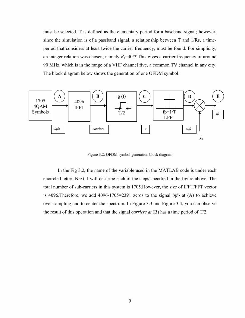
The block diagram below shows the generation of one OFDM symbol:
Figure 3.2: OFDM symbol generation block diagram
In the Fig 3.2, the name of the variable used in the MATLAB code is under each
encircled letter. Next, I will describe each of the steps specified in the figure above. The
total number of sub-carriers in this system is 1705.However, the size of IFFT/FFT vector
is 4096.Therefore, we add 4096-1705=2391 zeros to the signal info at (A) to achieve
over-sampling and to center the spectrum. In Figure 3.3 and Figure 3.4, you can observe
the result of this operation and that the signal carriers at (B) has a time period of T/2.
1705
4QAM Symbols
4096 IFFT
g (t)
T/2
fp=1/T LPF
A B C D E
fc
info carriers u uoft
s(t)

10
0 0.2 0.4 0.6 0.8 1 1.2
x 10-6
-40
-20
0
20
40
60carriers inphase
Time(sec)
Am
plitu
de
0 0.2 0.4 0.6 0.8 1 1.2
x 10-6
-100
-50
0
50
100
150carriers quadrature
Time(sec)
Am
plitu
de
Figure 3.3: Time response of signal carriers
0 0.2 0.4 0.6 0.8 1 1.2 1.4 1.6 1.8 2
x 107
0
0.5
1
1.5carriers FFT
Frequency(Hz)
Am
plitu
de
0 2 4 6 8 10 12 14 16 18
x 106
-90
-80
-70
-60
-50
-40
-30
Frequency(Hz)
Pow
er S
pect
ral D
ensi
ty (d
B/H
z)
carriers Welch PSD estimate
Figure 3.4: Frequency response of signal carriers
The signal carriers are a discrete-time baseband signal. The next step is to produce a
continuous-time signal. In order to achieve this, a transmit filter g (t) is applied to the
complex signal carriers. The impulse response of this filter is shown next:

11
0 1 2 3 4 5 6 7
x 10-8
0
0.1
0.2
0.3
0.4
0.5
0.6
0.7
0.8
0.9
1Pulse g(t)
Time(sec)
Am
plitu
de
Figure 3.5: Impulse response of g (t)
The output of the filter is shown in the following figures, both in time-domain and
frequency-domain.
0 0.2 0.4 0.6 0.8 1 1.2
x 10-6
-40
-20
0
20
40
60u inphase
Time(sec)
Am
plitu
de
0 0.2 0.4 0.6 0.8 1 1.2
x 10-6
-100
-50
0
50
100
150u quadrature
Time(sec)
Am
plitu
de
Figure 3.6: Time response of signal u at (C)

12
0 0.5 1 1.5 2 2.5 3 3.5 4
x 108
0
10
20
30
40
50
Am
plitu
de
Frequency(Hz)
0 0.5 1 1.5 2 2.5 3 3.5
x 108
-120
-100
-80
-60
-40
-20
Frequency (Hz)
Pow
er S
pect
ral D
ensi
ty (d
B/H
z)
Welch PSD Estimate
Figure 3.7: Frequency response of signal u at (C)
The frequency response of Figure 3.7 is periodic, since it is of a discrete-time system.
The bandwidth of the spectrum shown in this figure is given by Rs. The period of the
signal U is 2/T, thus the transition bandwidth for the reconstruction or digital-to-analog
(D/A) filter is (2/T=18.286)-7.61=10.675 MHz. If a 2048-IFFT (N-IFFT) was used, the
transition bandwidth would have been only (1/T=9.143)-7.61=1.533 MHz, which
requires a very sharp roll-off, hence high complexity, in the D/A filter to avoid aliasing.
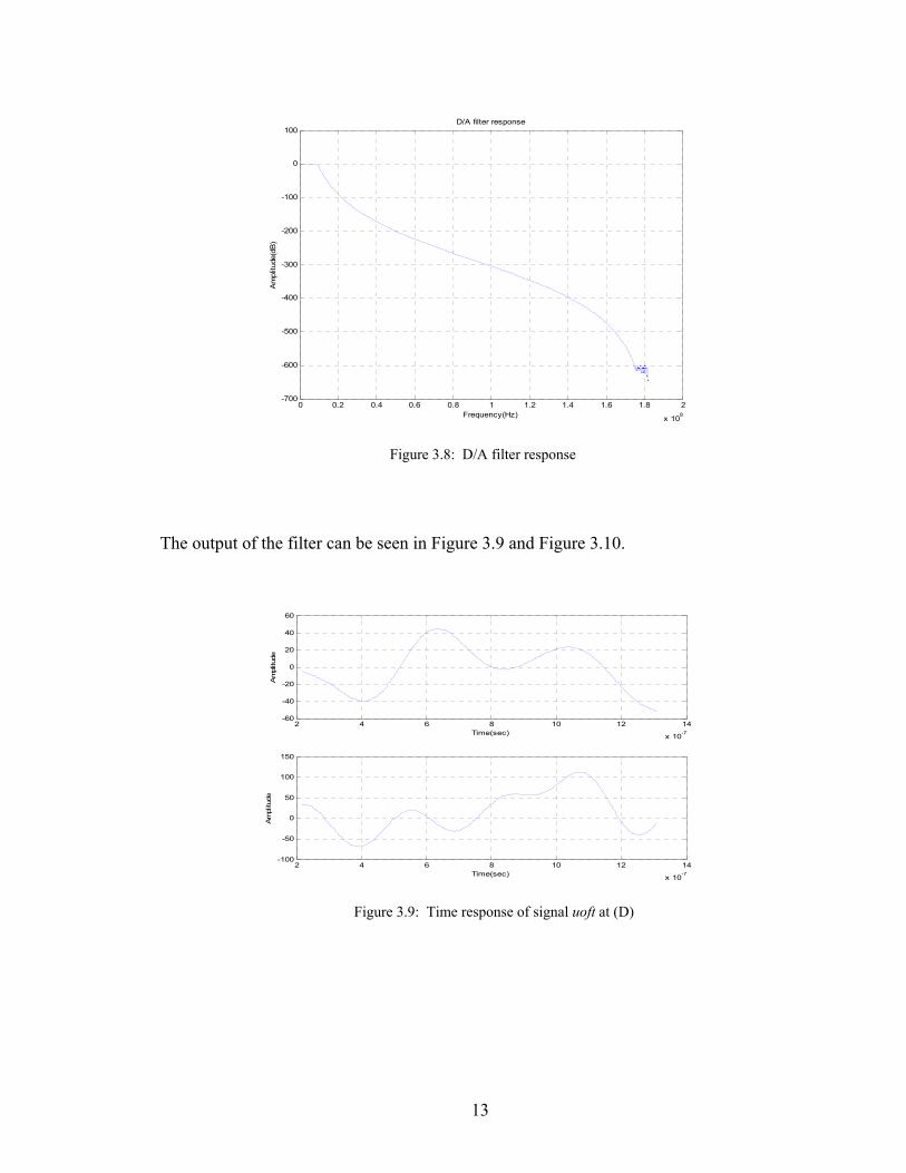
The digital-to-analog (D/A) filter chosen is a Butterworth filter of order 13 and cut-off
frequency close to 1/T.The filter’s response is shown below:
13
0 0.2 0.4 0.6 0.8 1 1.2 1.4 1.6 1.8 2
x 108
-700
-600
-500
-400
-300
-200
-100
0
100D/A filter response
Frequency(Hz)
Am
plitu
de(d
B)
Figure 3.8: D/A filter response
The output of the filter can be seen in Figure 3.9 and Figure 3.10.
2 4 6 8 10 12 14
x 10-7
-60
-40
-20
0
20
40
60
Am
plitu
de
Time(sec)
2 4 6 8 10 12 14
x 10-7
-100
-50
0
50
100
150
Am
plitu
de
Time(sec)
Figure 3.9: Time response of signal uoft at (D)

14
0 0.5 1 1.5 2 2.5 3 3.5 4
x 108
0
10
20
30
40
50uoft FFT
Frequency(Hz)
Am
plitu
de
0 0.5 1 1.5 2 2.5 3 3.5
x 108
-120
-100
-80
-60
-40
-20
Frequency(Hz)
Pow
er S
pect
ral D
ensi
ty (d
B/H
z)uoft Welch PSD estimate
Figure 3.10: Frequency response of signal uoft at (D)
The delay produced by the filtering operation is of approximately 2x10⁻⁷, as it is
obvious when comparing Figure.3.6 and Figure.3.9. Disregarding this, the filtering
performs as expected since we now have only the baseband spectrum. Recall that carriers
1 to 852 are located to the left of 0 Hz and carriers 853 to 1705 are to the right. This
signal is, as mentioned previously, a baseband signal. The next step is to convert it to a
passband signal using quadrature multiplex double-sideband amplitude modulation. In
this type of modulation, an in-phase signal mI (t) and a quadrature signal mQ (t) are
modulated using the formula
( ) ( ) ( ) ( )fctttftts mm QcI ππ 22)( sincos +=
3.4
The in-phase signal corresponds to the real part of the complex modulation symbols,
whereas the quadrature signal corresponds to the imaginary part of the same complex
modulation symbols. For this project, these are 4QAM symbols. Using the formula
above, the signal out of the transmitter s (t) becomes:

15
( ) ( ) ( ) ( )tfttftts cQ
cI uoftuoft ππ 2sin2cos)( +=
3.5
The time and frequency response of the complete OFDM signal s (t) is shown next:
2 4 6 8 10 12 14
x 10-7
-150
-100
-50
0
50
100
150s(t)
Time(sec)
Am
plitu
de
Figure 3.11: Time response of signal s (t) at (E)

16
0 0.5 1 1.5 2 2.5 3 3.5 4
x 108
0
5
10
15
20
25s(t) FFT
Frequency(Hz)A
mpl
itude
0 2 4 6 8 10 12 14 16 18
x 107
-120
-100
-80
-60
-40
-20
Frequency(Hz)
Pow
er S
pect
ral D
ensi
ty (d
B/H
z)
s(t) Welch PSD estimate
Figure 3.12: Frequency response of signal s (t) at (E)
The next step is to transmit the signal through an AWGN channel, receive it and check
the errors. The simulation is based on multiple signal-to-noise-ratio (SNR); meaning that
the signal is received for various SNR values and error check is performed.

17
Chapter 4
OFDM Reception
The design of an OFDM receiver is open since there are only transmission
standards. Most of the research and innovation is done in the receiver. For example, the
frequency sensitivity drawback is mainly a transmission channel prediction problem,
something that is done at the receiver. In this report, I will present only a basic receiver
structure that follows the inverse of the transmission process. The block diagram is
presented in Figure 4.1.
Figure 4.1: An OFDM receiver
OFDM is very sensitive to timing and frequency offsets. The delay produced by the
reconstruction and demodulation filters is about td = 64/Rs for my program. This delay was
taken care of when I did the simulation. As you can see from the block diagram in the
Figure 4.1, the reception process is straightforward: the received OFDM signal is first low-
pass filtered to get the corresponding baseband signal and sampled. The output of the FFT
modulation block is the received constellation. This one passes through a 4QAM slicer,
which assigns the received symbols into the four possible constellation points. The error,
which is a symbol error, is calculated by comparing the original constellation with the one
that is outputted by the 4QAM slicer. As in the case of the transmitter, I indicated the
Fp=2fc
Fs=2/T
4096 FFT
4QAMSlicer
F G H I J
fc
r(t)=s(t)+n
rtilde r_info r_data info_h a_hat

18
names of the variables used in the simulation and the output processes in the reception. The
original constellation is shown in Figure 4.2 whereas the received constellation is shown in
Figure 4.3, Figure 4.4 and Figure 4.5 for corresponding SNR values of 2 dB, 6 dB and 12
dB.
-2 -1.5 -1 -0.5 0 0.5 1 1.5 2-2
-1.5
-1
-0.5
0
0.5
1
1.5
2Original constellation
Figure 4.2: Original 4-QAM constellation

19
-3 -2 -1 0 1 2 3
-2
-1.5
-1
-0.5
0
0.5
1
1.5
2
2.5
infoh Received Constellation
Figure 4.3: Received 4-QAM constellation for SNR=2dB
-2 -1.5 -1 -0.5 0 0.5 1 1.5 2
-1.5
-1
-0.5
0
0.5
1
1.5
infoh Received Constellation
Figure 4.4: Received 4-QAM constellation for SNR=6dB
20
-1.5 -1 -0.5 0 0.5 1 1.5
-1.5
-1
-0.5
0
0.5
1
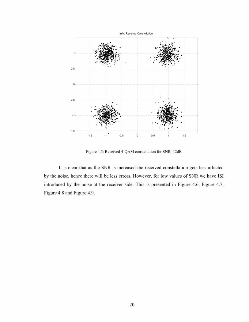
infoh Received Constellation
Figure 4.5: Received 4-QAM constellation for SNR=12dB
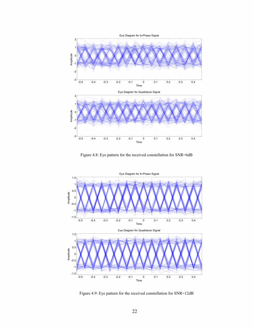
It is clear that as the SNR is increased the received constellation gets less affected
by the noise, hence there will be less errors. However, for low values of SNR we have ISI
introduced by the noise at the receiver side. This is presented in Figure 4.6, Figure 4.7,
Figure 4.8 and Figure 4.9.

21
-0.5 -0.4 -0.3 -0.2 -0.1 0 0.1 0.2 0.3 0.4-1
-0.5
0
0.5
1
Time
Am
plitu
de
Eye Diagram for In-Phase Signal
-0.5 -0.4 -0.3 -0.2 -0.1 0 0.1 0.2 0.3 0.4-1
-0.5
0
0.5
1
Time
Am
plitu
de
Eye Diagram for Quadrature Signal
Figure 4.6: Eye pattern for the received constellation in an ideal channel
-0.5 -0.4 -0.3 -0.2 -0.1 0 0.1 0.2 0.3 0.4-3
-2
-1
0
1
2
3
Time
Am
plitu
de
Eye Diagram for In-Phase Signal
-0.5 -0.4 -0.3 -0.2 -0.1 0 0.1 0.2 0.3 0.4-3
-2
-1
0
1
2
3
Time
Am
plitu
de
Eye Diagram for Quadrature Signal
Figure 4.7: Eye pattern for the received constellation for SNR=2dB
22
-0.5 -0.4 -0.3 -0.2 -0.1 0 0.1 0.2 0.3 0.4-3
-2
-1
0
1
2
Time
Am
plitu
de
Eye Diagram for In-Phase Signal
-0.5 -0.4 -0.3 -0.2 -0.1 0 0.1 0.2 0.3 0.4-3
-2
-1
0
1
2
Time
Am
plitu
de
Eye Diagram for Quadrature Signal
Figure 4.8: Eye pattern for the received constellation for SNR=6dB
-0.5 -0.4 -0.3 -0.2 -0.1 0 0.1 0.2 0.3 0.4-1.5
-1
-0.5
0
0.5
1
1.5
Time
Am
plitu
de
Eye Diagram for In-Phase Signal
-0.5 -0.4 -0.3 -0.2 -0.1 0 0.1 0.2 0.3 0.4-1.5
-1
-0.5
0
0.5
1
1.5
Time
Am
plitu
de
Eye Diagram for Quadrature Signal
Figure 4.9: Eye pattern for the received constellation for SNR=12dB

23
The theoretical probability of symbol error for rectangular QAM constellation is
given in [3] as follows:
( )211 PP MM −−=
4.1
where
( )
⋅−
⋅⋅
−=
NEP M
QM
avM
013112
4.2
Here Eav is the average energy per bit; M = 2k represents the number of levels and
k is the number of bits per symbol. Equations 4.1 and 4.2 are for the case of k even. For k
odd, there is no exact result. However, the symbol-error probability is upper bounded as
( )
⋅−≤
NEP M
kQ av
M01
34
4.3
The result of the simulation is given in Figure 4.10. The theoretical curve was
generated using 4.3, without the scaling factor (i.e. only using the Q-function without the 4
in front), although for my project k was even (i.e. k = 2 for 4QAM). This was suggested in
[3].

24
0 1 2 3 4 5 6 7 810-5
10-4
10-3
10-2
10-1
100
SNR/bit in dB
Sym
bol E
rror R
ate
Simulated error rateTheoretical probability of error
Figure 4.10: Simulated and theoretical symbol error rate

25
Chapter 5
Conclusion
The simulation done in MATLAB worked well. The Additive White Gaussian
Noise (AWGN) corrupted the transmitted signal and this resulted in a different received
4QAM constellation than the original constellation. For small SNR values the calculated
error rate was quite large and ISI was produced due the relative high power of noise. As
SNR was increased the error rate was decreasing, as expected. In fact, for a SNR value
greater than 8 dB, the error was zero. This is a quite different than expected and it is due to
the fact that the program is simulating only 68 OFDM symbols (i.e. one frame), sent one by
one. If the number of transmitted OFDM symbols is increased, than a more accurate error
rate can be obtained, but this necessitates a high processing power PC and time. Letting this
aside, the system’s performance was good since the simulated error rate for small SNR
values was a little bit above the theoretical probability curve. The difference between the
two curves is less than 0.5 dB. As the SNR is increased we observe that the simulated
symbol error rate intersects and then drops below the theoretical error curve. There are
more aspects of OFDM that need to be researched since this simulation was only a basic
one. As an example, there are a lot of improvements that can be brought to the program,
such as the addition of guard interval, coding the original information, simulation over a
multipath channel etc.

26
APPENDIX
MATLAB code used for simulation
clear all;
clc;
close all;
%*********************The 2k DVB-T parameters************************************
Tu=224e-6; %useful OFDM symbol period
T=Tu/2048; %baseband elementary period
G=0; %choice of 1/4, 1/8, 1/15 and 1/32
delta=G*Tu; %guard band duration
Ts=Tu+delta; %total OFDM symbol period
Kmax=1705; %number of subcarriers
Kmin=0;
FS=4096; %IFFT/FFT length
q=10; %carrier period to elementary period ratio
fc=q*1/T; %carrier frequency
Rs=4*fc; %simulation period
t=0:1/Rs:Tu;
tt=0:T/2:Tu;
%*******************************************************************************
repeat=68; % one OFDM frame( 68 OFDM symbols) is sent, symbol by symbol
SNR_dB = 0:2:16 ; %Signal-to-noise ratio in dB
error = zeros(1,length(SNR_dB));
27
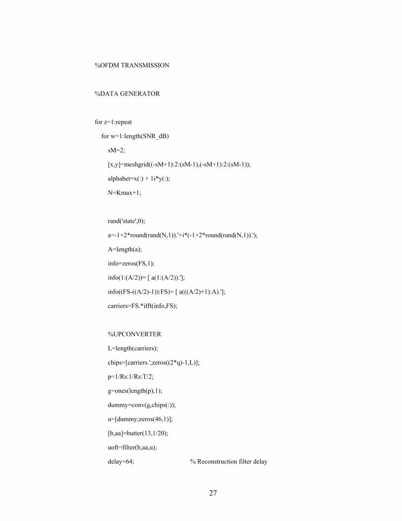
%OFDM TRANSMISSION
%DATA GENERATOR
for z=1:repeat
for w=1:length(SNR_dB)
sM=2;
[x,y]=meshgrid((-sM+1):2:(sM-1),(-sM+1):2:(sM-1));
alphabet=x(:) + 1i*y(:);
N=Kmax+1;
rand('state',0);
a=-1+2*round(rand(N,1)).'+i*(-1+2*round(rand(N,1)).');
A=length(a);
info=zeros(FS,1);
info(1:(A/2))= [ a(1:(A/2)).'];
info((FS-((A/2)-1)):FS)= [ a(((A/2)+1):A).'];
carriers=FS.*ifft(info,FS);
%UPCONVERTER
L=length(carriers);
chips=[carriers.';zeros((2*q)-1,L)];
p=1/Rs:1/Rs:T/2;
g=ones(length(p),1);
dummy=conv(g,chips(:));
u=[dummy;zeros(46,1)];
[b,aa]=butter(13,1/20);
uoft=filter(b,aa,u);
delay=64; % Reconstruction filter delay

28
s_tilde=(uoft(delay+(1:length(t))).').*exp(1i*2*pi*fc*t);
s=real(s_tilde);
%***********************************************************
% Here based on the power of the received signal plus the
% desired SNR we generate and add the AWGN noise to create
% the corrupt signal
noisedst = awgn(s,SNR_dB(w),'measured');
%***********************************************************
%OFDM RECEPTION
%DOWNCONVERTER
r_tilde=exp(-1i*2*pi*fc*t).*noisedst; % (F)
%CARRIER SUPPRESSION
[B,AA]=butter(3,1/2);
r_info=2*filter(B,AA,r_tilde); %Baseband signal continous-time (G)
%SAMPLING
r_data=real(r_info(1:(2*q):length(t)))+1i*imag(r_info(1:(2*q):length(t)));
%Baseband signal discrete-time (H)

29
%FFT
info_2N=(1/FS).*fft(r_data,FS); % (I)
info_h=[info_2N(1:A/2) info_2N((FS-((A/2)-1)):FS)];
%SLICING
for k=1:N,
a_hat(k)=alphabet((info_h(k)-alphabet)==min(info_h(k)-alphabet)); % (J)
end;
figure(1);
plot(info_h((1:A)),'.k');
title('info_h Received Constellation');
axis square;
axis equal;
grid on;
figure(2);
plot(a_hat((1:A)),'or');
title('a_hat 4-QAM');
axis square;
axis equal;
grid on;
axis([-1.5 1.5 -1.5 1.5]);
error(w)= error(w) + length(find(a_hat~=a));
end
end

30
figure(3);
semilogy(SNR_dB,error/(repeat*N),'b<-');
grid on;
ylabel('Symbol Error Rate');
xlabel('SNR/bit in dB')
save result error SNR_dB N repeat
% error,SNR ,N and repeat variables are saved for possible future use
% and to avoid re-runing the simulation
31
REFERENCES
[1] OFDM Simulation using MATLAB. Retrieved May 9, 2003, from http://users.ece.gatech.edu/~mai/tutorial/OFDM/Tutorial_web.pdf
[2] Broadcast papers. Retrieved May 9, 2003, from
http://www.broadcastpapers.com/tvtran/ HarrisDVBTDeliverMobRec01.htm
http://www.broadcastpapers.com/tvtran/ITISMagicsOfDTV10.htm
[3] Proakis, John G. and Salehi, Masoud, Contemporary Communications Systems using MATLAB, CA: Brooks/Cole, 2000.
[4] DVB-T standard. Retrieved May 20, 2003, from
http://www.kjmbc.co.kr/old/beta/ofdm/ofdm.html