regression workshop slides - university of north carolina ... workshop slides.pdf · regression vs....

UNCG Quantitative Methodology Series

Regression Analysis

Scott Richter UNCG-Statistical Consulting Center

Department of Mathematics and Statistics

Regression Analysis Summer 2015

UNCG Quantitative Methodology Series 2

I. Simple linear regression i. Motivating example-runtime 3 ii. Regression details 12 iii. Regression vs. ANOVA 13 iv. Regression “theory” 20 v. Inferences 24 vi. Usefulness of the model 31 vii. Categorical predictors 39

II. Multiple Regression i. Purposes 42 ii. Terminology 43 iii. Quantitative and categorical predictors 50 iv. Polynomial regression 56 v. Several quantitative variables 60

III. Assumptions/Diagnostics i. Assumptions 76

IV. Transformations 80 i. Example 81 ii. Interpretation after log transformation 83

V. Model Building i. Objectives when there are many predictors 85 ii. Multicollinearity 87 iii. Strategy for dealing with many predictors 89 iv. Sequential variable selection 93 v. Cross validation 96



I. Simple Linear Regression

i. Simple Linear Regression--Motivating Example

Foster, Stine and Waterman (1997, pages 191–199)

Variables

o time taken (in minutes) for a production run, Y, and the o number of items produced, X, o 20 randomly selected runs (see Table 2.1 and Figure 2.1).

Want to develop an equation to model the relationship between Y, the run

time, and X, the run size Start with a plot of the data



Scatterplot:

What is the overall pattern? Any striking deviations from that pattern?



Linear model fit

Does this appear to be a valid model?



“it makes sense to base inferences or conclusions only on valid models.” (Simon Sheather, A Modern Approach to Regression with R) But, How can we tell if a model is “valid”?

o Residual plots can be helpful

o Choosing the right plots can be tricky.



Residual plot:

How do we get this plot?

Take the regression fit plot Rotate it until the regression line is horizontal and explode



Now…what are we looking for in the residual plot?

o Random scatter around 0-line suggests valid model

o May or may not be a useful model! (“essentially, all models are wrong, but some are useful.” --George E. P. Box)

If we believe the model to be valid, we may proceed to interpret:



Parameter estimates from software:

Variable DF ParameterEstimate

StandardError

t Value Pr > |t| 95% Confidence Limits

Intercept 1 149.74770 8.32815 17.98 <.0001 132.25091 167.24450RunSize 1 0.25924 0.03714 6.98 <.0001 0.18121 0.33728

Interpretation: For each additional item produced, the average runtime is estimated to

increase by 0.26 minutes (about 15s).

Estimate is statistically different from 0 (p < 0.0001; at least 0.18 with 95% confidence)

Can safely be applied to runs of about between 50 to 350 items



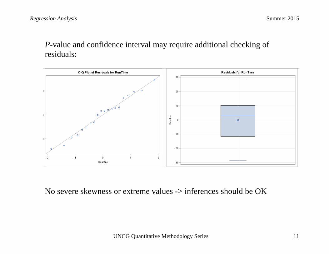
P-value and confidence interval may require additional checking of residuals:

No severe skewness or extreme values -> inferences should be OK



ii. Simple Linear Regression--Some details Data consist of a set of bivariate pairs (Yi, Xi)

The data arise either as

o a random sample of pairs from a population, o random samples of Y’s selected independently from several fixed

values Xi , or o an intact population

The X-variable

o is usually thought of as a potential predictor of the Y-variable o values can sometimes be chosen by the researcher

Simple linear regression is used to model the relationship between Y

and X so that given a specific value of X o we can predict the value of Y or o estimate the mean of the distribution of Y.



iii. Simple Linear Regression--Regression vs. ANOVA Another example: Concrete. (From Vardeman (1994), Statistics for Engineering Problem Solving) A study was performed to investigate the relationship between the strength (psi) of concrete and water/cement ratio. Three settings of water to cement were chosen (0.45, 0.50, 0.55). For each setting 3 batches of concrete were made. Each batch was measured for strength 14 days later. All other variables were kept constant (mix time, quantity of batch, same mixer used (which was cleaned after every use), etc.). The data: Water/cement 0.45 0.45 0.45 0.50 0.50 0.50 0.55 0.55 0.55 Strength 2824 2753 2803 2743 2789 2709 2662 2737 2703

o Essentially 3 “groups”: 45%, 50%, 55%

o Can use one-way ANOVA to compare means



Boxplots:

Suggests evidence that

o means are different o means decrease as ratio increases



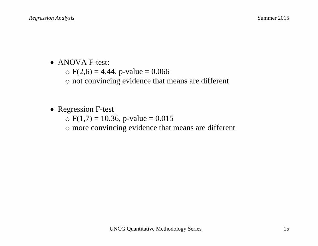
ANOVA F-test:

o F(2,6) = 4.44, p-value = 0.066 o not convincing evidence that means are different

Regression F-test

o F(1,7) = 10.36, p-value = 0.015 o more convincing evidence that means are different



Why different results?

More specific regression alternative: means follow a linear relation

Only one parameter estimate needed (instead of 2)

Regression ANOVA Source DF SS MS F value Pr > F

Model 1 12881 12881 10.36 0.015

Error 7 8705.33 1243.62

Corrected Total

8 21586

Source DF SS MS F Value Pr > F

Model 2 12881 6440.33 4.44 0.066

Error 6 8705.33 1450.89

Corrected Total

8 21586

Will regression always be more powerful if predictor is numeric?



Suppose the pattern was different:

Water/cement 0.45 0.45 0.45 0.50 0.50 0.50 0.55 0.55 0.55 Strength 2743 2789 2709 2824 2753 2803 2662 2737 2703



ANOVA F-test: o F(2,6) = 4.44, p-value = 0.066 (no change because the sample

means are the same) Regression F-test

o F(1,7) = 1.23, p-value = 0.305 o now, less convincing evidence that means are different o linear model is not valid for these data



Residual plot shows a non-random pattern (possibly quadratic?):



iv. Simple Linear Regression--A little bit of theory and notation. Simple linear regression model:

0 1|Y X X

|Y X represents the population mean of Y for a given setting of X

0 is the intercept of the linear function

1 is the slope of the linear function (All of these are unknown parameters.)



Method of Least Squares 1. The fitted value for observation i is its estimated mean: 0 1

ˆ ˆifit X

2. The residual for observation i is: i i ires Y fit 3. The method of least squares finds 0̂ and 1̂ that minimize the sum of squared residuals.



Estimates for Runsize/Runtime example:

o 0ˆ 149.75

o 1̂ 0.26

o 149.75 0.26*ifit Runtime



v. Simple Linear Regression--Inferences

Three types:

1) Inferences about the regression parameters (most common)

Variable DF Parameter

EstimateStandard

Errort Value Pr > |t| 95% Confidence Limits


1. Each row gives a test for evidence that the parameter equals 0:




EstimateStandard



a. 1st row: 0 0: 0H Average Runtime=0 when Runsize=0

i. Test statistic: 149.75 17.988.33

t

ii. p-value: <0.0001

iii. strong evidence that 0 0

iv. often not practically meaningful




EstimateStandard



b. 2nd row: 0 1: 0H best fitting line has slope=0

i. Test statistic: 0.26 6.980.04

t

ii. p-value: <0.0001

iii. strong evidence that 1 0

1. “Evidence of linear relation” 2. Not necessarily evidence of valid model! (example later)



2) Estimation of the mean of Y for a given setting of X: Suppose Runsize =

200 Estimated mean Runtime is 201.6

95% confidence interval: (194.0, 209.2)

“With 95% confidence, the mean Runtime for all runs of size 200 is

between 194.0 and 209.2 minutes.



3) Prediction of a single, future value of Y given X: Suppose Runsize = 200

Predicted Runtime is 201.6

95% confidence interval: (166.6, 236.6)

“With 95% confidence, any single Runtime for run of size 200 will be

between 166.6 and 236.6 minutes.



Features of confidence/prediction limits Most narrow at mean of X--wider as you move away from mean Intervals for means can be made as small as we want by increasing

sample size--Prediction intervals cannot



Cautions Estimates/Predictions should only be made for valid models

Estimates/Predictions should only be made within the range of

observed X values

Extrapolation should be avoided--unknown whether the model extends beyond the range of observed values



vi. Simple Linear Regression--Assessing usefulness of the model How much is the residual error reduced by using the regression?

2R : Coefficient of determination—measures proportional reduction in residual error.



Idea: Consider Runtime vs. Runsize example Ignore X and compute the mean and variance of Y

mean = 4041 202.0520

sumYn

variance =

2

1( )

17622.95 927.521 1 19

n

ii

Y Ycorrected SS

n n

Include X and compute the fitted values and pooled variance of Y

V(Y) = 2

1 (Residual) 47 264.1454.582 2 18

n

i ii

Y fitSS

n n



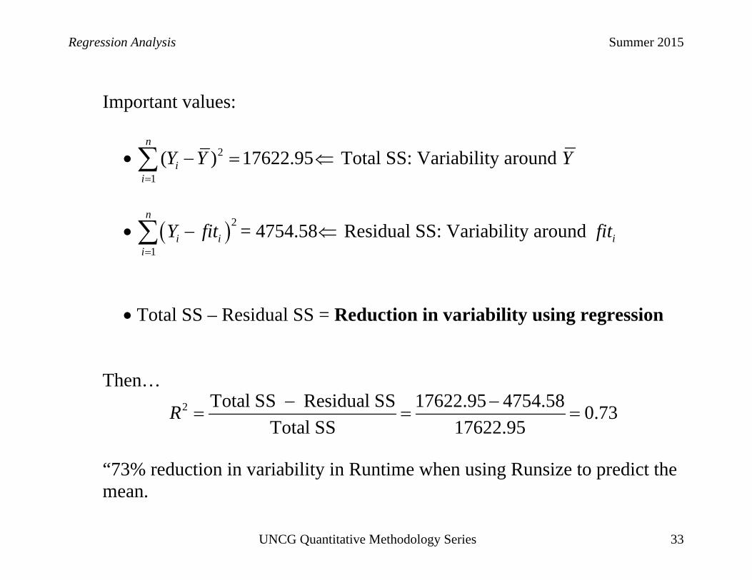
Important values:

2

1

( ) 17622.95n

ii

Y Y

Total SS: Variability around Y

2

1

n

i ii

Y fit

= 4754.58 Residual SS: Variability around ifit

Total SS – Residual SS = Reduction in variability using regression Then…

2 Total SS Residual SS 17622.95 4754.58 0.73Total SS 17622.95

R

“73% reduction in variability in Runtime when using Runsize to predict the mean.



SAS Output:

Source DF Sum ofSquares

Mean Square

F Value Pr > F

Model 1 12868 12868 48.72 <.0001Error 18 4754.58 264.14 Corrected Total 19 17623

Root MSE 16.25248 R-Square 0.7302



A picture is worth…(http://en.wikipedia.org/wiki/Coefficient_of_determination)

The areas of the blue squares represent the squared residuals with respect to the linear regression. The areas of the red squares represent the squared residuals with respect to the average value.



Interpreting 2R

If X is no help at all in predicting Y (slope = 0) then 2 0R .

If X can be used to predict Y exactly 2 1R .

2R is useful as a unitless summary of the strength of linear association

2R is NOT useful for assessing model adequacy or significance



Example: Chromatography Linear model fit to relate the reading of a gas chromatograph to the actual amount of substance present to detect in a sample. 2 0.9995R !



Residual plot

Indicates the need for a nonlinear model Predicted values from the linear model will be “close” but systematically

biased



vii. Simple Linear Regression--Regression with categorical predictors Example-Menu pricing data. You have been asked to determine the pricing of a restaurant’s dinner menu so that it is competitively positioned with other high-end Italian restaurants in the area. In particular, you are to produce a regression model to predict the price of dinner. Data from surveys of customers of 168 Italian restaurants in the area are available. The data are in the form of the average of customer views on:

Price = the price (in $) of dinner (including one drink & a tip) Food = customer rating of the food (out of 30) Décor = customer rating of the decor (out of 30) Service = customer rating of the service (out of 30) East = 1 (0) if the restaurant is east (west) of Fifth Avenue

The restaurant owners also believe that views of customers (especially regarding Service) will depend on whether the restaurant is east or west of 5th Ave.



Compare prices: east versus west 1. t-test

East N Mean 0 62 40.4355 1 106 44.0189

West(0) mean – East(1) mean: 40.44 – 44.02 = 3.58

Test statistic: t (166 df) = -2.45, p-value = 0.015.



2. Regression

Create an indicator/dummy variable

1, if East of 5th0, if West of 5th

East

Fit regression model with East as predictor

Output:

Variable DF ParameterEstimate

Standard Error

t Value Pr > |t|

Intercept 1 40.43548 1.16294 34.77 <.0001East 1 3.58338 1.46406 2.45 0.0154

o 3.58 = East(1) mean – West(1) mean o t (166 df) = 2.45, p-value = 0.015



II. Multiple Regression

i. Some purposes of multiple regression analysis: 1. Examine a relationship between Y and X after accounting for other variables 2. Prediction of future Y’s at some values of X1, X2, … 3. Test a theory 4. Find “important” X’s for predicting Y (use with caution!) 5. Get mean of Y adjusted for X1, X2, … 6. Find a setting of X1, X2, … to maximize the mean of Y (response surface methodology)



ii. Multiple Linear Regression--Terminology

1. The regression of Y on X1 and X2: (Y|X1,X2) = “the mean of Y as a function of X1 and X2” 2. Regression model: a formula to approximate (Y|X1,X2)

Example: (Y|X1,X2) = 0 + 1X1 + 2X2 3. Linear regression model: a regression model linear in s 4. Regression analysis: tools for answering questions via regression models



Things to remember:

1. Interpretation of the effect of explanatory variable assumes the others can be held constant. 2. Interpretation depends on which other predictors are included in the model (and which are not). 3. Interpretation of causation requires random assignment.



iii. Multiple Linear Regression--Quantitative and categorical predictors Travel example. A travel agency wants to better understand two important customer segments. The first segment (A), are customers who purchased an adventure tour in the last twelve months. The second segment (C), are customers who purchased a cultural tour in the last twelve months. Data are available on 466 customers from segment A and 459 from segment C. (there are no customers who are in both segments). Interest centers on identifying any differences between the two segments in terms of the amount of money spent in the last twelve months. In addition, data are also available on the age of each customer, since age is thought to have an effect on the amount spent.



Consider first simple (one predictor) models:

1. Age as predictor

Model: 0 1|Amount Age Age Output:

Source DF SS MS F Value Pr > FModel 1 152397 152397 2.70 0.1009Error 923 52158945 56510Corrected Total 924 52311342Root MSE 237.71881 R-Square 0.0029

Parameter Estimates

Variable DF Estimate SE t Value Pr > |t|Intercept 1 957.91033 31.30557 30.60 <.0001Age 1 -1.11405 0.67839 -1.64 0.1009



2. Segment as predictor

Model: 0 1|Amount C C

1, if Cultural tour0, if Adventure tour

C

Output: Source DF SS MS F Value Pr > FModel 1 44257 44257 0.78 0.3769Error 923 52267084 56627 Corrected Total 924 52311342 Root MSE 237.96511 R-Square 0.0008

Parameter Estimates

Variable DF Estimate SE t Value Pr > |t|Intercept 1 914.99356 11.02352 83.00 <.0001C 1 -13.83452 15.64894 -0.88 0.3769



3. Both Age and Segment as predictors Model: 0 1 2| ,Amount C Age C Age Output:

Source DF SS MS F Value Pr > FModel 2 191001 95500 1.69 0.1852Error 922 52120341 56530 Corrected Total 924 52311342 Root MSE 237.75966 R-Square 0.0037

Parameter Estimates

Variable DF Estimate SE t Value Pr > |t|Intercept 1 963.42541 32.01430 30.09 <.0001Age 1 -1.09389 0.67894 -1.61 0.1075C 1 -12.92908 15.64552 -0.83 0.4088



How to interpret the estimates in this model?

Hint: Plot of predicted values:

Age: -1.09 is the slope of the regression of Amount by Age (same for

both segments)

C: -12.93 is the mean difference between C and A groups (“gap”)



We should have done this at the start, but…here is the scatterplot:

We now see why the coefficients of the simple regressions were not significant!



Residual plot from 0 1 2| ,Amount C Age C Age :

Clearly a pattern which suggests an invalid model!



The scatterplot suggests A and C groups have different slopes. Fit the separate slopes model: Model: 0 1 2 3| , *Amount C Age C Age C Age Output:

Source DF SS MS F Value Pr > FModel 3 50221965 16740655 7379.30 <.0001Error 921 2089377 2268.59616Corrected Total 924 52311342Root MSE 47.62978 R-Square 0.9601

Parameter Estimates

Variable DF Estimate SE t Value Pr > |t|Intercept 1 1814.54449 8.60106 210.97 <.0001Age 1 -20.31750 0.18777 -108.21 <.0001C 1 -1821.23368 12.57363 -144.85 <.0001int 1 40.44611 0.27236 148.50 <.0001



Predicted values:



We need to be careful, however, since the interpretation of the estimates is now different from previous models Model: 0 1 2 3| , *Amount C Age C Age C Age If C = 1:

0 1 2 3

0 1 2 3

| 1,Amount C Age Age Age

Age

If C = 0: 0 2| 0,Amount C Age Age

1 = mean difference when Age = 0 only. 2 = slope only for C = 0 (Adventure group) 3 = difference in slopes (C versus A)

*Note that none of these gives “effect of Age” or “effect of segment”



Residual plot of separate slopes model:

No indication model is not valid.



iv. Multiple Linear Regression--Polynomial regression Example: Modeling salary from years of experience

Y = salary; X = years experience 1) Scatterplot--Suggests nonlinear relation



2) Fit linear model ( 0 1|Y X X ) to data.

Source DF SS MS F Value Pr > F

Model 1 9962.93 9962.93 293.33 <.0001

Error 141 4789.05 33.96Corrected Total 142 14752Root MSE 5.82794 R-Square 0.6754 Variable DF Estimate SE t Value Pr > |t|Intercept 1 48.51 1.09 44.58 <.0001exper 1 0.88 0.05 17.13 <.0001

Evidence of nonzero slope, but wait: is this a valid model?



Fitted values Residuals

Note that even though the fitted line has nonzero slope, the residual plot reveals the linear model is not valid. Plot suggests quadratic function may be more appropriate



Add quadratic term: 2

0 1 2|Y X X X

Fitted values Residuals

Looks much better!



Parameter estimates--Quadratic model

Source DF SS MS F Value Pr > FModel 2 13641 6820.39 859.31 <.0001Error 140 1111.18 7.94Corrected Total 142 14752Root MSE 2.82 R-Square 0.92 Variable DF Estimate SE

t Value Pr > |t|

Intercept 1 34.72 0.83 41.90 <.0001exper 1 2.87 0.10 30.01 <.0001expsq 1 -0.05 0.002 -21.53 <.0001

Statistically significant terms suggest both linear and quadratic terms needed.



v. Multiple Linear Regression--Several quantitative variables Pulse data. Students in an introductory statistics class participated in the following experiment. The students took their own pulse rate, then were asked to flip a coin. If the coin came up heads, they were to run in place for one minute, otherwise they sat for one minute. Then everyone took their pulse again. Other physiological and lifestyle data were also collected. Variable Description Height Height (cm) Weight Weight (kg) Age Age (years) Gender Sex Smokes Regular smoker? (1 = yes, 2 = no) Alcohol Regular drinker? (1 = yes, 2 = no) Exercise Frequency of exercise (1 = high, 2 = moderate, 3 = low) Ran Whether the student ran or sat between the first and second pulse

measurements (1 = ran, 2 = sat) Pulse1 First pulse measurement (rate per minute) Pulse2 Second pulse measurement (rate per minute) Year Year of class (93 - 98)



Want to predict Pulse1 using Age, Height, Weight and Gender Determine if separate models for Gender are needed Common practice that should be avoided: test for gender mean difference

Gender N Mean Std Dev Std Err0 50 77.5000 12.6285 1.78591 59 74.1525 13.7588 1.7912 Method Variances DF t Value Pr > |t|Pooled Equal 107 1.31 0.1917Satterthwaite Unequal 106.3 1.32 0.1885

No evidence of gender mean difference. However, this does not address the research question



Better approach: Fit model with desired predictors Check for interaction

Model with desired predictors (reduced model):

0 1 2 3 41|Pulse X Height Weight Age Gender Add interaction terms (full model):

0 1 2 3 4

5 6 7

1|* * *

Pulse X Height Weight Age GenderGen Height Gen Weight Gen Age

Fit both models and assess change in fit



Full model: Source DF SS MS F Value Pr > FModel 7 3242.86133 463.26590 2.95 0.0074Error 101 15855 156.97558Corrected Total 108 19097Root MSE 12.52899 R-Square 0.1698Dependent Mean 75.68807 Adj R-Sq 0.1123

Parameter Estimates

Variable DF Estimate SE t Value Pr > |t|Intercept 1 177.89940 30.76414 5.78 <.0001Height 1 -0.37491 0.19563 -1.92 0.0581Weight 1 -0.28927 0.26109 -1.11 0.2705Age 1 -1.12100 0.65155 -1.72 0.0884Gender 1 -81.49376 36.33879 -2.24 0.0271gen_height 1 0.25098 0.22389 1.12 0.2649gen_weight 1 0.37058 0.28970 1.28 0.2038gen_age 1 0.82092 0.74376 1.10 0.2723



Reduced model:

Source DF SS MS F Value Pr > FModel 4 1858.64050 464.66013 2.80 0.0295Error 104 17239 165.75725Corrected Total 108 19097Root MSE 12.87467 R-Square 0.0973Dependent Mean 75.68807 Adj R-Sq 0.0626

Parameter Estimates

Variable DF Estimate SE t Value Pr > |t|Intercept 1 124.10482 15.58478 7.96 <.0001Height 1 -0.21719 0.09495 -2.29 0.0242Weight 1 -0.02958 0.11517 -0.26 0.7978Age 1 -0.46136 0.31930 -1.44 0.1515Gender 1 0.55307 3.11838 0.18 0.8596



Test change in model fit ( 0 :H all three interaction coefficients = 0):

(Reduced) (Full) 17239 15855 1384 SSSSError SSError Extra

(Reduced) (Full) 104 101 3dfError dfError dfExtra

then 1384 461.43

SSExtraMSExtradfExtra

.

Finally, 461.4 2.94(Full) 156.98

MSExtraFMS

, with 3,101 df.

p-value = 0.037 evidence interaction terms are needed



Software will generally do this

From SAS:

Test gen_int Results for Dependent Variable Pulse1Source DF Mean

SquareF Value Pr > F

Numerator 3 461.40694 2.94 0.0368Denominator 101 156.97558



Interpreting individual coefficients Back to Menu Pricing: You are to produce a regression model to predict the price of dinner, based on data from surveys of customers of 168 Italian restaurants in the area. Variables:

Price = the price (in $) of dinner (including one drink & a tip) Food = customer rating of the food (out of 30) Décor = customer rating of the decor (out of 30) Service = customer rating of the service (out of 30) East = 1 (0) if the restaurant is east (west) of Fifth Avenue



Scatterplot matrix Assess possible functional form of association with price Identify potential outliers Assess degree of multicollinearity



Fit linear model: 0 1 2 3 4Price | X Food Decor Service East

Source DF SS MS F Value Pr > FModel 4 9054.99614 2263.74904 68.76 <.0001Error 163 5366.52172 32.92345Corrected Total 167 14422Root MSE 5.73790 R-Square 0.6279 Adj R-Sq 0.6187

Variable DF Estimate SE t Value Pr > |t|Intercept 1 -24.02380 4.70836 -5.10 <.0001Food 1 1.53812 0.36895 4.17 <.0001Decor 1 1.91009 0.21700 8.80 <.0001Service 1 -0.00273 0.39623 -0.01 0.9945East 1 2.06805 0.94674 2.18 0.0304

Should Service be removed?



Residual plot



Results of model after removing Service:

Source DF SS MS F Value Pr > FModel 3 9054.99458 3018.33153 92.24 <.0001Error 164 5366.52328 32.72270Corrected Total 167 14422Root MSE 5.72038 R-Square 0.6279Dependent Mean 42.69643 Adj R-Sq 0.6211

Parameter Estimates

Variable DF Estimate StError t Value Pr > |t|Intercept 1 -24.02688 4.67274 -5.14 <.0001Food 1 1.53635 0.26318 5.84 <.0001Decor 1 1.90937 0.19002 10.05 <.0001East 1 2.06701 0.93181 2.22 0.0279

Virtually no change in parameter estimates. Standard errors all decrease (slightly). Appears to be a valid model.



Interpretation of individual coefficients Effect of Food on Price: “Each one point increase in average rating of Food

is associated with a $1.54 increase in the Price of a meal, assuming Décor rating and location (East/West) do not change.”

Difficulty 1: Is the assumption that Food rating can change while Décor and

location do not reasonable or plausible? Maybe not.

Pearson Correlation Coefficients, N = 168 Prob > |r| under H0: Rho=0

Food Decor EastFood 1.00000 0.50392

<.0001

0.180370.0193

1.00000

0.035750.6455

1.00000



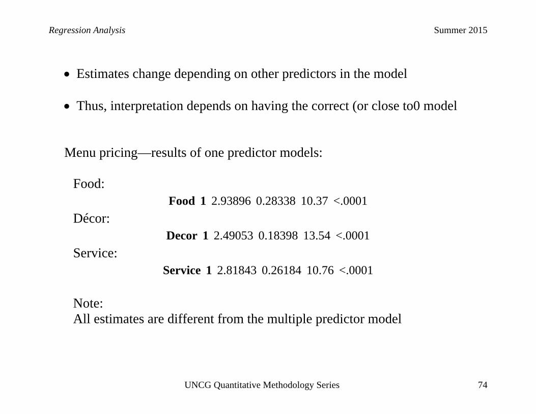
Estimates change depending on other predictors in the model

Thus, interpretation depends on having the correct (or close to0 model

Menu pricing—results of one predictor models: Food:

Food 1 2.93896 0.28338 10.37 <.0001Décor:

Decor 1 2.49053 0.18398 13.54 <.0001Service:

Service 1 2.81843 0.26184 10.76 <.0001

Note: All estimates are different from the multiple predictor model



Interpreting individual coefficients again: Pulse data Parameter Estimates

Variable DF Estimate SE t Value Pr > |t|Intercept 1 177.89940 30.76414 5.78 <.0001Height 1 -0.37491 0.19563 -1.92 0.0581Weight 1 -0.28927 0.26109 -1.11 0.2705Age 1 -1.12100 0.65155 -1.72 0.0884Gender 1 -81.49376 36.33879 -2.24 0.0271gen_height 1 0.25098 0.22389 1.12 0.2649gen_weight 1 0.37058 0.28970 1.28 0.2038gen_age 1 0.82092 0.74376 1.10 0.2723

What is the effect of Weight on pulse1? Weight coefficient—represents estimate for Gender=0) group only

o Weight(Gender=0) = -0.29 o Weight(Gender=1) = -0.29 + 0.37 = 0.08. o Decrease for Gender = 0, increase for Gender = 1!

Again, these both assume Height and Age do not change…



III. Assumptions/Diagnostics i. Assumptions

1. Linearity—Very important a. Curvature b. Outliers c. Can cause biased estimates, inaccurate inferences d. Severity depends on severity of violation e. Remedies

i. transformations ii. nonlinear models (especially polynomials)

2. Equal variance—Very important

a. Tests and CIs can be misleading b. Remedies

i. transformation ii. weighted regression



3. Normality

a. Important for prediction intervals b. Otherwise, not important unless

i. extreme outliers are present, and ii. samples sizes are small

c. Remedies i. transformation

ii. outlier strategy

4. Independence a. Important, as before—Usually serial correlation or clustering b. Remedies

i. Adding more explanatory variables ii. Modeling serial correlation



Assessing Model Assumptions—Graphical Methods

Scatterplots

1. Response variable vs. explanatory variable

2. (Studentized) Residuals vs. fitted/explanatory variable a. Linearity b. Equal variance c. Outliers

3. (Studentized) Residuals vs. time

a. Serial correlation b. Trend over time

Normality plots

1. Normal plots 2. Boxplots/Histograms



Summary of robustness and resistance of least squares

Assumptions

The linearity assumption is very important (probably most)

The “constant variance” assumption is important

Normality o is not too important for confidence intervals and p-values—larger

sample size helps o is important for prediction intervals—larger sample size does not help

much

Long-tailed distributions and/or outliers can heavily influence the results



IV. Transformations

Can sometimes be used to induce linearity

Many options: o polynomial (square, cube, etc.) o roots (square, cube etc.) o log o inverse

o logit 1

pp

OK if p-value is all that is needed

Log is an exception



i. Transformations--Example: Breakdown times for insulating fluid under different voltages. Fit 0 1|Time Voltage Voltage Plots reveal model is invalid



Try log transformation of Time: 0 1ln( ) |Time Voltage Voltage

Variable DF Estimate SE t Value Pr > |t|Intercept 1 18.95546 1.91002 9.92 <.0001VOLTAGE 1 -0.50736 0.05740 -8.84 <.0001



ii. Transformations--Interpretation after log transformation

1. If response is logged:

o 0 1{ | } log Y X X is the same as: Median{Y|X} = 0 1Xe (if the distribution of log(Y) given X is symmetric)

o “As X increases by 1, the median of Y changes by the multiplicative

factor of 1e .”

o Voltage example: Unit increase in voltage associated with a in Time to 0.5 * 0.61*e Time Time , i.e., average Time decreases by 39%.

2. If predictor is logged:

o 0 1{ | log( )} log( )Y X X , 1{ | log( )} { | log( )} log( )Y cX Y X c



o “Associated with each c-fold increase of X is a 1 log( )c change in the mean of Y.”

o Suppose 2c . Then: “Associated with each two-fold increase (i.e.

doubling) of X is a 1 log(2) change in the mean of Y.” 3. If both Y and X are logged:

o 0 1{log( ) | log( )} log( )Y X X

o If X is multiplied by c, the median of Y is multiplied by 1c



V. Model Building

i. Objectives when there are many predictors 1. Assessment of one predictor, after accounting for many others Example: Do males receive higher salaries than females, after accounting

for legitimate determinants of salary?

o Strategy:

first find a good set of predictors to explain salary

then see if the sex indicator is significant when added in



2. Fishing for association; i.e. what are the “important” predictors? Regression is not well suited to answer this question

The trouble with this: usually can find several subsets of X’s that

explain Y, but that doesn’t imply importance or causation

Best attitude: use this for hypothesis generation, not testing 3. Prediction (this is a straightforward objective) Find a useful set of predictors;

No interpretation of predictors required



ii. Model Building--Multicollinearity: the situation in which 2jR is large for one

or more j’s (usually characterized by highly correlated predictors)



The standard error of prediction will also tend to be larger if there are

unnecessary or redundant X’s in the model

There isn’t a real need to decide whether multicollinearity is or isn’t present, as long as one tries to find a subset of predictors that adequately explains ( )Y , without redundancies



iii. Model Building--Strategy for dealing with many predictors 1. Identify objectives; identify relevant set of X’s 2. Exploration: matrix of scatterplots; correlation matrix; residual plots after fitting tentative models 3. Resolve transformation and influence before variable selection 4. Computer-assisted variable selection

a. Best: Compare all possible subset models using either Cp, AIC, or BIC

b. If (a) is not feasible: Use sequential variable selection, like stepwise regression (see warnings below)*

doesn’t consider possible subset models, but may be more convenient with some statistical programs



Heuristics for selecting from among all subsets

1. 2 ( ) ( )( )

SS Total SS ErrorRSS Total

a. Larger is better b. However, will always go up when additional X’s are added c. Not very useful for model selection

2. Adjusted R2

2 ( ) / ( 1) ( ) / ( ) ( ) ( )( ) / ( 1) ( )

SS Total n SS Error n p MS Total MS ErrorRSS Total n MS Total

a. Larger is better b. Only goes up if MSE goes down c. “Adjusts” for the number of explanatory variables d. Better than R2, but others are usually better



3. Mallow’s Cp

a. Idea: i. Too few explanatory variables: biased estimates

ii. Too many explanatory variables: increased variance iii. Good model will have both small bias and small variance

b. Smaller is better c. Assumes the model with all candidate explanatory variables is

unbiased 4. Aikaike’s Information Criterion (AIC) and Schwarz’s Bayesian

Information Criterion (BIC) a. Both include a measure of variance (lack-of-fit) plus a penalty for

more explanatory variables b. Smaller is better



No way to truly say that one of these criteria is better than the others

Strategy: Fit all possible models; report the best 10 or so according to the

selected criteria (hopefully all more or less agree) Use theory and common sense to choose “best” model

Regardless of what the heuristics suggest, add and drop factor indicator

variables as a group



iv. *Model Building--Sequential variable selection “Never let a computer select predictors mechanically. The computer does not know your research questions nor the literature upon which they rest. It cannot distinguish predictors of direct substantive interest from those whose effects you want to control.” Singer & Willet (2003)

Here are some of the problems with stepwise variable selection. Yields R-squared values that are badly biased high p-values and CI’s for variables in the selected model cannot be taken

seriously—because of serious data snooping (applies to Objective 2 only) Gives biased regression coefficients that need shrinkage (the coefficients for

remaining variables are too large; see Tibshirani, 1996). It has severe problems in the presence of collinearity. It is based on methods intended to be used to test pre-specified hypotheses. Increasing the sample size doesn't help very much The product is a single model, which is deceptive. Think not: “here is the

best model.” Think instead: “here is one, possibly useful model.” It allows us to not think about the problem.



How automatic selection methods work

1. Forward selection a. Start with no X’s “in” the model b. Find the “most significant” additional X (with an F-test) c. If its p-value is less than some cutoff (like .05) add it to the model (and re-fit the model with the new set of X’s) d. Repeat (b) and (c) until no further X’s can be added e. Weakness: once a variable is entered, it cannot be later removed

2. Backward elimination a. Start with all X’s “in” the model b. Find the “least significant” of the X’s currently in the model c. If it’s p-value is greater than some cutoff (like .05) drop it from the model (and re-fit with the remaining x’s) d. Repeat until no further X’s can be dropped e. Weakness: once a variable is dropped, it cannot be later re-entered



3. (Forward or Backward) Stepwise regression a. Start with no (or all) X’s “in” b. Do one step of forward (or backward) selection c. Do one step of backward (or forward) elimination d. Repeat (b) and (c) until no further X’s can be added or dropped e. A variable can re-enter the model after being dropped at an earlier step.



v. Model Building--Cross Validation If tests, CIs, or prediction intervals are needed after variable selection

and if n is large, try cross validation Randomly divide the data into 75% for model construction and 25% for

inference Perform variable selection with the 75%

Refit the same model (don’t drop or add anything) on the remaining

25% and proceed with inference using that fit

regression workshop slides - university of north carolina ... workshop slides.pdf · regression vs....

Documents