Regression and correlation analysis (RaKA)

1

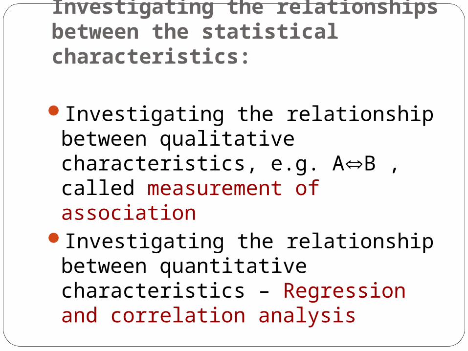
Investigating the relationships between the statistical characteristics:

2

Investigating the relationship between qualitative characteristics, e.g. AB , called measurement of association

Investigating the relationship between quantitative characteristics – Regression and correlation analysis

3

Regression and correlation analysis:

4

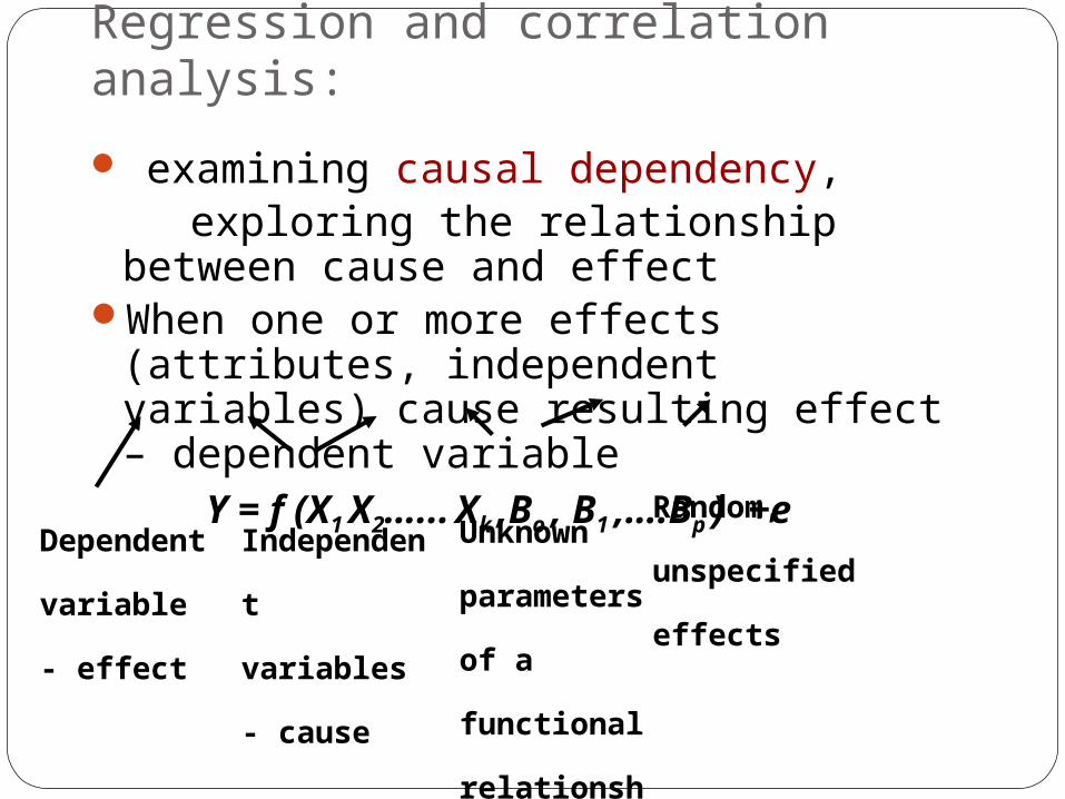
examining causal dependency, exploring the relationship between

cause and effectWhen one or more effects (attributes,

independent variables) cause resulting effect – dependent variable

Y = f (X1 X2…... Xk ,Bo , B1 ,….Bp ) +e

Dependent

variable

- effect

Independent

variables

- cause

Unknown

parameters of

a functional relationship

Random,

unspecified effects

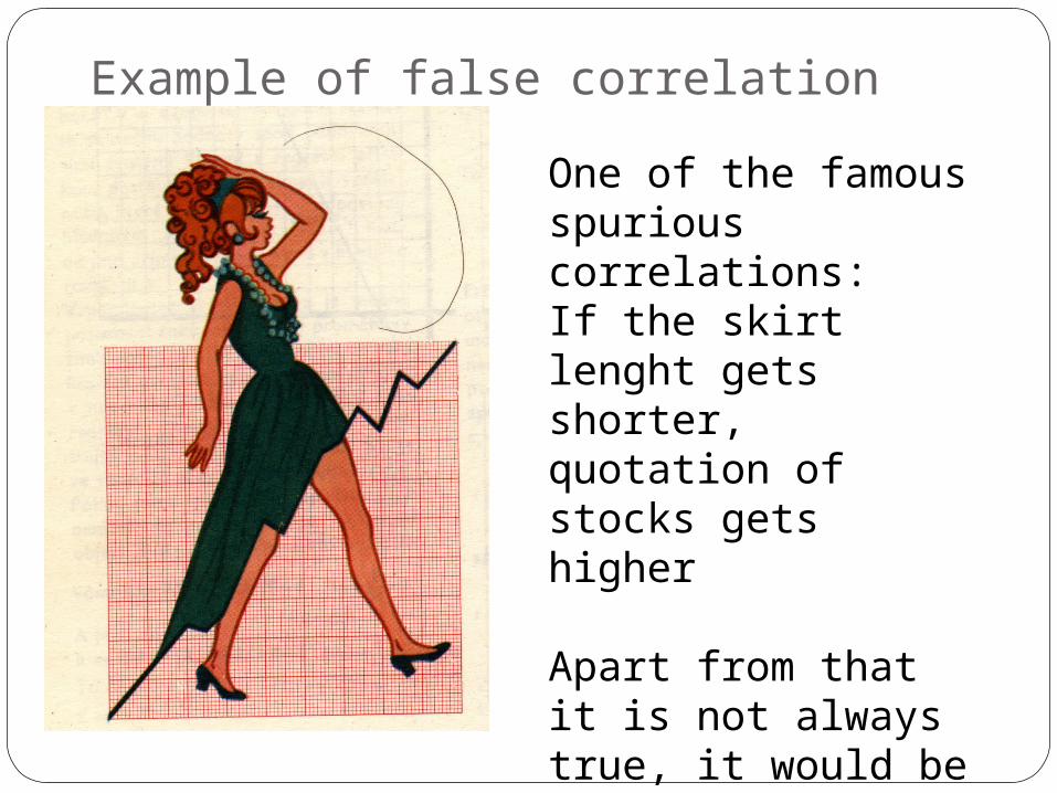
Example of false correlation

5

One of the famous spurious correlations:If the skirt lenght gets shorter, quotation of stocks gets higher

Apart from that it is not always true, it would be false, or spurious correlation.

Examples of statistical - free - dependence

6

Examination how consumption of pork depend on income, price of pig meat, beef, poultry and tradition resp. another unspecified, or random effects.

Examination of dependence of GNP on Labour and Capital...

Ivestigation if the nutrition of the population depend on the degree of economic development of the country

Opposite of the statistical dependence is the functional dependence

7

Y = f(X1 X2…... Xk ,Bo , B1 ,…., Bp)

Where the dependent variable is clearly determined by functional relationship,

Examples from physics, chemistry – this kind of relationship is not the subject of statistical investigation.

Regression and correlation analysis (RaKA)

8

Two basic task of RaKA:Regressiona) find a functional relationship by which

the dependent variable changes with the change of independent variables - find a suitable regression line (function).

b) It is also necessary to estimate the parameters of the regression function.

Correlation - to measure strength of the examined dependence (relationship).

Illustration of the correlation field in two cases (scatter plot)

9

x

yy

x

According to the number of independent variables are distinguished:

10

Simple dependence, when we consider only one independent variable X, we investigate the relationship between Y and X.

Multiple dependence , we are considering at least two independent variables veličiny X1, X2, … Xk , for k 2

Simple regression and correlation analysis

11

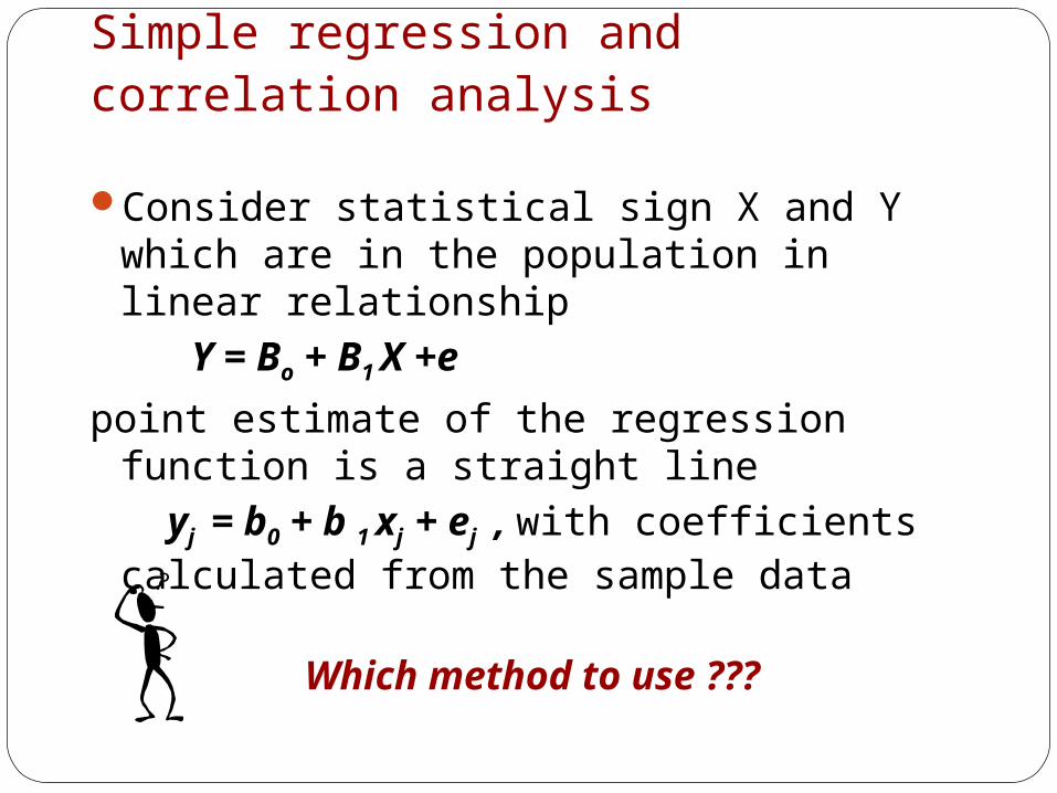
Consider statistical sign X and Y which are in the population in linear relationship Y = Bo + B1 X +e

point estimate of the regression function is a straight line yj = b0 + b 1 xj + ej , with coefficients calculated from the sample data

Which method to use ???

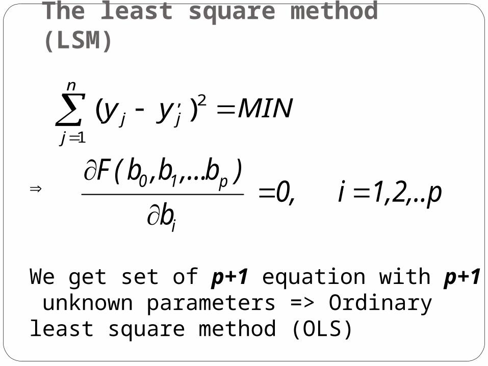
The least square method (LSM)

12

MINyyn

jjj )( 2

1

,

1,2,..p i 0, b

)b,...b,b(F

i

p10

We get set of p+1 equation with p+1 unknown parameters => Ordinary least square method (OLS)

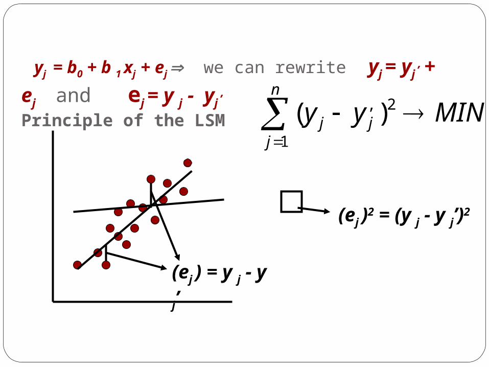
yj = b0 + b 1 xj + ej we can rewrite yj = yj ,

+ ej and ej = y j - yj ,

Principle of the LSM

13

(ej ) = y j - y j’

(ej )2 = (y j - y j’)2

MINyy j

n

jj )( 2,

1

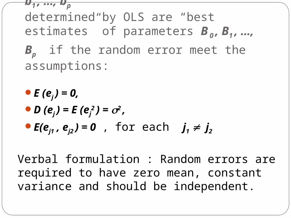
Can be proved that coefficients bo , b1 , …, bp

determined by OLS are “best estimates” of parameters B 0 , B1 , …, Bp if the random error meet the assumptions:

14

E (ej ) = 0,

D (ej ) = E (ej2 ) = 2 ,

E(ej1 , ej2 ) = 0 , for each j1 j2

Verbal formulation : Random errors are required to have zero mean, constant variance and should be independent.

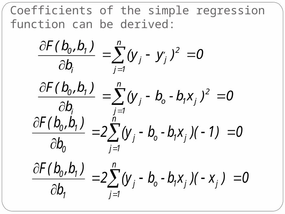
Coefficients of the simple regression function can be derived:

15

0)xb - b(y b

)b,b(F

0)y(y b

)b,b(F

2j1o

n

1jj

i

10

2,j

n

1jj

i

10

0)x)(xb - b(y2 b

)b,b(F

0)1)(xb - b(y2 b

)b,b(F

jj1o

n

1jj

1

10

j1o

n

1jj

0

10

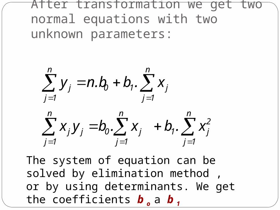
After transformation we get two normal equations with two unknown parameters:

16

n

1j

2j1

n

1jj0

n

1jjj

n

1jj10

n

1jj

x .b x.b yx

x .b n.b y

The system of equation can be solved by elimination method , or by using determinants. We get the coefficients b o a b 1

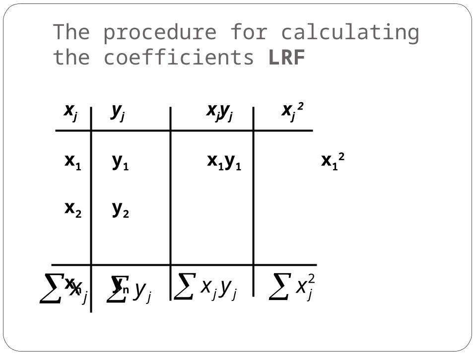
The procedure for calculating the coefficients LRF

17

xj yj xjyj xj 2

x1 y1 x1y1 x12

x2 y2

xn yn jy jx jj yx 2jx

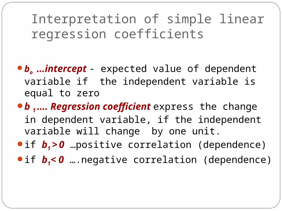
Interpretation of simple linear regression coefficients

18

bo …intercept - expected value of dependent variable if the independent variable is equal to zero

b 1 …. Regression coefficient express the change in dependent variable, if the independent variable will change by one unit.

if b1 > 0 …positive correlation (dependence)

if b1< 0 ….negative correlation (dependence)

Properties of least square method:

19

min )yy( 2n

1j

,jj

01

) y(yn

j

,jj

Regression function passes throught the coordinates a x y

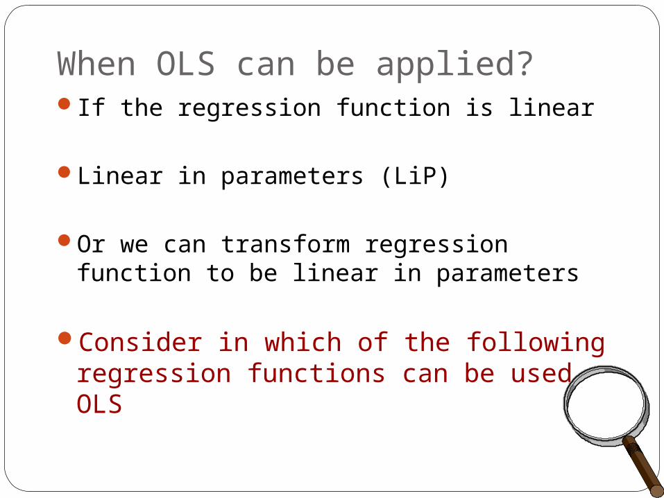
When OLS can be applied?

20

If the regression function is linear

Linear in parameters (LiP)

Or we can transform regression function to be linear in parameters

Consider in which of the following regression functions can be used OLS

Some types of simple regression function:

21

j

j

xoj

bjoj

xoj

jjoj

joj

joj

bbby

xby

bby

xb xbby

xbby

xbby

21'

'

1'

221

'

1'

1'

.

.

. .

log .

/

1

Examples from micro- and macroeconomy

22

Phillips curve ????Cobb -Douglas production curveEngel curvesCurve of economic growthAny other? …...

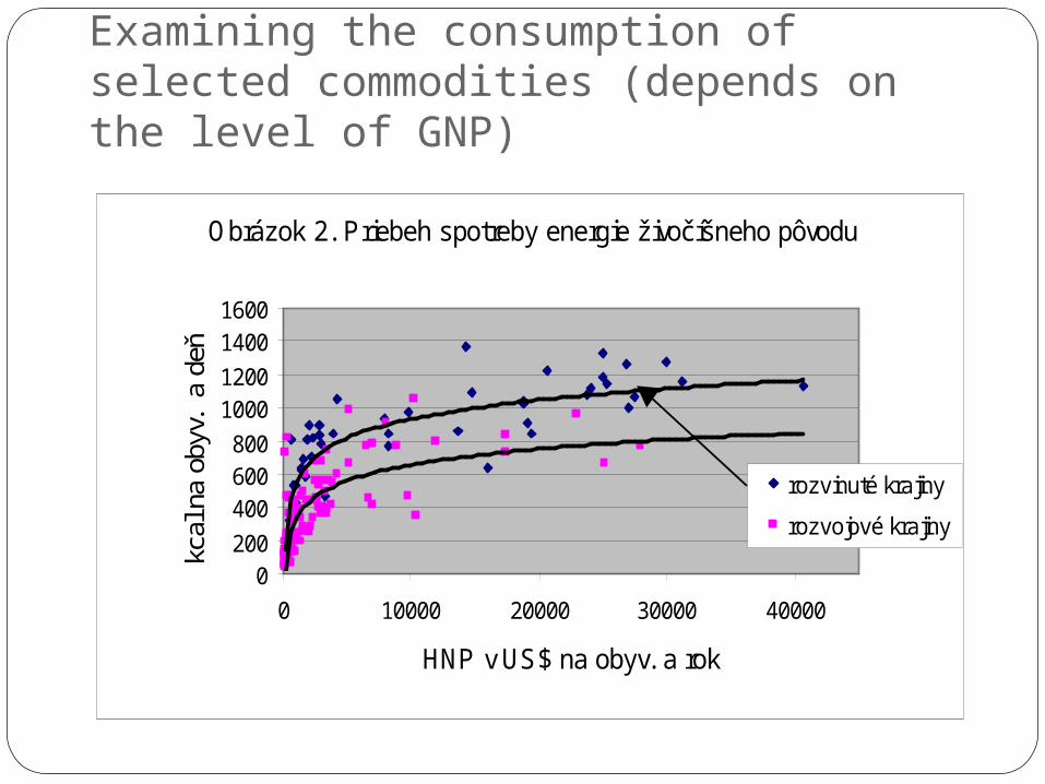
Examining the consumption of selected commodities (depends on the level of GNP)

23

Obrázok 2. Priebeh spotreby energie živočíšneho pôvodu

0200

400600800

10001200

14001600

0 10000 20000 30000 40000

HNP v US$ na obyv. a rok

kcal

na

obyv

. a

deň

rozvinuté krajiny

rozvojové krajiny

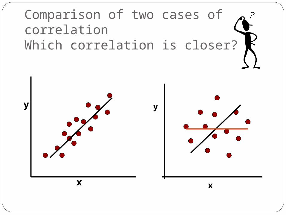
Comparison of two cases of correlationWhich correlation is closer?

24

y

x

y

x

25

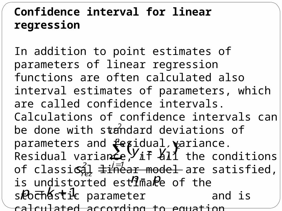
Confidence interval for linear regression In addition to point estimates of parameters of linear regression functions are often calculated also interval estimates of parameters, which are called confidence intervals. Calculations of confidence intervals can be done with standard deviations of parameters and residual variance. Residual variance, if all the conditions of classical linear model are satisfied, is undistorted estimate of the stochastic parameter and is calculated according to equation

pn

yy

s

n

1j

2jj

2rez

1kp

2

26

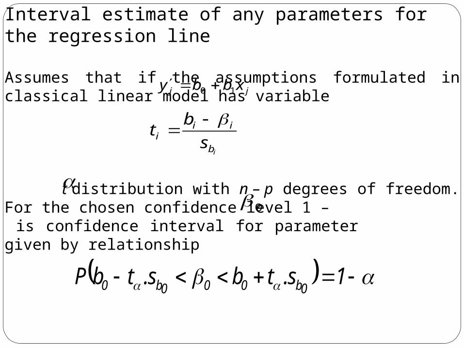
Interval estimate of any parameters for the regression line

Assumes that if the assumptions formulated in classical linear model has variable

t distribution with n – p degrees of freedom. For the chosen confidence level 1 – is confidence interval for parameter given by relationship

jj xbby 10

ib

iii s

bt

0

1s.tbs.tbP0b000b0

27

And for parameter

Analogically is constructed confidence interval for regression line

 

Where is quantile of t distribution S with (for regression line n-2) degrees of freedom.

1

1s.tbs.tbP1b111b1

1s.tyYs.tyPjyjjjyj

2j

r1b )xx(

1.ss

Role of the correlation

28

Examine tightness - strength - of dependence

We use various correlation indicesShould be bounded in intervaland within that interval increased to a

higher power of dependence

29

Correlation analysis provides methods and techniques which are used for verifying of explanatory abilityof quantified regression modelsas a whole and its parts.

Verification of explanatory ability of quantified regression modelsleads to calculation of numerical characteristics,which in concentrated form describe the quality of the calculated models.

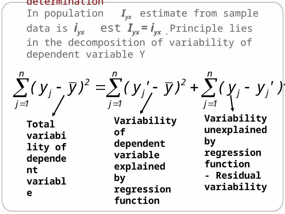
Index of correlation and index of determinationIn population Iyx estimate from sample data

is iyx est Iyx = iyx . Principle lies in the decomposition of variability of dependent variable Y

30

2j

n

1jj

2n

1jj

2n

1jj )'yy()y'y( )yy(

Total variability of dependent variable

Variability of dependent variable explained by regression function

Variability unexplained by regression function- Residual variability

31

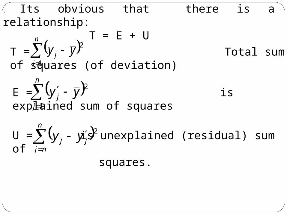
. Its obvious that there is a relationship: T = E + U

T = Total sum of squares (of deviation)

n

jj yy

1

2

E = is explained sum of squares

n

jj yy

1

2

U = is unexplained (residual) sum of squares.

n

njjj yy 2

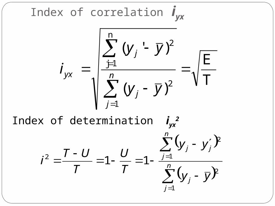
Index of correlation iyx

32

T

E

)(

)'(

2

1

2n

1j

yy

yy

i n

jj

j

yx

Index of determination iyx2

n

jj

n

jjj

yy

yy

T

U

T

UTi

1

2

1

2

2 11

33

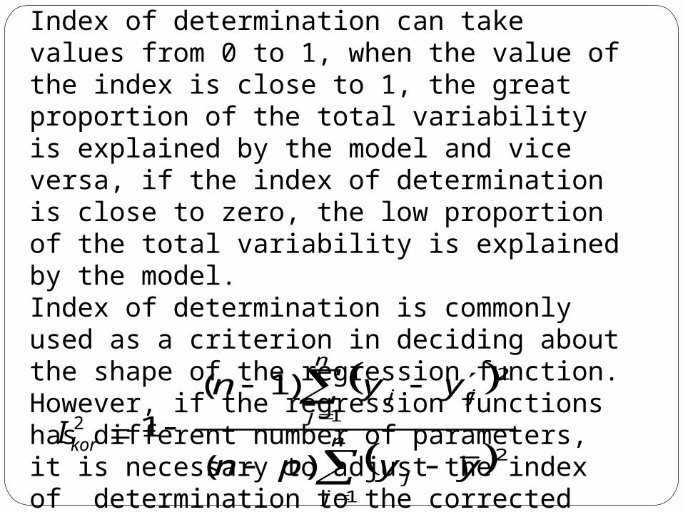
Index of determination can take values from 0 to 1, when the value of the index is close to 1, the great proportion of the total variability is explained by the model and vice versa, if the index of determination is close to zero, the low proportion of the total variability is explained by the model.Index of determination is commonly used as a criterion in deciding about the shape of the regression function. However, if the regression functions has different number of parameters, it is necessary to adjust the index of determination to the corrected form:

2korI

n

jj

n

jjj

yypn

yyn

1

2

1

2

)(

)1(

1

34

n

1j

2j yy

n

njjj yy 2

1p

pn

12

p

Vs y

pn

Nsr

22

2

r

y

s

s

n

jj yy

1

2. 1n

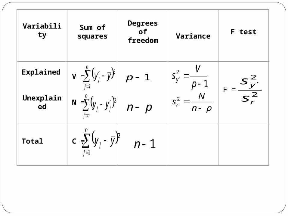
Variability 

Sum of squares

Degrees of freedom Variance

F test

Explained

 Unexplained

V =

N = 

F =

Total C =    

35

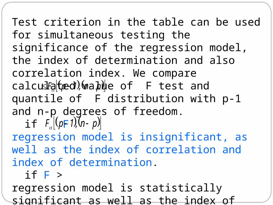
Test criterion in the table can be used for simultaneous testing the significance of the regression model, the index of determination and also correlation index. We compare calculated value of F test and quantile of F distribution with p-1 and n-p degrees of freedom. if F regression model is insignificant, as well as the index of correlation and index of determination. if F > regression model is statistically significant as well as the index of correlation and index of determination.

pn,1pF

pn,1pF

36

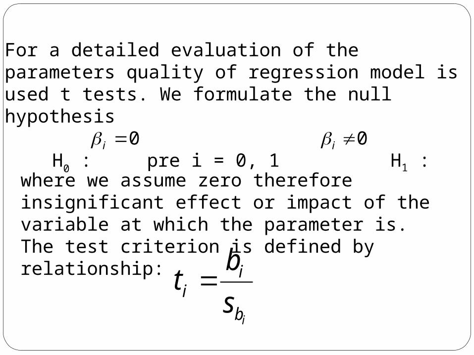
For a detailed evaluation of the parameters quality of regression model is used t tests. We formulate the null hypothesis

H0 : pre i = 0, 1 H1 :0i

where we assume zero therefore insignificant effect or impact of the variable at which the parameter is. The test criterion is defined by relationship:

ib

ii s

bt

0i

37

Where is value of the parameter of regression functionand is standard error of the parameter. 

We will compare calculated value of test criterion with quantile of t distribution at significance level and degrees of freedom .:- if      we do not reject null hypothesis about insignificance of the parameter.-  if       we reject null hypothesis, and confirm statistical significance of the parameter.

ib

ibs

pn

)pn(tt

)pn(tt

38

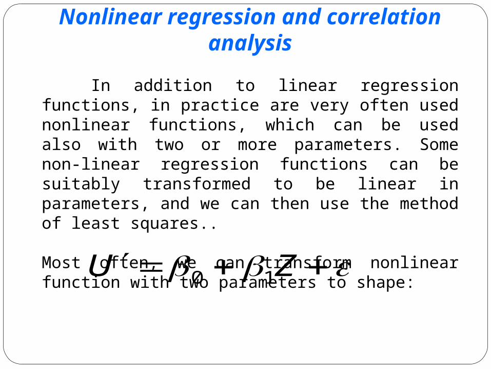
Nonlinear regression and correlation analysis

 In addition to linear regression functions, in practice

are very often used nonlinear functions, which can be used also with two or more parameters. Some non-linear regression functions can be suitably transformed to be linear in parameters, and we can then use the method of least squares.. Most often, we can transform nonlinear function with two parameters to shape:

ZU 10

39

We estimate regression function in form

jj zbbu .10 where

)(yfu )(xfz

Function is then calculated as a linear function. Not all non-linear functions can be converted in this way, only those which are linear in parameters, ie there is some form of transformation called the linearising transformation, most often it is the substitution and logarithmic transformation for example

40

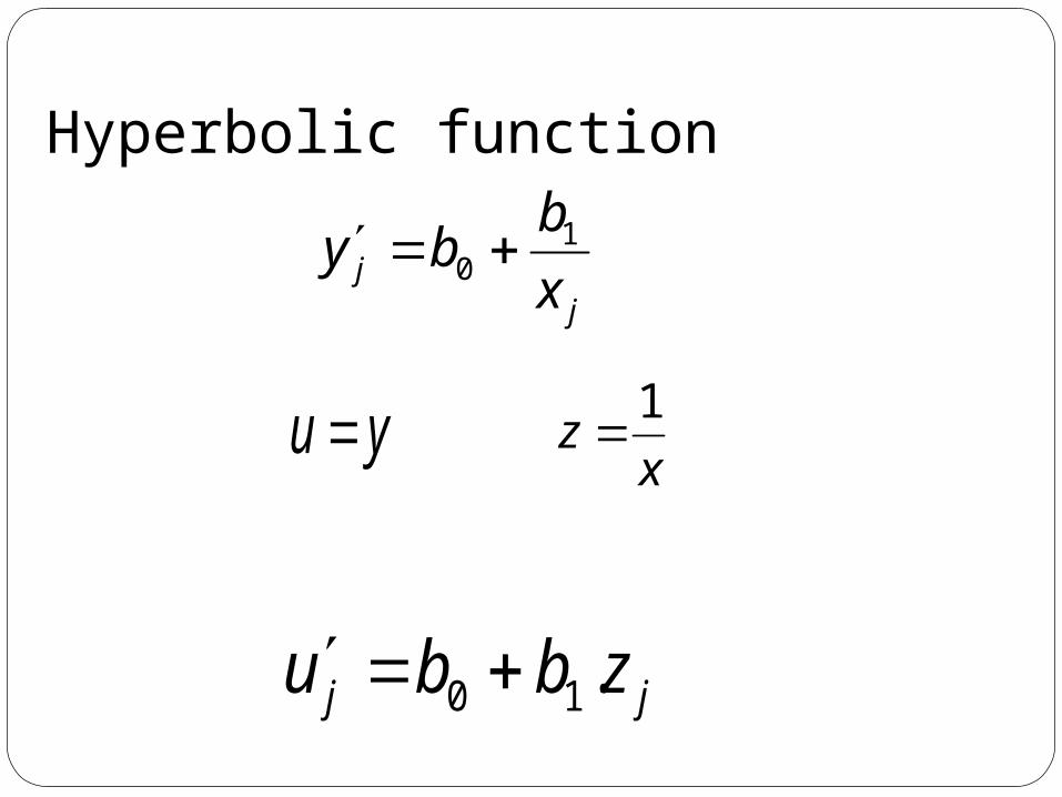
Hyperbolic function

jj x

bby 1

0

yu x

z1

jj zbbu .10

41

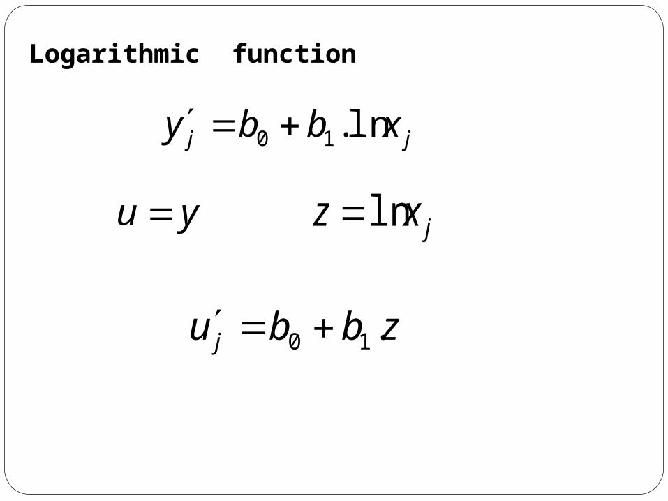
Logarithmic function

jj xbby ln.10

yu jxz ln

zbbu j .10

42

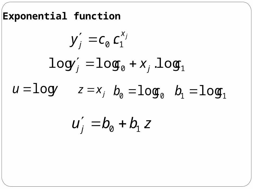
Exponential function

jxj ccy 10 .

10 log.loglog cxcy jj

yu log jxz 00 log cb 11 log cb

zbbu j .10

43

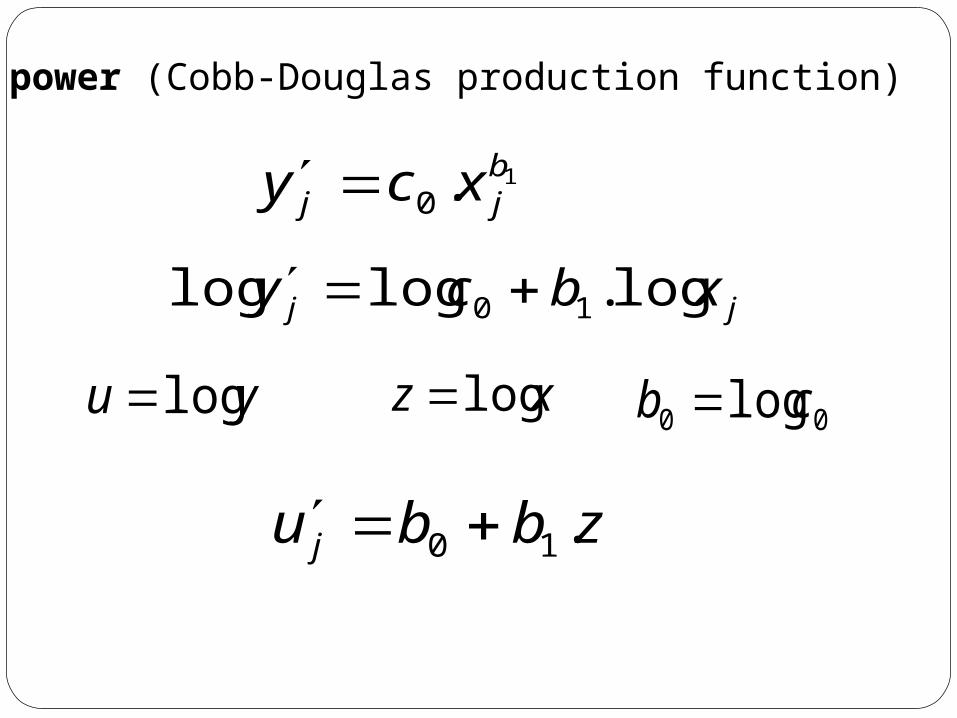
power (Cobb-Douglas production function)

1.0bjj xcy

jj xbcy log.loglog 10

xz logyu log00 log cb

zbbu j .10

44

Similarly, it is possible to modify some more parametrical nonlinear functions such as.second degree parabola

2210 .. jjj xbxbby

2xz

jjj zbxbby .. 210

45

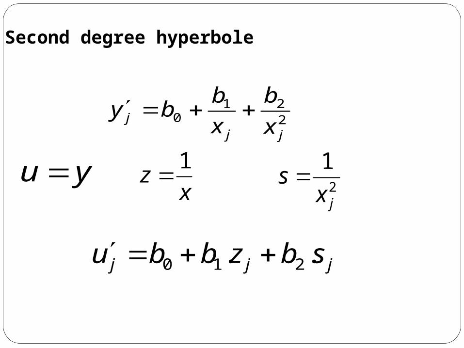
Second degree hyperbole

221

0jj

j x

b

x

bby

yu x

z1

2

1

jxs

jjj sbzbbu .. 210

46

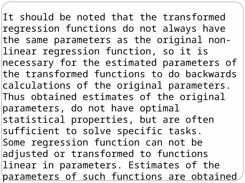
It should be noted that the transformed regression functions do not always have the same parameters as the original non-linear regression function, so it is necessary for the estimated parameters of the transformed functions to do backwards calculations of the original parameters. Thus obtained estimates of the original parameters, do not have optimal statistical properties, but are often sufficient to solve specific tasks.Some regression function can not be adjusted or transformed to functions linear in parameters. Estimates of the parameters of such functions are obtained using different approximate or iterative methods. Most of them are based on so-called gradual improvement of initial estimates, which may be eg. expert estimates, or the estimates obtained by the selected points and so on.

47

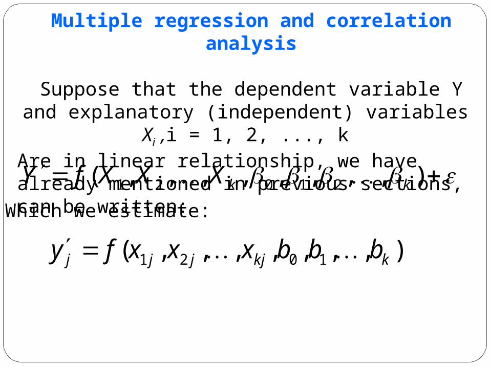
Multiple regression and correlation analysis

Suppose that the dependent variable Y and explanatory (independent) variables Xi ,i = 1, 2, ..., k 

Are in linear relationship, we have already mentioned in previous sections, can be written:

),,,,,,,,( 21021 kkXXXfY Which we estimate:

),,,,,,,( 1021 kkjjjj bbbxxxfy

48

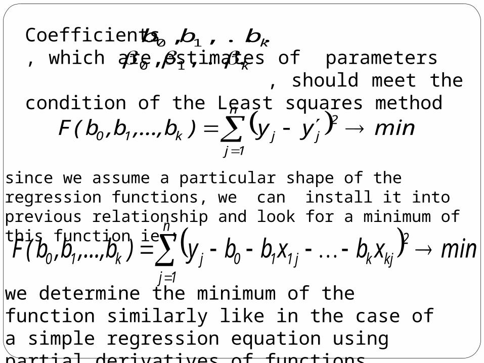
Coefficients , which are estimates of parameters , should meet the condition of the Least squares method

kbbb ,...,, 10

k ,...,, 10

n

1j

2jjk10 minyy)b,...,b,b(F

since we assume a particular shape of the regression functions, we can install it into previous relationship and look for a minimum of this function ie.:

n

1j

2kjkj110jk10 minxbxbby)b,...,b,b(F

we determine the minimum of the function similarly like in the case of a simple regression equation using partial derivatives of functions

49

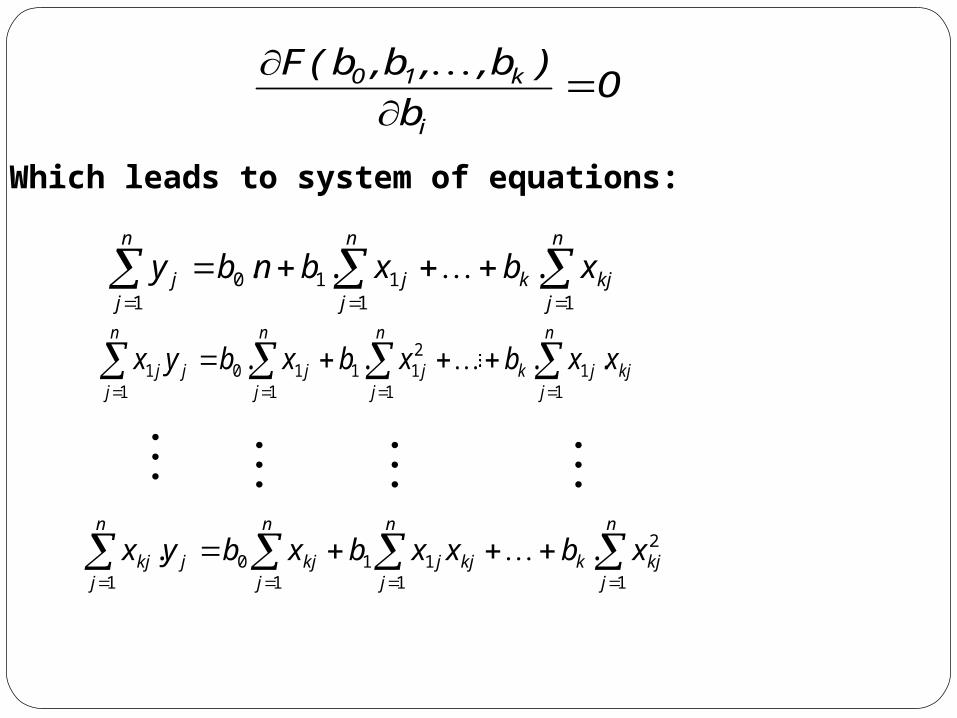
0b

)b,,b,b(F

i

k10

Which leads to system of equations:

n

j

n

jkjk

n

jjj xbxbnby

1 11110 ...

n

jkjjk

n

jj

n

jj

n

jjj xxbxbxbyx

11

1

211

110

11 ....

n

jkjk

n

jkjj

n

jkj

n

jjkj xbxxbxbyx

1

2

111

110 ..

50

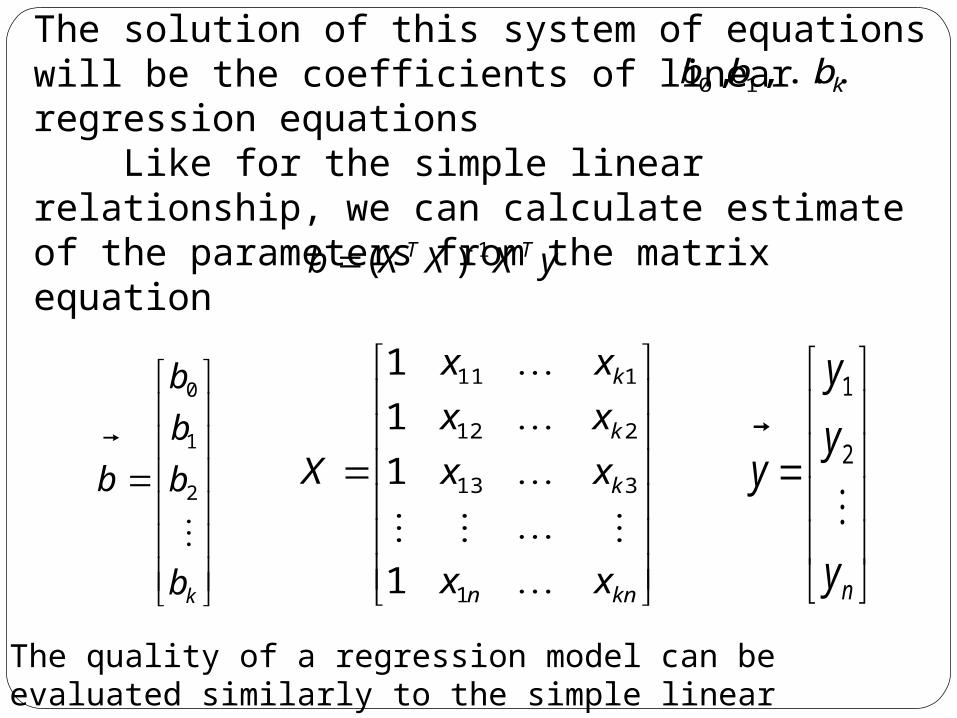
The solution of this system of equations will be the coefficients of linear regression equations Like for the simple linear relationship, we can calculate estimate of the parameters from the matrix equation

kbbb ,...,, 10

yXXXb TT 1)(

kb

b

b

b

b

2

1

0

knn

k

k

k

xx

xx

xx

xx

X

1

313

212

111

1

1

1

1

ny

y

y

y

2

1

The quality of a regression model can be evaluated similarly to the simple linear relationship, which we described in the previous section.

51

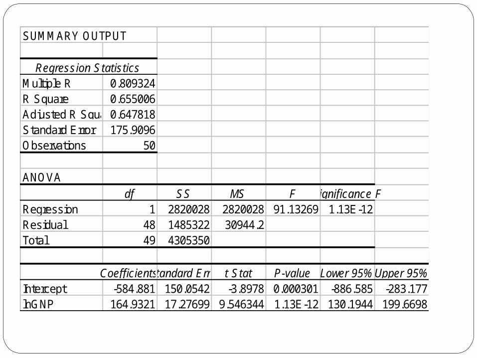
SUMMARY OUTPUT

Regression StatisticsMultiple R 0.809324R Square 0.655006Adjusted R Square0.647818Standard Error 175.9096Observations 50

ANOVAdf SS MS F Significance F

Regression 1 2820028 2820028 91.13269 1.13E-12Residual 48 1485322 30944.2Total 49 4305350

CoefficientsStandard Error t Stat P-value Lower 95%Upper 95%Intercept -584.881 150.0542 -3.8978 0.000301 -886.585 -283.177lnGNP 164.9321 17.27699 9.546344 1.13E-12 130.1944 199.6698

52

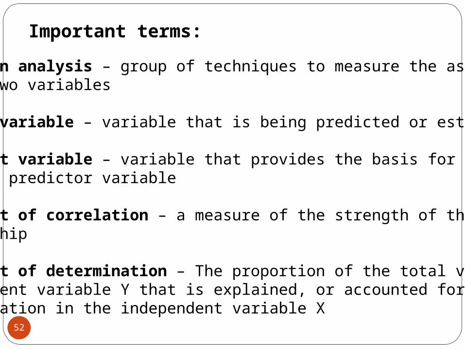
Important terms:

Correlation analysis – group of techniques to measure the association between two variables

Dependent variable – variable that is being predicted or estimated

Independent variable – variable that provides the basis for estimation. It is the predictor variable

Coefficient of correlation – a measure of the strength of the linear relationship

Coefficient of determination – The proportion of the total variation inthe dependent variable Y that is explained, or accounted for, by the variation in the independent variable X

53

Regression equation – An equation that express relationship between variables

Least square principle – Determining a regression equation by minimizing the sum of the squares of the vertical distances between the actual Y values and the predicted values of Y