recent trends in salmon price volatility
TRANSCRIPT

This article was downloaded by: [Northeastern University]On: 22 November 2014, At: 03:14Publisher: Taylor & FrancisInforma Ltd Registered in England and Wales Registered Number: 1072954 Registeredoffice: Mortimer House, 37-41 Mortimer Street, London W1T 3JH, UK
Aquaculture Economics & ManagementPublication details, including instructions for authors andsubscription information:http://www.tandfonline.com/loi/uaqm20
RECENT TRENDS IN SALMON PRICEVOLATILITYAtle Oglend aa Department of Industrial Economics , University of Stavanger ,Stavanger , NorwayPublished online: 19 Aug 2013.
To cite this article: Atle Oglend (2013) RECENT TRENDS IN SALMON PRICE VOLATILITY, AquacultureEconomics & Management, 17:3, 281-299, DOI: 10.1080/13657305.2013.812155
To link to this article: http://dx.doi.org/10.1080/13657305.2013.812155
PLEASE SCROLL DOWN FOR ARTICLE
Taylor & Francis makes every effort to ensure the accuracy of all the information (the“Content”) contained in the publications on our platform. However, Taylor & Francis,our agents, and our licensors make no representations or warranties whatsoever as tothe accuracy, completeness, or suitability for any purpose of the Content. Any opinionsand views expressed in this publication are the opinions and views of the authors,and are not the views of or endorsed by Taylor & Francis. The accuracy of the Contentshould not be relied upon and should be independently verified with primary sourcesof information. Taylor and Francis shall not be liable for any losses, actions, claims,proceedings, demands, costs, expenses, damages, and other liabilities whatsoever orhowsoever caused arising directly or indirectly in connection with, in relation to or arisingout of the use of the Content.
This article may be used for research, teaching, and private study purposes. Anysubstantial or systematic reproduction, redistribution, reselling, loan, sub-licensing,systematic supply, or distribution in any form to anyone is expressly forbidden. Terms &Conditions of access and use can be found at http://www.tandfonline.com/page/terms-and-conditions

RECENT TRENDS IN SALMON PRICE VOLATILITY
Atle OglendDepartment of Industrial Economics, University of Stavanger, Stavanger, Norway
& The price of farmed Atlantic salmon from Norway has increased in recent years. This newregime follows several years of consistently falling prices. At the same time price volatility hasincreased substantially. This article models the volatility of salmon prices and establishes empiri-cally that volatility is on an increasing trend. Further empirical analysis suggests that the volatilitytrend is largely accounted for by the common trend in other food prices relevant to salmon, includ-ing meats, cereals, oils and fish meal observed in recent years. Other potentially contributing factorsto volatility are also discussed. This includes the role of the 2005 maximum total allowable biomassrestriction, the 2006 introduction of the Fish Pool ASA futures market for salmon, the ChileanSalmon crisis and the increasing use of bilateral contracts.
Keywords aquaculture, markets, salmon, volatility
INTRODUCTION
Since the start of intensive salmon farming, salmon has become anincreasingly cheaper source of protein. Salmon has transitioned from arelative luxurious food item to a staple part of everyday diets. For mostof the 1980s and 1990s the price of salmon fell consistently both in nom-inal and real terms. The price decline was caused by steady improvementsin productivity, reducing unit production costs (Asche, 1997, Tveteras &Wan, 2000; Guttormsen, 2002; Vassdal, 2006; Asche et al., 2007; Asche,2008; Asche et al., 2009b). Along with improvements in productivity sal-mon has enjoyed strong demand growth (Asche et al., 2011). However,since the early part of the last decade prices seem to have leveled outand even increased. In some sense demand growth seems to have caughtup with productivity growth. Although productivity still increases itappears to have slowed down relative to demand growth (Vassdal & Holst,2011).
Address correspondence to Atle Oglend, Department of Industrial Economics, University of Sta-vanger, 4036 Stavanger, Norway. E-mail: [email protected]
Aquaculture Economics & Management, 17:281–299, 2013Copyright # Taylor & Francis Group, LLCISSN: 1365-7305 print/1551-8663 onlineDOI: 10.1080/13657305.2013.812155
Dow
nloa
ded
by [
Nor
thea
ster
n U
nive
rsity
] at
03:
14 2
2 N
ovem
ber
2014

This apparent slowdown must also be seen relative to recent developmentsin demand conditions. The Chilean disease issues, starting in late 2008, shifteddemand towards non-Chilean suppliers (Asche et al., 2009a; Hansen &Onozaka, 2011). This provided strong prices for Norwegian salmon farmers.The shock is likely temporary as the Chilean industry seems to be recovering.More importantly overall global growth in demand for food, including pro-tein, has been strong and is likely to remain strong (Trostle et al., 2011). Thissuggests continued high demand for fish, putting continued upward pressureon prices.
Volatility has also increased along with increasing prices. High volatilityis not surprising considering the perishable nature of harvested salmon inaddition to a long production time. This effect is demonstrated in Oglendand Sikveland (2009). Recent developments show a steady increase in pricevolatility. This is different from occasional shocks, or clustering, of volatilityassociated with temporary seasonal effects such as temperature fluctuations(Asheim et al., 2011). Higher volatility is not necessarily bad as farmersappear to be compensated by higher prices in general. For processors, how-ever, extreme price movements might put undesirable pressure on profitmargins. At least it should make hedging instruments more attractive forrisk adverse processors.
Higher prices of proteins have increased the production cost of salmon.Cereals, oils and meals (specifically fishmeal) are important input factors insalmon production. Given a strong demand for fish some of these higherproduction costs can be passed to consumers. Whether strong demandand higher production costs lead to higher price volatility is an importantquestion. There is at least one channel by which this could be the case. Theopportunity cost of harvesting, in essence a cost of storing fish by having tokeep the fish in pens, increases when feed prices increase. Fish notharvested will have to be fed even with little net growth benefits. It is likelythat higher feed prices, in combination with strong current demand forfish, will lead farmers to harvest earlier than they otherwise would. Suchbehavior will lead to less supply smoothing, reducing the short-runelasticity of supply. As a consequence the volatility of prices will increase.
Volatility is important in terms of biomass management. Biomass man-agement refers to decisions concerning harvesting and restocking to keep astanding stock of fish sufficient to meet demand at lowest possible costs.The biological production process is long, leading to slow adjustments toshocks (Andersen et al., 2008). With more price volatility the value of thebiomass becomes more uncertain. This makes managing the biomass moredifficult. In addition returns to investments in the industry become moreuncertain. In terms of salmon price volatility Oglend and Sikveland(2009) demonstrate that price volatility is itself volatile. Solibakke (2012)uses a stochastic volatility model to demonstrate that front month futures
282 A. Oglend
Dow
nloa
ded
by [
Nor
thea
ster
n U
nive
rsity
] at
03:
14 2
2 N
ovem
ber
2014

contracts of salmon display significant time varying volatility. In terms offorecasting salmon prices (Guttormsen, 1999), higher price volatility willincrease the variance of forecast errors. The price risk comes in additionto a substantial production risk (Asche & Tveteras, 1999; Tveteras, 1999;Kumbhakar & Tveteras, 2003).
The purpose of this article is twofold. First, an empirical measure ofsalmon price volatility is established. Using a derived measure of volatility froma GARCH model evidence of strong co-movement between price volatility andglobal food prices is provided. This lends support to a hypothesis that higherprice volatility is due to strong demand and higher production costs. Second,other potential factors influencing volatility such as the 2005 maximum allow-able biomass (MTB) restriction, the introduction of a futures market forsalmon (Fish Pool), the Chilean salmon crisis and the change in use of bilat-eral contracts are discussed. Next, salmon price volatility is defined and pre-liminary evidence of higher price volatility is established. Following thissome potential factors affecting volatility are discussed and an empirical inves-tigation of food prices and volatility is carried out.
THE VOLATILITY OF SALMON PRICE
The price of salmon used in this article is weekly prices paid by expor-ters to Norwegian farmers for fresh gutted salmon of superior quality. Thedata can be found at www.nosclearing.com. Norway is the largest producerof farmed Atlantic salmon with a market share of 50% in 20081 (FAO,2010). Most salmon from Norway is exported, with EU as the primaryexport market. Our observations cover the first week of 1995 to week 37in 2012. Figure 1 shows the prices.
Since the early 2000s, prices have been on an increasing trend with alarge correction towards the end due to the Chilean recovery. In additionto the price we observe greater week-by-week price fluctuations towards theend of the sample.
Volatility can be defined as variations in prices around its expectedvalue. If expected prices are formed as the expected future intersection
FIGURE 1 The nominal price of fresh Atlantic Salmon.
Salmon Price Volatility 283
Dow
nloa
ded
by [
Nor
thea
ster
n U
nive
rsity
] at
03:
14 2
2 N
ovem
ber
2014

of supply and demand, volatility is fundamentally related to unexpectedmovements in supply and=or demand. A commonly used measure of pricevolatility which avoids the specification of an expected price is the standarddeviation of price returns. Volatility is here a measure of the magnitude ofprice fluctuations from period to period.
Figure 2 shows the annual mean price of salmon and the annual stan-dard deviation of weekly price returns (logarithmic)2.
Figure 2 establishes the same stylized fact hinted to in Figure 1—volatilityand price have increased since the early 2000s. A varying volatility is not sur-prising. Salmon is a seasonally produced commodity where most fish growthoccurs in summer=early fall when sea water temperatures are high (Herman-sen & Heen, 2012). As with other seasonally produced commodities, such ascorn or wheat, volatility is greatest just prior to the production or harvest per-iod (Peterson & Tomek, 2005) when annual stocks are lowest. For storablecommodities volatility is decreasing in available stocks. Larger availabilityleads to increased supply elasticity as stocks are used to buffer demand move-ments. In the spring, a convenience yield can arise as expected immediategrowth is high and thus immediate production valuable. The cost of storingand producing (keeping the fish in the pens) might be negative leading tohigher spot prices and lower expected future prices.
This phenomenon is known as ‘‘backwardation’’ in futures markets. Ifbiomass is lower than expected prior to the production period farmers mustbe compensated by higher prices in order to give up the valuable high growthperiod. In such circumstances there is not enough fish to satisfy both con-sumption and ‘‘production’’ demand. If processors and exporters want fishon the spot they must bid up the price. These occasional seasonal spikes, asin for example the spring=summer of 2006, will lead to variation in volatilitybetween years. Unless such seasonal spikes occur with increasing frequency,these effects should be distinguished from long-run trends in volatility.
Another way to examine volatility is to look at the number of price move-ments exceeding a specific level. In the full sample the standard deviation of
FIGURE 2 Annual mean salmon prices (left axis, black) and the standard deviation of log-returns.
284 A. Oglend
Dow
nloa
ded
by [
Nor
thea
ster
n U
nive
rsity
] at
03:
14 2
2 N
ovem
ber
2014
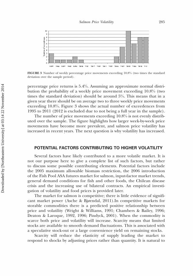
percentage price returns is 5.4%. Assuming an approximate normal distri-bution the probability of a weekly price movement exceeding 10.8% (twotimes the standard deviation) should be around 5%. This means that in agiven year there should be on average two to three weekly price movementsexceeding 10.8%. Figure 3 shows the actual number of exceedences from1995 to 2011 (2012 is excluded due to not being a full year in the sample).
The number of price movements exceeding 10.8% is not evenly distrib-uted over the sample. The figure highlights how larger week-by-week pricemovements have become more prevalent, and salmon price volatility hasincreased in recent years. The next question is why volatility has increased.
POTENTIAL FACTORS CONTRIBUTING TO HIGHER VOLATILITY
Several factors have likely contributed to a more volatile market. It isnot our purpose here to give a complete list of such factors, but ratherto discuss some possible contributing elements. Potential factors includethe 2005 maximum allowable biomass restriction, the 2006 introductionof the Fish Pool ASA futures market for salmon, input-factor market trends,general demand conditions for fish and other foods, the Chilean diseasecrisis and the increasing use of bilateral contracts. An empirical investi-gation of volatility and food prices is provided later.
The market for salmon is competitive; there is little evidence of signifi-cant market power (Asche & Bjørndal, 2011).In competitive markets forstorable commodities there is a predicted positive relationship betweenprice and volatility (Wright & Williams, 1991; Chambers & Bailey, 1996;Deaton & Laroque, 1992, 1996; Pindyck, 2001). When the commodity isscarce both price and volatility will increase. Scarcity means that limitedstocks are available to smooth demand fluctuations. This is associated witha speculative stock-out or a large convenience yield on remaining stocks.
Scarcity will reduce the elasticity of supply leading the market torespond to shocks by adjusting prices rather than quantity. It is natural to
FIGURE 3 Number of weekly percentage price movements exceeding 10.8% (two times the standarddeviation over the sample period).
Salmon Price Volatility 285
Dow
nloa
ded
by [
Nor
thea
ster
n U
nive
rsity
] at
03:
14 2
2 N
ovem
ber
2014

investigate the change in volatility by looking at the scarcity of salmon. Hassalmon become scarcer in recent years?
In terms of salmon from Norway there is little evidence of scarcity if welook at total annual biomass (Figure 4). From the figure we observe a con-sistent increase in biomass from 1995 and onwards. However, total biomassis not a sufficient measure of scarcity as total biomass includes both fishready to harvest (speculative stock) and fish used for further productionthrough growth. It is possible that supply=demand conditions are tighteven if total biomass has increased. For example, if demand from proces-sors and exporters grows, farmers might still be wary to increase their har-vests too much so as not to sacrifice future biomass3.
One factor deserving of discussion here is the Chilean salmon crisis.Starting in late 2007 the Chilean salmon industry experienced severe diseaseissues (Asche et al., 2009a). This had a significant effect on production from2009 until at least early 2011. From 2011 production appears to at least par-tially recover. To show one effect of the Chilean crisis, Figure 5 shows importsof frozen and fresh filets from Chile and Norway to the United States.
Although imports from Chile decreased substantially, imports fromNorway increased. Norway experienced a positive demand shift. The crisiscan account for the strong prices in 2009 and 2010. From 2011 the importmarket appears to be normalizing. The positive demand shift for Norwe-gian salmon contributed to the relative scarcity of salmon, and has likelycontributed to keeping volatility high. However, the general increase involatility started from around 2005, four years before the Chilean crisis.
The Maximum Total Allowable Biomass Restriction
Prior to 2005 salmon farmers in Norway faced restrictions on bothproduction volume per license, biomass density and feed usage (Asche &Bjørndal, 2011). In an attempt to simplify this system a single maximum
FIGURE 4 Total annual salmon biomass from 1995–2010. Source: Norwegian Directorate ofFisheries (2012).
286 A. Oglend
Dow
nloa
ded
by [
Nor
thea
ster
n U
nive
rsity
] at
03:
14 2
2 N
ovem
ber
2014

total allowable biomass restriction (MTB) was introduced in 2005. TheMTB restriction states that a farmer can keep no more than 65 tons of fishper 1,000 m3 license volume. A standard license (12,000 m3) is then con-verted to 780 tons MTB. Based on the number of licenses and the standardlicense size, we can construct a crude measure of capacity utilization in theindustry.4
Figure 6 shows MTB-implied capacity utilization from 1995 to 2010.According to this measure capacity utilization has increased steadily sincethe start of the sample. In 2010 capacity utilization was over 81%. Thismight be an indication that supply=demand conditions have become tigh-ter in recent years. This suggests that higher price volatility is linked to tigh-ter supply=demand conditions for Norwegian farmers and an effectivescarcity of fish. Of course this is a simple correlation and not evidence ofcausality so we should remain skeptical and look for other corroborativeevidence.
FIGURE 5 U.S. imports of Atlantic salmon from Chile and Norway. Source: NOAA (2013).
FIGURE 6 MTB implied capacity utilization for Norwegian salmon farms. Note: Available capacity is cal-culated as (number of licenses� average license’s MTB). The average license’s MTB is 780 tons of sal-mon. Capacity utilization is then estimated as the average total biomass’ share of available capacity.Source: Norwegian Directorate of Fisheries (2012).
Salmon Price Volatility 287
Dow
nloa
ded
by [
Nor
thea
ster
n U
nive
rsity
] at
03:
14 2
2 N
ovem
ber
2014

At least from a theoretical standpoint an MTB-type restriction is likelyto affect harvest patterns. If farmers expect capacity to be binding theyare likely to harvest earlier than planned and thereby creating larger fluc-tuations in harvests. The direct consequence of violating MTB restrictionsare fines equal to the amount (in kg) exceeding MTB times a relevant salesprices set by the Norwegian Directorate of Fisheries. Violations of MTB arebased on self-reported biomass. There is anecdotal evidence that if MTB islikely to be binding a certain month farmers will increase harvest prior tothe end of the relevant month. This is because they have to report at thestart of each month the prior month biomass. MTB has been binding forfarms in recent years as companies have been fined in accordance with reg-ulations due to MTB violations.
It should be noted that effective biomass restrictions were in place priorto the current MTB regime. The stated purpose of the current MTB regimewas to simplify reporting and give individual farmers more flexibility.Hence, the changes in regulations can, but need not have contributed toincreased volatility.
Hedging Instruments
From May 2006 futures contracts for salmon have been traded on aderivative market facilitated and organized by Fish Pool ASA (www.fishpoo-l.eu) in collaboration with NOS clearing. This market has provided newhedging instruments outside of the traditional bilateral agreements. Inaddition to hedging and risk sharing, the futures market can provide neces-sary standardization and price discovery regarding the value of salmon. Ifmarkets are liquid and otherwise well-functioning, derivatives could pro-vide stabilizing effects on prices through improved conditions for biomassand marketing decisions. Alternatively, if futures prices are consistently‘‘wrong,’’ and spot prices are affected by futures prices, the introductionof the futures market could add unnecessary price volatility.5 An additionalproblem could arise if relatively little volume is traded on the futures mar-ket but other market agents use futures prices for biomass and marketingdecisions.
If we are to take volume as an indication, it is unlikely that the futuresmarket has had much effect on the spot price of salmon. Although tradedvolume on the futures market has consistently increased (31,700 tons salmonequivalence in 2007 to 100,630 tons in 2010)6, it is still relatively small com-pared to the total size of the market. It is still possible for futures prices toaffect spot prices given enough agents make decisions based on futures priceswithout participating directly in the market. To examine this effect furthernecessitates a detailed empirical study outside the scope of this article.
288 A. Oglend
Dow
nloa
ded
by [
Nor
thea
ster
n U
nive
rsity
] at
03:
14 2
2 N
ovem
ber
2014
Of specific relevance to price volatility is the use of bilateral contracts tohedge cash-flows. With salmon becoming a staple item at retail stores acrossEurope a steady supply of fish is demanded. As such bilateral agreementshave become more prevalent in recent years (Kvaløy & Tveteras, 2008; Lar-sen & Asche, 2011). Increasing use of bilateral agreements over spot trad-ing is relevant as it affects short-run supply elasticity. If more biomass is tiedto binding contracts then less fish is available to respond to short-rundemand fluctuations. This effectively means that less ‘‘speculative’’ stockis available. Even if farmers expect higher prices they could not respondby delaying harvests as fish is tied to contracts. This will have the directeffect of increasing short-run price volatility.
General Food Price Trends
Food prices on a global scale have been strong in recent years. Variousfactors have contributed to this. Increasing energy prices, the bio-fuel rev-olution, a weak dollar, export restrictions and rapid economic growth,specifically in China and India, combined with low yields are some pro-posed factors explaining the price run-up (Minot, 2010; Baffes, 2011).Especially relevant to fish is the ‘‘westernization of diets’’ from consumersexperiencing rising purchasing power. This has resulted in increasingdemand for protein and more varied diets in general (Zhang & Law, 2010).
In addition to increasing prices, the so-called biofuel revolution has cre-ated new connections between agriculture and energy markets (Serra et al.,2010; Ciaian & Kancs, 2011; Nazlioglu and Soytas, 2011; Salvo & Huse,2011). This has directly manifested in a stronger relationship between cornand ethanol prices and, by extension, gasoline (Du & Lu McPhail, 2012).Energy has always been an important factor on the input side of agricul-tural production but has only recently become a substitute to energy onthe demand side. This has caused stronger volatility spill-over effects fromenergy to agricultural markets in recent years (Trujillo-Barrera et al., 2011).
Salmon is related to other commodities both through food substitutionand input factors, because salmon aquaculture feed accounts for the largestshare of production costs. The major components of salmon feed arefish-meal, fish-oil and soybean-meal. The markets for these important com-modities have not been immune to recent trends in commodity markets. Assuch salmon has experienced both increasing demand and higher pro-duction costs.
Figure 7 illustrates the recent run-up in agricultural prices relevant tosalmon. This includes a meat price index, a cereals price index, an oilsprice index and a capture fish price index7. Meat and capture fish areprotein substitutes for salmon. Cereals, oils and fish-meal are important
Salmon Price Volatility 289
Dow
nloa
ded
by [
Nor
thea
ster
n U
nive
rsity
] at
03:
14 2
2 N
ovem
ber
2014

components in salmon feed. The overall trends for the indices point in thesame direction, with oils and cereals being the most volatile. To investigatethe co-movement in indices we perform a principal component analysis.Table 1 reports the correlation matrix and the variations in indicesaccounted for by the principal components.
A majority of the variation in indices (89.54%) can be accounted for bythe first factor. Examining this factor it accounts for the major long runswings in indices. We will refer to this factor as the food price trend(fpt). Later this factor will be used to examine how volatility correlates withrelevant food prices.
Strong demand for fish and meat in general likely also includes salmon.The 2008 food crisis, which manifested strongly in cereal prices, did notmanifest strongly in aquaculture prices. Capture prices on the other handdid increase significantly up to the summer of 2008. This could be explainedby the stronger energy component in the 2008 crisis. Fuel price is a largercomponent of the direct input cost in capture fisheries. Many of the samefactors contributing to the 2008 commodity price peak also contributedto the recent 2011 food crisis. Contrary to 2008, the 2011 prices hasa stronger meat component (Trostle et al., 2011). Global per capita pork
FIGURE 7 FAO food price indices. Note: 2002–2004¼ 100. The Meat Index contains four types ofmeats: two poultry products, three bovine meat products, three pig meat products and one ovine meatproduct. The Cerals Index contains various grains and rice prices, including wheat and corn. The OilsIndex consists of 12 different oils including animal and fish oils. The Fish Price Index consist of importprices for major fish species traded.
TABLE 1 Correlation Matrix and Principal Components of Food Indices
Meats Cereals Oils Fish Eigenvalues % variation % cumulative
Meats 1 PC1 3.582 89.54 89.54Cereals 0.89 1 PC2 0.192 4.81 94.35Oils 0.84 0.91 1 PC3 0.157 3.94 98.29Fish 0.81 0.88 0.82 1 PC4 0.0683 1.71 100.00
290 A. Oglend
Dow
nloa
ded
by [
Nor
thea
ster
n U
nive
rsity
] at
03:
14 2
2 N
ovem
ber
2014

and poultry consumption has increased steadily the over last decade. Pro-duction decisions (for pork and beef) made when prices were low, followingthe late 2008 price drop, affected supply in 2011, causing higher prices(Trostle et al., 2011). More intensive feeding systems (especially for cattle)with more use of grain and protein meal in combination with high cerealand meal prices has also contributed to upward pressure on meat prices.
Important feed factors like cereals, oils and meal prices have also beenconsistently high. It should be noted that dependence on costly marine pro-teins in aquaculture production has decreased. This decrease is most dramaticfor carnivore’s species such as salmon. The fish-in fish-out ratio for salmondecreased from 7.5 to 4.9 from 1995 to 2006 (Tacon & Metian, 2008). Relativedifferences in protein and cereal prices will trigger substitution on the inputside of production. However, a common trend in input factor prices will limitsubstitution benefits such that production costs have likely increased overall.
Judging by the overall developments in food and feed factor prices, sal-mon has experienced both increasing demand and higher costs of pro-duction in recent years. Salmon competes with other protein sources andis dependent on other agricultural commodities as inputs to production.Will strong demand in addition to higher production costs lead to morevolatile prices? The largest cost component in salmon production is feed(Guttormsen, 2002). Fish not harvested and sold will have to be fed evenwith little net growth benefits. The alternative cost of harvesting, in essencea cost of storing, increases when feed prices increase.
Coupled with strong demand and high prices, it is likely that suchconditions will lead farmers to harvest earlier than they would otherwisedo. Rather than keeping fish in pens and speculating on future price devel-opments, farmers might rather harvest now. Such behavior will lead to lesssupply smoothing, in effect reducing the elasticity of supply. This willincrease the volatility of prices. In the next section, I derive a time-varyingmeasure of volatility and investigates empirically how measurable quantitiessuch as prices directly correlate with salmon price volatility.
Salmon Price Volatility and Food Prices
Here the variance of period-to-period price movements is modeled bya GARCH model (Bollerslev, 1986). In the GARCH model, the currentperiod variance is a function of lagged variances and squared model predic-tion errors. The GARCH model is applied to allow volatility of prices,measured as the standard deviation of non-predictable price movements,the freedom to change in time. Non-predictable price movements are heredefined as the part of prices not accounted for by a predefined parametricmodel of prices. To model current price we use an error correction model.The information set available to predict prices is lagged prices.
Salmon Price Volatility 291
Dow
nloa
ded
by [
Nor
thea
ster
n U
nive
rsity
] at
03:
14 2
2 N
ovem
ber
2014

We will also allow deterministic seasonality. The degree to which themodel error is non-predictable can be evaluated using conventional testsof the i.i.d. nature of model errors such as the Q-statistics. Non-predictableshould here be interpreted relative to the family of univariate linear errorcorrection models and the restricted information set used. The model isnot necessarily an optimal forecasting model or a representation of themarkets true expectations of prices. We will model both week-by-weekand month-by-month volatility of prices, where monthly prices areconstructed as average within month weekly prices.
We denote the logarithm of current price as pt and price return asDpt¼ pt� pt� 1. Current period price return is modeled as:
Dpt ¼ lþ seast þ c0pt�1 þXk
i¼1ciDpt�i þ rtet ; ð1aÞ
r2t ¼
Xm
l¼1ale
2t�l þ
Xp
n¼1bnr
2t�n: ð1bÞ
Equation (1a) is an error correction representation of prices where0> c0>� 2 implies mean reverting prices. If c0¼ 0, prices contain a randomwalk component and do not settle at a stationary distribution. The purpose ofEquation (1a) is to decompose price return into a predictable and non-predictable component. The variation in the non-predictable model error,et, can then be interpreted as the volatility of prices. Due to the possibilityof deterministic seasonality we introduce a deterministic seasonal componentseast in Equation (1a). For the weekly prices we model seasonality by Fourierseries; that is, sums of trigonometric functions. We allow annual, semi-annualand quarterly cycles in the Fourier representation8. For the monthly pricesseasonality is modeled by monthly dummy variables. Experimenting withdifferent cycle frequencies in the Fourier representation suggests thatthe GARCH parameter estimates are robust to the seasonal representation.
The model error et is assumed IID(0,1) such that the implied conditionalvariance of returns is r2
t . The conditional variance is modeled as followinga GARCH process (1b). In the GARCH model the persistence of varianceshocks are dictated by the magnitude of ai and bi in equation (1b). Coefficientsequal to zero implies a constant conditional variance. For a GARCH(1,1)model, where both squared residuals and conditional variance are lagged byone period, the half-life of a shock is ln 0:5ð Þ=ln a1 þ b1ð Þ. The closer a1þ b1
is to unity the longer it takes for a shock to variance to be absorbed.For the weekly series the lag length of differences is set to three weeks;
for the monthly series, two months. These are sufficient to eliminate signifi-cant serial correlation when evaluated by the Q-statistics. Experimentationshows that GARCH parameters are robust to changes in different lagcombinations. For the variance process one period lags for both the squared
292 A. Oglend
Dow
nloa
ded
by [
Nor
thea
ster
n U
nive
rsity
] at
03:
14 2
2 N
ovem
ber
2014

error and variance is sufficient to account for ARCH effects and autocor-relation in squared residuals. The model is estimated by maximum like-lihood. In addition we use variance targeting in the estimation such thatthe conditional variance implied by Equation (1b) is consistent with theunconditional variance of the data (Mezrich & Engle, 1996). Estimationresults for weekly and monthly prices are shown in Table 2.
To make the table more readable the seasonal estimates are not shownbut results are available by request. If we impose a restriction of no deter-ministic seasonality we get a P-value< 0.001 for both the weekly andmonthly model. This suggests the presence of deterministic seasonality.The seasonal effects are not pursued in any greater detail here as it wouldextend beyond the scope of the article. Seasonality in this article is relevantto the degree that it affects volatility. Trying different specifications for sea-sonality (more or less cycles in the Fourier representation) suggests that theGARCH estimates are robust to the imposed seasonality.
The sign of c0 in both models is negative, suggesting mean reversion.Due to the non-standard distribution of c0 under the null (c0¼ 0) theseP-values should be evaluated relative to the Dickey Fuller distributions.The t-statistics of c0 for the weekly and monthly series is �2.134 and�2.343, respectively. Using Dickey Fuller critical values from the relevantnull model (5%¼�3.43, 1%¼�4.01) we cannot reject a unit root in pricelevels. This is in accordance with what is commonly found in the literature(Asche et al., 2002; Tveteras & Asche, 2008; Nielsen et al., 2009).
Both the weekly and monthly GARCH estimates give strong evidenceagainst constant volatility. The coefficients for the ARCH and GARCH
TABLE 2 GARCH Estimation Results
Weekly Prices Monthly Prices
Estimate P-value Estimate P-value
l 0.0541 0.035 l 0.4174 0.019c0 �0.0171 0.033 c0 �0.1183 0.038c1 0.0295 0.484 c1 0.2427 0.018c2 �0.1613 <0.001 c2 0.0565 0.508c3 �0.1176 0.002 a1 0.0431 0.038a1 0.1444 0.002 b1 0.9450 <0.001b1 0.8231 <0.001
P-value P-valueQ(20) – residuals 0.2059 Q(20) – residuals 0.2262
Q(20) – squared res. 0.0797 Q(20) – squared res. 0.0791ARCH (1–5) 0.5051 ARCH (1-5) 0.5204
Note: The Q-statistic is the Box-Pierce test for the null of no-remaining residual autocorrelation. Lagsare given in parenthesis. The Q-statistic is v2(nlags) distributed under the null, where. The ARCH stat-istic is Engle’s LM ARCH test for presence of residual ARCH effects. The test regresses squared residualson own lags and tests for significant coefficients using the F(nlags,nobs-nlags) distribution.
Salmon Price Volatility 293
Dow
nloa
ded
by [
Nor
thea
ster
n U
nive
rsity
] at
03:
14 2
2 N
ovem
ber
2014

terms (a1 and b1) are significantly different from zero. The sums of thecoefficients are close to unity (0.967 for the weekly estimates and 0.988for the monthly series) suggesting strong persistence in volatility shocks.This is not surprising considering the previous investigation of volatility.The implied standard deviations (defined as volatility) from the GARCHestimates for the weekly and monthly series are shown in Figure 8.
Volatility for both the weekly and monthly series suggests a trending ser-ies consistent with what was established earlier. The weekly series showgreater short-run fluctuations since week-by-week fluctuations have beenaveraged out in the monthly series.
If we look at volatility the long-run trend is similar to the trend in foodprices (Figure 7). If we include the implied monthly volatility from theGARCH estimation in the principal component analysis of indices we findthat the first principal component still accounts for most of the variationacross series (87.15%). The correlation between series and the principalcomponents contribution to variance is shown in Table 3. In the principalcomponent analysis excluding volatility (Table 1) the first principal compo-nent accounted for 89.54% of the variation in series. The relatively smalldecrease in explanation from 89.54% to 87.15% by including volatilitysuggests strong co-movement in food prices and volatility.
FIGURE 8 Implied volatility (conditional standard deviations) from GARCH model estimates of weekly(top) and monthly (bottom) price returns.
294 A. Oglend
Dow
nloa
ded
by [
Nor
thea
ster
n U
nive
rsity
] at
03:
14 2
2 N
ovem
ber
2014

This result indicates that the food price trend (fpt) found in the firstprincipal component analysis (Table 1) accounts for much of the trendingin volatility. An OLS regression of the monthly GARCH implied volatility onan intercept and the food price trend (rt¼ b0þ b1fptt) gives an R2 of 0.73.The fit of this regression is shown in Figure 9.
Of course we should be careful in equating this high R2 to a ‘‘true’’relationship between the variables. Both series are highly trending andthe fit could simply be the result of a spurious correlation. To examine thishypothesis further we work under the null hypothesis that the high R2 is theresult of a spurious regression. We generate 50,000 random walk ‘‘food pricetrends’’. Any high R2 as a result of running the regression with these artificialfood price trends will be the result of regressing two highly trending seriesagainst each other. Evaluating the original R2 of 0.73 relative to the R2
distribution from the artificial series we get a P-value of 0.022. As such ouroriginal result indicates a statistically significant positive relationshipbetween food prices and volatility different from a spurious correlation.
One commodity of special relevance to salmon is fishmeal (Asche et al.,2012). Fish meal is a major component in salmon feed and couldpotentially have an effect on salmon price volatility outside of the generalfood price effect established here. The fish-meal price used in this analysisis the monthly CIF price of Peruvian Fish Meal Pellets, 65% protein, fromthe World Bank. Peru is the largest producer of fishmeal, of which almost
FIGURE 9 OLS fit of monthly volatility from GARCH estimation (solid line) on the food price trend(dotted line).
TABLE 3 Correlation Matrix and Principal Components of Food Indices and Volatility of SalmonPrices
Meats Cereals Oils Fish Vol. Eigenvalues % variation % cumulative
Meats 1 PC1 4.357 87.15 87.15Cereals 0.89 1 PC2 0.257 5.15 92.29Oils 0.84 0.91 1 PC3 0.178 3.58 95.87Fish 0.81 0.88 0.82 1 PC4 0.147 2.94 98.81Vol. 0.81 0.79 0.79 0.83 1 PC5 0.059 1.19 100.00
Salmon Price Volatility 295
Dow
nloa
ded
by [
Nor
thea
ster
n U
nive
rsity
] at
03:
14 2
2 N
ovem
ber
2014

all is exported. Fish Meal prices depend on several factors including the ElNino weather phenomenon affecting total catches. High demand forfishmeal for various feeds (aquaculture and non-aquaculture production),including demand from new emerging aquaculture producers such asshrimp farmers in Vietnam, is likely keeping prices of fishmeal high.
The food price trend, accounting for the major swings in food prices,accounts for about 61% of the variation in fishmeal prices. The questionis if controlling for the food price trend, will fish-meal prices have anadditional association with salmon price volatility? We adjust volatility andfish-meal price as rrt ¼ rt � b0 � b1fptt and cfmfmt ¼ fmt � b0 � b1fptt , whereb0 and b1 are estimated by OLS. Both the adjusted series reject a unit rootusing a conventional ADF test at the 1% level. We also include the NOK=EURO exchange rate and the Norwegian Interest Rate (the 1-monthNorwegian Inter Bank Offer Rate) to account for other possible macroeco-nomic effects. Both these variables are defined in growth rates to avoidspurious regression effects. We perform the regression:
rrt ¼ b0 þ b1cfmfmt þ b2exchange ratet þ b3interest ratet þ ut ;
where ut ¼Pk
i¼1 aiut�i þ et is an auto-regressive error and et is assumedIID(0,1). We account for serial correlation directly through a kth orderautoregressive error. Lag length is selected sufficient to eliminate residualautocorrelation. As an alternative to the autoregressive least squares wecould perform ordinary OLS and adjust standard errors non-parametricallyusing the procedure of (Newey & West, 1987). This is the HACSE esti-mation and the results of both procedures are shown next.
As Table 4 shows, there is some evidence that higher fish-meal prices areassociated with higher salmon price volatility although the effect does notappear very strong. Exchange rate and Interest rate effects are even weaker.
The result from this discussion show that a higher volatility of salmonprices is linked to higher food prices in general. This includes both
TABLE 4 Effect of Fish-Meal Price on Salmon Price Volatility
Autoregressive Least Squares Estimation HACSE Estimation
Variable Coefficient t-stat Variable Coefficient t-stat
Constant �0.00029 �0.27 Constant �0.00037 �0.62Fish Meal 0.00679 2.36 Fish Meal 0.01077 2.94Exchange rate growth 0.02406 1.21 Exchange rate growth 0.0165 1.55Interest rate growth 0.00500 1.74 Interest rate growth �0.0096 �0.20Residual AR(1) term 0.8776 11.7Residual AR(2) term �0.0333 �0.34Residual AR(3) term 0.2591 2.60Residual AR(4) term �0.2384 �3.13
296 A. Oglend
Dow
nloa
ded
by [
Nor
thea
ster
n U
nive
rsity
] at
03:
14 2
2 N
ovem
ber
2014

demand side substitutes for salmon such as other meats and fish in additionto important input factors such as cereals, oils and fish-meal. This providessupport for the hypothesis that higher volatility is due to strong demand forsalmon in combination with higher production costs. Fish meal alsoappears to have an additional weak positive association with volatility.
CONCLUSION
This article focuses on recent trends in salmon price volatility. It is demon-strated empirically that volatility of Atlantic salmon from Norway has been onan increasing trend since the start of the 2000s. This is established parametri-cally by modeling conditional variance of price returns by a GARCH model.
Having established this stylized fact the question of why volatility hasincreased is pursued. From commodity price theory the positive associationbetween price and volatility could be explained by tight supply=demand con-ditions. Such tight conditions means that demand fluctuations, in lack ofavailable biomass, must be adjusted by price movements rather than supplyadjustments. Potential factors contributing to tighter supply=demand con-ditions and lower short-run supply elasticity are: 1) strong demand for salmonfrom Norway, partially contributed by the Chilean disease issues, 2) increasedcapacity utilization as a response to favorable demand conditions and theresulting effects of occasionally binding MTB restrictions, 3) the increasinguse of bilateral contracts over spot trading and 4) the overall strong pricesfor relevant commodities globally increasing production costs and contribu-ting to strong demand for salmon. This last factor is given empirical supportby investigating the co-movement between volatility and food prices. Evi-dence is found that the common trend in food prices can also account fora major part of the trend in salmon price volatility. This means that the recentclimate of strong demand for fish in combination with higher prices ofimportant input factors has contributed to an environment of higher pricevolatility. It is also found that higher fish-meal prices are associated withhigher salmon price volatility after accounting for the trend in food prices.
NOTES
1. Market shares for 2009 and 2010 were 60% and 65%, respectively; these numbers are naturallyinflated by the Chilean disease issues.
2. Logarithmic return of price at time t is defined as ln(pt)� ln(pt� 1).3. For an example of a firm specific harvest model for salmon, see Guttormsen (2008).4. Please note that due to the seasonal variation in the biological growth pattern (Asche & Bjørndal,
2011), full utilization of the MTB is impossible.5. It is also of interest to note that the introduction of the futures market is so close in time to the
introduction of the MTBs, that it is difficult to separate the potential effects of these two measureson price volatility.
Salmon Price Volatility 297
Dow
nloa
ded
by [
Nor
thea
ster
n U
nive
rsity
] at
03:
14 2
2 N
ovem
ber
2014

6. Numbers are from the Fish Pool ASA annual rapport. (http://fishpool.eu/uploads/%C3%85rsregnskap_2010_Fish_Pool_ASA.pdf).
7. For details on the FAO fish price index, see Tveteras et al. (2012).8. The specific seasonal representation for the weekly data is: seast ¼
P3j¼1 sin 2pt=kj
� �;
��cos 2pt=kj
� �� asin;j
acos;j
� �Þ; where asin, j and acos, j are coefficients to be estimated for each seasonal cycle
(k1¼ 52(annual), k2¼ 26(semiannual), k3¼ 13(quarterly)).
REFERENCES
Andersen, T.B., K.H. Roll, & S. Tveteras (2008) The price responsiveness of salmon supply in the shortand long run. Marine Resource Economics, 23(4), 425–437.
Asche, F. (1997) Trade disputes and productivity gains: The curse of farmed salmon production.Marine Resource Economics, 12, 67–73.
Asche, F. (2008) Farming the sea. Marine Resource Economics, 23(4), 507–527.Asche, F. & T. Bjørndal (2011) The Economics of Salmon Aquaculture (2nd ed.), Wiley-Blackwell, Oxford, UK.Asche, F., R.E. Dahl, D.V. Gordon, T. Trollvik, & P. Aandahl (2011) Demand growth for Atlantic Salmon:
The EU and French markets. Marine Resource Economics, 26(4), 255–265.Asche, F., D.V. Gordon, & R. Hannesson (2002) Searching for price parity in the European whitefish
market. Applied Economics, 34(8), 1017–1024.Asche, F., H. Hansen, R. Tveteras, & S. Tveteras (2009a). The salmon disease crisis in Chile. Marine
Resource Economics, 24(4), 405–411.Asche, F., A. Oglend, & S. Tveteras (2012) Regime shifts in the fish meal=soybean meal price ratio.
Journal of Agricultural Economics, 64(1), 97–111.Asche, F., K.H. Roll, & R. Tveteras (2007) Productivity growth in the supply chain—another source of
competitiveness for aquaculture. Marine Resource Economics, 22, 329–334.Asche, F., K.H. Roll, & R. Tveteras (2009b) Economic inefficiency and environmental impact: An application
to aquaculture production. Journal of Environmental Economics and Management, 58(1), 93–105.Asche, F. & R. Tveteras (1999) Modeling production risk with a two-step procedure. Journal of Agricul-
tural and Resource Economics, 24(2), 424–439.Asheim, L.J., R.E. Dahl, S.C. Kumbhakar, A. Oglend, & R. Tveteras (2011) Are prices or biology driving
the short-term supply of farmed salmon? Marine Resource Economics, 26(4), 343–357.Baffes, J. (2011) The energy=non-energy price link: Channels, issues and implications. In Methods to
Analyse Agricultural Commodity Price Volatility (p. 31–44). Springer, New York, New York, USA.Bollerslev, T. (1986) Generalized autoregressive conditional heteroskedasticity. Journal of Econometrics,
31(3), 307–327.Chambers, M.J. & R.E. Bailey (1996) A theory of commodity price fluctuations. Journal of Political
Economy, 104(5), 924–957.Ciaian, P. & A. Kancs (2011) Interdependencies in the energy—bioenergy—food price systems:
A cointegration analysis. Resource and Energy Economics, 33(1), 326–348.Deaton, A. & G. Laroque (1992) On the behaviour of commodity prices. The Review of Economic Studies,
59(1), 1–23.Deaton, A. & G. Laroque (1996) Competitive storage and commodity price dynamics. The Journal of
Political Economy, 104(5), 896–923.Du, X. & L.L. McPhail (2012) Inside the black box: The price linkage and transmission between energy
and agricultural markets. Energy Journal-Cleveland, 33(2), 171–194.FAO (2010) Fisheries and Aquaculture Statistics FAO yearbook. Retrieved from ftp://ftp.fao.org/FI/
CDrom/CD_yearbook_2010/index.htmGuttormsen, A.G. (1999) Forecasting weekly salmon prices: Risk management in fish farming. Aquacul-
ture Economics & Management, 3(2), 159–166.Guttormsen, A.G. (2002) Input factor substitutability in salmon aquaculture. Marine Resource Economics,
17(2), 91–102.Hansen, H. & Y. Onozaka (2011) When diseases hit aquaculture: An experimental study of spillover
effects from negative publicity. Marine Resource Economics, 26(4), 281–291.Hermansen, O. & K. Heen (2012) Norwegian salmonid farming and global warming: Socioeconomic
impacts. Aquaculture Economics & Management, 16(3), 202–221.
298 A. Oglend
Dow
nloa
ded
by [
Nor
thea
ster
n U
nive
rsity
] at
03:
14 2
2 N
ovem
ber
2014

Kumbhakar, S.C. & R. Tveteras (2003) Risk preferences, production risk and firm heterogeneity. TheScandinavian Journal of Economics, 105(2), 275–293.
Kvaløy, O. & R. Tveteras (2008) Cost structure and vertical integration between farming and processing.Journal of Agricultural Economics, 59(2), 296–311.
Larsen, T.A. & F. Asche (2011) Contracts in the salmon aquaculture industry: An analysis of Norwegiansalmon exports. Marine Resource Economics, 26(2), 141–150.
Mezrich, J. & R.F. Engle (1996) GARCH for groups. Risk, 9(8), 36–40.Minot, N. (2010) Transmission of world food price changes to markets in Sub-Saharan Africa.
International Food Policy Research Institute Discussion Paper 1059, Washington, DC, USA.Nazlioglu, S. & U. Soytas (2011) World oil prices and agricultural commodity prices: Evidence from an
emerging market. Energy Economics, 33(3), 488–496.Newey, W.K. & K.D. West (1987) A simple, positive semi-definite, heteroskedasticity and autocorrelation
consistent covariance matrix. Econometrica: Journal of the Econometric Society, 48, 703–708.Nielsen, M., J. Smit, & J. Guillen (2009) Market integration of fish in Europe. Journal of Agricultural
Economics, 60(2), 367–385.NOAA (2013) U.S. Foreign Trade. NOAA, Washington, DC, USA. Retrieved from http://
www.st.nmfs.noaa.gov/st1/trade/index.htmlNorwegian Directorate of Fisheries (2012) Statistikk fra akvakultur [Aquaculture statistics]. Retrieved
from http://www.fiskeridir.no/statistikk/akvakulturOglend, A. & M. Sikveland (2009) The behaviour of salmon price volatility. Marine Resource Economics, 23,
507–526.Peterson, H.H. & W.G. Tomek (2005) How much of commodity price behavior can a rational expecta-
tions storage model explain? Agricultural Economics, 33, 289–303.Pindyck, R.S. (2001) The dynamics of commodity spot and futures markets: A primer. The Energy Journal,
3, 1–29.Salvo, A. & C. Huse (2011) Is arbitrage tying the price of ethanol to that of gasoline? Evidence from the
uptake of flexible-fuel technology. Energy Journal-Cleveland, 32(3), 119.Serra, T., D. Zilberman, J.M. Gil, and B.K. Goodwin (2010) Nonlinearities in the US corn-ethanol-oil-
gasoline price system. Agricultural Economics, 42(1), 35–45.Solibakke, P.B. (2012) Scientific stochastic volatility models for the salmon forward market: Forecasting
(un-) conditional moments. Aquaculture Economics & Management, 16(3), 222–249.Tacon, A.G.J. & M. Metian (2008) Global overview on the use of fish meal and fish oil in industrially
compounded aquafeeds: trends and future prospects. Aquaculture, 285(1), 146–158.Trostle, R., D. Marti, S. Rosen, & P. Wescott (2011) Why have food commodity prices risen again?
Economic Research Service, USDA, Washington, DC, USA.Trujillo-Barrera, A., M. Mallory, & P. Garcia (2011) Volatility spillovers in the US crude oil, corn, and
ethanol markets. Paper read at Proceedings of the NCCC-134 Conference on Applied Commodity PriceAnalysis, Forecasting, and Market Risk Management, April 2011, St. Louis, Missouri.
Tveteras, R. (1999) Production risk and productivity growth: Some findings for Norwegian salmonaquaculture. Journal of Productivity Analysis, 12(2), 161–179.
Tveteras, R. & G.H. Wan (2000) Flexible panel data models for risky production technologies with anapplication to salmon aquaculture. Econometric Reviews, 19(3), 367–389.
Tveteras, S. & F. Asche (2008) International fish trade and exchange rates: an application to the tradewith salmon and fishmeal. Applied Economics, 40(13), 1745–1755.
Tveteras, S., F. Asche, M.F. Bellemare, M.D. Smith, A.G. Guttormsen, A. Lem, K. Lien, & S. Vannuccini(2012) Fish is food—The FAO’s fish price index. PLoS One, 7(5), e36731.
Vassdal, T. (2006) Total factor productivity growth in production of norwegian aquaculture salmon. In F.Asche (Ed.), Primary Industries Facing Global Markets: The Supply Chains and Markets for Norwegian Food(p. 427–452). Universitetsforlaget, Oslo, Norway.
Vassdal, T. & H.M.S. Holst (2011) Technical progress and regress in Norwegian Salmon farming: AMalmquist index approach. Marine Resource Economics, 26(4), 329–341.
Wright, B.D. & J.C. Williams (1991) Storage and Commodity Markets. Cambridge University Press,Cambridge, UK, 497 pp.
Zhang, W. & D. Law (2010) What drives China’s food-price inflation and how does it affect the aggregateinflation? Working paper. Hong Kong Monetary Authority Working Papers. Retrieved from http://ideas.repec.org/p/hkg/wpaper/1006.html
Salmon Price Volatility 299
Dow
nloa
ded
by [
Nor
thea
ster
n U
nive
rsity
] at
03:
14 2
2 N
ovem
ber
2014