Recent developments in XPREP, SADABS and TWINABS

George M. Sheldrick, Göttingen University

http://shelx.uni-ac.gwdg.de/SHELX/

Bruker Users’ Meeting, Karlsruhe,

September 21st 2010

The Flack x-ParameterFlack (Acta Cryst. A39 (1983) 876) proposed an absolute structure parameter x based on the interpretation of the structure as a racemictwin:

(Fc2)* = (1–x) (Fc

2)hkl + x (Fc2)–h–k–l

This was included as a refinement option in SHELX97 and other programs and is widely used. The big advantage is that the least-squares refinement gives not only a parameter value for x (0 for the correct enantiomer, 1 for the incorrect enantiomer) but also its s.u. (standard uncertainty)!

Hooft, Straver & Spek (J. Appl. Cryst. 41 (2008) 96) showed that Bayesian statistics could be used to obtain better values of x and its s.u. by using Bayesian statistics and the prior knowledge that 0 x 1. This is often referred to as the Hooft y parameter.

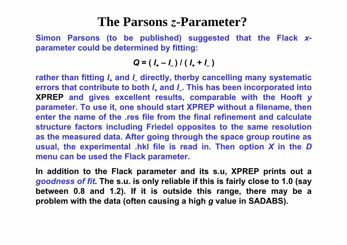
The Parsons z-Parameter?Simon Parsons (to be published) suggested that the Flack x-parameter could be determined by fitting:

Q = ( I+ – I– ) / ( I+ + I– )

rather than fitting I+ and I– directly, therby cancelling many systematic errors that contribute to both I+ and I–. This has been incorporated into XPREP and gives excellent results, comparable with the Hooft yparameter. To use it, one should start XPREP without a filename, then enter the name of the .res file from the final refinement and calculate structure factors including Friedel opposites to the same resolution as the measured data. After going through the space group routine as usual, the experimental .hkl file is read in. Then option X in the Dmenu can be used the Flack parameter.

In addition to the Flack parameter and its s.u, XPREP prints out a goodness of fit. The s.u. is only reliable if this is fairly close to 1.0 (say between 0.8 and 1.2). If it is outside this range, there may be a problem with the data (often causing a high g value in SADABS).

To merge or not to merge?The standard uncertainties (and comparison with known absolute configurations) indicate that, with good MoKa data (especially if measured to a higher resolution than usual), it is sometimes possible to determine the absolute structure with reasonable confidence even when the heaviest atom is oxygen.

Despite this, the experimental values of I+ and I– are strongly correlated, so the standard uncertainties of other parameters will be underestimated if Friedel opposites are not merged for the refinement (MERG 2). In such case MERG 4 is still strongly recommended (andavoids a CHECKCIF alert).

Scaling using equivalentreflections in SADABS and TWINABS I

D

Ic = Io ·S(n) ·P(u,v,w)S = Scale factor for frame n (incident beam I only)P = Absorption factor (diffracted beam D only)u,v,w = Direction cosines relative to a*, b* and c*

S and P are refined alternately to minimize Σw(<Ic> – Ic)2, where <Ic> is the mean of a group of equivalents. Scaling requires a high redundancy (MoO) to work well. SADABS and TWINABS use the same weighting scheme as CELL_NOW to downweight outliers, possibly temporarily; the mean weight is printed each cycle (if these values are less than about 0.8 probably something is seriously wrong).

Scaling is based on the followingapproximation:

SADABS and TWINABS strategyThese programs run in 3 stages that may be repeated if necessary:

1. Determine scaling and absorption parameters by fitting individual intensities to the mean corrected intensities (averaged over equivalents). Outliers are downweighted but not rejected in this stage. For parameter determination Friedel opposites should be treated as equivalent (i.e. Laue group symmetry imposed). For the remaining calculations it may be better to use the point group. For TWINABS, the ‘equivalents’ may be single reflections or groups of overlapping reflections that contribute to a single integrated intensity.

2. Delete a small number of reflections that are completely incompatible with their equivalents, e.g. reflections blocked by the beam stop etc. Then determine an error model for the remaining reflections by fitting 2 to unity to put (I) onto an absolute scale.

3. Output diagnostic statistics (graphically) and corrected data. TWINABS writes both HKLF 4 format files for structure solution and initial refinement and HKLF 5 files for final accurate refinement.

Incident beam scale factors

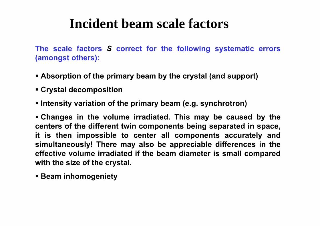
The scale factors S correct for the following systematic errors (amongst others):

Absorption of the primary beam by the crystal (and support)

Crystal decomposition

Intensity variation of the primary beam (e.g. synchrotron)

Changes in the volume irradiated. This may be caused by the centers of the different twin components being separated in space, it is then impossible to center all components accurately and simultaneously! There may also be appreciable differences in theeffective volume irradiated if the beam diameter is small compared with the size of the crystal.

Beam inhomogeniety

Diffracted beam absorption factorThe diffracted beam absorption factor P(u,v,w) is a sum of spherical harmonics for the direction cosines u, v and w as suggested by Blessing (1995). For example:

P0,1,2 = b1 + b2u + b3v + b4w +

b5(3w2-1)/2 + b6(3uw) + b7(3vw) + b8(3u2-3v2) + b9(6uv)

Since this is a linear function, only one refinement iteration is required. S and b are determined in alternate cycles; the incident beam scale factor depends linearly on S, so rapid convergence is assured and no initial values are needed for S and b.

Error modelAfter deleting severe outliers, the parameters k and g in the expression:

σ2(abs) = k [ σ2(raw) + g <I>2 ]

are adjusted so that χ2 is approximately unity for reflection batches based on mean intensity. σ(raw) is the e.s.d. of a particular intensity measurement in the .raw or .sad file from the integration and σ(abs) is output by SADABS.

A high value of g (>0.08) is a warning sign that there are problems with the data!

Needle-shaped crystal with axis along phi

SADABS diagnostics - shadows

SAINT attempts to make an active pixel mask so that reflections blocked by other objects are not integrated. In this example the active pixel mask was not generated correctly.

Strongly absorbing thick plate – spherical harmonics

Plus face indexed absorption correction in SADABS

Diffraction pattern of glucose isomerase triplet

MadhumatiSevvana

To index a multiple crystal, first a cell and orientation matrix are found to index as many reflections as possible, subject to the cell being as small as possible. This cell is then rotated (twice in this case) until most of the remaining reflections have been fitted too. SAINT then uses the orientation matrices (3 in this case) to integrate the data. Some reflections can be integrated independently, in other cases there are two or more overlapping reflectionscontributing to the same observed intensity. SAINT also attempts to make a rough partitioning of the intensities within an integration box, but this is much less accurate.

Non-merohedral protein twins

Cubic insulin twin Glucose isomerase triple crystal

Madhumati Sevvana

Note that whereas the two components of the cubic insulin twin are interpenetrant and so have approximately the same center, the three components of the GI ‘drilling’ have well separated centers.

Strategy for twinned crystals1. Find orientation matrices for all components, e.g. using

CELL_NOW.

2. Verify interpretation using RLATT.

3. Multicomponent integration using SAINT (or EVAL_CCD), write .mul (or .sam) file (multicomponent .raw file).

4. Process the data using TWINABS. This writes a standard HKLF 4 format .hkl file for structure solution and initial (isotropic) refinement plus a special HKLF 5 format file for the final refinement in which all reflections that contribute to the same ‘observation’ are grouped together. The reflections can be selected and merged in a variety of ways.

5. Structure solution and initial refinement in the usual way using the HKLF 4 format file.

6. Final refinement including twin fractions (BASF) using the HKLF 5 format file.

ThresholdingTo find reflections, first a smooth background must be established, so that it is possible to judge whether reflections are significantly greater than the background.

If a reflection is spread over several frames (common for fine slicing) its centroid in the rotation angle can be found, giving accurate 3D x, yand z coordinates. If it is only present on a single frame (common for wide frames) then the center of the rotation range has to be used, which is much less precise.

The reflection positions are very sensitive to the position of the ‘beam center’, i.e. the X and Y detector coordinates of the point at which the beam would hit the detector when the detector 2 angle is zero, so this position needs to be redetermined every time the detector is moved. If these parameters or the detector distance are significantly in error, straight reciprocal lattice lines will become curved etc. This can be seen before indexing by inspecting the thresholded reflection array with RLATT.

The reciprocal lattice

that constitute A so that the above equations are satisfied for all reflections with integer values for h, k and l. Then the reciprocal cell dimensions could be calculated, e.g.

(a*)2 = (ax*)2 + (ay*)2 + (az*)2; b*c*cos* = bx*cx* + by*cy* + bz*cz*.

but most indexing programs determine the REAL unit-cell!!

c*

b*

a*

001

002 012 022032

011 021 031

102 112 122 132

101 111 121 131

000 010 020030

100 110 120 130

x = Ah or

x = ax* h + bx* k + cx* l y = ay* h + by* k + cy* l z = az* h + bz* k + cz* l

ax*, ay* and az* are the components of a* in the orthogonal axis system. Indexing could involve finding the nine numbers

h, k, ℓ and the real cell?!What we actually want to do is to determine h,k,ℓ from x,y,z for each reflection, not vice versa, so we need to invert the matrixA: h = A–1x

which corresponds to: h = axx + ayy + azzk = bxx + byy + bzzℓ = cxx + cyy + czz

where ax, ay and az are the components of the real cell axis aalong the orthogonal axes, and a2 = ax

2 + ay2 + az

2 etc. So instead of having to find 9 parameters at once, we only need to find 3 – repeatedly – for the possible cell axes.

Each of these three equations can be considered to define a family of planes in reciprocal space. To find a unit-cell axis (we can decide later whether to call it a, b or c) we need to find three parameters dx, dy and dz so that t = dxx + dyy + dzz is close to integer for every reflection, i.e. the planes pass through all reflections. d is the perpendicular vector between the planes.

The cell_now algorithmThis is a brute-force algorithm and is intended only for use when all other methods fail. Multiple random real-space starting vectors d with lengths between user-input limits dmin and dmaxare refined by iterative linear least-squares refinement, using all reflections, minimizing the weighted sum of squares of the differences between t = dxx + dyy + dzz and m, the nearest integer to t for each reflection.

The trick is the weighting scheme w = I½p2 / (p2+(m-t)2), where p2 is the precision factor, usually 0.01, and I is the intensity. This strongly downweights reflections that do not fit well, i.e. [ (m–t)2 >> p2 ], and so concentrates the refinement on the better-fitting reflections, which in general will belong to the same twin domain.

Amazingly, this algorithm can index one component of a multicomponent twin, given enough CPU time.

Finding further twin componentsWith cell_now, the reflections that do not fit the first twin domain can be used to search for a second domain. Starting from a large number of random starting values of three rotation angles, the cell for the first domain is rotated to give a good fit to as many of these reflections as possible, using the same weighted least-squares criterion as for the first domain.

The rotation required (often 180° about a real or reciprocal axis) provides a description of the type of twinning.

After assigning reflections to the second domain, the reflections that do not fit either domain may be used to search for a third domain etc. in the same way. Cell_now can write the multidomain .spin or .p4p file needed for integration of such twins with SAINT.

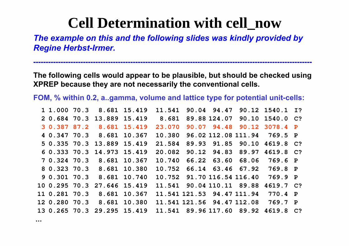
Cell Determination with cell_nowThe example on this and the following slides was kindly provided by Regine Herbst-Irmer.----------------------------------------------------------------------------------------------------------------

The following cells would appear to be plausible, but should be checked using XPREP because they are not necessarily the conventional cells.

FOM, % within 0.2, a..gamma, volume and lattice type for potential unit-cells:1 1.000 70.3 8.681 15.419 11.541 90.04 94.47 90.12 1540.1 I?2 0.684 70.3 13.889 15.419 8.681 89.88 124.07 90.10 1540.0 C?3 0.387 87.2 8.681 15.419 23.070 90.07 94.48 90.12 3078.4 P 4 0.347 70.3 8.681 10.367 10.380 96.02 112.08 111.94 769.5 P 5 0.335 70.3 13.889 15.419 21.584 89.93 91.85 90.10 4619.8 C?6 0.333 70.3 14.973 15.419 20.082 90.12 94.83 89.97 4619.8 C?7 0.324 70.3 8.681 10.367 10.740 66.22 63.60 68.06 769.6 P 8 0.323 70.3 8.681 10.380 10.752 66.14 63.46 67.92 769.8 P 9 0.301 70.3 8.681 10.740 10.752 91.70 116.54 116.40 769.9 P

10 0.295 70.3 27.646 15.419 11.541 90.04 110.11 89.88 4619.7 C?11 0.281 70.3 8.681 10.367 11.541 121.53 94.47 111.94 770.4 P 12 0.280 70.3 8.681 10.380 11.541 121.56 94.47 112.08 769.7 P 13 0.265 70.3 29.295 15.419 11.541 89.96 117.60 89.92 4619.8 C?

…

Cell_now (first domain)------------------------------------------------------------------------Cell for domain 1: 8.681 15.419 23.070 90.07 94.48 90.12

Figure of merit: 0.818 %(0.1): 87.0 %(0.2): 87.2 %(0.3): 89.4

Orientation matrix: 0.00632676 0.03399367 0.037055100.11366315 0.00778372 -0.00254995 -0.01982382 0.05467956 -0.02260331

Percentages of reflections in this domain not consistent with lattice types: A: 47.6, B: 49.9, C: 52.1, I: 52.1, F: 74.8, O: 68.4 and R: 66.8%

Percentages of reflections in this domain that do not have:h=2n: 50.4, k=2n: 51.5, l=2n: 13.3, h=3n: 67.0, k=3n: 69.8, l=3n: 70.4%

361 reflections within 0.200 of an integer index assigned to domain 1,361 of them exclusively; 53 reflections not yet assigned to a domain.------------------------------------------------------------------------

Cell_now (second domain)----------------------------------------------------------------------

Cell for domain 2: 8.681 15.419 23.070 90.07 94.48 90.12

Figure of merit: 0.941 %(0.1): 100.0 %(0.2): 100.0 %(0.3): 100.0

Orientation matrix: 0.00824846 0.04352904 0.03226658-0.11331218 -0.00585096 0.004248750.02108641 -0.04771791 0.02883242

Rotated from first domain by 180.0 degrees aboutreciprocal axis -0.001 0.502 1.000 and real axis 0.185 1.000 0.895

Twin law to convert hkl from first to -1.000 0.000 0.000this domain (SHELXL TWIN matrix): 0.136 -0.281 0.643

0.269 1.432 0.281

119 reflections within 0.20 of an integer index assigned to domain 2,53 of them exclusively; 0 reflections not yet assigned to a domain----------------------------------------------------------------------

Equivalent reflections and groupsh k l component (assuming point group mmm)1 -2 3 ….. 1

-1 -2 -3 ….. 1-1 -2 -3 ….. 2 ― not equivalent to the above singles-1 -2 -3 ….. -22 0 -4 ….. 11 2 -3 ….. -2

-2 0 -4 ….. 14 1 1 ….. -21 -2 -3 ….. -3 not equivalent to the other groups shown here

-1 1 2 ….. 1

equivalent singles

equivalent groups

In SHELX HKLF 5 format, a group of overlapping reflections is definedby negative component numbers for all but the last reflection in thegroup. For scaling purposes the component numbers MUST match.

Twinabs optionsIf the space group is known, TWINABS can eliminate systematic absences from composite reflections. This may require reorientatingthe cell (for all data), so this oprion is also now available.

Reflections for scaling are selected using a code number:

0: Each component is scaled separately using singles, the resulting scale factors are then also used to scale the composite reflections. This is almost always the best option, even when one component dominates, except when there are very few singles.

N: Derive a single set of scaling parameters using all singles and composites that contain component N, then apply to all singles and composites. This can be used when this component dominates and almost all reflections overlap.

–N: Derive a single set of scaling parameters using only singles and composites that contain at least one of the components 1…N, then apply to all singles and composities. Useful for a 4-component twin where components 1 and 2 dominate and many reflections overlap.

Scale factors and Rint for GI-triplet

In view of the large scale variations, option ‘0’ is essential for scaling. The smallest crystal (shown in red) was furthest from the center.

10 25 45 10 25 45 10 25 45 10 25 2

Scale factors and Rint for cubic insulin

For this interpenetrant twin, the two crystals have approximately the same center and so show little variation in scale.

0 0 35 35 0 0 35 35 0 0 35 35 2

The HKLF 4 format output fileIn previous versions of TWINABS this file was created using the SAINT partitioning of composite reflections and hoping that averaging over many equivalents would compensate for the approximations involved. Such an HKLF 4 file can still be created by asking SADABS to process one component in a .mul file (new in SADABS 2007-2).

The new TWINABS makes this file by ‘solving’ the almost linear set of equations in which the unknown parameters are the intensities of the unique reflections and the twin ratios, and the observations are the (total) intensities of the single and composite reflections. Since this system of equations may be ill-conditioned, the SAINT partitioning is applied in the form of weak restraints (extra observational equations). The algorithm is robust, converges fast and can process several million reflections in a few seconds. The twin ratios obtained are close to those from the HKLF 5 refinement.

There is an option to use only reflections containing particularcomponents for this analysis when one (or two) components dominate. It may be necessary to generate and test two or more HKLF 4 format files, but often the option ‘0’ (use all) is best.

Inconsistent component indexingThe new HKLF 4 algorithm has revealed a subtle and unexpected elefant trap. In the cases where the Laue symmetry is lower than the metric symmetry of the lattice, the component may be indexed inconcistently, even though CELL_NOW obtains the second and subsequent orientation matrices by rotating the first!

For the insulin twin, CELL_NOW had rotated the cell by about 180ºabout an axis parallel to a face diagonal of the cubic cell [1 1 0], leading to inconsistently indexed components. This is similar to the generation of a merohedral twin. The only warning sign was a high Rintfor the HKLF 4 deconvolution, the scaling is not affected by the inconsistent indexing!! A re-indexing option has been added that can also be used when the components have different hands (a form ofracemic twinning).

The HKLF 5 format output fileDespite the improvements in the ‘detwinned’ HKLF 4 format file, refinement tests show that refinement using HKLF 5 is still almost always slightly more precise. It is best to compare the R1 value after ‘merging for Fourier’ at the end of the HKLF 5 refinement so that approximately the same number of reflections are used.

TWINABS provides a comprehensive set of options for preparing this file and merging equivalent groups of overlapping reflections, and some trial and error will often be required. When one component dominates it is best to use only singles and composites involving it, and the option to delete certain singles to reduce ‘twin pairing errors’(a feature of SAINT) is often but not always better.

However the currently popular (especially amongst Acta Editors) argument that it is essential to use only an ‘independent’ set of reflections in the HKLF 5 refinement is a red herring. In such a case (e.g. when the option ‘0’ is used to select all reflections for HKLF 5) all that is necessary to get the correct parameter esds is to set the third L.S. parameter for SHELXL to the number of ‘observations’ in the HKLF file minus the number of reflections in the HKLF 4 file!

Small molecule testsGanges (P21) 2 components, one dominant: 23609 (1), 22709 (2) and 19846 (composite). Rint 4.70% (scaling) and 4.78% (HKLF 4). Twin ratio 94.6:5.4% (HKLF 4) and 95.5:4.5% (HKLF 5 refinement).

HKLF 4: (0/0) R1 3.49%, (0/1) 2.94%, (1/1) 2.81%

HKLF 5: (0/1) R1 2.80%, (0/1p): 2.97%, (1/1) 2.66%, (1/1p) 2.81%

Feoxet2 (P21/c) 4 components, 2 strong: 2902 (1), 3827(2), 4112(3), 4085 (4), 1298 (composite). Rint 1.67% (scaling) and 2.56% (HKLF 4). Twin ratio 67.2:30.8:1.1:0.9% (HKLF 4) and 67.6:30.4:1.7:0.3% (HKLF 5 refinement).

HKLF 4: (0/0) R1 2.24%, (0/-2) 2.52%. HKLF 5: (0/1) 2.09%, (0/1p) 2.02%.

JL55 (P21): 2 components, strong overlap. 1624 (1), 1793 (2) 19825 (composite). Rint 3.69% (scaling), 3.91% (HKLF 4). Twin ratio 83.5:16.5% (HKLF 4) and 86.0:14.0% (HKLF 5 refinement).

HKLF 4: (0/0) R1 6.81%, (1/0) 5.87%, (1/1) 4.66%.

HKLF 5: (0/1np) R1 3.91%, (1/1) 3.29%, (1/1p) 3.15%.

The incident angle problemThe efficiency f of the X-ray phosphor is the fraction of incident X-ray photons that it absorbs and reemits as visible light. More light photons are produced when the reflection comes in at a larger angle because the path length through the phosphor is longer. However if the phosphor is too thick it will reabsorb some of the light.

Phosphor (e.g. Gd2O2S)

X-ray reflection

Wu, Rodrigues & Coppens (J. Appl. Cryst, 35 (2002) 356-359) derived the correction required for the incident angle ; this was reformulated by Chambers, Kärcher & Ruf to give:

Icorrected = Iobs f / [1 – (1 – f)1/cos() ]This leads to corrections of up to 5% for MoK radiation, and the correction becomes larger for shorter (synchrotron) wavelengths. A ‘flood-field’ detector calibration is usually made for single wavelength systems but is rarely performed for different synchrotron wavelengths!

Calculating the angle of incidenceSADABS versions 2007/5 and later allow f to be refined during the parameter refinement. To calculate the angle for each reflection, the program first finds the coordinates xc, yc and zc of the crystal in the detector pixel coordinate system (each pixel is defined by its coordinates xp, yp on the detector; zp is always zero).

The position of the crystal relative to the detector is found by fitting the angles between reflections that strike the detector (almost) simultaneously. These angles are found (a) from the direction cosines of the reflections and (b) geometrically from the detector coordinates. This method is precise enough and very robust; no user input is required and the detector may be placed anywhere in any orientation!

xc,yc,zc

xp1,yp1,0 xp2,yp2,0

It is then trivial to calculate cos() for each reflection from its detector coordinates and those of the crystal.

Test results1. SMART6000 with CuK radiation: f refines very close to 1.0, no effect on the remaining parameters. Clearly the interpolation of the flood-field correction for different distances is working and anyway the correction is small for CuK.

2. Various APEX-II detectors with MoK: 0.76 < f < 0.87. Rintdecreases by about 0.001 and the g value for the weighting scheme decreases significantly; however there is very little change in the R1 and wR2 (or even the Uij) values for the IAM refinement!

For shorter wavelengths (AgKa or synchrotron data) the angle of incidence effects are expected to be larger.

Conclusions and AcknowledgementsThe improvement in the HKLF 4 treatment means that a full HKLF 5refinement – with testing of the different options for preparing the HKLF 5 file – only needs to be performed right at the end of the refinement (if at all).

Collecting data from non-merohedrally twinned crystals leads to an increase in the number of reflections that can be collected in a given time and to improvements in the redundancy and completeness of the data – minor components do not suffer from overloads – and so should become normal practice, both for small and macromolecules!

I am very grateful to my group in Göttingen and many CELL_NOW, SADABS and TWINABS users for their help in optimizing the program, in particular to Regine Herbst-Irmer, Madhumati Sevvana, Victor Young, Peter Jones and Ina Dix.