recent advances on force identification in structural...

Chapter 6

Recent Advances on ForceIdentification in Structural Dynamics

N. M. M. Maia, Y. E. Lage and M. M. Neves

Additional information is available at the end of the chapter

http://dx.doi.org/10.5772/51650

1. Introduction

This chapter presents recent advances on force identification for structural dynamics that havebeen developed by the authors using the concept of transmissibility for multiple degree-of-freedom (MDOF) systems.

Being applied for many years only to the single degree-of-freedom (SDOF) system or to MDOFsystems in a very limited way, the transmissibility concept has been developed along the lastdecade or so in a consistent manner, to be applicable in a general and complete way to MDOFsystems. Various applications for MDOF systems may now be found, such as evaluation ofunmeasured frequency response functions (FRFs), force identification, detection of damage,etc. A review of the multiple applications of the transmissibility concept has been publishedrecently [1].

It is the application of this generalized transmissibility concept to both the direct and inverseforce identification that is described along this chapter. The direct problem is understood asthe one where one knows the applied forces and wishes to estimate the reactions at thesupports; the inverse force identification problem is when one wishes to determine how manyforces are applied, where they are applied and which are their magnitudes.

To determine the location and magnitude of the dynamic forces that excite the system isan important issue in structural dynamics [2, 3], especially when operational forces cannotbe directly measured, as it happens at inaccessible locations [4, 5]; it is often the case thattransducers cannot be introduced in the structure to allow the experimental measurementof the external loads and only a limited number of sensors and positions are available.The identification of forces from vibration measurements at a few accessible locations is a

© 2012 Maia et al.; licensee InTech. This is an open access article distributed under the terms of the CreativeCommons Attribution License (http://creativecommons.org/licenses/by/3.0), which permits unrestricted use,distribution, and reproduction in any medium, provided the original work is properly cited.

very important problem in various areas, such as vibration control, fatigue life predictionand health monitoring.

Although the force identification problem may be solved from the dynamic responses bysimply reversing the direct problem, this is usually ill-posed and sensitive to perturbations inthe measured data.

Over the past years, the theory of inverse methods has been actively developed in manyresearch areas presenting in common the effects of matrix ill-conditioning, reflecting the ill-posedness nature of the inverse problem itself. Those problems can often be overcome bymethods such as pseudo-inversion for over-determined systems, use of Kalman filters [6, 7],Singular Value Decomposition and Tikhonov regularization [8-10].

Various research works in force identification can be found in the literature, such as thoserelated to the identification of impact forces, implementation of prediction models based onreflected waves or simply from the dynamic responses [11-18], prediction of forces in platesfor systems with time dependent properties [11] and identification of harmonic forces [13].

These methods to identify operational loads based on response measurements can be clas‐sified into three main categories: deterministic methods, stochastic methods and methodsbased on artificial intelligence. Two main classes of identification technique are consid‐ered in the group of deterministic methods for load identification: frequency-domainmethods and time-domain methods. The force identification in time domain has been lessstudied than its frequency domain equivalent, therefore there are not that many forceidentification studies in the literature. A review on the state of the art for dynamic loadidentification may be found in [3, 14].

Although out of the scope of this chapter, some references are here given with respect to recenttime-domain force identification developments. One interesting approach based on modalfiltering [15] is the Sum of Weighted Accelerations Technique (SWAT), which allows to obtainthe time-domain force reconstruction by isolating the rigid body modal accelerations. Anotherapproach for time-domain force reconstruction is the Inverse Structural Filter (ISF) method ofKammer and Steltzner [16] that inverts the discrete-time equations of motion. A variant of this,expected to produce a stable ISF when the standard method fails was recently developed andnamed as Delayed Multi-step ISF (DMISF). For a more detailed description on these methods(SWAT, ISF and DMISF) see e.g. [17] and for its application to rotordynamics, see [18].

In this chapter, the authors treat the frequency-domain problem from a different perspective,which is based on the MDOF transmissibility concept. As aforementioned, usually thetransmissibility of forces is defined in textbooks for SDOF systems, simply as the ratio betweenthe modulus of the transmitted force magnitude to the support and the modulus of the appliedforce magnitude. For SDOF systems, the expression of either the transmissibility of motion orforces is exactly the same; however, as explained in [1], that is not the case for MDOF systems.On the one hand, the problem of extending the idea of transmissibility of motion to an MDOFsystem is essentially a problem of how to relate a set of unknown responses to a set of knownresponses associated to a given set of applied forces; on the other hand, for the transmissibilityof forces the question is how to relate a set of reaction forces to a set of applied ones.

Advances in Vibration Engineering and Structural Dynamics104

Some initial attempts on the generalization of the transmissibility concept are due toVakakiset al. [19-21], Liu et al. [22, 23] and Varoto [24]. Similar efforts can also be found in the indirectmeasurement of vibration excitation forces [2, 4, 5]. To the best knowledge of the authors, ageneral answer to the problem is due to Ribeiro [25], and in [26] the experimental evaluationof the transmissibility concept for MDOF systems is presented. The concept of transmissibilityof forces for MDOF has been proposed in 2006 [27], where the authors explain the formulationof the transmissibility using both the dynamic stiffness and the receptance matrices.

The use of the transmissibility in conjunction with a two step methodology for force identifi‐cation is the main novelty of this chapter. For the force identification based on the transmissi‐bility of motion, two steps are taken, (i) firstly the number of forces and their location areobtained, and (ii) secondly the reconstruction of the load vector is performed using some ofthe responses obtained experimentally together with the updated numerical model. Both havebeen numerically developed and implemented, as well as experimentally tested in the researchgroup during the last years to access the potential of these new methods.

In section 2, the authors review the generalized transmissibility concepts, both in terms ofdisplacements and forces. They are introduced and deduced from two different perspectives,(i) from the frequency response functions, (ii) from the dynamic stiffness.

In section 3, a numerical model and an experimental application are presented to illustratedthe transmissibility concept.

In section 4 the methodologies proposed for force identification based on the transmissibilityconcept are introduced.

Some simulated and experimental results are presented to show how these methodologies areable to help us identifying applied and reaction forces. The authors present a discussion onthese proposed methods and on the obtained results.

2. Transmissibility in MDOF systems

The transmissibility concept may be found in any fundamental textbook on mechanicalvibrations (e.g. [28]), related to SDOF systems.

The transmissibility of motion is defined as the ratio between the modulus of the responseamplitude (output) and the modulus of the imposed base harmonic displacement (input).Depending on the imposed frequency, the result can vary from an amplification to an attenu‐ation in the response amplitude relatively to the input one.

On the other hand, the transmissibility of force is defined as the ratio between the modulus ofthe transmitted force magnitude to the support and the modulus of the imposed forcemagnitude.

It happens that for SDOF systems the expression for calculating the transmissibility is the same,either referring to forces or to motion. This is not the case for MDOF systems.

Recent Advances on Force Identification in Structural Dynamicshttp://dx.doi.org/10.5772/51650

105

The generalization of these definitions to MDOFs has been developed in the last decade, asmentioned before. In this section a brief review of these generalizations is given, introducingalso the concepts and notation used for the force identification problem.

2.1. Transmissibility of motion in MDOF systems

To introduce the problem, the authors follow here as near as possible the notation used in [1].Let K be the set of nK co-ordinates where the displacement responses YK are known (measuredor computed), U the set of nU co-ordinates where the displacement responses YU are unknown,and A the set of co-ordinates where the forces FA may be applied (Fig. 1).

Figure 1. Illustration of an elastic body with the three sets of co-ordinates K, U and A.

To obtain the needed transmissibility of motion one may consider two distinct ways. The firstis based on the frequency response function (FRF) matrices H(ω), known as the fundamentalformulation, while the second is based on the dynamic stiffness matrix Z(ω) and is namedalternative formulation.

The receptance frequency response matrix H(ω) relates the dynamic displacement amplitudesY with the external force amplitudes F as (using harmonic excitation, in steady-state condi‐tions):

( ) 12 w w-

= Û = - + iY H F Y K M C F (1)

where K, M and Care the stiffness, mass and viscous damping matrices, respectively. H(ω)includes all the degrees of freedom in which the system is discretized and corresponds to the


inverse of the dynamic stiffness matrix Z(ω). One may underline that the mass-normalizedorthogonality properties are observed here:

2( )w

=

=

Φ Φ IΦ Φ diag

T

Tr

MK

(2)

Assuming proportional damping, C=αK+βM and therefore,

Y = H F = Φ diag(ωr2−ω 2) + i ω(α diag(ωr

2) + β I ) −1 Φ T F (3)

where Φ is the mode shape matrix, ωr is the rth natural frequency and α and β are constants.

From (1) it is easy to understand that if the responses Y at the discretization points are known,then the force reconstruction (in frequency-domain) would be given by:

1-=F H Y (4)

2.1.1. Transmissibility of motion in terms of FRFs

Based on harmonically applied forces at co-ordinates A, one may establish that displacementsat co-ordinates U and K are related to the applied forces at co-ordinates A by the followingrelationships:

=U UA AY H F (5)

=K KA AY H F (6)

Eliminating the external forces FA between (5) and (6), one obtains

( ) ( )+

= = AU UA KA K d KUKY H H Y T Y (7)

where

( ) ( )+=Ad UA KAUKT H H (8)

is the transmissibility matrix relating both sets of displacements. (HKA)+ is the pseudo-inverseof the sub-matrix HKA. An important property of the transmissibility matrix to be used here isthat it does not depend on the magnitude of the involved forces and only requires the


107

knowledge of a set of co-ordinates that include all the co-ordinates where the forces are applied.Indeed, it is required that nK be greater or equal to nA. One important aspect of this definitionis that sub-matrices HUA and HKA may be obtained experimentally.

2.1.2. Transmissibility of motion in terms of dynamic stiffness

There exists an alternative approach to obtain the transmissibility matrix for the displacements,using the dynamic stiffness matrices introduced in (1). Assuming again harmonic loading anddefining two subsets, A and B, A being the set where the dynamic loads may be applied andB the set formed by the remaining co-ordinates, where no forces are applied (FB = 0), one canobtain (after grouping adequately the degrees of freedom of the problem):

é ù ì ü ì ü=í ý í ýê úî þî þë û 0

K AAK AU

UBK BU

Y FZ ZYZ Z

(9)

Developing eq. (9), it follows that

a

b

+ =

+ = 0AK K AU U A

BK K BU U

YZ Z Y FZ Y Z Y

(10)

From (10b) one obtains the transmissibility in terms of the dynamic stiffnesses:

( ) ( )+

= - = AU BU BK K d KUKY Z Z Y T Y (11)

where (ZBU)+ is the pseudo-inverse of ZBU.

From (11) it is possible to obtain the response at the unknown co-ordinates, as long as thepseudo-inverse is viable, which requires that nB is greater or equal to nU.

Indeed, from all this resulted two conditions:

( ) ( ) ( ) and + +

= - ³ ³Ad BU BK UA KA B U K AUK n n n nT Z Z = H H (12)

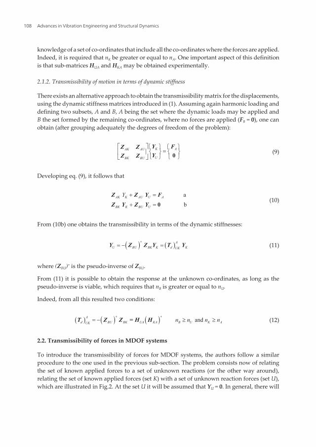
2.2. Transmissibility of forces in MDOF systems

To introduce the transmissibility of forces for MDOF systems, the authors follow a similarprocedure to the one used in the previous sub-section. The problem consists now of relatingthe set of known applied forces to a set of unknown reactions (or the other way around),relating the set of known applied forces (set K) with a set of unknown reaction forces (set U),which are illustrated in Fig.2. At the set U it will be assumed that YU = 0. In general, there will


be other co-ordinates, where neither there are any applied forces nor there are any reactions,that shall constitute the set C.

Figure 2. Illustration of both sets of co-ordinates K and U.

2.2.1. Transmissibility of forces in terms of FRFs

With the definition of the new sets K, U and C, the problem may be defined in the followingway:

é ùì üì üê úï ï =í ý í ýê úî þï ï ê úî þ ë û

K KK KUK

U UK UUU

C CK CU

Y H HF

Y H HF

Y H H(13)

Imposing YU = 0, it follows that

+ =UK K UU UH F H F 0 (14)

and so

( ) =U f KUKF T F (15)


109

where

( ) ( ) 1-= -f UU UKUK

T H H (16)

is the force transmissibility matrix.

This is the direct force identification method, i.e., one knows the applied forces and calculatethe reactions at the supports, where the displacements are assumed as zero. The inverseproblem is also possible, if one is able to measure the reaction forces and if their number ishigher than the number of applied forces, in order to calculate the pseudo-inverse of HUK:

( )( ) +

=K f UUKF T F (17)

where

( )( ) ( )+ += -f UK UUUK

T H H (18)

Note that in spite of the fact that here the reaction forces are known, the notation U (that inprinciple stands for “unknown”) is kept.

In the inverse problem, one may not know how many applied force exist and where they areapplied. If that is the case, one must follow a different approach, as it will be explained insection 4.1

If the condition YU = 0 is relaxed, from eq. (13) it follows that:

= +U UK K UU UY H F H F (19)

( ) ( )

( )( ) ( )

1a

and

b

-

+ +

= +

= +

U f K UU UUK

K f U UK UUK

F T F H Y

F T F H Y

(20)

2.2.2. Transmissibility of forces in terms of dynamic stiffness

Again, there is an alternative approach to obtain the force transmissibility matrix, using thedynamic stiffness matrices.


Assuming harmonic loading and the mentioned sets K, U and C, one can obtain (after groupingadequately the degrees of freedom of the problem) the following result:

é ù ì ü ì üê ú ï ï ï ï=í ý í ýê ú

ï ï ï ïê ú î þ î þë û

KK KC KU K K

CK CC CU C C

UK UC UU U U

Z Z Z Y FZ Z Z Y FZ Z Z Y F

(21)

It is worthwhile noting that joining together the sets K and C in a new set E makes it easier tosee that imposing YU = 0 one obtains the following relationships:

é ù ì üì ü=í ý í ýê ú

î þ î þë û 0EEEE EU

UUE UU

FYZ ZFZ Z

(22)

from which it is clear that:

a

b

=

=EE E E

UE E U

Z Y FZ Y F

(23)

Eliminating YE between (23a) and (23b), it turns out that

( )=U f EUEF T F (24)

where

( ) ( ) 1-=f UE EEUE

T Z Z (25)

The inverse problem corresponds to

( )( )+=E f UUEF T F (26)

with

( )( ) ( )+ +=f EE UEUE

T Z Z (27)


111

It is important to note that only some of the co-ordinates of the set E have applied forces. Thismeans that in (23) some rows of FE are zero and only the columns (in ZEE) whose co-ordinateshave applied forces (set K) are needed for the transmissibility matrix. In other words, from theset E only the co-ordinates corresponding to the K set are used.

2.3. Summary

From sections 2.2.1 and 2.2.2, one can conclude that for the direct problem of transmissibilityof forces there is no restrictions in the number of co-ordinates used:

( ) ( )( ) ( )

1

1

-

-

= -

=

f UU UKUK

f UE EEUE

T H H

T Z Z(28)

whereas in the inverse problem of transmissibility of forces there are some restrictions that canmake this option not very useful in practice, especially when using the dynamic stiffnesses,since one needs to calculate the pseudo-inverse matrices:

( )( ) ( )

( )( ) ( )

+ +

+ +

= - ³

= ³

f UK UU U KUK

f EE UE U EUE

n n

n n

T H H

T Z Z(29)

3. Numerical and experimental applications

As explained before, the transmissibility matrices may be obtained from a numerical model(which should be updated for the range of frequencies involved) or from results obtainedexperimentally. In this section, the methodology used in each case is described and illustratedthrough a comparison example.

3.1. Transmissibility in terms of the numerical model

For the numerical model, one needs the knowledge of the structure within the discretizationchosen, to create the receptance matrix H(ω), which is the inverse of the correspondingdynamic stiffness matrix Z(ω). Here, the numerical model is created using the Finite ElementMethod (FEM), although other alternatives may also be used. As seen before, the dynamicstiffness matrix is defined as:

2( ) w w w= - + iZ K M C (30)


where C represents the viscous damping matrix, often of the proportional type, i.e., C=αK+βM,where α and β are constants to be evaluated experimentally.

To build the dynamic stiffness matrix, a specific structural finite element is chosen accordingto the approximation considered. For example, in the case of a reasonably long and slenderbeam one can use the Euler-Bernoulli beam element (instead of a shell or solid structuralelement). Then, the global matrices are assembled for the chosen discretization of the structure.

In order to improve the accuracy of the numerical model when simulating what is obtainedexperimentally, concentrated masses are often added at the corresponding nodes to model theeffect of the accelerometers used in the testing positions.

Although the receptance matrix H(ω) is the inverse of the corresponding dynamic stiffnessmatrix, one should avoid such direct numerical inversion (frequency by frequency). Instead,H(ω) is calculated from eq. (3), after a modal analysis in free vibration.

Then, using (8) or (16), one can calculate the needed transmissibility matrices (Td)UKA or (Tƒ)UK.

Of course, alternatively one may use the equivalent expressions (11) or (25), respectively.

3.2. Transmissibility in terms of experimental measurements

Depending on the type of transmissibility to obtain, the corresponding experimental setupshould be established. Essentially, it is important to observe that for the transmissibility ofmotion one measures the FRFs relating co-ordinates U and K with co-ordinates A, normallyusing accelerometers and force transducers. For validation purposes, one may also measurethe applied forces. In the examples presented next for the transmissibility of motion, asuspended (free-free) beam is always used.

For the transmissibility of forces, in the direct problem, one measures the applied forces at co-ordinates K (in the inverse problem, one measures the reaction forces at co-ordinates U). Forvalidation purposes, one also measures the ones to be estimated. The test specimen for thetransmissibility of forces is always a simply supported beam.

For the experimental setup, the following equipment is used:

• Vibration exciter (Brüel & Kjær Type 4809);

• Power amplifier (Brüel & Kjær Type 2706);

• Force transducers(PCB PIEZOTRONICS Model 208C01);

• Data acquisition equipment (Brüel & Kjær Type 3560-C).

In Fig. 3, a schematic representation of the experimental setup used for the force transmissi‐bility tests is presented, in this case a simply supported beam with a single applied force.

The excitation signal used was a multi-sine transmitted to the exciter, with constant amplitudein the frequency. In reality the signal measured by the force transducer does not exhibits aconstant amplitude along the frequency, as it depends on the dynamic response of thestructure.


113

Figure 3. Example of the experimental setup developed for the transmissibility of forces.

For the transmissibility of motion, a beam suspended by nylon strings is used, to simulate free-free conditions. In order to facilitate the interchange of the available accelerometers betweenthe measure positions without affecting the dynamics of the structure, it is important to addequivalent masses (dummies) to model the effect of the sensors.

After obtaining experimentally the needed receptances, by using (8) or (16) one can establishthe transmissibility matrices (Td)UK

A or (Tƒ)UK.

3.3. Examples

The same steel beam was used in all the examples. With the purpose of illustrating theapplicability of the presented formulations to obtain the transmissibility plots, the authors usedthe geometric and material parameters presented in Table 1. Note that these data correspondto the values obtained after updating the FE model.

Young’s modulus – E 208 GPa

Density – ρ 7840 kg/m3

Length – L 0.8 m

Section width - b 5.0 × 10−3m

Section height - h 20.0 × 10−3m

Section area - A 1 × 10−4m 2

Second moment of area - I 2.0883 × 10−10m 4

proportional damping - α 4 s

proportional damping - β 2.0 × 10−6s −1

Table 1. Beam properties (after updating).


3.3.1. Numerical model

The standard two-node Euler-Bernouli bidimensional finite element is used here to build theneeded numerical model of the beam.

The beam was discretized into sixteen finite elements, which correspond to N = 17 nodes,ordered from 1 up to 17. As the analysis and the model are limited to the plane xOy, each nodehas three degrees of freedom (which are ux, uy, θ). Hence, the matrices of the numerical modelhave an order of 3xN for the free-free beam. In what the measurements are concerned, onlythe displacements and applied forces along the y direction are used and therefore the num‐bering of nodes and co-ordinates y coincide.

The model was updated using E, ρ and I as updating parameters and a proportional dampingmodel is included using α and β as updating parameters (Table 1).

3.3.2. Example 1 — Transmissibility of motion

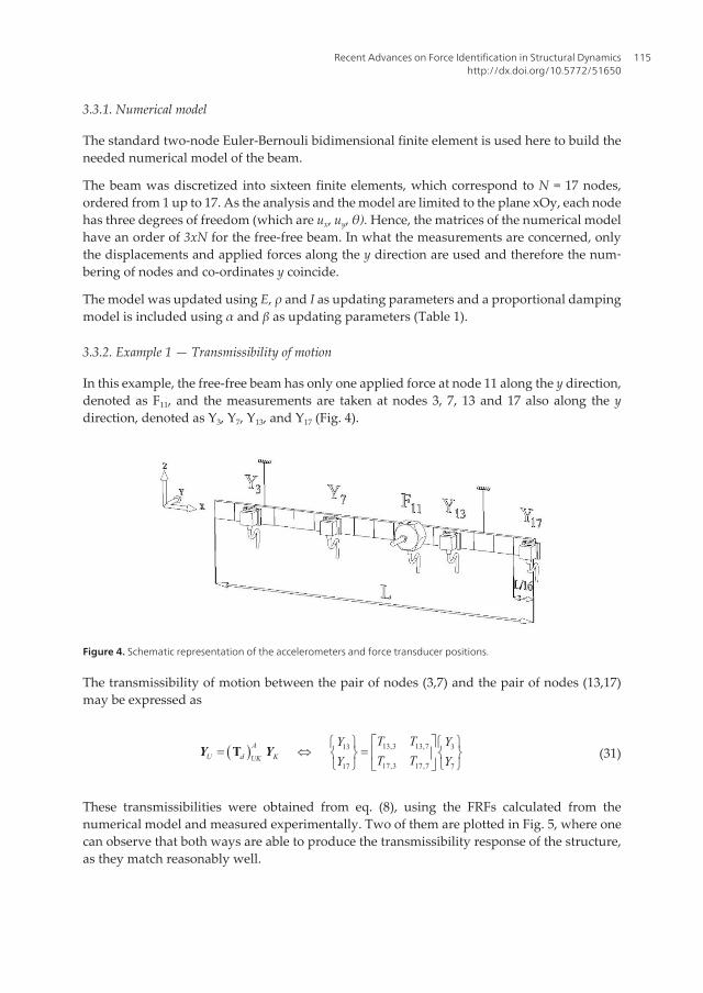
In this example, the free-free beam has only one applied force at node 11 along the y direction,denoted as F11, and the measurements are taken at nodes 3, 7, 13 and 17 also along the ydirection, denoted as Y3, Y7, Y13, and Y17 (Fig. 4).

Figure 4. Schematic representation of the accelerometers and force transducer positions.

The transmissibility of motion between the pair of nodes (3,7) and the pair of nodes (13,17)may be expressed as

( ) 13,3 13,713 3

17,3 17,717 7

é ùì ü ì ü

= Û =í ý í ýê úî þ î þë û

T AU d KUK

T TY YT TY Y

Y Y (31)

These transmissibilities were obtained from eq. (8), using the FRFs calculated from thenumerical model and measured experimentally. Two of them are plotted in Fig. 5, where onecan observe that both ways are able to produce the transmissibility response of the structure,as they match reasonably well.


115

Figure 4. Schematic representation of the accelerometers and force transducer positions.

The transmissibility of motion between the pair of nodes (3,7) and the pair of nodes (13,17) may be expressed as

13,3 13,713 3

17,3 17,717 7

A

U d KUK

T TY Y

T TY Y

TY Y

(31)

These transmissibilities were obtained from eq. (8), using the FRFs calculated from the numerical model and measured

experimentally. Two of them are plotted in Fig. 5, where one can observe that both ways are able to produce the transmissibility

response of the structure, as they match reasonably well.

Figure 5. Numerical and experimental transmissibilities (upper plot, T13,3; bottom plot, T13,7)

0 50 100 150 200 250 300-80

-60

-40

-20

0

20

Frequency (Hz)

Am

plit

ude

(dB

)

Numerical motion trasmissibilityExperimental motion trasmissibility

0 50 100 150 200 250 300-80

-60

-40

-20

0

20

Frequency (Hz)

Am

plit

ude

(dB

)

Numerical motion trasmissibilityExperimental motion trasmissibility


Figure 6. Schematic representation of the positions of the force transducers.


3.3.3. Example 2 — Transmissibility of forces

In this case, a simply supported beam is considered with one applied force at node 7 andreactions at nodes 1 and 17. Only the magnitude of the forces is measured, and the transmis‐sibility is obtained directly from the measurements and compared with the numerical results.The experimental setup is illustrated in Fig. 6.

The force transmissibility relation between node 7 and the pair of nodes (1,17) may beexpressed as

{ }1,717

17,717

é ùì ü=í ý ê ú

î þ ë û

TFF

TF (32)

Figure 6. Schematic representation of the positions of the force transducers.

3.3.3. Example 2 — Transmissibility of forces

In this case, a simply supported beam is considered with one applied force at node 7 and reactions at nodes 1 and 17. Only the

magnitude of the forces is measured, and the transmissibility is obtained directly from the measurements and compared with the

numerical results. The experimental setup is illustrated in Fig. 6.

The force transmissibility relation between node 7 and the pair of nodes (1,17) may be expressed as

1,717

17,717

TFF

TF

(32)

The force transmissibilities were obtained using eq. (16) and are plotted in Fig. 7, where it is clear that both numerical and

experimental FRFs are able to produce the transmissibility response of the structure. Note that around 100 Hz there is a “bump” in

the experimental curve, due to the effect of the supports of the beam themselves; this effect has not been included in the numerical

model because it was not important, as these results are only of an illustrative type.


4. Force identification

0 50 100 150 200 250 300-50

-40

-30

-20

-10

0

10

20

30

Frequency (Hz)

Am

plit

ude

(dB

)

Numerical force transmissibilityExperimental force transmissibility

0 50 100 150 200 250 300-50

-40

-30

-20

-10

0

10

20

30

Frequency (Hz)

Am

plit

ude

(dB

)

Numerical force transmissibilityExperimental force transmissibility



117

The force transmissibilities were obtained using eq. (16) and are plotted in Fig. 7, where it isclear that both numerical and experimental FRFs are able to produce the transmissibilityresponse of the structure. Note that around 100 Hz there is a “bump” in the experimental curve,due to the effect of the supports of the beam themselves; this effect has not been included inthe numerical model because it was not important, as these results are only of an illustrativetype.

4. Force identification

This section shall be divided into (i) part one for the force localization algorithm based on thetransmissibility of motion and reconstruction using the measured responses and the updatednumerical model, and (ii) part two for the force reconstruction using the transmissibility offorces.

4.1. Force localization based on the transmissibility of motion and force reconstruction

The force identification problem is a difficult matter, as one has a limited knowledge of themeasured responses, due to the complexity of the structure, lack of access to some locations,etc. In other words, there are difficulties due to the incompleteness of the model.

Due to this difficulty in calculating the load vector directly, the authors propose to divide theprocess into two distinct steps:

1. the localization of the forces, i.e. the identification of the number and position of theapplied forces using the concept of transmissibility of motion;

2. the load vector reconstruction.

For the first step, a search for the number and position of forces using the transmissibility ofmotion is performed. Essentially, this step consists of searching for the transmissibility matrixcorrespondent to the dynamics of the system and using the available measured data and thenumerical model involved.

Once the corresponding transmissibility matrix is found, one has a solution for the numberand position of the forces applied to the structure.

The second step consists of reconstructing the load vector with the results obtained in the firststep. A more detailed description about this methodology is given in the following sections.

4.1.1. Force localization

In a first stage, to apply the method proposed in the previous section, one finds the transmis‐sibility matrix that converts the dynamic responses YK into YU. As one does not know theposition of the applied forces, it was decided to cover all the possibilities until the calculatedresponses (YU) match the measured ones Ỹ, over a range of frequencies. To calculate the vectorYU one may use either eq. (7) or (11).


The maximum number of forces must be less or equal to the dimension of the known dynamicresponse vector Y.

The successive combinations of the tested nodes are obtained according to the followingscheme:

The error in each combination is kept in a vector to identify the combination with the leastassociated error (in absolute value). Firstly, the algorithm scrolls through the possible combi‐nations of position and number of forces. For each combination, the associated error betweenthe calculated vector YU and the measured response vector Ỹ is calculated; this is carried outover a frequency range defined by the user. The error between the predicted and the measureddynamic response at each co-ordinate i can be defined as:

( )( ) ( )( )( )2error log abs ( ) log abs ( )

w

w w= -å %i ii U UY Y (33)

For each combination, the calculated error is kept in an entry of the error vector and analyzedlater on:

{ }ierror=ε (34)

The accumulated error for a given combination of co-ordinates where F can be located is thenorm of ε. The calculations are repeated for sucessive combinations of number and positionof forces. The combination of the force locations that gives the lowest error leads to the numberand position of the forces applied to the structure. As already mentioned, the maximumnumber of forces that can be found is equal to the dimension of the known dynamic responsevector.

As one does not know a priori how many forces exist, one has to follow a trial and errorprocedure that consists basically in assuming an increasing number of forces and the corre‐sponding number of measurements; if the right number of forces is Nf, one has a minimum


119

error ε for a certain set of co-ordinates. When one proceeds and assumes Nf +1 forces andmeasurements, the error will be higher then ε, telling us that the right answer was effectivelyNf at a certain set of co-ordinates.

It is clear that all the combinations of the Nf +1 forces that contain the right combination of theNf forces should exhibit a local minimum, though not the absolute one.

The method was implemented computationally (in MatLab®).

4.1.2. Force reconstruction

In a second step, the reconstruction of the force amplitudes consists of solving an inverseproblem using the measured dynamic responses YK:

( )+=A KA KF H Y (35)

Note that for the given system to be invertible, the number of dynamic responses to be used(set K) must be higher or equal than the number of applied forces (set A). However, this isalways verified, as in the first step one has already imposed it.

4.1.3. Example 3 — Localization of the applied forces

This is a numerical example, illustrated in Fig.8, where a set of uncorrelated forces is appliedat co-ordinates 1 and 5 (set A), and one uses the three known responses (set K) to identify thenumber and location of forces.

A set of simulated results (to mimic the experimental measurements) are obtained at nodes 1,3, 5, 11 and 17 (see Fig. 8); they define the following sets:

{ } { }3 5 17 1 11 and = =Y YT TK UY Y Y Y Y (36)

Figure 8. Illustration with the responses and applied force locations for example 3.


Considering these responses, the maximum number of identifiable applied forces is three, asexplained before. The forces are uncorrelated and applied to the structure at co-ordinates 1and 5. A series of force combinations have to be systematically generated as follows. In thiscase, all combinations up to three forces have been considered:

Applying the localization method described in the previous subsection 4.1.1, one obtains theplot of the error defined in eq. (33), as shown in Fig.9.

0 100 200 300 400 500 600 700 80010-30

10-20

10-10

100

1010

combination number

accu

mul

ated

err

or

Figure 9. Accumulated error in frequency for each combination of forces.

It is clear that there are several situations (combinations) where the error is close to zero andother where is not.

The minimum error happens with the combination number 21, corresponding to two forcesapplied at co-ordinates 1 and 5, thus identifying the correct positions and number of forces(Table 2).


121

Combination Number of forces Position of the forcesNumber of

identified forces

Identified

positions

Absolute

error

21 2 1, 5 2 1, 5 2,69e-29

Table 2. Data of the combination with minimum error.

To better understand why there exist more combinations with small errors, Table 3 shows thesecombinations with its corresponding error value. All of them have a common group of co-ordinates, corresponding to the correct combination of number and positions of the forces. Inthis case the correct positions are obtained with success through the minimum error.

Combination Real position of the forces Absolute error

21 1,5 2,69e-29

156 1,2,5 7,99e-26

170 1,3,5 2,85e-27

183 1,4,5 6,99e-28

197 1,5,7 8,70e-29

198 1,5,8 1,86e-28

199 1,5,9 1,82e-28

200 1,5,10 5,54e-28

Table 3. Some combinations and their respective error.

This illustrates the localization step performed with two forces, whose number and locationwere not known at the beginning. From these results, it can be stated that the transmissibilityof motion can be considered as adequate to perform this task. Note that, in spite of the highnumbers of combinations that exist, the computations are relatively quick, as they involve onlysub-matrices, and for the first permutations they are of a small order.

4.1.4. Example 4 — Localization and reconstruction 1

This is an experimental example, where a multisine signal is fed into the shaker, attached tothe beam at co-ordinate 13. Later on, the applied force is compared with the reconstructed one.

The experimental measurements are obtained at nodes 5, 7, 11 and 15. The measured vectorsare as follows:

{ } { }7 15 5 11 and = =Y YT TK UY Y Y Y (37)


Considering these responses, the maximum number of identifiable applied forces is two, asexplained before.

A series of force combinations was systematically generated as described before. Applying thelocalization method, one obtains the graph of Fig. 10.

4.1.4 Example 4 – localization and reconstruction 1

This is an experimental example, where a multisine signal is fed into the shaker, attached to the beam at co-ordinate 13. Later on, the applied force is compared with the reconstructed one.

The experimental measurements are obtained at nodes 5, 7, 11 and 15. The measured vectors are as follows:

7 15 5 11 and T T

K UY Y Y Y Y Y (37)

Considering these responses, the maximum number of identifiable applied forces is two, as explained before.

A series of force combinations was systematically generated as described before. Applying the localization method, one obtains the graph of Fig. 10.

Figure 10. Accumulated error in frequency for each force combination.

As one can see, the absolute minimum corresponds to combination no. 13, which is right because this combination represents the force applied at co-ordinate 13. So, the method could localize correctly the position of the force at co-ordinate 13.

Once the localization of the force is accomplished, its reconstruction is a simple calculation, using the measured displacements relating those co-ordinates to the force location. As the force is located at node 13, taking the measurement at co-ordinates 5, 7, 11 and 15, for instance, it follows that:

5 55,13 5,13

7,13 7,137 713 13

11,13 11,1311 11

15,13 15,1315 15

Y YH H

H HY YF F

H HY YH HY Y

(38)

Using the information from the measured responses, the reconstruction is now immediate. To validate this methodology, the result was ploted against its experimentally measured curve, as in Fig. 11. One may affirm that the method is able to predict the applied force. It is possible that a better matching of the curves may be obtained with a finer updated FE model.

0 50 100 15010

0

101

102

103

104

combination number

accu

mul

ated

err

or

errormore combinations including co-ordinate 13


As one can see, the absolute minimum corresponds to combination no. 13, which is rightbecause this combination represents the force applied at co-ordinate 13. So, the method couldlocalize correctly the position of the force at co-ordinate 13.

Once the localization of the force is accomplished, its reconstruction is a simple calculation,using the measured displacements relating those co-ordinates to the force location. As the forceis located at node 13, taking the measurement at co-ordinates 5, 7, 11 and 15, for instance, itfollows that:

5 55,13 5,13

7,13 7,137 713 13

11,13 11,1311 11

15,13 15,1315 15

+ì ü ì üì ü ì üï ï ï ïï ï ï ïï ï ï ïï ï ï ï= Û =í ý í ý í ý í ýï ï ï ï ï ï ï ïï ï ï ï ï ï ï ïî þ î þî þ î þ

% %% %% %% %

Y YH HH HY Y

F FH HY YH HY Y

(38)


123

Using the information from the measured responses, the reconstruction is now immediate. Tovalidate this methodology, the result was ploted against its experimentally measured curve,as in Fig. 11. One may affirm that the method is able to predict the applied force. It is possiblethat a better matching of the curves may be obtained with a finer updated FE model.

0 50 100 150 200 250 3000

0.05

0.1

Frequency (Hz)

Am

pli

tud

e o

f fo

rce

(N)

Force reconstruction at co-ordinate 13

Measured force at co-ordinate 13

F11

Figure 11. Comparison between the experimental and the reconstructed forces at co-ordinate 13.

4.1.5. Example 5 — Localization and reconstruction 2

Here, the same multisine signal is fed into two shakers, attached to the free-free beam at theco-ordinates 1 and 11. Later on, the applied forces are compared with the reconstructed ones.

The experimental measures are obtained at nodes 3, 7, 17 and 13. The measured vectors are asfollows.

{ } { }3 7 17 13, , and= =Y YTK UY Y Y Y (39)

Considering these responses, the maximum number of identifiable applied forces is three.Applying the localization method, one obtains the plot shown in Fig.12.


Figure 11. Comparison between the experimental and the reconstructed forces at co-ordinate 13.

4.1.5 Example 5 – localization and reconstruction 2

Here, the same multisine signal is fed into two shakers, attached to the free-free beam at the co-ordinates 1 and 11. Later on, the applied forces are compared with the reconstructed ones.

The experimental measures are obtained at nodes 3, 7, 17 and 13. The measured vectors are as follows.

3 7 17 13, , andT

K UY Y Y Y Y Y (39)

Considering these responses, the maximum number of identifiable applied forces is three. Applying the localization method, one obtains the plot shown in Fig.12.


As one can see, the absolute minimum corresponds to the right combination (no. 27), representing the forces applied at co-ordinates 1 and 11. So, the method located correctly the position of the forces. Note that, as there are two forces, a high number of combinations with small errors appear; observing the co-ordinates of those combinations, the best of them have in common the correct co-ordinates where the forces are applied and the others include co-ordinates physically close to them. Again, the force reconstruction is obtained using the measured displacements:

3,1 3,11 3,1 3,113 3

7,1 7,11 7,1 7,117 71 1

13,1 13,11 11 11 13,1 13,1113 13

17,1 17,11 17,1 17,1117 17

H H H HY Y

H H H HY YF F

H H F F H HY Y

H H H HY Y

(40)

Figs. 13 and 14 present the reconstructed forces versus the measured ones. Again, one can state that the method is able to predict the applied force.

0 50 100 150 200 250 3000

0.05

0.1

Frequency (Hz)

Am

plit

ude

of f

orce

(N

)

Force reconstruction at co-ordinate 13Measured force at co-ordinate 13

0 100 200 300 400 500 600 700 80010

0

101

102

103

104

combination number

accu

mul

ated

err

or


As one can see, the absolute minimum corresponds to the right combination (no. 27), repre‐senting the forces applied at co-ordinates 1 and 11. So, the method located correctly the positionof the forces. Note that, as there are two forces, a high number of combinations with smallerrors appear; observing the co-ordinates of those combinations, the best of them have incommon the correct co-ordinates where the forces are applied and the others include co-ordinates physically close to them. Again, the force reconstruction is obtained using themeasured displacements:

3,1 3,11 3,1 3,113 3

7,1 7,11 7,1 7,117 71 1

13,1 13,11 11 11 13,1 13,1113 13

17,1 17,11 17,1 17,1117 17

+ì ü ì üé ù é ùï ï ï ïê ú ê ú

ì ü ì üï ï ï ïê ú ê ú= Û =í ý í ý í ý í ýê ú ê úî þ î þï ï ï ïê ú ê úï ï ï ïê ú ê úë û ë ûî þ î þ

% %% %% %% %

H H H HY YH H H HY YF FH H F F H HY YH H H HY Y

(40)

Figs. 13 and 14 present the reconstructed forces versus the measured ones. Again, one can statethat the method is able to predict the applied force.


125

0 50 100 150 200 250 3000

0.02

0.04

0.06

0.08

0.1

Frequency (Hz)

Am

pli

tud

e o

f fo

rce

(N)

Force reconstructed at co-ordinate 1


F13 Figure 13. Comparison between the experimental and the reconstructed forces at co-ordinate1

0 50 100 150 200 250 3000

0.02

0.04

0.06

0.08

0.1

Frequency (Hz)

Am

pli

tud

e o

f fo

rce

(N)

Force reconstructed at co-ordinate 11


F14 Figure 14. Comparison between the experimental and the reconstructed forces at co-ordinate11


4.2. Force reconstruction based on the transmissibility of forces

The main objective of this section is the estimation of the existing forces (reactions or appliedforces) in the structure using the MDOF concept of transmissibility of forces. Two types ofproblems involving estimation of forces are here considered:

1. Reaction forces estimation, with the objective of calculating a set of unknown reactionsfrom a set of known applied loads, as expressed by equation (15);

2. Applied forces estimation, with the objective of calculating a set of applied forces from aset of known reactions, as expressed by equation (17).

The method to estimate the applied forces is limited by the number of reactions, as it is notpossible to perform the needed pseudo-inverse if the number of applied forces is greater thanthe number of reactions. So, it is a required condition thatnK ≤nU .

4.2.1. Example 6 — Reaction forces estimation knowing the applied ones

The first experimental reconstruction case was carried out with the configuration presented inFig. 6 (simple supported beam). One has a single applied force at node 7 (set K) and tworeactions at nodes 1 and 17 (set U).

0 50 100 150 200 250 3000

0.005

0.01

0.015

0.02

0.025

0.03

0.035

0.04

0.045

Frequency (Hz)

Am

pli

tud

e (N

)

Reconstructed reaction at node 1

Measured reaction at node 1

F15 Figure 15. Comparison between the experimental and estimated force reaction F1

In this case, with one applied force and two reactions, the transmissibility has a dimension of2x1 and can be obtained either from the receptance matrix or from the dynamic stiffness matrix,


127

as proposed in this work. The two different formulations are equivalent and are very close tothe experimental results.

As the objective is to estimate the reaction forces, one needs the numerical model for thetransmissibility matrix and to know the experimental vector of applied forces, which in thiscase has only one component. The calculation of the reactions is then reduced to the followingform:

{ }1,717

17,717

é ùì ü=í ý ê ú

î þ ë û

TFF

TF (41)

0 50 100 150 200 250 3000

0.005

0.01

0.015

0.02

0.025

0.03

0.035

0.04

0.045

Frequency (Hz)

Am

pli

tud

e (N

)

Reconstructed reaction at node 17

Measured reaction at node 17

F16 Figure 16. Comparison between the experimental and estimated force reaction F17

From Figs. 15 and 16, it is clear that the reconstructed reactions match reasonably well theexperimentally measured ones. Better results may even be possible if a finer updatingprocedure on the FE model is achieved.

4.2.2. Example 7 — Applied force reconstruction knowing the reaction forces

For the reconstruction of the applied forces (the inverse problem), one needs to known thevector of the reaction forces {FU} and the inverse transmissibility matrix that can be obtainedfrom the numerical model.

In this case the same configuration presented in Fig. 6 was used (simple supported beam), withone applied force at node 7 (set K) and two reaction forces at nodes 1 and 17 (set U).


Knowing the reaction forces, the reconstruction of the applied force follows, in this case, thefollowing expression:

{ } 1,7 17

1717,7

+é ù ì ü

= ê ú í ýê ú î þë û

T FF

FT(42)

The reconstructed values are compared with the experimentally measured ones, in Fig. 17.

0 50 100 150 200 250 3000

0.005

0.01

0.015

0.02

0.025

0.03

0.035

0.04

0.045

Frequency (Hz)

Am

pli

tud

e (N

)

Reconstructed applied force at node 7

Measured applied force at node 7

F17 Figure 17. Comparison between the experimental and estimated applied load F7

In all the tested cases a good approach of the reconstructed forces was verified, as the valuesobtained by the direct and inverse problems are close enough to the experimentally measuredones.

5. Conclusions

In this work, the authors reviewed recent advances in the application of MDOF transmissibil‐ity-based methods for the identification of forces.

From these developments, one can draw the following main conclusions:


129

i. it is possible to localize forces acting on a structure, based on the motion transmissi‐bility matrix, comparing the expected responses with the ones measured along thestructure;

ii. finding where the forces are applied corresponds to finding the transmissibilitymatrix related to the smallest error between the expected responses and measuredones along the frequency range;

iii. in all the examples the identification of the number of forces and their localizationhave been accomplished;

iv. the magnitude of the estimated forces exhibits a very good correlation with themeasured ones for most of the frequency range.

Acknowledgements

The current investigation had the support of IDMEC/IST and FCT, under the project PTDC/EME-PME/71488/2006.

Author details

N. M. M. Maia, Y. E. Lage and M. M. Neves

*Address all correspondence to: [email protected]

IDMEC-IST, Technical University of Lisbon, Department Mechanical Engineering, Lisboa,Portugal

References

[1] Maia, N. M. M, Urgueira, A. P. V, & Almeida, R. A. B. Whys and Wherefores ofTransmissibility. In: Dr. Francisco Beltran-Carbajal (ed.) Vibration Analysis and Con‐trol- New Trends and Developments, InTech; (2011). http://www.intechopen.com/books/vibration-analysis-and-control-new-trends-and-developments/whys-and-wherefores-of-transmissibility., 187-216.

[2] Hillary, B. Indirect Measurement of Vibration Excitation Forces. PhD Thesis. ImperialCollege of Science, Technology and Medicine, Dynamics Section, London, UK;(1983).

[3] Stevens, K. K. Force Identification Problems- an overview. Proceedings of the (1987).SEM Spring Conference on Experimental Mechanics. Houston, TX, USA; 1987.


[4] Mas, P, Sas, P, & Wyckaert, K. Indirect force identification based on impedance ma‐trix inversion: a study on statistical and deterministic accuracy. Proceedings of 19thInternational Seminar on Modal Analysis, Leuven. Belgium, (1994). , 1049-1065.

[5] Dobson, B. J, & Rider, E. A review of the indirect calculation of excitation forces frommeasured structural response data. Proceedings of the Institution Mechanical Engi‐neers, Part C, Journal of Mechanical Engineering Science,(1990). , 69-75.

[6] Ma, C. K, Chang, J. M, & Lin, D. C. Input Forces Estimation of Beam Structures by anInverse Method. Journal of Sound and Vibration, (2003). , 387-407.

[7] Ma, C. K, & Ho, C. C. An Inverse Method for the Estimation of Input Forces ActingOn Non-Linear Structural Systems. Journal of Sound and Vibration, (2004). , 953-971.

[8] Thite, A. N, & Thompson, D. J. The quantification of structure-borne transmissionpaths by inverse methods. Part 1: improved singular value rejection methods. Jour‐nal of Sound and Vibration, (2003). , 411-431.

[9] Thite, A. N, & Thompson, D. J. The quantification of structure-borne transmissionpaths by inverse methods. Part 2: use of regularization methods, Journal of Soundand Vibration, (2003). , 433-451.

[10] Choi, H, Thite, G, & Thompson, A. N. D. J. A threshold for the use of Tikhonov regu‐larization in inverse force determination. Applied Acoustics, (2006). , 700-719.

[11] Michaels, J. E, & Pao, Y. H. The inverse source problem for an oblique force on anelastic plate. Journal of the Acoustic. Society of America, June (1985). , 2005-2011.

[12] Martin, M. T, & Doyle, J. F. Impact force identification from wave propagation re‐sponses. International Journal of Impact Engineering, January (1996). , 65-77.

[13] Huang, C. H. An inverse non-linear force vibration problem of estimating the exter‐nal forces in a damped system with time-dependent system parameters. Journal ofSound and Vibration, (2001). , 749-765.

[14] Tadeusz UhlThe inverse identification problem and its technical application, ArchAppl Mech, (2007). , 325-337.

[15] Zhang, Q, Allemang, R. J, & Brown, D. L. Modal Filter: Concept and Applications,8th International Modal Analysis Conference (IMAC VIII), Kissimmee, Florida,(1990). , 487-496.

[16] Kammer, D. C, & Steltzner, A. D. Structural identification of Mir using inverse sys‐tem dynamics and Mir/shuttle docking data, Journal of Vibration and Acoustics,(2001). , 230-237.

[17] Allen, M. S, & Carne, T. G. Comparison of Inverse Structural Filter (ISF) and Sum ofWeighted Accelerations (SWAT) Time Domain Force Identification Methods, Me‐chanical Systems and Signal Processing,(2008). , 1036-1054.


131

[18] Paulo, P. A Time-Domain Methodology For Rotor Dynamics: Analysis and ForceIdentification. MSc thesis. Instituto Superior Técnico Lisbon; (2011).

[19] Vakakis, A. F. Dynamic Analysis of a Unidirectional Periodic Isolator, Consisting ofIdentical Masses and Intermediate Distributed Resilient Blocks. Journal of SoundandVibration, (1985). , 25-33.

[20] Vakakis, A. F, & Paipetis, S. A. Transient Response of Unidirectional Vibration Isola‐torswith Many Degrees of Freedom, Journal of Sound and Vibration, (1985).0002-2460X., 99(4), 557-562.

[21] Vakakis, A. F, & Paipetis, S. A. The Effect of a Viscously Damped Dynamic Absorberona Linear Multi-Degree-of-Freedom System, Journal of Sound and Vibration, (1986).(1), 49-60.

[22] Liu, W. Structural Dynamic Analysis and Testing of Coupled Structures. PhD thesis.Imperial College London; (2000).

[23] Liu, W, & Ewins, D. J. Transmissibility Properties of MDOF Systems, Proceedings ofthe16th International Operational Modal Analysis Conference (IMAC XVI), SantaBarbara, California, (1998). , 847-854.

[24] Varoto, P. S, & Mcconnell, K. G. Single Point vs Multi Point AccelerationTransmissi‐bility Concepts in Vibration Testing, Proceedings of the 12th International ModalAnalysis Conference (IMAC XVI), Santa Barbara, California, USA,(1998). , 83-90.

[25] Ribeiro, A. M. R. On the Generalization of the Transmissibility Concept, Proceedingsof the NATO/ASI Conference on Modal Analysis and Testing, Sesimbra, Portugal,(1998). , 757-764.

[26] Fontul, M, Ribeiro, A. M. R, Silva, J. M. M, & Maia, N. M. M. Transmissibility Matrixin Harmonic and Random Processes, Shock and Vibration, (2004). , 563-571.

[27] Maia, N. M. M, Fontul, M, & Ribeiro, A. M. R. Transmissibility of Forces in Multiple-Degree-of-Freedom Systems, Proceedings of ISMA (2006). Noise and Vibration Engi‐neering, Leuven, Belgium 2006.

[28] Rao, S. S. Mechanical Vibrations. Fourth International Edition. Prentice-Hall; (2004).


recent advances on force identification in structural...

Documents