mobile ad hoc networking (cutting edge directions) || resource optimization in multiradio...

PART II

MESH NETWORKING

7RESOURCE OPTIMIZATION INMULTIRADIO MULTICHANNELWIRELESS MESH NETWORKS

Antonio Capone, Ilario Filippini, Stefano Gualandi,and Di Yuan

ABSTRACT

Wireless mesh networks (WMNs) can partially replace the wired backbone oftraditional wireless access networks and, similarly, they require to carefully plan radioresource assignment in order to provide the same quality guarantees to traffic flows.While single radio mesh nodes operating on a single channel suffer from capacityconstraints, equipping mesh routers with multiple radios using multiple nonover-lapping channels can significantly alleviate the capacity problem and increase theaggregate bandwidth available to the network. In this chapter we discuss the radioresource assignment optimization problem in wireless mesh networks assuming atime division multiple access (TDMA) scheme, a dynamic power control able to varyemitted power slot-by-slot, and a rate adaptation mechanism that sets transmissionrates according to the signal-to-interference-and-noise ratio (SINR). The proposed op-timization framework based on column generation includes routing, scheduling, andchannel assignment. Advanced techniques, like directional antennas and cooperativenetworking, are considered as well.

Mobile Ad Hoc Networking: Cutting Edge Directions, Second Edition. Edited by Stefano Basagni,Marco Conti, Silvia Giordano, and Ivan Stojmenovic.© 2013 by The Institute of Electrical and Electronics Engineers, Inc. Published 2013 by John Wiley & Sons, Inc.

241

242 RESOURCE OPTIMIZATION

7.1 INTRODUCTION

Wireless mesh networking is one of the most promising solutions for the provisionof wireless connectivity in a flexible and cost-effective way [1]. The wireless meshnetworks (WMNs) comprise a mix of fixed and mobile nodes interconnected viawireless links to form a multihop ad hoc network.

The main differences between WMNs and mobile ad hoc networks (MANETs)are in the general network architecture. The classical MANET paradigm endorses aflat architecture with all the mobile nodes cooperating with the same functionalitiesto build up self-sustained and fully distributed wireless networks. On the other hand,the network devices participating in WMNs are hierarchically organized in terms ofinternetworking functionalities and hardware capabilities [2].

Roughly speaking, the network devices composing WMNs are of three types: meshrouters (MRs), mesh access points (MAPs), and mesh clients (MCs). The functionalityof both the MRs and the MAPs is twofold: They act as classical access points towardthe MCs, whereas they have the capability to set up a wireless distribution system(WDS) by connecting each other through point to point wireless links. Both MRsand MAPs are often fixed and electrically powered devices. Furthermore, the MAPsare geared with some kind of broadband wired connectivity (like ADSL or fiber) andact as gateways toward the wired backbone. MCs may be classical MANET ad hocnodes that can extend the connectivity provided by the WDS through ad hoc links.

The recent success of the WMN architecture is mainly due to its flexibility andcost viability. In fact, different from the wireless access network paradigm where allthe wireless access points are directly connected to the wired backbone, in WMNs theMAPs act like gateways with the wired realm; consequently a potentially low numberof MAPs can provide connectivity to a potentially high number of MCs [3].

The aforementioned flexibility in the network architecture makes the WMNs wellsuited to support a wide spectrum of applications ranging from Intelligent Trans-portation Systems services for vehicle traffic management to municipal networksfor security and territory surveillance purposes (fire brigades and police patrols co-ordination). Eventually, the wireless mesh technology can represent a competitivealternative to wired solutions for the provision of cheap and reliable broadband ac-cess to city neighborhoods (references 2 and 4 provide rather exhaustive overviewsof WMN applications).

WMNs are being considered within several wireless technologies. These includeIEEE 802.11 WLAN, which is probably the most popular technology for WMNsthat have been widely adopted for municipal wireless networks, wireless access net-works in rural areas, and even wireless community networks [4]. Mesh architecturesbased on relay base stations have been also considered for IEEE 802.16 WirelessMetropolitan Area Networks (WMAN) where a wireless backbone is crucial for de-signing cost-effective networks [5]. WMNs are also considered a suitable solutionfor the backhauling of next generation cellular systems based on LTE (long-termevolution) [6]. Besides the standard technologies, several companies are proposingproprietary solutions providing off-the-shelves wireless mesh technology to build

INTRODUCTION 243

up general commodity networks [7–9]. It is worth mentioning that also short-rangeradio technologies like IEEE 802.15.4 use mesh topologies; however, they have a flatarchitecture and do not fit the definition of WMN we use here.

In all cases mentioned, WMNs partially replace the wired backbone network andshould be able to provide similar services and quality guarantees. The backbonenetwork is usually devised to provide an almost static resource assignment to trafficflows between base stations and network gateways. This approach allows to simplifythe radio resource management at the interface between the network and the mobileusers and to provide quality of service guarantees.

Therefore, traffic engineering methodologies to provide bandwidth guarantees totraffic flows and to optimize transmission resource utilization appears to be a keyelement in these scenarios. Advanced multiple access schemes based on time division,power control mechanisms, and adaptive modulation and coding techniques are themost appropriate tools for defining radio resource management algorithms able toreserve the required rate to traffic flows and to achieve high network efficiency. Thesetools are already available for IEEE 802.16 networks and LTE. Also for WMNs basedon IEEE 802.11 standards, several manufacturers provide solutions able to emulatea time division frame on top of the basic medium access mechanism provided by thehardware platform [10].

Moreover, due to spectrum management rules and wireless technologies limi-tations, the use of multiple radio interfaces in each node is considered a commonsolution in WMNs. Wireless technology standards provide a set of nonoverlappingchannels that wireless interfaces can be tuned on. Multiple orthogonal channels per-mit the full utilization of the wireless medium through noninterfering simultaneouscommunications on different channels. Obviously, two interfaces can communicateonly if they are tuned on the same channel; this requires a careful channel assignmentin order to increase the global capacity without disconnecting the network. Wirelessmesh nodes with multiple radio interfaces tend to be used with directive antennasthat can be static or based on adaptive arrays, in order to increase transmission andlimit the effect of interference.

For these reasons, radio resource optimization techniques of mesh scenarios basedon both centralized and distributed algorithms are important elements. These includescheduling of parallel transmissions, power control, rate adaptation, channel assign-ment, and routing.

In this chapter we present the main optimization models that have been consideredfor the efficient management of TDMA-based WMNs. These models have attractedquite some attention from the research community not only for their practical impacton WMNs but also because they have renovated the interest in the analysis of basicproblems of wireless networks that can provide capacity results in arbitrary networktopologies.

In Section 7.2 we review network and interference models commonly adopted.In this chapter we focus on the physical interference model based on the signal-to-interference-and-noise ratio. In Section 7.3 we discuss the link activation problem,which aims at maximizing the number of parallel transmissions under the interferenceconstraints. The problem of optimal link scheduling is discussed in Section 7.4, where


it is also shown how power control and rate adaptation can be taken into account.Section 7.5 introduces routing and discusses how it can be jointly optimized withscheduling. We show how to deal with channel assignment and directional antennasin Section 7.6. Finally, in Section 7.7 we discuss cooperative relaying and showhow resource optimization models can be generalized to include this transmissiontechnique. Some concluding remarks are given in Section 7.8.

7.2 NETWORK AND INTERFERENCE MODELS

In this chapter we represent a wireless network with a directed graph G = (N, A),where the set of nodes represents the devices of the network, and each element inA represents a bidirectional transmission link. The transmission power of each nodei ∈ N is denoted by Pi, and the noise power by η. The channel gain between pair ofnodes i and j of G is gij = 1

dαij

, where dij is the Euclidean distance between the pair

of nodes, and α is the path loss coefficient.In link (i, j) ∈ A, i is the transmitter and j the receiver. We assume that nodes

operate in half-duplex mode, thus they can be involved in at most one communicationat a time, being either transmitter or receiver. We use this model also for the caseof multiradio devices operating on multiple orthogonal channels, simply assumingthat the radio interfaces can operate independently on different channels acting asreceivers or transmitters.

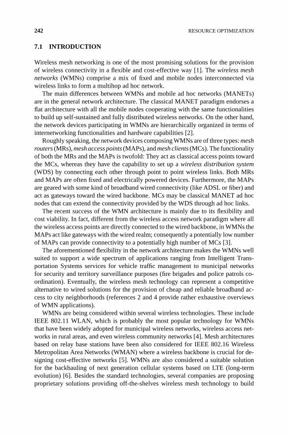
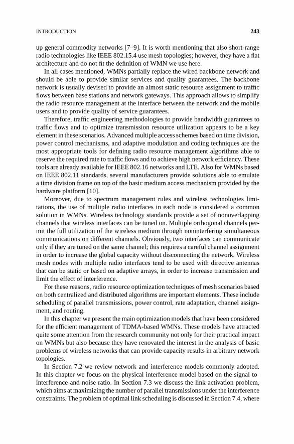
At every instant, transmitters can send information, provided that interferenceconstraints at receivers are satisfied. There are basically two interference models thathave been considered in the literature: the protocol model and the physical model,exemplified respectively in Figures 7.1 and 7.2.

The simplest model of interference, the protocol model, considers a couple oftransmissions over link (i, j) and (l, h) as interfering each other if and only if eitherthe Euclidian distance from i to h or from l to j is less than a given value, defined asinterference range. The effect of the interference is considered to be boolean: Nodesinterfere only if they are within the reciprocal interference range, that is, a receiver

n

m

h

i

j

l

v

w

Figure 7.1 Protocol interference model.

MAXIMUM LINK ACTIVATION UNDER THE SINR MODEL 245

n

m

h

i

j

l

v

w

Figure 7.2 Physical interference model.

can correctly decode the transmission if no active transmitter is within its interferencerange. However, this model does not account for the sum of several “distant” signalsthat, once summed up, cause a significant noise.

In the physical model, instead, given (i, j) ∈ A, node i transmits correctly to nodej if and only if the interference at the receiver j is below a given threshold. Usingthe physical model of interference, we have that the signal-to-interference-noise ratio(SINR) at the receiver j is

SINRij = Pigij

η + ∑l∈I\{i} Plglj

≥ γ (7.1)

where I is the set of active senders and γ is the smallest threshold to have a suc-cessful transmission. The sum at the denominator allows to count all the interferenceexperimented by the receiver.

Note that in order to have a link between the pair of nodes i and j, the SINRconstraint must be satisfied when the node i is the only sender in the network, that is,I \ {i} = ∅. Indeed, each arc (i, j) ∈ A must satisfy at least the signal-to-noise ratio:

SNRij = Pigij

η≥ γ (7.2)

7.3 MAXIMUM LINK ACTIVATION UNDER THE SINR MODEL

A fundamental problem is to determine the maximum number of interference-freeparallel transmissions, which is correlated to the maximum throughput the networkcan support.

Using the protocol model, it is possible to define a conflict graph H where there isa node for each link in the original network topology G, and there is an edge betweenany pair of interfering links. In this case, the maximum link activation problem isequivalent to finding a Maximum Independent Vertex Set, which is a notoriouslydifficult NP-hard problem [11].


In the case of the physical model, this problem can be formulated as an IntegerLinear Program as follows. Let xij be a 0–1 variable equals to 1 whenever node i

transmits to node j.

max∑

ij ∈ A

xij (7.3a)

s.t.∑

(i,j) ∈ A

xij +∑

(j,i) ∈ A

xji ≤ 1, ∀i ∈ N (7.3b)

Pigij

η + ∑l ∈ N,l /= i Plgljxlj

≥ γ xij, ∀(i, j) ∈ A (7.3c)

xij ∈ {0, 1}, ∀(i, j) ∈ A (7.3d)

The objective function (7.3a) maximizes the number of transmissions. Constraints(7.3b) impose that each node may either transmit or receive to/from another node, butnot both; these are known as half-duplex and unicast constraints. Constraints (7.3c)are the interference constraints that impose the ratio (7.1) on every active link. Thoughthis constraint is nonlinear, it can be linearized with standard techniques, resulting inthe following big-M constraint:

Pigij −∑

l∈N,l /= i

Plgljxlj ≥ ηγ − Mij(1 − xij) (7.4)

where Mij is a constant big enough to guarantee that the constraint holds wheneverxij = 0.

So far we have considered that each node i transmits with a fixed constant powerPi. However, if the power were a variable of the problem, it would be possible toincrease the number of parallel transmissions. For instance, close-by nodes couldtransmit using a lower level of power, yielding a lower interference to distant nodes.

Let pi be a continuous variable representing the transmission power of the node i.The transmission power can be at most equal to Pmax. Let yi be a 0–1 variableindicating whether the node i is transmitting to any other node. The problem of findingthe maximum number of parallel transmission with variable power is formulated asthe following Mixed Integer Linear Program:

max∑

(i,j)∈A

xij (7.5a)

s.t.∑

(i,j)∈A

xij +∑

(j,i)∈A

xji ≤ 1, ∀i ∈ N (7.5b)

pi ≤ Pmax∑

(i,j)∈A

xij, ∀i ∈ N (7.5c)

pigij

η + ∑l∈N,l /= i plglj

≥ γ xij, ∀(i, j) ∈ A (7.5d)

xij ∈ {0, 1}, ∀(i, j) ∈ A (7.5e)

pi ≥ 0, ∀i ∈ N (7.5f)

OPTIMAL LINK SCHEDULING 247

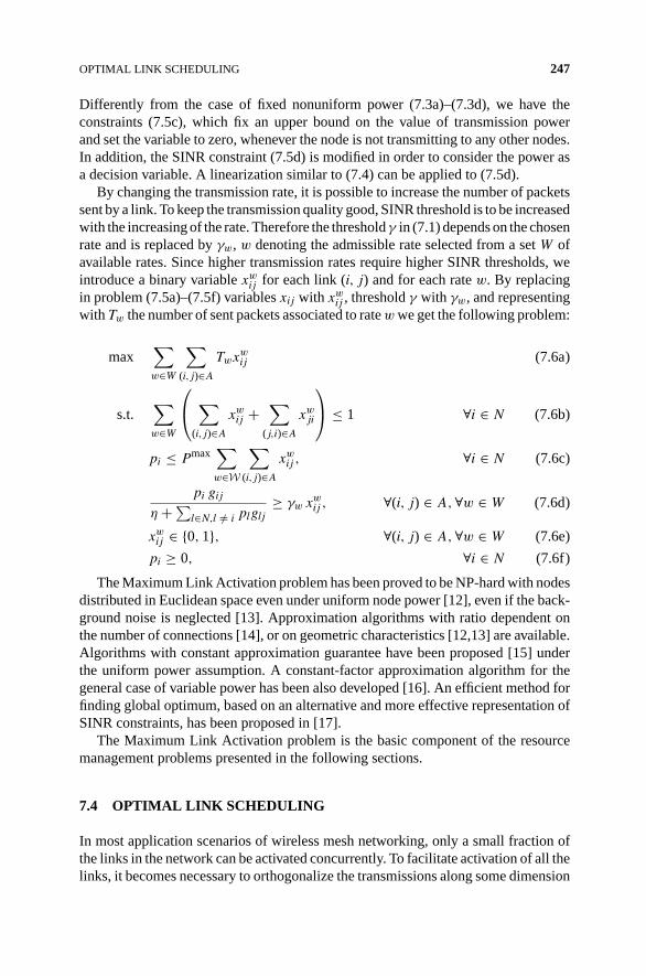
Differently from the case of fixed nonuniform power (7.3a)–(7.3d), we have theconstraints (7.5c), which fix an upper bound on the value of transmission powerand set the variable to zero, whenever the node is not transmitting to any other nodes.In addition, the SINR constraint (7.5d) is modified in order to consider the power asa decision variable. A linearization similar to (7.4) can be applied to (7.5d).

By changing the transmission rate, it is possible to increase the number of packetssent by a link. To keep the transmission quality good, SINR threshold is to be increasedwith the increasing of the rate. Therefore the thresholdγ in (7.1) depends on the chosenrate and is replaced by γw, w denoting the admissible rate selected from a set W ofavailable rates. Since higher transmission rates require higher SINR thresholds, weintroduce a binary variable xw

ij for each link (i, j) and for each rate w. By replacingin problem (7.5a)–(7.5f) variables xij with xw

ij , threshold γ with γw, and representingwith Tw the number of sent packets associated to rate w we get the following problem:

max∑

w∈W

∑

(i,j)∈A

Twxwij (7.6a)

s.t.∑

w∈W

⎛

⎝∑

(i,j)∈A

xwij +

∑

(j,i)∈A

xwji

⎞

⎠ ≤ 1 ∀i ∈ N (7.6b)

pi ≤ Pmax∑

w∈W

∑

(i,j)∈A

xwij , ∀i ∈ N (7.6c)

pi gij

η + ∑l∈N,l /= i plglj

≥ γw xwij , ∀(i, j) ∈ A, ∀w ∈ W (7.6d)

xwij ∈ {0, 1}, ∀(i, j) ∈ A, ∀w ∈ W (7.6e)

pi ≥ 0, ∀i ∈ N (7.6f)

The Maximum Link Activation problem has been proved to be NP-hard with nodesdistributed in Euclidean space even under uniform node power [12], even if the back-ground noise is neglected [13]. Approximation algorithms with ratio dependent onthe number of connections [14], or on geometric characteristics [12,13] are available.Algorithms with constant approximation guarantee have been proposed [15] underthe uniform power assumption. A constant-factor approximation algorithm for thegeneral case of variable power has been also developed [16]. An efficient method forfinding global optimum, based on an alternative and more effective representation ofSINR constraints, has been proposed in [17].

The Maximum Link Activation problem is the basic component of the resourcemanagement problems presented in the following sections.

7.4 OPTIMAL LINK SCHEDULING

In most application scenarios of wireless mesh networking, only a small fraction ofthe links in the network can be activated concurrently. To facilitate activation of all thelinks, it becomes necessary to orthogonalize the transmissions along some dimension


of freedom, such as frequency and time. In this section, we consider the task ofoptimally organizing link activation using a time division multiple access (TDMA)scheme. The resource unit in time is called timeslot. A timeslot can be used foractivation of multiple links, provided that they form a feasible solution to the link ac-tivation problem. In the baseline setting of the scheduling problem, each of the activelinks of a timeslot can transmit one packet. Intuitively, for the link activation problem,the solution tends to consist in links being spatially separated, because they generatelittle interference to each other. Thus the access scheme we consider can be viewed asa spatial reuse of the time resource. For this reason, the scheme is also referred to asspatial TDMA, or STDMA [18]. Although we will focus on computational optimiza-tion of STDMA, its worth noting that the STDMA capacity region has been studiedextensively also from an information-theoretical perspective (see, e.g., reference 19).

To characterize optimality in scheduling, a performance metric needs to be defined.An intuitive performance target is the minimization of the number of time slots ofthe schedule, subject to the constraint that the schedule meets the amount of trafficto be delivered on each link. If no traffic information on links is given (i.e., the MAClayer decision is completed decoupled from those of the high layers), the constraintis that every link appears at least once in the schedule. In this case, the schedulelength effectively represents the level of efficiency in resource reuse. The shorter theschedule length, the higher the efficiency. In addition, it is worth remarking that, whenscheduling is combined with packet routing (see the next section), which determinesthe amount of traffic on the links, the schedule length represents in fact the overallend-to-end delay. For these reasons, we will focus on minimum-length scheduling.Note that, using length as the performance target, scheduling deals with the groupingof links into subsets, one per timeslot. The order in which timeslots appear in theschedule is of no significance.

Performance study of link scheduling dates back to the introduction of multi-hop packet radio networks. We refer to references 20–23 for early developments ofheuristics, distributed computation, and approximation algorithms. A related prob-lem setting is to allocate timeslots to nodes for broadcast communications [24–26].In some of the references, the SINR consideration has been simplified to the protocolmodel; that is, nodes having a certain spatial separation (such as two hops and more)can transmit in the same timeslot.

The forthcoming discussion of link scheduling takes a mathematical programmingperspective. The goal is to derive the maximum achievable performance of STDMAin terms of schedule length [27–30]. To this end, we assume that there is no explicitrestriction on computing time, and information of the channel gain matrix is availble.Even with these two assumptions, solving the link scheduling problem is hard—thisis somewhat expected, since scheduling is a generalization of link activation, becauseit includes link activation as a subproblem.

7.4.1 Optimization Formulations

Let Rij denote the amount of traffic, in the number of packets, to be sent by link(i, j) ∈ A. We first examine a straightforward extension of the link activation


formulation (7.3) to multiple timeslots, assuming that the transmit power is given.Since there are R = ∑

(i,j)∈A Rij packets in total, a schedule of length R can accom-modate the traffic in the worst case. Denote by T = {1, . . . , R} the set containingR timeslots. To each timeslot t ∈ T , we associate a binary variable yt , representingwhether or not the slot is used in the schedule. A second set of binary variables xt

ij

augments the x-variables defined in Section 7.3 to timeslots; that is, xtij is one if link

(i, j) is active in slot t, otherwise it is zone. The scheduling problem can then beformulated using the following integer linear model.

min∑

t∈T

yt (7.7a)

s.t.∑

t∈T

xtij ≥ Rij, ∀(i, j) ∈ A (7.7b)

xtij ≤ yt, ∀(i, j) ∈ A, ∀t ∈ T (7.7c)∑

(i,j)∈A

xtij +

∑

(j,i)∈A

xtji ≤ 1, ∀i ∈ N, ∀t ∈ T (7.7d)

Pigij

η + ∑l∈N,l /= i Plgljx

tlj

≥ γ xtij, ∀(i, j) ∈ A, ∀t ∈ T (7.7e)

xtij ∈ {0, 1}, ∀(i, j) ∈ A, ∀t ∈ T (7.7f)

yt ∈ {0, 1}, ∀t ∈ T (7.7g)

The objective function (7.7a) minimizes the use of timeslots. By (7.7b), link (i, j)must appear at least Rij times in the schedule. Constraint (7.7c) connects the two setsof variables: Variable yt must be one (i.e., slot t is used), if any link (i, j) is activein the slot. The remaining constraints resemble those in (7.3) and extend the latter tomultiple timeslots using index t. The SINR constraints (7.7e) can be linearized in theway shown in (7.4).

Formulation (7.7) is compact: Both the numbers of variables and constraints arepolynomial in the size of the network. The major drawback of (7.7), in addition to theuse of big-M for linearizing (7.7e), is the presence of what is referred to as symmetryin integer programming [31]. Consider any scheduling solution that uses timeslot t1.Let t2 be any other timeslot, whether or not being present in the solution. Swappingthe values of the variables of t1 and t2 gives a solution that is equivalent to the originalone in terms of schedule length. Hence formulation (7.7) contains a huge numberof solutions that are seemingly different but in fact equivalent in performance. Theimpact of symmetry on computation is huge; in practice, solving (7.7) to optimalityis feasible only for networks of a small number of links.

The above discussion of symmetry also gives a hint for overcoming it. Becauseswapping the contents of timeslots has no effect on the quality of the schedule, we arenot interested in the indices of the timeslots used, but the contents of the them. Eachtimeslot in the schedule contains a subset of the links to be activated concurrently.Henceforth, we refer to such a subset of links—that is, a solution to the link activationproblem (7.3)—as a compatible set, or a configuration. Whereas the former is intuitive


for the scheduling problem under consideration, the latter is more accurate when weextend scheduling to rate adaptation.

Suppose, for a moment, that we do have access to the entire set S containing allthe compatible sets. A subset of links form an element s ∈ S if and only if they satisfythe constraints (7.3b)–(7.3d). Then, schedule amounts to select elements from S, anddetermine how much each of the selected elements should be used. Toward this end, weassociate an integer variable λs, s ∈ S, denoting the number of times that compatibleset s is used in the schedule, or, equivalently, the number of timeslots allocated tocompatible set s. To express the content of s, we define parameter aijs, which is oneif link (i, j) is active in compatible set s, and zero otherwise. The scheduling problemcan be formulated as the following integer program.

min∑

s∈S

λs (7.8a)

s.t.∑

s∈S

aijsλs ≥ Rij, ∀(i, j) ∈ A (7.8b)

λs ∈ Z+, ∀s ∈ S (7.8c)

The objective function (7.8a) represents the number of timeslots assigned for theoverall usage of the compatible sets. Constraints (7.8b) ensure that, for each link (i, j),the compatible sets containing the link together must have at least Rij timeslots in theschedule.

Instead of using parameter aijs, one can define set Sij ⊆ S to denote the subset ofcompatible sets containing link (i, j). With this set notation, constraints (7.8b) become∑

s∈Sijλs ≥ Rij, ∀(i, j) ∈ A. The reason for using parameter aijs in the formulation

above is that the parameter can alternatively be interpreted as the number of packets(zero or one in the basic scheduling problem) that link (i, j) transmits if one timeslot isassigned to set s; this interpretation is useful later in the discussion of rate adaptation.

7.4.2 Column Generation

Formulation (7.8) has much fewer constraints than (7.7). Also, the formulation doesnot model the SINR requirement (which is “hidden” in the construction of compat-ible sets). On the other hand, set S contains all compatible sets; thus the number ofvariables, or columns if (7.8b) is written in matrix form, is in general exponentialin network size. For this reason, a practical solution approach will have to make arestriction on the compatible sets to be considered. Preferably, the compatible setsincluded into the restricted formulation are likely those used in the optimal schedule.To this end, a systematic way is to apply a column generation method to the linearprogramming (LP) relaxation of (7.8). In LP, column generation is applicable if thenumber of variables is exponentially many; hence most of columns in the constraintmatrix are not explicitly available, but the structure of the problem allows for theconstruction of new and promising columns to be included in constraint matrix [32].The restricted problem, in which a small subset of all possible columns is kept, is


referred to as the master problem. By construction, the optimum of the master problemrepresents a feasible but not necessarily optimal solution to the original problem withthe full set of variables. Column generation uses the classical optimality condition ofthe simplex method, namely that the reduced costs of all variables must be nonnega-tive for minimization (and nonpositive for maximization). Calculating reduced cost isstraightforward in the classical simplex method. In column generation, in contrast, thecalculation of the variable having the smallest reduced cost (assuming minimization)is done via solving another auxiliary optimization problem, known as the subproblem.The subproblem is formulated so that its solution space corresponds to the completeset of columns (in our case, the compatible sets) in the original, unrestricted problem.From the solution of the subproblem, one either obtains a new column with favorablereduced cost to augment the master problem, or concludes no such column exists.The column generation method alternates between the master problem and the sub-problem, until the optimality condition is met. Typically, in comparison to the full setof columns, only a tiny fraction will be generated before optimality is reached.

Applying column generation to link scheduling, the master problem is definedby (7.8) with two modifications. First, the variables are continuous, that is, λs ∈ R+,

s ∈ S. Second, instead of the entire set S, a small subset S′ ⊂ S is used and augmentedsuccessively. Any S′ ⊂ S admitting feasibility of the master problem can serve asthe starting point. The simplest choice is to start with S′ = A; that is, single-linkcompatible sets corresponding to pure TDMA scheduling. For the subproblem, itis clear from the discussion above that the constraints are exactly those in the linkactivation problem (7.3). The objective function of the subproblem models reducedthe costs of compatible sets. By LP theory, for s ∈ S, the reduced cost of λs in (7.8) hasthe following form, where πij ≥ 0 denotes the dual variable associated with (7.8b).

cs = 1 −∑

(i,j) ∈ A

aijsπij (7.9)

The dual variable values originate from the optimum of the master problem overthe restricted set S′. Thus in the subproblem, we are looking for a compatible sets, to be represented by the x-variables in (7.7), that minimizes the reduced cost orequivalently, maximizes the sum in (7.9). In this sum, link (i, j) is associated withvalue πij or zero, depending on whether or not the link is active. We thus arrive at thefollowing formulation of the subproblem.

max∑

(i,j)∈A

πijxij (7.10a)

s.t. (7.3b) − (7.3d) (7.10b)

Formulation (7.10) is link activation with a weighted objective function. By itsdesign, column generation solves a sequence of link activation problems; this ismuch more efficient than constructing the contents of many compatible sets at once;see formulation (7.7). By alternating between solving the master problem and the


subproblem, the method decomposes the scheduling task into constructing compati-ble sets and optimizing their use.

Upon termination, the optimum LP of (7.8) may be fractional. In this case, theobjective function value bounds the integer optimum from below. To reach an integersolution in the λ-variables, one can apply an integer linear solver to (7.8) over theset of compatible sets available in the last iteration of column generation, or, if thistakes excessive computing time, a heuristic algorithm. In either case, there is noguarantee of global optimality, because some compatible sets in the integer optimummay not be present in the LP optimum. Ensuring global optimality would requirea branch-and-price technique of integer programming [31]. Empirically, however,for the scheduling problem, rounding the LP optimum leads to either the globallyoptimum, or a near-optimal approximate solution, which together with the LP valueform a very tight interval confining the optimum [27–29].

7.4.3 Extension to Power Control and Rate Adaptation

Having examined the basic model of link scheduling, let us consider extending theproblem setting to power control and rate adaptation. Because power control enlargesthe space of compatible sets, it can potentially reduce the number of timeslots in theoptimal schedule. When rate selection is enabled, the selection can be combined withthe power level, using a cross-layer design approach, to achieve additional perfor-mance gain [33–35]. A further extension is to include end-to-end routing, which willbe examined in the next section.

To enable power control in formulation (7.7), one needs to introduce continuousvariables pt

i, i, ∈ N, t ∈ T , to denote the power of node i in timeslot t. Following thetreatment of variable power in Section 7.3, the extension of formulation (7.7) to powercontrol is straightforward: We replace Pi in (7.7e) with power variable pt

i, and addpt

i ≤ Pmaxyti, ∀i ∈ N, ∀t ∈ T , which extends (7.5c) to timeslots.

Consider formulation (7.8). Power control has no impact on the definition of thevariables or constraints, simply because the construction of compatible sets is notpart of the formulation. The column generation method remains applicable. The sub-problem, however, has to be modified to incorporate power control, that is, to use theconstraints of the variable-power link activation problem (7.5b)–(7.5f) in Section 7.3.

Next, we take a further step of problem extension by including rate adaptation. Theaspect originates from the use of multiple modulation and coding schemes (MCSs).Each MCS corresponds to a rate and an SINR threshold for that rate. Let W denote theset of MCSs. For each w ∈ W , we use Tw to denote the number of packets supportedby the rate in a timeslot, and we use γw to denote the SINR threshold. Note that,with rate adaptation, the information defining a timeslot consists in not only the linksbeing active, but also their rates in terms of the number of packets. For this reason,it is more convenient to call the content of a timeslot a configuration rather than acompatible set.

For formulation (7.7), incorporating rate adaptation amounts to extending the def-inition of the x-variables with another index representing the rate, that is, xwt

ij equalsone, if and only if link (i, j) transmits in slot t with rate w of Tw packets. The following


inequality extends the demand constraint (7.7b) by an additional sum over the ratesto account for the number of packets of each rate level.

∑

t∈T

∑

w∈W

Twxwtij ≥ Rij, ∀(i, j) ∈ A (7.11)

Adapting constraints (7.7c)–(7.7d) to rate adaptation is done by including asum over the rates. For example, (7.7c) is replaced by

∑w∈W xwt

ij ≤ yt, ∀(i, j) ∈ A,

∀t ∈ T . Note that the inequality implies also∑

w∈W xwtij ≤ 1; that is, at most one rate

can be used for each link and timeslot. For (7.7d), the modification is analogous.A straightforward (but naive) way of defining the SINR constraint with rate adap-

tation is to introduce one inequality of type (7.5d) for each link, timeslot, and ratelevel. As a result, in comparison to (7.7e), the number of SINR constraints grows byfactor |W |. However, utilizing the aforementioned property that at most one of theterms in

∑w∈W xwt

ij equals one, we can, in fact, replace the x-variable in (7.7e) with∑

w∈W xwtij to formulate the SINR requirement, without any increase in the number of

constraints. Thus the counterpart of (7.7e) for rate adaptation has the following form:

ptigij

η +∑

l∈N,l /= i

ptlglj

∑

w∈W

xwtlj

≥∑

w∈W

γw xwtij , ∀(i, j) ∈ A, ∀t ∈ T (7.12)

Even though the number of SINR constraints (7.12) is the same as that of (7.7e),the extended formulation of (7.7) for rate adaptation is harder to solve, because ofthe increase in the number of variables to model rates and continuous power. Hencethe extended formulation admits optimal or near-optimal solution for network of verysmall size only.

Let us now use the notion of configurations to formulate scheduling with rateadaptation, by adapting (7.8). To this end, S is used to denote the set of all feasibleconfigurations. We augment the meaning of the a-parameters, and define aijs = Tw,if link (i, j) is active with rate w ∈ W in configuration s ∈ S. If the link is not ac-tive at all in s, we let aijs = 0. The λ-variables are reused. With the new definition ofthe a-parameters, formulation (7.8) remains valid for scheduling with rate adaptation.Consider applying the idea of column generation, as described in Section 7.4.2. The re-duced cost expression (7.9) does not change. For a configuration s, the contribution oflink (i, j) in (7.9) is either zero if the link is not active, or the rate (in the number of pack-ets) scaled with the dual variable πij . Reusing the variable definition in Section 7.3, theobjective function of the column generation subproblem has the following expression.

max∑

(i,j)∈A

∑

w∈W

πijTwxwij (7.13)

The constraints of the subproblem together shall define the space of feasible config-urations. Hence constraints (7.6b) and (7.6c) are both present. The SINR constraintsare obtained by skipping the slot index t in (7.12). The SINR constraints are obtainedby skipping the slot index t in (7.12). By solving this new version of the subproblem,


the column generation approach in Section 7.4.2 can be used for link scheduling withrate adaptation. It has been observed that the approach is able to effectively deliverthe optimal or a near-optimal solution for network size of practical interest [29].

7.5 JOINT ROUTING AND SCHEDULING

In the link scheduling problem presented in the previous section, the traffic on everylink was assumed to be given. However, in practice, link loads are defined by routingpaths. The routing of traffic demands in the network is another parameter we cantune in order to optimize the performance: routing determines transmitting nodesand the number of packets sent by each of these nodes. Transmitting nodes and thenumber of their transmissions, in turn, influence the global interference. Therefore,the optimal scheduling is affected by routing decisions, and this dependence makesthe joint routing and scheduling optimization a further step toward the improvementof the network performance.

In this section, we consider, in addition of link scheduling, the optimization prob-lem of routing a set of traffic demands, each having a source node and a destinationnode. Most of the common routing protocols are based on shortest paths. The shortestpath is a routing assumption that is made for the sake of simplicity, however, it maynot lead to the best possible performance due to the imposed, but not necessarilyneeded, constraint of selecting only shortest paths. In many cases, it can even gen-erate heavy-loaded bottleneck links. In order to obtain the real achievable optimum,the shortest path simplification must be dropped and the optimization approach mustassume a global perspective.

Leveraging routing and link activation, the goal is to provide the shortest framethat allows to deliver the required number of packets from the source node to thedestination. Note that the slot order is not important as we are not concerned withbuffering limits. Indeed, it is not required that the specific packet is transferred fromsource to destination in the same frame, but rather, that d packets of a given flow aresent by the transmitter and received by the destination within a frame. This meansthat received packets could have been transmitted in previous frames and deliveredalong the path like a pipeline. A simple example is shown in Figure 7.3, where thedemand is a single packet from node A to node B within a frame. Even if the linkactivation is out of order, after a negligible transient state, the scheduling satisfies therequest of one packet delivered per frame.

Since each slot of the frame must still be a feasible configuration, the approachof the previous section can be easily adapted to joint routing and scheduling op-timization, thanks to the separation provided by the column generation algorithm.Technological constraints which define the set of simultaneously active links do notchange, therefore the subproblem which generates compatible sets remains the same.The master problem that optimizes the use of such compatible sets, instead, must bemodified in order to take into account the additional routing issues. An approach deal-ing with joint routing and scheduling adopting this strategy was presented in reference36. Various other approaches to this problem were presented in references 37–41.

JOINT ROUTING AND SCHEDULING 255

Figure 7.3 Example of out-of-order scheduling.

In the following, we briefly review the key differences from the basic link schedul-ing problem.

7.5.1 Routing via Flow Conservation

Let the traffic demands be represented by a set of triplets D = {〈o, t, d〉 | o, t ∈ N,

d ∈ Z+}, where each triplet 〈o, t, d〉 indicates the number of packets d to be routedfrom node o to node t. In order to formulate the routing problem, we need to introduceadditional flow variables to the master problem (7.8a)–(7.8c). Let f k

ij be a flow variable

indicating the number of packets of demand 〈ok, tk, dk〉 routed over link (i, j) for thekth traffic demand. The problem of routing and scheduling the traffic demand set D

is formalized as follows:

min∑

s∈S

λs (7.14a)

s.t.∑

(i,j)∈A

f kij −

∑

(j,i)∈A

f kji =

⎧⎪⎨

⎪⎩

dk, i = ok

−dk, j = tk

0, otherwise

∀i ∈ N, ∀k ∈ D (7.14b)

∑

s∈Sij

λs ≥∑

k∈D

fkij ∀(i, j) ∈ A (7.14c)

f kij ∈ Z+ ∀(i, j) ∈ A, ∀k ∈ D (7.14d)

λs ∈ Z+ ∀s ∈ S (7.14e)


The objective function (7.14a) minimizes the number of timeslots. Constraints (7.14b)are the routing constraints imposing flow balance at every node i, for each demand k.Constraints (7.14c) impose that every link (i, j) is assigned to a number of timeslotsat least equal to the number of times the link is used for routing any demand, while(7.14d) and (7.14e) are integrality constraints.

Note that the set of configurations S is the same as defined in Section 7.4.1.Therefore, as long as we tackle this problem via the column generation approach asused for the link scheduling problem, we can easily deal with the problem of jointrouting and scheduling with fixed power, variable power, and rate adaptation. Themain difference will be in the solution of the master problem.

7.5.2 Routing via Path Generation

Since in problem (7.14) the number of flow variables and flow balance constraintsmight become significant, the problem of joint routing and scheduling can be formu-lated with a slightly different formulation that uses path variables instead of link flowvariables. This formulation was originally proposed and evaluated in reference 42.

Let H be the set of all possible paths between any pair of nodes in G. The idea isto introduce a path integer variable βp for every path p ∈ H that indicates the numberof packets that routed on path p. Let Hij be the subset of paths that pass through link(i, j) and let H〈o,t〉 be the subset of paths that start from node o and ends to node t.Then the master problem can be reformulated as

min∑

s∈S

λs (7.15a)

s.t.∑

p∈H〈o,t〉

βp ≥ dk, ∀〈o, t, d〉 ∈ D (7.15b)

∑

s∈Sij

λs ≥∑

p∈Hij

βp, ∀(i, j) ∈ A (7.15c)

βp ∈ Z+, ∀p ∈ H (7.15d)

λs ∈ Z+, ∀s ∈ S (7.15e)

Constraints (7.15b) ensure that for each demand at least d paths from its sourceo to the destination t are selected. Constraints (7.15c) ensure that there are enoughconfigurations according to the number of paths used to route the traffic demands.

Note that the number of paths in H is exponential, but we can start with an initialset of paths and then we can use an additional pricing subproblem to generate onlyinteresting paths—that is, paths of negative reduced costs. The problem of generatingnegative reduced cost path can be formulated as a shortest path problem, wherethe arc costs are given by the dual multipliers associated with (7.15c). The shortestpath problem must be solved for each demand, with an additional fixed cost givenby the dual multipliers of constraints (7.15b). As long as a single path of negativereduced cost exists, the column generation algorithm iterates. Additional technicaldetails on how to solve the routing problem with both path and configuration pricing

DEALING WITH CHANNEL ASSIGNMENT AND DIRECTIONAL ANTENNAS 257

subproblems can be found in reference 42, where the authors have applied this ideato the problem of joint routing and scheduling in wireless mesh networks with theprotocol interference model.

7.6 DEALING WITH CHANNEL ASSIGNMENTAND DIRECTIONAL ANTENNAS

As clearly emerging from previous sections, the spatial reuse of the time resource isa critical aspect for the performance of a WMN. Roughly speaking, the more activelinks configurations have, the better throughput the system can achieve.

The main obstacle that prevents the simultaneous activation of many links in theSINR model is the interference on the receiver caused by other concurrent transmis-sions. Advanced physical layers can help in reducing the effect of the interference.Besides using robust modulations and codings or high-quality components allowingtransmission decoding at low SINRs, a great help comes from the use of advancedantenna systems.

A further reduction of interference effect, resulting in a performance boost, can beobtained in multiradio multichannel scenario. With the development of new and on-the-shelf wireless equipment, the use of multiple radio interfaces in each node is nowconsidered a common solution in WMNs. In addition, wireless technology standardsprovide an RF spectrum with a set of nonoverlapping channels wireless interfaces canbe tuned on. Multiple orthogonal channels permit the full utilization of the wirelessmedium through noninterfering simultaneous communications on different channels.Obviously, two interfaces can communicate only if they are tuned on the same channel,this requires a careful channel assignment in order to increase the global capacitywithout disconnecting the network. Effects of multiple interfaces on network capacityin presence of multiple channels have been theoretically analyzed [35], and severalsolutions of the channel assignment problem have been proposed [43–48].

In the following we present a channel assignment approach that is built on topof the solution given by the models either in Section 7.4 or in Section 7.5. It tightlyintegrates with the approach adopted so far and can be seen as a block of the presentedmodular framework.

7.6.1 Channel Assignment

To model and solve the channel assignment problem, we leverage the features of theproblem formulations proposed in the previous sections, which are based on sets ofcompatible simultaneous transmissions, called configurations. The general approachis to assign configurations to available channels, taking into account constraints dueto device characteristics [49].

Each network node is equipped with a given number of wireless interfaces, and eachof them can be tuned on a single channel selected from a set of orthogonal channels.According to the hardware and software characteristics of nodes and wireless cards,two channel assignment strategies can be considered:


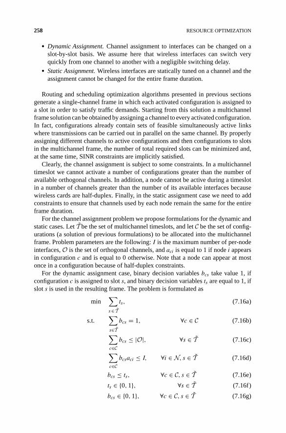
• Dynamic Assignment. Channel assignment to interfaces can be changed on aslot-by-slot basis. We assume here that wireless interfaces can switch veryquickly from one channel to another with a negligible switching delay.

• Static Assignment. Wireless interfaces are statically tuned on a channel and theassignment cannot be changed for the entire frame duration.

Routing and scheduling optimization algorithms presented in previous sectionsgenerate a single-channel frame in which each activated configuration is assigned toa slot in order to satisfy traffic demands. Starting from this solution a multichannelframe solution can be obtained by assigning a channel to every activated configuration.In fact, configurations already contain sets of feasible simultaneously active linkswhere transmissions can be carried out in parallel on the same channel. By properlyassigning different channels to active configurations and then configurations to slotsin the multichannel frame, the number of total required slots can be minimized and,at the same time, SINR constraints are implicitly satisfied.

Clearly, the channel assignment is subject to some constraints. In a multichanneltimeslot we cannot activate a number of configurations greater than the number ofavailable orthogonal channels. In addition, a node cannot be active during a timeslotin a number of channels greater than the number of its available interfaces becausewireless cards are half-duplex. Finally, in the static assignment case we need to addconstraints to ensure that channels used by each node remain the same for the entireframe duration.

For the channel assignment problem we propose formulations for the dynamic andstatic cases. Let T be the set of multichannel timeslots, and let C be the set of config-urations (a solution of previous formulations) to be allocated into the multichannelframe. Problem parameters are the following: I is the maximum number of per-nodeinterfaces, O is the set of orthogonal channels, and aci is equal to 1 if node i appearsin configuration c and is equal to 0 otherwise. Note that a node can appear at mostonce in a configuration because of half-duplex constraints.

For the dynamic assignment case, binary decision variables bcs take value 1, ifconfiguration c is assigned to slot s, and binary decision variables ts are equal to 1, ifslot s is used in the resulting frame. The problem is formulated as

min∑

s ∈ T

ts, (7.16a)

s.t.∑

s∈Tbcs = 1, ∀c ∈ C (7.16b)

∑

c∈Cbcs ≤ |O|, ∀s ∈ T (7.16c)

∑

c∈Cbcsaci ≤ I, ∀i ∈ N, s ∈ T (7.16d)

bcs ≤ ts, ∀c ∈ C, s ∈ T (7.16e)

ts ∈ {0, 1}, ∀s ∈ T (7.16f)

bcs ∈ {0, 1}, ∀c ∈ C, s ∈ T (7.16g)


Note that in the above formulation, channels are not explicitly identified. We justneed to ensure that the number of used channels is compatible with problem pa-rameters thanks to the ability of wireless interfaces to switch from one channel toanother. Constraints (7.16b) guarantee that each configuration is assigned to a slot.Constraints (7.16c) and (7.16d) force respectively the maximum number of avail-able orthogonal channels and maximum number of per-node interfaces. Constraints(7.16e) regulate multichannel timeslot activation. A feasible channel assignment canalways be obtained by assigning one of the available channels to each configura-tion in a multichannel timeslot, because constraints (7.16c) guarantee the processcorrectness.

The static assignment problem is a more constrained and complex problem, andchannels assigned to configurations must be explicitly identified in order to ensurethat channel assignment to nodes does not change from slot to slot. To this pur-pose, new binary variable sets must be introduced, in addition to ts. Variables b

fcs

are equal to 1 if configuration c is assigned to slot s with channel f , and vari-ables rif take value 1 if node i uses channel f . The static assignment problem isformulated as

min∑

s∈Tts, (7.17a)

s.t.∑

s∈T

∑

f∈Obfcs = 1, ∀c ∈ C (7.17b)

∑

c∈Cbfcs ≤ 1, ∀s ∈ T,∀f ∈ O (7.17c)

∑

c∈C

∑

f∈Obfcs ≤ |O|, ∀s ∈ T (7.17d)

rif ≥∑

s∈Tbfcsaci, ∀i ∈ N, ∀c ∈ C, ∀f ∈ O (7.17e)

∑

f∈Orif ≤ I, ∀i ∈ N (7.17f)

bfcs ≤ ts, ∀c ∈ C, s ∈ T, f ∈ O (7.17g)

bfcs ∈ {0, 1} , ∀c ∈ C, ∀s ∈ T,∀f ∈ O (7.17h)

rif ∈ {0, 1} , ∀i ∈ N, ∀f ∈ O (7.17i)

where O is the set of orthogonal channels. Constraints (7.17b), (7.17d), (7.17f), and(7.17g) have respective equivalents in the dynamic assignment problem. We addconstraints (7.17c), which state that in each multichannel timeslot we can assign atmost one configuration per channel and constraints (7.17e) that allow to count thenumber of channels assigned to a node within the frame. The number of assignedchannels is equal to the number of interfaces to be installed.


Figure 7.4 Channel assignment heuristic algorithm.

A heuristic algorithm can be implemented using the admissibility version of thechannel assignment problem. We focus, without loss of generality, on the static as-signment formulation in (7.17). This admissibility version is a problem where theobjective function (7.17a) is removed along with constraints (7.17g) and ts variables,and a fixed number of multichannel timeslots is introduced. The goal is to find afeasible solution that exactly uses the given number of multichannel timeslots andsatisfies all the constraints. Clearly, the complexity of this version is not greater thanthe optimization version, and it usually runs in short time.

The flow chart of our heuristic algorithm is reported in Figure 7.4, where theupper bound on the number of multichannel time slots of the final frame is defined asUB = |C|

Iand the related lower bound as LB = |C|

|O| . The upper bound derives fromthe maximum number of per-node interfaces: A solution where in each timeslot onlyI configurations are present is always feasible because a node is active at most in I

channels per slot. The lower bound, instead, is motivated by the fact that, by relaxingconstraints on the maximum number of interfaces, at most |O| configurations can beassigned to a slot.

The algorithm starts solving the admissibility problem with a number of multi-channel timeslots equal to UB and, if a feasible solution is found, this number isiteratively decreased by one. Otherwise, if the problem with that number of time-slots is infeasible, execution is stopped. This means that, provided that the previousiteration ended with a feasible solution, its number of timeslots is also optimal. Theexecution time of both the single iteration and the total algorithm have two time lim-its, respectively, TITER and TTOT in order to obtain at least one suboptimal solutionwithin TTOT.


7.6.2 Directional Antennas

Technology solutions based on directional antenna for WMNs has been widely studieddue to the potential high-performance improvement [50]. The main advantage of usingdirectional antennas with wireless multihop networks is the reduced interference andthe possibility of having parallel transmissions among neighbors with a consequentincrease of spatial reuse of radio resources.

Directional antennas allow the concentration of the transmitted energy into alimited region and a higher reception gain from certain arriving directions. As aconsequence, the transmitter can limit the interference generated at nonintended re-ceivers and, similarly, a receiver can attenuate the interference power coming fromnonintended transmitters. The interference reduction permits a higher channel reusewith respect to omnidirectional antennas, leading to better resource exploitation andpotentially better performance.

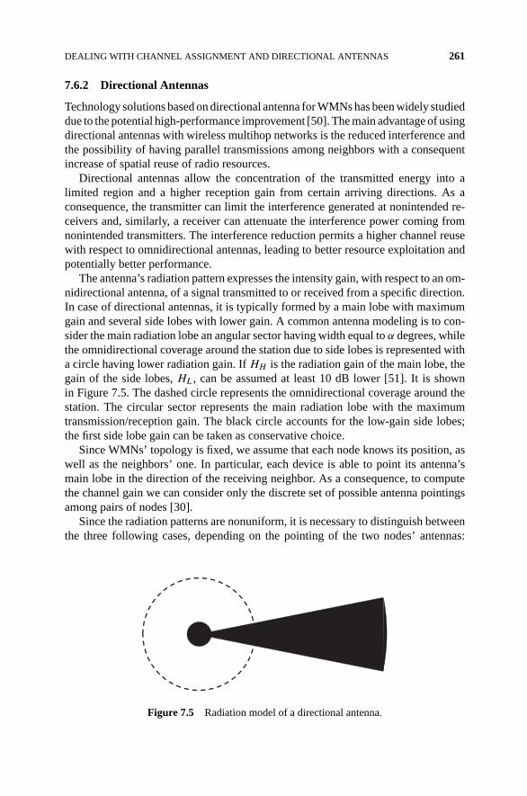
The antenna’s radiation pattern expresses the intensity gain, with respect to an om-nidirectional antenna, of a signal transmitted to or received from a specific direction.In case of directional antennas, it is typically formed by a main lobe with maximumgain and several side lobes with lower gain. A common antenna modeling is to con-sider the main radiation lobe an angular sector having width equal to α degrees, whilethe omnidirectional coverage around the station due to side lobes is represented witha circle having lower radiation gain. If HH is the radiation gain of the main lobe, thegain of the side lobes, HL, can be assumed at least 10 dB lower [51]. It is shownin Figure 7.5. The dashed circle represents the omnidirectional coverage around thestation. The circular sector represents the main radiation lobe with the maximumtransmission/reception gain. The black circle accounts for the low-gain side lobes;the first side lobe gain can be taken as conservative choice.

Since WMNs’ topology is fixed, we assume that each node knows its position, aswell as the neighbors’ one. In particular, each device is able to point its antenna’smain lobe in the direction of the receiving neighbor. As a consequence, to computethe channel gain we can consider only the discrete set of possible antenna pointingsamong pairs of nodes [30].

Since the radiation patterns are nonuniform, it is necessary to distinguish betweenthe three following cases, depending on the pointing of the two nodes’ antennas:

Figure 7.5 Radiation model of a directional antenna.


(a) The two nodes have the main lobe reciprocally pointed, (b) they both have themain lobe pointed away from the other node, (c) one node has the main lobe pointedtoward the other one while the main lobe of the other node is pointed away from thefirst node. Let gij be the channel gain due to propagation attenuation between nodesi and j; the channel gain matrix is

Hj � ri � q = gij ·

⎧⎪⎨

⎪⎩

HHHH if case (a) occurs

HLHL if case (b) occurs

HHHL if case (c) occurs

where q is the node pointed by the transmitting antenna at node i and r is the nodepointed by the receiving antenna at j. Note that given the position of nodes i, q, j, r

and the angular width of the main lobe sector, the actual values of Hj � ri � q can be

precomputed for all nodes.Note that the use of directional antennas only impacts on channel gains and their

presence influences only SINR constraints. In case of fixed transmission power, con-straints (7.3c) become

PiHj � ii � j

η +∑

(l,m)∈A,l /= i,

PlHj � il � mxlm

≥ γ xij, ∀(i, j) ∈ A (7.18)

The first channel gain term, Hj � ii � j derives from the fact that an active link (i, j)

implies the antennas of nodes i and j being reciprocally pointed. Similarly, in thesecond term, Hj � i

l � m, the transmitting node l’s antenna is pointed to the receiving nodem since each interfering active link (l, m) is taken into consideration. Finally, note that,differently from the previous formulations where antennas are isotropic, the power ofthe interfering transmitting node alone is not sufficient to compute the interference.Indeed, with directional antennas, it is also important where the antenna is pointedand, thus, which is the destination of the interfering transmission. As a consequence,in case of scenarios with power control, constraints (7.5c), (7.5d), and (7.5f) must bemodified into

pij ≤ Pmaxxij, ∀(i, j) ∈ A (7.19a)

pijHj � ii � j

η +∑

(l,m)∈A,l /= i,

plmHj � il � m

≥ γ xij, ∀(i, j) ∈ A (7.19b)

pij ≥ 0, ∀(i, j) ∈ A (7.19c)

COOPERATIVE NETWORKING 263

where the power variable pij captures both the transmitting power and the destinationof the transmission. Similary, when rate adaptation is available as well we obtain

pij ≤ Pmax∑

w∈Wxwij , ∀(i, j) ∈ A (7.20a)

pijHj � ii � j

η +∑

(l,m)∈A,l /= i,

plmHj � il � m

≥ γw xwij , ∀(i, j) ∈ A (7.20b)

pij ≥ 0, ∀(i, j) ∈ A (7.20c)

7.7 COOPERATIVE NETWORKING

A recent line of research deals with multihop wireless networks where the devicescooperate to transmit the same information [52]. This is different from all the prob-lems presented up to here, since previously we had the implicit assumption that atransmission involves exactly one sender and one receiver. With cooperative net-working, we could have two or more devices that transmit the same packet. In thiscase, the receiver can combine all the received signals and improve the signal to noiseratio. Therefore, cooperative networking can lead to more reliable transmissions. Inaddition, if a receiver is too far away from the other devices to correctly receive thesignal of a single transmitter, it might be the case that by combining the signals oftwo or more transmitters, the overall signal becomes strong enough (or stronger ofthe noise), and the communication can be established.

In the following, we present a formalism that allows to adapt with a minimal effortall the models presented in this chapter to the case of cooperative networking. In-depthdetails along with computational results that compare standard ad hoc networks withcooperative ad hoc networks are presented in reference 53.

7.7.1 κ-Cooperation Graph

Network model is based on the concept of level of cooperation.

Definition 1. A wireless network G has a κ-level of cooperation if, during thesame timeslot, at most κ nodes are allowed to transmit the same packet to a set ofone or more receiving nodes, and each receiver can combine the packets from the κ

transmitters.

For κ > 1, graph G is not sufficient for modeling cooperative transmission. Wedevelop a graph concept, which we refer to as the κ-Cooperation graph, to generalizethe original topology G.

Definition 2. For graph G = (N, A), the κ-Cooperation Graph Gκ = (Nκ, Aκ), isthe auxiliary graph representing all possible transmissions in G permitted by a κ-level


i

(i)

(i, j)

( j)

j

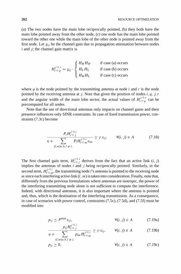
Figure 7.6 An illustration of supernodes and superlink.

of cooperation. A node i ∈ Nκ represents a nonempty subset of N having cardinalityup to κ, and a link (i, j) ∈ Aκ represents simultaneous transmissions of one packetfrom all nodes in the i’s node set in N to j’s node set in N.

For the sake of clarity, we use v and w to denote nodes in the original graph G, and i

and j nodes in the cooperation graph Gκ. Nodes and links in Gκ are also referred to assupernodes and superlinks. Let (i) denote the set of nodes in N forming supernodei in Nκ, and (i, j) the set of links forming superlink (i, j) ∈ Aκ: (i, j) = {(v, w) |v ∈ (i), w ∈ (j)}. Note that the size of Gκ grows exponentially in κ. When κ = 1,the κ-cooperation graph Gκ reduces to the original topology G. The concepts ofsupernode and superlink are illustrated in Figure 7.6. In this example, each of thetwo supernodes i and j contains two nodes in N, and the superlink (i, j) representstransmissions from all nodes in (i) to all nodes in (j).

In Figure 7.6, the four transmissions do not necessarily correspond to links inthe original graph G. This is because the SNR condition takes a new form in thecooperation graph Gκ. For a superlink (i, j) ∈ A to exist, the following SNR conditionapplies to all receivers of the superlink; that is, for all w ∈ (j) we obtain

SNRiw =∑

v∈(i) Pvgvw

η≥ γ. (7.21)

The numerator in (7.21) models the fact that the nodes (i) are transmitting thesame packet and hence all contributing to improving SNR. For this reason, a superlinkcan be established, as a result of cooperation, even if some or possibly none of thetransmissions of this superlink is part of the link set in the original topology.

When several supernodes are transmitting in the same timeslot, interference mustbe accounted for. Suppose, in addition to i, a set of supernodes � are transmitting inthe same timeslot. The SINR condition for superlink (i, j) is that for all w ∈ (j), thefollowing inequality holds:

SINRiw =∑

v∈(i) Pvgvw∑

l∈�

∑u∈(l) Puguw + η

≥ γ (7.22)

In (7.22), all nodes composing the supernodes in � generate interference to su-perlink (i, j). Note that a node u ∈ N may appear at most once in the denominator,


because the supernodes transmitting in any time slot all must have mutually disjointsets of nodes in the original graph.

7.7.2 Classes of Superlinks

The supernodes in Gκ vary in the cardinality of associated subsets of nodes in theoriginal graph. Based on this cardinality, we define four classes of superlinks.

1. One-to-One. These are the links in the original physical topology—that is,links in A. Superlink (i, j) is of this class if it satisfies the condition (i) = {v},(j) = {w}, and (v, w) ∈ A.

2. One-to-Many. A superlink of this class corresponds to a group of links in A orig-inating from the same node in N. Thus (i, j) ∈ Aκ is a one-to-many superlink if(i) = {v}, |(j)| > 1, and (v, w) ∈ A for all w ∈ (j). The one-to-many linksare also referred to as broadcast links. A special subclass of one-to-many linksis the so called buffering links, in which a node behaves as if it were transmittingalso to itself.

3. Many-to-One. A superlink (i, j) ∈ Aκ is of class many-to-one, if |(i)| > 1and (j) = {w}, w ∈ N \ (i). This superlink represents simultaneous trans-missions of the same packet from all nodes in (i) to the single receiver w in(j). A many-to-one link does not necessarily consist in a group of links in theoriginal graph; that is, (i) may contain node v for which (v, w) /∈ A, providedthat the SNR at w satisfies (7.21) by cooperation. Links in the many-to-oneclass are also referred to as cooperating links.

4. Many-to-Many. This class of links represent transmissions of the same packetbetween multiple transmitters and receivers in the original graph. A superlink(i, j) is a many-to-many link if and only if |(i)| > 1 and |(j)| > 1. Thesuperlink shown in Figure 7.6 is of this class. Similar to many-to-one superlinks,a many-to-many superlink (i, j) can be created by cooperation; hence it mayhave transmissions between one or multiple pairs of nodes v ∈ (i) and w ∈(j) for which (v, w) /∈ A. Many-to-many superlinks are also called broad-cooperating links or multicasting links.

Example 7.1. Figure 7.7 shows the physical topology of a wireless network with 5nodes. Figure 7.8 shows the supernodes of the corresponding 2-cooperation network.For clarity, only a few of the superlinks are drawn. The dot–dashed links are ofclass one-to-one; these are the links incident to node 2 in the original topology.The solid superlinks are broadcasting links from node 3 to supernodes {1, 2}, {1, 5},and {2, 5}, respectively. Each of the three dotted superlinks is a cooperating link,representing simultaneous transmissions of a packet from supernode {2, 3} to a singlereceiver. Note that transmissions on (2, 1), (2, 5), and (3, 4) do not correspond toany physical link in Figure 7.7. Finally, the dashed superlinks are multicasting links,each of which carries transmissions involving two transmitters and two receivers;some of these transmissions occur between nodes that do not have links in Figure 7.7.


1

5

3

2

4

Figure 7.7 Topology of a very simple wireless network.

1 {1,2} {1,3} {1,5}{ } { } { }

2 {2, 4} {2,5}

3 {3, 4} {3,5}

4{2,3} {4,5}

5{1,4}

Figure 7.8 A selection of supernodes and some superlinks of the 2-cooperation graph gen-erated from the network of Figure 7.7.

The distance in hops between a source–destination pair may benefit from cooperatingand multicasting links. For example, the shortest path from node 4 to node 1 has threehops if no cooperation is allowed. The shortest path distance in the cooperation graphbecomes two hops, and one of such paths is formed by 4, {2, 5}, and 1.

Example 7.2. A clear advantage of cooperative relaying consists in allowing thecommunication between nodes that, due to the SNR constraint, are not connected inthe original network. Figure 7.9 shows a small example of a network with 6 nodes andtwo demands 〈2, 4〉 and 〈4, 3〉. In the example, a demand represents a single packetassociated with a source and a destination. The transmission power P is 0.2 mW, thethermal noise at the receiver η is 10−10 mW, and the SNR threshold γ is 10. Sincenode 4 is disconnected from both node 2 and node 3, the two demands cannot be


1

23 4

(a)

(b)

5

6

2 → 3, 5 3, 5 → 4 4, 6 → 3 4 → 4, 6

Figure 7.9 Cooperative networking to provide additional connectivity. (a) Topology withP = 0.2 mW, η = 10−10 mW, γ = 10. (b) Routing and scheduling two demands 〈2, 4〉 and〈4, 3〉.

satisfied without cooperation. If we allow a 2-level of cooperation, the demand 〈2, 4〉is satisfied with the configurations 2 → {3, 5} and {3, 5} → 4, and the demand 〈4, 3〉is satisfied with the configurations 4 → {4, 6} and {4, 6} → 3. Note that the seconddemand uses the buffering link 4 → {4, 6}.

Example 7.3. The advantage of cooperation tends to decrease as the connectivityof the network increases. To quantify the connectivity, we use two network properties:(i) the network density δ = |A|

|N|(|N|−1) , that is, the percentage of links that satisfy theSNR constraint with respect to a fully connected network, and (ii) the network diame-ter , that is, the maximum hop distance between any pair of nodes. Figures 7.10 and7.11 show two networks that differ only in the level of connectivity. In the first case thenodes transmit withP = 0.1 mW. In the second case, the powerP is 0.4 mW. In this ex-ample, each pair of nodes i and j has a single-packet demand in both directions, that is,〈i, j〉 and 〈j, i〉. For the network of Figure 7.10, the optimal solution requires 130 times-lots without cooperation, and only 110 timeslots with cooperation, showing a clearadvantage of cooperation. In contrast, for the network of Figure 7.11 where the connec-tivity is much higher, the optimal schedule length is 74, with or without cooperation.

7.7.3 Column Generation Applied to κ-Cooperation

For the sake of brevity, we discuss here only the master problem and the pricing sub-problem of the problem of joint routing and scheduling in cooperative networking. Allthe general concepts and definitions about column generation were already presentedin the previous pages. Additional details are given in reference 53.


1

2

3

4

5

6

7

8

Figure 7.10 Topology with density δ = 0.14 and diameter = 6, induced by parametersP = 0.1 mW and η = 10−10 mW, γ = 15.

1

2

3

4

5

6

7

8

Figure 7.11 Topology with density δ = 0.30 and diameter = 2, induced by parametersP = 0.4 mW, η = 10−10 mW, and γ = 15.

CONCLUDING REMARKS AND FUTURE ISSUES 269

Let S denote the collection of all feasible configurations, and let Sij ⊆ S be the setof configurations containing superlink (i, j) ∈ Aκ. Let bk

i be a parameter that is equalto dk if node i ∈ N ∩ Vκ is ok, −dk if it is the destination of tk, and 0 otherwise. Wedefine two sets of optimization variables.

λs = The number of timeslots allocated to configuration s ∈ S

βkij =

{1 if superlink (i, j) is used to route demand k from i to j

0 otherwise

The problem of routing and scheduling the demand set D with a minimum numberof timeslots can be formulated as the following mixed integer linear programmingmodel.

min∑

s∈S

λs (7.23)

s.t.∑

(i,j)∈Aκ

βkij −

∑

(j,i)∈Aκ

βkji = bk

i , i ∈ Nκ, k ∈ D (7.24)

∑

s∈Sij

λs ≥∑

k∈D

βkij, ∀(i, j) ∈ Aκ (7.25)

βkij ∈ {0, 1}, ∀(i, j) ∈ Aκ, k ∈ D (7.26)

λs ∈ Z+, ∀s ∈ S (7.27)

The objective is to minimize the total number of configurations (i.e., time slots).Constraints (7.24) are the classical flow balance equations for each packet d ∈ D anddefine the routing from source to destination. They also incorporate the problem ofrelay selection in the cooperative scheme. Constraints (7.25) link the flow variablesβ to the configuration variables λ: For each superlink (i, j) ∈ Aκ, sufficiently manyconfigurations containing (i, j) must be chosen to accommodate the total flow on (i, j).

7.8 CONCLUDING REMARKS AND FUTURE ISSUES

In this chapter we analyzed the resource management problems arising in wirelessmesh networks where network nodes can also be equipped with multiple radio inter-faces able to operate on different orthogonal channels.

For presenting the problems, we have adopted a rigorous analytical approach basedon mathematical programming formulations and have shown how different modelingapproaches can provide an insight into the basic constraints that limit the use ofresources.

We started considering the link activation problem that aims at maximizing thenumber of parallel transmissions under the interference constraints. This is the basiccomponent of all the resource optimization problems in wireless networks. We havethen presented the problem of optimal link scheduling where different sets of paralleltransmissions are assigned to time slots. Routing is another important element of re-source management which we have shown can be jointly optimized with transmission


scheduling. Other issues like power control, rate adaptation, channel assignment, anddirectional antennas have been also discussed and included in the models.

As a final remark, it is worth noting that the recent research efforts that have beendevoted to the fundamental resource management problems in wireless mesh networkshave enabled us to reconsider under a new light some of the key issues of generalwireless networks. Most of the results available for wireless networks refer to randomtopologies and often provide information on the asymptotic network behavior. Theproblems discussed in this chapter allow us to consider arbitrary network topologiesand provide tools for the analysis of their capacity.

The content of this chapter addressed the main key issues to be faced in resourceoptimization in multiradio multichannel wireless mesh networks: routing, schedul-ing, channel assignment, and cooperative networking. We considered transmissiontechniques as plugins of the general formulation and analyzed the effects of someadvanced techniques, like power control, rate adaptation, and directional antennas,within a fully realistic interference model based on SINR. However, there are othertransmission techniques that are increasingly common in current WMN deployments,whose impact on the optimal SINR-based wireless resource management still has tobe completely investigated.

Two of main representatives are MIMO and OFDM techniques. Despite someworks where OFDM [54–57] and MIMO [58–62] techniques have been taken intoaccount to study some of the issues of wireless resource optimization, there is theneed for developing new complete and tractable formulations where such techniquesare included in optimization problems under SINR constraints. These formulationsshould provide the main features of the optimal solutions and thereby lead to thedevelopment and the quality assessment of heuristic approaches.

A further topic where resource optimization in WMNs can and will gain momentumis Green Networking. Following the idea that the best energy efficiency is achievedwhen the network energy consumption can be dynamically adapted to the real trafficlevel within the network, interesting and challenging new WMN optimization prob-lems arise. In particular, the main issues come from the coverage, connectivity, andcapacity requirements that must be simultaneously considered in WMNs. The trans-mitting power, the type of the device, its cost, and its energy consumption profile havean impact on all the requirements and, at the same time, on the energy consumption.All the parameters must be carefully optimized in order to best fit the traffic variationsduring the optimization horizon.

NOTATION

G Directed graph representing the network topologyN Set of nodes, that is, transmission devices of the networkA Set of arcs, that is, communication linksgij Channel gain between two nodes of the networkη Noise powerγ SINR threshold

REFERENCES 271

Pi Transmission power of node i

Pmax Maximum level of transmission powerW Set of available transmission ratesRij Number of packets to be sent by link (i, j)D = {〈o, t, d〉} Set of traffic demands (source o, destination t, and load d)Dij Number of packets to be sent from node i to node j

T Set of time slots available to send the overall trafficS Set of all configurations (also called compatible set)Sij ⊆ S Subset of all configurations containing link (i, j)π Vector of dual prices of the master problemκ Level of cooperation in a cooperation graphC Set of configurations to be assigned in the multichannel scenarioI Number of wireless interfaces|O| Set of orthogonal channelsT Set of time slots available in the multichannel scenarioHH Radiation gain of the main antenna lobeHL Radiation gain of antenna side lobesH

j � ri � q Channel gain between nodes i and j

when i’s antenna points node q and j’s antenna points node r

Gκ Directed graph representing a κ-cooperation graphNκ Set of supernodes in Gκ

Aκ Set of superlinks in Gκ

(i) Subset of orginal nodes belonging to the supernode i

(i, j) Subset of original links belonging to the superlink (i, j)

REFERENCES

1. I. F. Akyildiz, X. Wang, and W. Wang. Wireless mesh networks: A survey. ComputerNetworks 47(4):445–487, 2005.

2. I. F. Akyildiz and X. Wang. A survey on wireless mesh networks. IEEE CommunicationsMagazine 43(9):S23–S30, 2005.

3. M. J. Lee, J. Zheng, Y.-B. Ko, and D. M. Shrestha. Emerging standards for wireless meshtechnology. IEEE Wireless Communications 13(2):56–63, 2006.

4. R. Bruno, M. Conti, and E. Gregori. Mesh networks: commodity multihop ad hoc networks.IEEE Communications Magazine 43(3):123–131, 2005.

5. C. Eklund, R. B. Marks, K. L. Stanwood, and S. Wang. IEEE standard 802.16: A tech-nical overview of the wirelessmantm air interface for broadband wireless access. IEEECommunications Magazine 40(6):98–107, June 2002.

6. O. Tipmongkolsilp, S. Zaghloul, and A. Jukan. The evolution of cellular backhaul technolo-gies: Current issues and future trends. IEEE Communications Surveys Tutorials 13(1):97–113, 2011.

7. www.tropos.com.

8. www.belair.com.

9. www.mobimesh.eu.


10. A. Sharma and E. M. Belding. Freemac: Framework for multi-channel mac developmenton 802.11 hardware. In Proceedings of the ACM workshop on Programmable routers forextensible services of tomorrow, PRESTO ’08. ACM, New York, 2008, pp. 69–74.

11. R. E. Tarjan and A. E. Trojanowski. Finding a maximum independent set. SIAM Journalon Computing 6(3):537–546, 1977.

12. O. Goussevskai, Y.A. Oswald, and R. Wattenhofer. Complexity in geometric sinr. In ACMMobiHoc ’07, 2007, pp. 100–109.

13. M. Andrews and M. Dinitz. Maximizing capacity in arbitrary wireless networks in theSINR model: Complexity and game theory. In IEEE INFOCOM ’09, 2009.

14. G. Brar, D. M. Blough, and P. Santi. Computationally efficient scheduling with the phys-ical interference model for throughput improvement in wireless mesh networks. In ACMMobiCom ’06, 2006, pp. 2–13.

15. O. Goussevskaia, R. Wattenhofer, M.M. Halldorsson, and E. Welzl. Capacity of arbitrarywireless networks. In IEEE INFOCOM 2009, 2009, pp. 1872–1880.

16. T. Kesselheim. A constant-factor approximation for wireless capacity maximization withpower control in the sinr model. In ACM-SIAM SODA ’11, 2011, pp. 1549–1559.

17. A. Capone, Lei Chen, S. Gualandi, and Di Yuan. A new computational approach formaximum link activation in wireless networks under the sinr model. IEEE Transactionson Wireless Communications 10(5):1368–1372, 2011.

18. R. Nelson and L. Kleinrock. Spatial TDMA: A collision-free multihop channel accessprotocol. IEEE Transactions on Communications 33:934–944, 1985.

19. S. Toumpis and A. J. Goldsmith. Capacity regions for wireless ad hoc networks. IEEETransactions on Wireless Communications 2:736–748, 2003.

20. R. Liu and E. L. Lloyd. A distributed protocol for adaptive scheduling in ad hoc networks.In IASTED International Conference on Wireless and Optical Communications ’01, 2001,pp. 43–48.

21. C. G. Prohazka. Decoupling link scheduling constraints in multihop packet radio networks.IEEE Transactions on Compueters 38:455–458, 1989.

22. S. Ramanathan and E. L. Lloyd. Scheduling algorithms for multihop radio networks. IEEETransactions on Networking 1:166–177, 1993.

23. D. S. Stevens and M. H. Ammar. Evaluation of slot allocation strategies for TDMA pro-tocols in packet radio networks. In IEEE MILCOM ’90, 1990, pp. 835–839.

24. I. Cidon and M. Sidi. Distributed assignment algorithms for multi-hop packet radio net-works. IEEE Transactions on Computers 38:1353–1361, 1989.

25. A. Ephremides and T. Truong. Scheduling broadcasts in multihop radio networks. IEEETransactions on Communications 38:456–460, 1990.

26. A. Sen and M. L. Huson. A new model for scheduling packet radio networks. In IEEEINFOCOM ’96, 1996, pp. 1116–1124.

27. P. Bjorklund, P. Varbrand, and Di Yuan. A column generation method for spatial TDMAscheduling in ad hoc networks. Elsevier Ad Hoc Networks 2(4):405–418, 2004.

28. P. Bjorklund, P. Varbrand, and D. Yuan. Resource optimization of spatial TDMA in ad hocnetworks radio networks: A column generation approach. In IEEE INFOCOM ’03, 2003,pp. 818–824.

29. A. Capone and G. Carello. Scheduling optimization in wireless mesh networks with powercontrol and rate adaptation. In IEEE MASS ’06, 2006, pp. 138–147.

REFERENCES 273

30. A. Capone, I. Filippini, and F. Martignon. Joint routing and scheduling optimization inwireless mesh networks with directional antennas. In IEEE ICC ’08, pp. 2951–2957,2008.

31. L.A. Wolsey. Integer Programming. John Wiley & Sons, New York, 1998.

32. D. Bertsimas and J. N. Tsitsiklis. Introduction to Linear Programming. Athena Scientific,1997.

33. E. ElBatt and A. Ephremides. Joint scheduling and power control for wireless ad hocnetworks. IEEE Transactions on Wireless Communications 3:74–85, 2004.

34. R. L. Cruz and A. V. Santhanam. Optimal routing, link scheduling and power control inmulti-hop wireless networks. In IEEE INFOCOM ’03, 2003, pp. 702–711.

35. G. Kulkarni, V. Raghunathan, and M. Srivastava. Joint end-to-end scheduling, power con-trol and rate control in multi-hop wireless networks. In IEEE GLOBECOM ’04, 2004,pp. 1484–1489.

36. A. Capone, G. Carello, I. Filippini, S. Gualandi, and F. Malucelli. Solving a resourceallocation problem in wireless mesh networks: A comparison between a CP-based and aclassical column generation. Networks 55(3):221–233, 2010.

37. Y. Li and A. Ephremides. A joint scheduling, power control, and routing algorithm forad hoc wireless networks. Elsevier Ad Hoc Networks 5(7):959–973, 2007.

38. U. C. Kozat, I. Koutsopoulos, and L. Tassiulas. Cross-layer design for power efficiency andqos provisioning in multi-hop wireless networks. IEEE Transactions on Wireless Commu-nications 5(11):3306–3315, 2006.

39. H. Viswanathan and S. Mukherjee. Throughput-range tradeoff of wireless mesh back-haul networks. IEEE Journal of Selected Areas in Communications 24(3):593–602,2006.

40. L. Badia, A. Botta, and L. Lenzini. A genetic approach to joint routing and link schedulingfor wireless mesh networks. Elsevier Ad Hoc Networks 7(4):654–664, 2009.

41. M. Johansson and L. Xiao. Cross-layer optimization of wireless networks using nonlinearcolumn generation. IEEE Transactions on Wireless Communications 5(2):435–445, 2006.

42. C. Molle, F. Peix, and H. Rivano. An optimization framework for the joint routing andscheduling in wireless mesh networks. In IEEE PIMRC ’08, 2008, pp. 1–5.

43. K. N. Ramachandran, E. M. Belding, K. C. Almeroth, and M. M. Buddhikot. Interference-aware channel assignment in multi-radio wireless mesh networks. In IEEE INFOCOM’06, 2006, pp. 1–12.

44. A. Raniwala, K. Gopala, and T. C. Chiueh. Centralized channel assignment and rout-ing algorithms for multi-channel wireless mesh networks. ACM Mobile Computing andCommunication Review 8(2):50–65, 2004.

45. A. K. Das, H. M. K. Alazemi, R. Vijayakumar, and S. Roy. Optimization models for fixedchannel assignment in wireless mesh networks with multiple radios. In IEEE SECON ’05,2005, pp. 463–474.

46. Anastasios Giannoulis, Theodoros Salonidis, and Edward Knightly. Congestion controland channel assignment in multi-radio wireless mesh networks. In IEEE SECON ’08,2008, pp. 350–358.

47. Mahesh K. Marina, Samir R. Das, and Anand Prabhu Subramanian. A topology controlapproach for utilizing multiple channels in multi-radio wireless mesh networks. ElsevierComputer Networks 54(2):241–256, 2010.


48. A. P. Subramanian, H. Gupta, and S. R. Das. Minimum interference channel assignment inmultiradio wireless mesh networks. IEEE Transactions on Mobile Computing 7(12):1459–1473, 2008.

49. A. Capone, G. Carello, I. Filippini, S. Gualandi, and F. Malucelli. Routing, scheduling andchannel assignment in wireless mesh networks: Optimization models and algorithms. AdHoc Networks 8(6):545–563, 2010.

50. G. Li, L. L. Yang, W. S. Conner, and B. Sadeghi. Opportunities and challenges for meshnetworks using directional antennas. In WiMESH ’05, 2005.

51. U. Spagnolini. A simplified model to evaluate the probability of error in DS-CDMAsystems with adaptive antenna arrays. IEEE Transactions on Wireless Communications3(2):578–587, 2004.

52. P. Herhold, E. Zimmermann, and G. Fettweis. Cooperative multi-hop transmission in wire-less networks. Computer Networks 49(3):299–324, 2005.

53. A. Capone, S. Gualandi, and Di Yuan. Joint routing and scheduling optimization in arbitraryad hoc networks: Comparison of cooperative and hop-by-hop forwarding. Ad Hoc Networks9(7):1256–1269, 2011.

54. Harish Shetiya and Vinod Sharma. Algorithms for routing and centralized scheduling toprovide QoS in IEEE 802.16 mesh networks. In ACM WMuNeP ’05, 2005, pp. 140–149.

55. K.-D. Lee and V. C. M. Leung. Fair allocation of subcarrier and power in an OFDMAwireless mesh network. IEEE Journal of Selected Areas in Communications 24(11):2051–2060, 2006.

56. Kemal Karakayali, Joseph H. Kang, Murali Kodialam, and Krishna Balachandran. Cross-layer optimization for OFDMA-based wireless mesh backhaul networks. In IEEE WCNC’07, 2007, pp. 276–281.

57. X. Lin and S. Rasool. A distributed joint channel-assignment, scheduling and routingalgorithm for multi-channel ad-hoc wireless networks. In IEEE INFOCOM ’07, 2007,pp. 1118–1126.

58. J. Wang, P. Du, W. Jia, L. Huang, and H. Li. Joint bandwidth allocation, element assignmentand scheduling for wireless mesh networks with MIMO links. Computer Communications31(7):1372–1384, 2008.

59. R. Bhatia and L. Li. Throughput optimization of wireless mesh networks with MIMOlinks. In IEEE INFOCOM ’07, 2007, pp. 2326–2330.

60. B. Mumey, J. Tang, and T. Hahn. Joint stream control and scheduling in multihop wirelessnetworks with MIMO links. In IEEE ICC ’08, 2008, pp. 2921–2925.

61. Ramya Srinivasan, Douglas Blough, and Paolo Santi. Optimal one-shot stream schedulingfor MIMO links in a single collision domain. In IEEE SECON ’09, 2009.

62. Ramya Srinivasan, Douglas M. Blough, Luis Miguel Cortes-Pena, and Paolo Santi. Max-imizing throughput in MIMO networks with variable rate streams. In European WirelessConference ’10, 2010, pp. 551–559.

mobile ad hoc networking (cutting edge directions) || resource optimization in multiradio...

Documents