rapid ecological assessment of forests in the laurentian

Rapid Ecological Assessment of Forests in the Laurentian Mixed Forest-Great Lakes Coastal Biological Network, Midwest Region, National Wildlife Refuge System, US Fish & Wildlife Service

FIELD MANUAL

Holly A Petrillo Assistant Professor of Forest Entomology and Pathology University of Wisconsin- Stevens Point R Gregory Corace, III* Forester-Ecologist Seney National Wildlife Refuge 2011 *Primary contact: E-mail: [email protected], Phone: 906.586.9851x14

TABLE OF CONTENTS PAGE I. Background 4 II. Goals, Objectives, and Participating Refuges 5 III. Acknowledgements 6 IV. Transect and Plot Layout-Design 7 V. Field Measurements 8 Variables collected in field (in order on data sheet) 8

Tables

Table 1. Species codes for woody plants. 10 Table 2. Crown classes. 11 Table 3. Tree vigor/condition codes and criteria. 12

Table 4. Damage (location and damage type) codes. 13 Table 5. Damage codes. 15 Table 6. Severity codes (by damage type). 17 Table 7. Coarse woody debris (CWD) decay classification. 29 Table 8. Rankings of % cover for woody plants, herbaceous plants, 29 lichens/mosses, and invasive species.

Figures Figure 1. Refuges of the Great Lakes Biological Network (GLBN). 6

Figure 2. Transect layout in respect to stand edges. 7 Figure 3. Plot design. 8 Figure 4. Examples of crown classes. 12 Figure 5. Location diagram and codes for damage. 14 Figures 6-33. Diagrams of some examples of damage. 22

VI. Appendices I. References 30 II. Equipment list 32 III. Sample data sheets 33

I. Background The National Wildlife Refuge System (NWRS) attempts to conserve, preserve, and restore lands for the wildlife they support. To guide land management actions within the NWRS, the 1997 Refuge Improvement Act stipulated that managers should, “where appropriate, restore and enhance healthy populations of fish, wildlife, and plants….” (Public Law 105-57-October 9, 1997). Along with the subsequent Biological Integrity Policy (2001), land managers were encouraged to favor ecologically-based wildlife habitat management, with restoration to historic conditions where and when possible (Schroeder et al. 2004; Meretsky et al. 2006). Of the total area comprising NWRS land units in the Lower 48 states, Scott et al. (2004) found that 11% consists of forests as indicated by National Land Cover Data (25% if woody wetlands were included). These forests provide habitat for wildlife species of many taxa, vertebrate and invertebrate, migratory and non-migratory. Consequently, in 2006 the Region 3 (Midwest) and Region 5 (Northeast) Biological Monitoring Team held a workshop to address refuge forest management needs. An associated survey indicated 68% of refuges (63 of 92 respondents) had forests, and 86% were actively managing them. A large proportion (41%) managed >5,000 acres and 65% managed >1,000 acres. In general, refuges were concerned with the ecological integrity of their forests, and 47% considered their forests to be in poor ecological condition. However, few refuges had any data pertaining to existing forest conditions (unpub. R3/5 BMT Report, Corace et al. 2011). A rapid ecological assessment (REA) is a tool that can be used to investigate spatial and temporal patterns within an ecological context. A protocol is developed that can address the goals and objectives of each site (in this case, each refuge), and that protocol is used to sample multiple plots within each site. The assessment sampling methods are designed to be completed in a short time and with repeatable measurements. Metrics chosen for a forest REA should be adapted as much as possible to specific ecosystem types or management goals and objectives. For the work herein described, we chose metrics that (when viewed in total and with other information regarding landforms, soil characteristics, etc.) are useful in describing the ecological condition of a forest stand. When compared with literature from benchmark stands or past data regarding historic conditions, these values may show (for instance) deviation from the natural range of variation and guide future conservation or restoration activities. The methods used were similar to those used by the U.S. Forest Service Forest Inventory and Analysis (FIA) Program, the National Park Service, and other researchers (see Literature Cited/References), but were modified from these intensive monitoring protocols to include measurements that specifically address Refuge goals and objectives as decided upon through a workshop held at Seney National Wildlife Refuge in 2009. Some of these metrics, their ecological value, and associated management implications are discussed below (see References, especially Lindenmayer et al. 2000, Hagan and Whitman 2006, Webster et al. 2006).

• Number of trees by species per unit area: this metric relates to compositional heterogeneity, seral stage development, and dominance. When combined with soil data, such a metric helps to describe appropriate silvicultural treatments, depending on goals and objectives; may help describe successional stage, and may be related to fire fuels. For refuges with significant ash (Fraxinus spp.) such data may help determine the severity of impact of emerald ash borer (Agrilus planipennis or Agrilus marcopoli).

• Diameter breast height (DBH) of trees by species: this metric relates to structural

heterogeneity, seral stage identification, basal area (cross-sectional area taken up by trees), dominance, and number of cohorts. As structure often drives wildlife use (especially landbird use), this and other structural metrics can be grouped and compared to many wildlife needs.

• Tree crown class (dominant, co-dominant, intermediate, suppressed): this metric relates to structural heterogeneity and future stand development. For each tree, its position in the canopy

tells much about its future potential. Dominant trees already have access to a major limiting resource for growth, sunlight, and if left as is will likely continue to flourish (all things being equal). Conversely, if a given stem of many tree species is suppressed for too long in low light conditions, it will have virtually no chance to be in the overstory in the future regardless of whether or not a canopy gap is provided and more sunlight reaches its leaves.

• Overstory percent cover: related to the above, this metric evaluates the amount of sunlight reaching the forest floor or other layers of the forest. More open conditions are favored by many species, while other species grow better in shaded conditions (are more shade tolerant). For invasive species, light levels can be especially important as many are not tolerant of shade and do best in full sunlight or partial sunlight (Webster et al. 2006).

• Number standing dead (snags) and size (DBH): this metric is another estimate of structural

heterogeneity in a stand and relates very well to specific wildlife values, depending on ecosystem type. According to many authors, snags represent perhaps the most valuable category of tree form in a forest. Of all the characteristics of forest ecosystems that can be altered by past management, the size, diversity, and abundance of snags are important factors affecting bird diversity and abundance in a stand. Moreover, snag size is of interest as relatively small-diameter snags limit use by many cavity-nesting species (e.g., woodpeckers, tree nesting waterfowl, etc.). Some cavity nesters use only individual, large old snags while others prefer clumps of snags. The spatial arrangement of dead and decaying trees also influences snag usefulness to wildlife. Finally, the development of snags creates small canopy gaps that allow for the establishment of a new age class (cohort) of trees.

• Coarse woody debris (CWD) abundance: another metric of structural heterogeneity, CWD can

be related to fire fuels and wildlife use. Dead and down trees create essential habitat for many invertebrates, birds, small mammals, amphibians/reptiles, and some larger mammalian predators.

• Tree vigor codes: this metric is useful for determining future potential of a stand based upon the stated goals and objectives. Trees of low vigor have less likelihood of becoming dominant in the overstory, putting on size, and thus becoming (over time) large snags. In other words, trees of low vigor have less likelihood of attaining all life history stages of a tree.

• Understory cover (Braun-Blanquet scale) for native and non-native plants: much of the composition of a forest consists of the understory, especially the ground cover. This metric evaluates the ground cover and, in so doing, also evaluates the abundance of existing tree seedlings. Depending on what comprises the understory, increased sunlight levels due to canopy gaps may promote some species over others (e.g., many non-native plants over native plants).

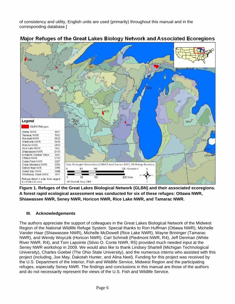
II. Goals, Objectives, and Participating Refuges We conducted a rapid ecological assessment of refuge-prioritized forest stands of six Laurentian Mixed Forest-Great Lakes Coastal Biological Network (hereafter, Great Lakes Biological Network) refuges: Ottawa National Wildlife Refuge (NWR), Shiawassee NWR, Seney NWR, Horicon NWR, Rice Lake NWR, and Tamarac NWR (Fig. 1, below). The goal of the rapid ecological assessment was to increase understanding of existing conditions of refuge forests and facilitate future monitoring and management. Objectives included the quantification of important compositional and structural patterns as they relate to the ecological integrity of forest stands. We also conducted on-site training so that refuge staff can collect more data in the future, and provided each refuge with a database of collected data and associated metrics (including plot photos) and an analysis of some composition and structural patterns. This manual provides detailed methodology used in the assessment, an equipment list, raw data sheets, and a list of metrics (and associated descriptions) that can be calculated based on field measurements. [For the sake

of consistency and utility, English units are used (primarily) throughout this manual and in the corresponding database.]

Figure 1. Refuges of the Great Lakes Biological Network (GLBN) and their associated ecoregions. A forest rapid ecological assessment was conducted for six of these refuges: Ottawa NWR, Shiawassee NWR, Seney NWR, Horicon NWR, Rice Lake NWR, and Tamarac NWR.

III. Acknowledgements

The authors appreciate the support of colleagues in the Great Lakes Biological Network of the Midwest Region of the National Wildlife Refuge System. Special thanks to Ron Huffman (Ottawa NWR), Michelle Vander Haar (Shiawassee NWR), Michelle McDowell (Rice Lake NWR), Wayne Brininger (Tamarac NWR), and Wendy Woyczik (Horicon NWR). Carl Schmidt (Piedmont NWR, R4), Jeff Denman (White River NWR, R4), and Tom Lapointe (Silvio O. Conte NWR, R5) provided much needed input at the Seney NWR workshop in 2009. We would also like to thank Lindsey Shartell (Michigan Technological University), Charles Goebel (The Ohio State University), and the numerous interns who assisted with this project (including, Joe May, Dakotah Hunter, and Alina Neel). Funding for this project was received by the U.S. Department of the Interior, Fish and Wildlife Service, Midwest Region and the participating refuges, especially Seney NWR. The findings and conclusions in this manual are those of the authors and do not necessarily represent the views of the U.S. Fish and Wildlife Service.

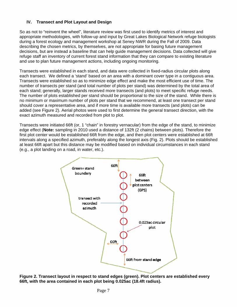
IV. Transect and Plot Layout and Design So as not to “reinvent the wheel”, literature review was first used to identify metrics of interest and appropriate methodologies, with follow-up and input by Great Lakes Biological Network refuge biologists during a forest ecology and management workshop at Seney NWR during the Fall of 2009. Data describing the chosen metrics, by themselves, are not appropriate for basing future management decisions, but are instead a baseline that can help guide management decisions. Data collected will give refuge staff an inventory of current forest stand information that they can compare to existing literature and use to plan future management actions, including ongoing monitoring. Transects were established in each stand, and data were collected in fixed-radius circular plots along each transect. We defined a ‘stand’ based on an area with a dominant cover type in a contiguous area. Transects were established so as to minimize edge effect and make the most efficient use of time. The number of transects per stand (and total number of plots per stand) was determined by the total area of each stand; generally, larger stands received more transects (and plots) to meet specific refuge needs. The number of plots established per stand should be proportional to the size of the stand. While there is no minimum or maximum number of plots per stand that we recommend, at least one transect per stand should cover a representative area, and if more time is available more transects (and plots) can be added (see Figure 2). Aerial photos were used to first determine the general transect direction, with the exact azimuth measured and recorded from plot to plot. Transects were initiated 66ft (or, 1 “chain” in forestry vernacular) from the edge of the stand, to minimize edge effect (Note: sampling in 2010 used a distance of 132ft (2 chains) between plots). Therefore the first plot center would be established 66ft from the edge, and then plot centers were established at 66ft intervals along a specified azimuth, preferably along the longest axis (Fig. 2). Plots should be established at least 66ft apart but this distance may be modified based on individual circumstances in each stand (e.g., a plot landing on a road, in water, etc.).

Figure 2. Transect layout in respect to stand edges (green). Plot centers are established every 66ft, with the area contained in each plot being 0.025ac (18.4ft radius).

The 0.025ac circular plots were used as a trade-off between sampling extensively and intensively to collect stand-level data. The radius of these plots was 18.4ft (Fig. 3). From the center of these plots, we then established three sub-plot transects for use in measuring coarse woody debris (CWD) and other variables: one sub-plot transect at 0 degrees, one sub-plot transect at 135 degrees and one sub-plot transect at 225 degrees. We used three pieces of rope to lay out the sub-plot transects, one piece had a mark at 3.3ft, one at 6.6 ft, and one at 13.1ft. The quadrats were placed at the mark on each piece of rope. The ropes were randomly assigned to an azimuth (0, 135 or 225) in each plot so that the quadrats were not always in the pattern shown in Figure 3 (e.g., the rope with the mark at 3.3ft did not always have to be on the 0 line, etc.).

Figure 3. Plot design, with coarse woody debris (CWD) and herbaceous cover sub-plot transects at 0, 135 and 225 degrees. One 1m2 (10.9ft2) quadrat is placed on each line, one at 3.3ft from center, one at 6.6ft, and one at 13.1ft.

V. Field Measurements The following field measurements were taken within each plot (in the order they appear on the data sheet, see Appendix IV). A brief description of the field measurement follows each. We used a new data sheet at the start of sampling each stand and recorded the stand name at the top of that data sheet, therefore a separate column for stand name or number was not necessary to include. Each participating Refuge may want to add variables to address specific interests, such as stand age, physiographic class, etc. 1. N Coord: GPS North Coordinate (decimal degrees, NAD83) 2. W Coord: GPS West Coordinate (decimal degrees, NAD83)

3. Plot.: Numbering starts with 1 (first plot from stand edge) and proceeds in order thereafter.

4. Pic: The photograph number corresponding to plot center of each plot, facing NORTH. 5. Densiometer (Dens N, E, S, W): Holding the spherical densiometer as required at each plot center,

four densiometer readings (percent closed canopy) are taken while facing N, E, S, and W. By averaging these four values, the vagaries of densitometer readings are reduced and this average value (with standard deviation) may be used in further analyses.

6. Tree: The tree number, in order, starting at north and recording and measuring trees clockwise within plot; only woody stems (i.e., trees) >5” diameter breast height (DBH) are measured. 7. Spp.: The tree species code (see Table 1 for species code). 8. DBH: (diameter at breast height measured for each tree >5” DBH)

9. Status: 1 = alive; 2 = dead 10. Class: The crown class for each tree recorded and measured (Class 1 = dominant, Class 2 = co- dominant, Class 3 = intermediate, Class 4 = suppressed, see Table 3 and Figure 4 for descriptions and diagrams for each crown class).

11. Vigor: The tree vigor code (see Table 3 for descriptions of each vigor rating). 12-17. Damage (Dam1, 2), location (Loc 1,2) & severity (Sev 1,2): Record up to two damages (see Tables 4-6 and Figures 6-33 for descriptions and diagrams for damage).

18-21. CWD (CWD0, 135, 225): Measure only pieces of CWD that are >5” diameter (at the largest end) and > 4’ length and that intersect one of the sub-plot transects. The wood must be >5” diameter

and below Decay Class 5 at the point of intersection with the transect. Diameter is measured by holding a tape above the log at a position perpendicular to the length, if the tape cannot be wrapped around the log. Measure both the small-end diameter (sm dia) and large-end diameter (lg dia) of the CWD pieces. Small-end diameter is measured at the end of the log (5” minimum). Large-end diameter is measured at the point that best represents the overall log volume. Identify CWD to tree species (by species code) if possible. Determine decay class (decay) (see Table 8 for descriptions and diagrams). Decay class of the log is recorded as the decay class of the piece of wood that intersects the transect. Record data in the column of the sub-plot transect that is intersected.

Data collected within quadrats along sub-plot transects: One 1m2 (10.9ft2) quadrat is placed on each line, one at 3.3ft from center, one at 6.6ft, and one at 13.1ft. 22. Quadrat: labeled 0, 135 or 225 corresponding to the transect degrees.

23-25. Percent cover of woody plants, herbaceous plants, and lichens/mosses are recorded in

each quadrat (see table 8 for rankings). Invasive species are also measured by % cover, and identified by species (see below). A Refuge may want to record the dominant species of woody or herbaceous cover if interested.

23. Woody%C: Percent cover of woody plants are recorded in each quadrat (T= trace, 1-25%,

26-50%, 51-75%, > 75%). 24. Herb%C: Percent cover herbaceous plants are recorded in each quadrat (T= trace, 1-25%,

26-50%, 51-75%, > 75%).

25. Moss%C: Percent cover of lichens & mosses are recorded in each quadrat (T= trace,

1-25%, 26-50%, 51-75%, > 75%).

26-29. Invasive Name & Invasive Cover (Inv Name1, Inv Cover1): Name and percent cover of invasive species are recorded in each quadrat (T= trace, 1-25%, 26-50%, 51-75%, > 75%) by species (% cover by species is recorded). Space for two invasive species is provided on data sheet, add more columns if necessary.

30-33. MidStory Name & Count (Mid1 Name, Mid1 Count): Midstory trees are counted within each quadrat. A midstory tree is > 4.5’ tall but < 5” DBH. This measures regeneration within a stand. Midstory trees are counted by species (FIA spp codes, see Table 1). Space for two midstory species is provided on data sheet, add more columns if necessary.

Table 1. Species codes for woody plants (list may not include all species found at all refuges). See: http://www.fia.fs.fed.us/library/field-guides-methods-proc/docs/core_ver_4-0_10_2007_p2.pdf Code Common Name Genus species 012 balsam fir Abies balsamea 094 white spruce Picea glauca 095 black spruce Picea mariana 105 jack pine Pinus banksiana 125 red pine Pinus resinosa 129 white pine Pinus strobus 130 scotch pine Pinus sylvestris 241 northern white-cedar Thuja occidentalis 261 eastern hemlock Tsuga canadensis 310 maple spp. Acer spp. 313 boxelder Acer negundo 314 black maple Acer nigrum 315 striped maple Acer pensylvanicum 316 red maple Acer rubrum 317 silver maple Acer saccharinum 318 sugar maple Acer saccharum 319 Norway maple Acer platanoides 356 serviceberry Amelanchier spp. 371 yellow birch Betula alleghaniensis 375 paper birch Betula papyrifera 391 American hornbeam Carpinus caroliniana 402 bitternut hickory Carya cordiformis 403 pignut hickory Carya glabra 405 shellbark hickory Carya laciniosa 407 shagbark hickory Carya ovata 452 Northern catalpa Catalpa speciosa 462 hackberry Celtis occidentalis 490 dogwood spp. Cornus spp. 491 flowering dogwood Cornus florida 500 hawthorn Crataegus spp. 531 American beech Fagus grandifolia 541 white ash Fraxinus americana 542 black ash Fraxinus nigra 544 red ash/green ash Fraxinus pennsylvanica 552 honeylocust Gleditsia triscanthos

480 mulberry Morus spp. 602 black walnut Juglans nigra 680 mulberry Morus alba 693 blackgum Nyssa sylvatica 701 hop-hornbeam Ostrya virginiana 740 aspen spp. Populus spp. 742 Eastern cottonwood Populus deltoides 743 bigtooth aspen Populus grandidentata 746 trembling aspen Populus tremuloides 760 cherry spp. Prunus spp. 762 black cherry Prunus serotina 800 oak (deciduous) Quercus spp. 802 white oak Quercus alba 804 swamp white oak Quercus bicolor 809 northern pin oak Quercus ellipsoidalis 823 bur oak Quercus macrocarpa 833 northern red oak Quercus rubra 837 black oak Quercus velutina 901 black locust Robinia pseudoacacia 920 willow spp. Salix spp. 931 sassafras Sassafras albidum 951 American basswood Tilia americana 972 American elm Ulmus americana 975 slippery elm Ulmus rubra 999 unknown Table 2. Crown classes. 1= Dominant – trees with crown extending above the general level of the crown canopy and receiving full light from above and partly from the sides. These trees are taller than the average trees in the stand and their crowns are well developed, but they could be somewhat crowded on the sides. Also, trees whose crowns have received full light from above and from all sides during early development and most of their life. Their crown form or shape appears to be free of influence from neighboring trees. 2= Co-dominant – trees with crowns at the general level of the crown canopy. Crowns receive full light from above but little direct sunlight penetrates their sides. Usually they have medium-sized crowns and are somewhat crowded from the sides. In stagnated stands, co-dominant trees have small-sized crowns and are crowded on the sides. 3= Intermediate – trees that are shorter than dominants and co-dominant. They receive little direct light from above and none from the sides. As a result, intermediate trees usually have small crowns and are very crowded from the sides. Intermediate trees may be short but as long as their bole is relatively straight, they will receive this designation. If the tree is crooked and has a lot of bends in the bole from trying to get light, it should be categorized as suppressed. 4= Suppressed -- trees with crowns entirely below the general level of the crown canopy that receive no direct sunlight either from above or the sides. Suppressed trees usually have multiple bends in the bole for the tree as the tree looks for light, and excessive side branching as well.

Figure 4. Examples of crown classes: 1= dominant, 2= co-dominant, 3= intermediate, 4= suppressed. Table 3. Tree vigor/condition codes and criteria. Code Criteria 1 Crown with relatively few dead twigs; foliage density and color normal;

occasional small dead branches in upper crown; occasional large branch stubs on upper bole

2 Crown with occasional large dead branch in upper portion; foliage density below normal; some small dead twigs at top of crown; occasional large branch stubs on upper bole

3 Crown with moderate dieback; several large dead branches in upper

crown; bare twigs beginning to show; several branch stubs on upper and mid bole

4 Approximately half of crown dead 5 Over half of crown dead 6 Tree dead; not cut, standing with fine twigs (less than 2.54 cm (1 in) in

diameter) attached to branches 7 Tree dead (natural death); not cut; standing without fine twigs but still has

some branches attached to bole of tree

8 Tree dead; standing but bole only, no branches attached to bole

2 3 4 2 4 3 2 3 4 1 2 4

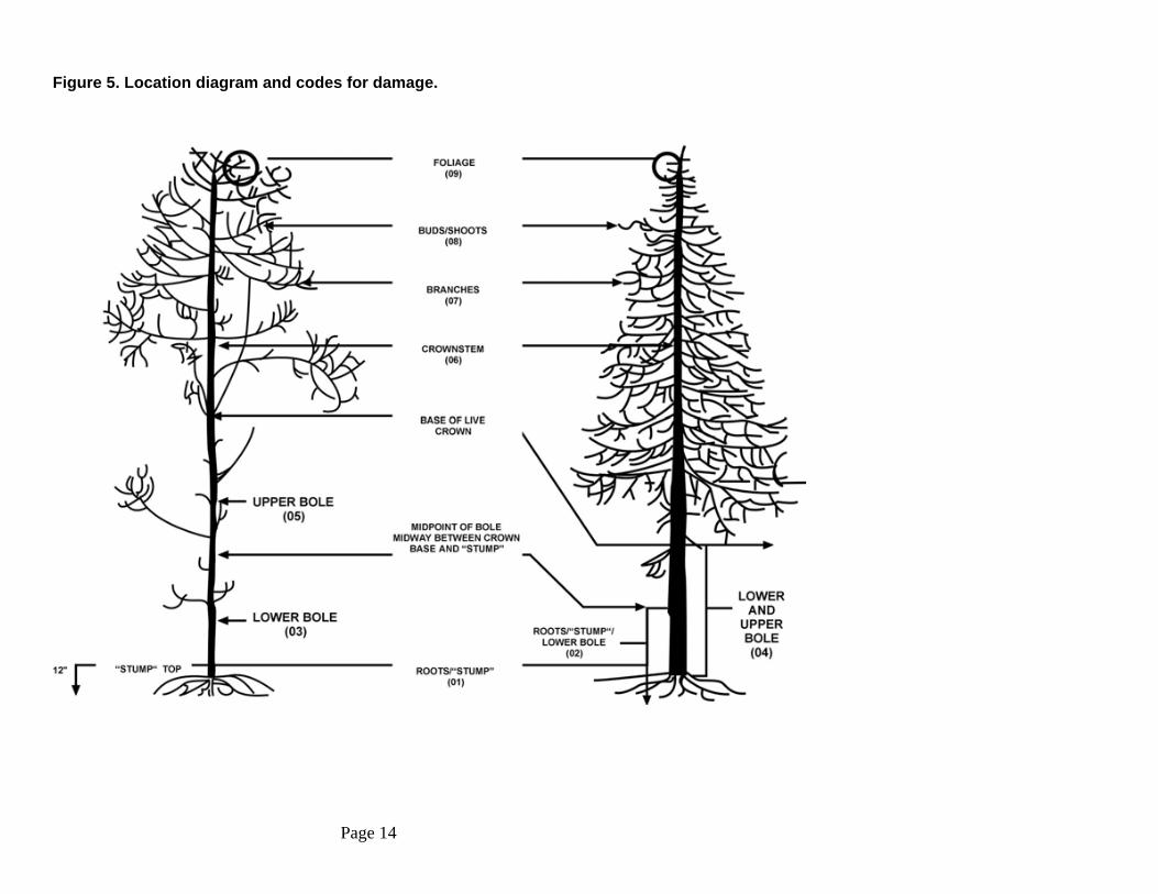
Table 4. Damage (location and damage type) codes. There is room to record up to two damages, the location, the type, and the severity. Record all damages following the same procedures outlined below. Look for damages starting from the base of the tree up. If the damage occurs in two or more locations, record the location in which the damage is most severe. If multiple damages occur in the same location, list the one that has the higher severity level. Record the first damage type observed that meets the damage threshold definition in the lowest location. Damage categories are recorded based on the numeric order that denotes decreasing significance from damage 01 - 31. Location codes are as listed below: 0 No damage. 1 Roots (exposed) and stump (12 inches in height from ground level). 2 Roots, stump, and lower bole. 3 Lower bole (lower half of the trunk between the stump and base of the live crown). 4 Lower and upper bole. 5 Upper bole (upper half of the trunk between stump and base of the live crown). 6 Crownstem (main stem within the live crown area, above the base of the live crown). 7 Branches (>1 in at the point of attachment to the main crown stem within the live crown area). 8 Buds and shoots (the most recent year’s growth). 9 Foliage. Damage type codes: 1 Canker, gall 2 Conks, fruiting bodies, and signs of advanced decay 3 Open wounds 4 Resinosis or gummosis 5 Cracks and seams (5 feet or longer) 11 Broken bole or roots (less than 3 feet from bole) 12 Brooms on roots or bole 13 Broken or dead roots (beyond 3 feet) 20 Vines in the crown 21 Loss of apical dominance, dead terminal 22 Broken or dead branches (at least 20% of tree) 23 Excessive branching or brooms within the live crown area 24 Damaged buds, foliage or shoots 25 Discoloration of foliage 31 Other

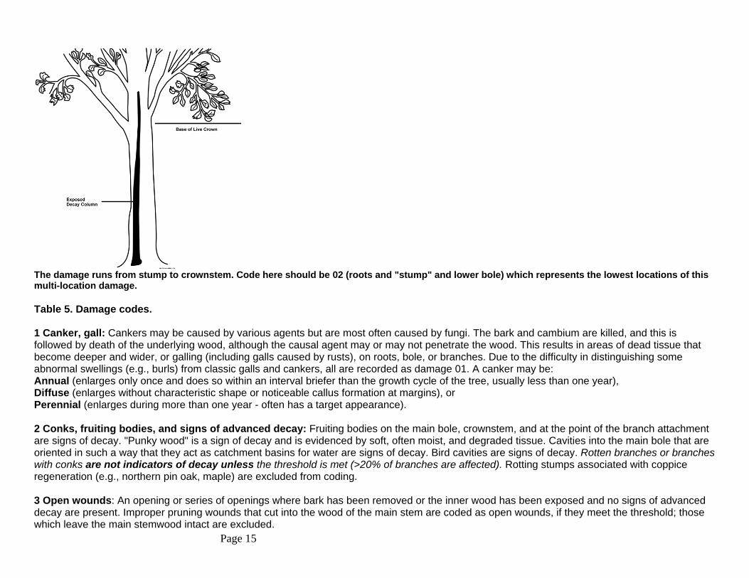
Figure 5. Location diagram and codes for damage.

The damage runs from stump to crownstem. Code here should be 02 (roots and "stump" and lower bole) which represents the lowest locations of this multi-location damage. Table 5. Damage codes. 1 Canker, gall: Cankers may be caused by various agents but are most often caused by fungi. The bark and cambium are killed, and this is followed by death of the underlying wood, although the causal agent may or may not penetrate the wood. This results in areas of dead tissue that become deeper and wider, or galling (including galls caused by rusts), on roots, bole, or branches. Due to the difficulty in distinguishing some abnormal swellings (e.g., burls) from classic galls and cankers, all are recorded as damage 01. A canker may be: Annual (enlarges only once and does so within an interval briefer than the growth cycle of the tree, usually less than one year), Diffuse (enlarges without characteristic shape or noticeable callus formation at margins), or Perennial (enlarges during more than one year - often has a target appearance). 2 Conks, fruiting bodies, and signs of advanced decay: Fruiting bodies on the main bole, crownstem, and at the point of the branch attachment are signs of decay. "Punky wood" is a sign of decay and is evidenced by soft, often moist, and degraded tissue. Cavities into the main bole that are oriented in such a way that they act as catchment basins for water are signs of decay. Bird cavities are signs of decay. Rotten branches or branches with conks are not indicators of decay unless the threshold is met (>20% of branches are affected). Rotting stumps associated with coppice regeneration (e.g., northern pin oak, maple) are excluded from coding. 3 Open wounds: An opening or series of openings where bark has been removed or the inner wood has been exposed and no signs of advanced decay are present. Improper pruning wounds that cut into the wood of the main stem are coded as open wounds, if they meet the threshold; those which leave the main stemwood intact are excluded.

4 Resinosis or gummosis: The origin of areas of resin or gum (sap) exudation on branches and trunks. 5 Cracks and seams: Cracks in trees are separations along the radial plane greater than or equal to 5ft. When they break out to the surface they often are called frost cracks. These cracks are not caused by frost or freezing temperature, though frost can be a major factor in their continued development. Cracks are most often caused by basal wounds or sprout stubs, and expand when temperatures drop rapidly. Seams develop as the tree attempts to seal the crack, although trees have no mechanism to compartmentalize this injury. Lightning strikes are recorded as cracks when they do not meet the threshold for open wounds. 11 Broken bole or roots (less than 3ft from bole): Broken roots within 3ft from bole either from excavation or rootsprung for any reason. Examples include those which have been excavated in a road cut or by animals. Stem broken in the bole area (below the base of the live crown) and tree is still alive. 12 Brooms on roots or bole: Clustering of foliage about a common point on the trunk. Examples include ash yellows witches' brooms on white and green ash and eastern and western conifers infected with dwarf mistletoes. 13 Broken or dead roots (beyond 3 feet): Roots beyond 3ft from bole that are broken or dead. 20 Vines in the crown: Kudzu, grapevine, ivy, dodder, etc. smothers tree crowns. Vines are rated as a percentage of tree crown affected. 21 Loss of apical dominance, dead terminal: Mortality of the terminal of the crownstem caused by frost, insect, pathogen, or other causes. 22 Broken or dead: Branches that are broken or dead. Branches with no twigs are ignored and not coded as dead. Dead or broken branches attached to the bole or crownstem outside the live crown area are not coded. 20% of the main, first order portion of a branch must be broken for a branch to be coded as such. For woodland species only: since dead branches often originate below the 12 in stump height and must be measured for DRC, there is no requirement that damage to branches can only occur to branches that originate within the live crown area. 23 Excessive branching or brooms within the live crown area: Brooms are a dense clustering of twigs or branches arising from a common point that occur within the live crown area. Includes abnormal clustering of vegetative structures and organs. This includes witches' brooms caused by ash yellows on green and white ash and those caused by dwarf mistletoes. 24 Damaged buds, foliage or shoots: Insect feeding, shredded or distorted foliage, buds or shoots >50% affected, on at least 30% of foliage, buds or shoots. Also includes herbicide or frost-damaged foliage, buds or shoots. 25 Discoloration of foliage: At least 30% of the foliage is more than 50% affected. Affected foliage must be more of some color other than green. If the observer is unsure if the color is green, it is considered green and not discolored. 31 Other: Use when no other explanation is appropriate. Specify in the tree notes section.

Table 6. Severity codes (by damage type). Damage Code 01—Canker, gall Measure the affected area from the outer edges of the canker or gall at any vertical section that is 3-ft and where at least 20% of circumference is affected. When looking at the tree 40% of the circumference is visible from any side, use this as a basis to determine the minimum 20% necessary. For location 1, the roots beyond 3ft must be affected. For location 7, at least 20% of branches must be affected. Record in 10% classes as shown below. See below for measuring diagram. Severity classes for code 01 (percent of circumference affected): Classes Code 20-29 2 30-39 3 40-49 4 50-59 5 60-69 6 70-79 7 80-89 8 90-99 9

A canker which exceeds threshold. Since 40% of circumference is visible from any side, and since over half the visible side is taken up by the canker, it obviously exceeds the 20% minimum circumference threshold. Damage Code 02 -- Conks, fruiting bodies, and signs of advanced decay Severity classes for code 02: None. Enter code 0 regardless of severity, except for roots > 3ft from the bole, or number of branches affected - 20%

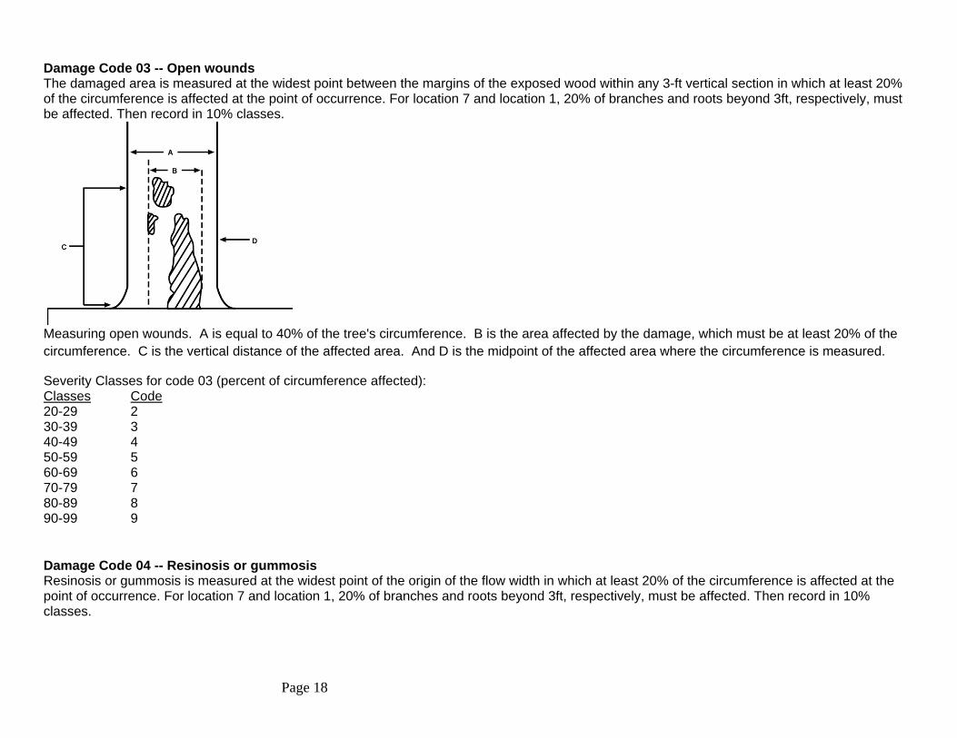
Damage Code 03 -- Open wounds The damaged area is measured at the widest point between the margins of the exposed wood within any 3-ft vertical section in which at least 20% of the circumference is affected at the point of occurrence. For location 7 and location 1, 20% of branches and roots beyond 3ft, respectively, must be affected. Then record in 10% classes.

Measuring open wounds. A is equal to 40% of the tree's circumference. B is the area affected by the damage, which must be at least 20% of the circumference. C is the vertical distance of the affected area. And D is the midpoint of the affected area where the circumference is measured.

Severity Classes for code 03 (percent of circumference affected): Classes Code 20-29 2 30-39 3 40-49 4 50-59 5 60-69 6 70-79 7 80-89 8 90-99 9 Damage Code 04 -- Resinosis or gummosis Resinosis or gummosis is measured at the widest point of the origin of the flow width in which at least 20% of the circumference is affected at the point of occurrence. For location 7 and location 1, 20% of branches and roots beyond 3ft, respectively, must be affected. Then record in 10% classes.

Severity classes for code 04 (percent of circumference affected): Classes Code 20-29 2 30-39 3 40-49 4 50-59 5 60-69 6 70-79 7 80-89 8 90-99 9 Damage Code 05 -- Cracks and seams greater than or equal to 5 feet Severity class for code 05 -- Record "0" for the lowest location in which the crack occurs. For location 7 and location 1, 20% of branches and roots beyond 3ft, respectively, must be affected. Then record in 10% classes. Damage Code 11 -- Broken bole or roots less than 3ft from bole Severity classes for code 11: None. Enter code 0 regardless of severity. Damage Code 12 -- Brooms on roots or bole Severity classes for code 12: None. Enter code 0 regardless of severity. Damage Code 13 -- Broken or dead roots At least 20% of roots beyond 3ft from bole are broken or dead. Severity classes for code 13 (percent of roots affected): Classes Code 20-29 2 30-39 3 40-49 4 50-59 5 60-69 6 70-79 7 80-89 8 90-99 9 Damage Code 20 -- Vines in crown Severity classes (percent of live crown affected): Classes Code

20-29 2 30-39 3 40-49 4 50-59 5 60-69 6 70-79 7 80-89 8 90-99 9 Damage Code 21 -- Loss of apical dominance, dead terminal Any occurrence (> 1%) is recorded in 10% classes as a percent of the crownstem affected. Use trees of the same species and general DBH/DRC class in the area or look for the detached portion of the crownstem on the ground to aid in estimating percent affected. If a lateral branch has assumed the leader and is above where the previous terminal was, then no damage is recorded. Classes Code 01-09 0 10-19 1 20-29 2 30-39 3 40-49 4 50-59 5 60-69 6 70-79 7 80-89 8 90-99 9 Damage Code 22 -- Broken or dead branches At least 20% of branches are broken or dead. Classes Code 20-29 2 30-39 3 40-49 4 50-59 5 60-69 6 70-79 7 80-89 8 90-99 9

Damage Code 23 -- Excessive branching or brooms At least 20% of the crownstem or branches are affected. Classes Code 20-29 2 30-39 3 40-49 4 50-59 5 60-69 6 70-79 7 80-89 8 90-99 9 Damage Code 24 - Damaged buds, shoots or foliage At least 30% of the buds, shoots or foliage are chewed or distorted by more than 50% affected. Classes Code 30-39 3 40-49 4 50-59 5 60-69 6 70-79 7 80-89 8 90-99 9 Damage Code 25 - Discoloration of Foliage At least 30% of the foliage is more than 50% affected. Classes Code 30-39 3 40-49 4 50-59 5 60-69 6 70-79 7 80-89 8 90-99 9 Damage Code 31 -- Other Enter code 0 regardless of severity. Describe condition.

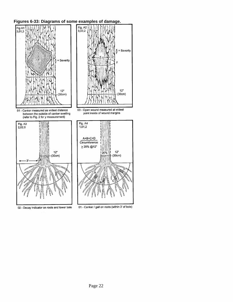
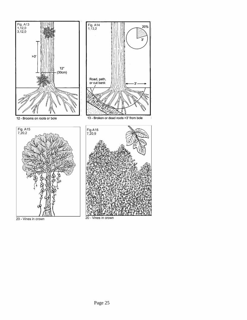
Figures 6-33: Diagrams of some examples of damage.

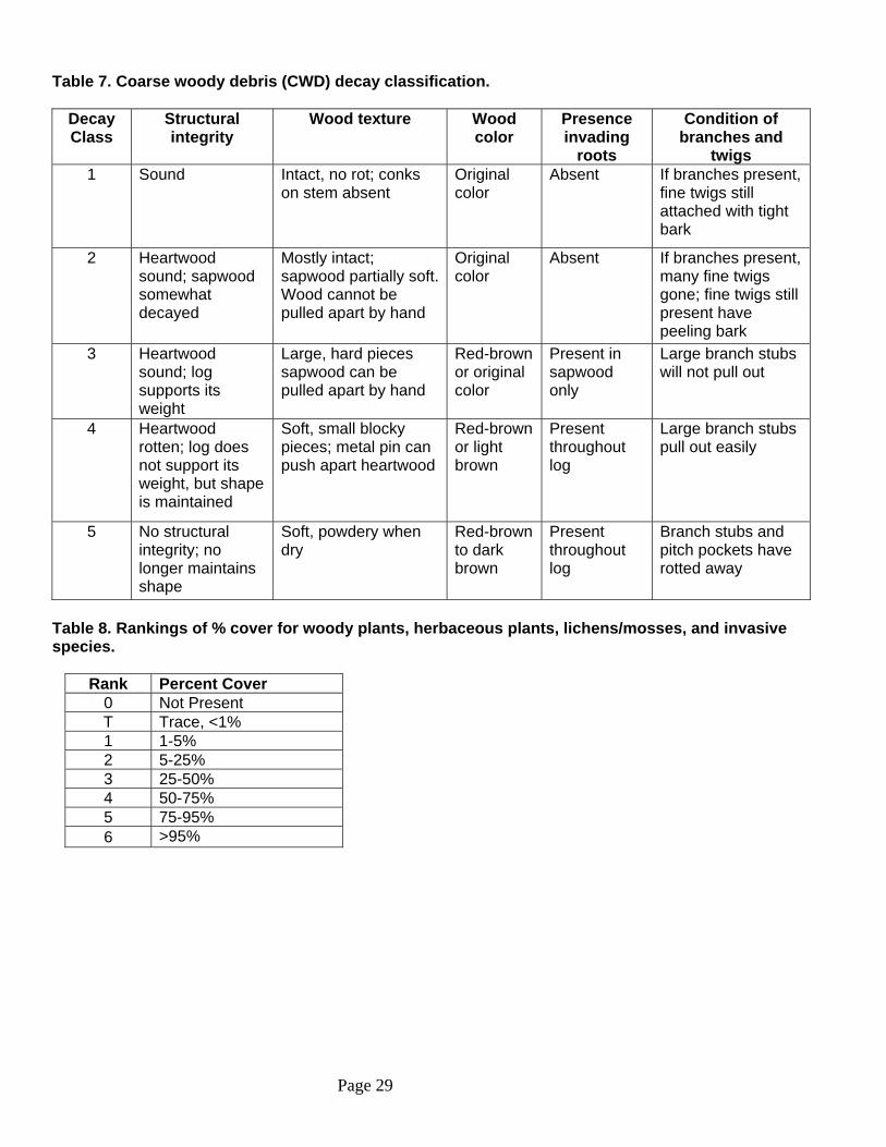
Table 7. Coarse woody debris (CWD) decay classification.

Decay Class

Structural integrity

Wood texture Wood color

Presence invading

roots

Condition of branches and

twigs 1 Sound Intact, no rot; conks

on stem absent Original color

Absent If branches present, fine twigs still attached with tight bark

2 Heartwood sound; sapwood somewhat decayed

Mostly intact; sapwood partially soft. Wood cannot be pulled apart by hand

Original color

Absent If branches present, many fine twigs gone; fine twigs still present have peeling bark

3 Heartwood sound; log supports its weight

Large, hard pieces sapwood can be pulled apart by hand

Red-brown or original color

Present in sapwood only

Large branch stubs will not pull out

4 Heartwood rotten; log does not support its weight, but shape is maintained

Soft, small blocky pieces; metal pin can push apart heartwood

Red-brown or light brown

Present throughout log

Large branch stubs pull out easily

5 No structural integrity; no longer maintains shape

Soft, powdery when dry

Red-brown to dark brown

Present throughout log

Branch stubs and pitch pockets have rotted away

Table 8. Rankings of % cover for woody plants, herbaceous plants, lichens/mosses, and invasive species.

Rank Percent Cover 0 Not Present T Trace, <1% 1 1-5% 2 5-25% 3 25-50% 4 50-75% 5 75-95% 6 >95%

VI. Appendices Appendix I. References. Barnes, B.V., D.R. Zak, S.R. Denton and S.H. Spurr. 1998. Forest ecology. John Wiley and Sons, New York. Corace, R.G. III, L.M. Shartell, L.A. Schulte, W.L. Brininger, Jr., M.K.D. McDowell and D.M. Kashian. 2011 (In

Press). An ecoregional context to forest management for National Wildlife Refuges of the Laurentian Mixed Forest Province. Journal of Environmental Management.

Forman, R.T.T. 1995. Land mosaics: the ecology of landscapes and regions. Cambridge University Press,

Cambridge. Franklin, J.E., H.H. Shugart and M.E. Harmon. 1987. Tree death as an ecological process. BioScience 37:550-

556. Franklin, J.F., T.A. Spies, R. Van Pelta, A.B. Carey, D.A. Thornburgh, D. Rae Berge, D.B. Lindenmayer, M.E.

Harmon, W.S. Keeton, D.C. Shaw, K. Bible and J. Chen. 2002. Disturbances and structural development of natural forest ecosystems with silvicultural implications, using Douglas-fir forests as an example. Forest Ecology and Management 155:399-423.

Frehlich, L.E. 2002. Forest dynamics and disturbance regimes. Cambridge University Press, Cambridge. Frehlich, L.E., M.W. Cornett and M.A. White. 2005. Controls and reference conditions in forestry: the role of

old-growth and retrospective studies. Journal of Forestry 103:339-344. Hagan, J.M. and A.A. Whitman. 2006. Biodiversity indicators for sustainable forestry: simplifying complexity.

Journal of Forestry 104:203-210. Hunter, M.L., Jr. 1990. Wildlife, forests, and forestry. Prentice-Hall, Inc., Englewood Cliffs, California. Johnson, S.E., E.L. Mudrak and D.M. Waller. 2006. A comparison of sampling methodologies for long-term

monitoring of forest vegetation in the Great Lakes Network National Parks. Great Lakes Network Report GLKN/2006/03, Ashland, Wisconsin. http://www.botany.wisc.edu/waller/publicationspdfs/Johnson_etal2006_NPSvegMonitoringReport.pdf

Lindenmayer, D.B., C.R. Margules and D.B. Botkin. 2000. Indicators of biodiversity for ecologically sustainable

forest management. Conservation Biology 14:941-950. Meffe, G.K., L.A. Nielsen, R.L. Knight and D.A. Schenborn. 2002. Ecosystem management. Island Press,

Washington. Meretsky, V.J., R.L. Fischman, J.R. Karr, D.A. Ashe, J.M. Scott, R.F. Noss and R.L.Schroeder. 2006. New

directions in conservation for the National Wildlife Refuge System. BioScience 56:135-143. Patton, D.R. 2011. Forest wildlife ecology and habitat management. CRC Press, Taylor and Francis Group,

Florida. Reams, G.A., W.D. Smith, M.H. Hansen, W.A. Bechtold, F.A. Roesch and G.G. Moisen. 2005. The forest

inventory and analysis sampling frame. Gen. Tech. Rep. SRS-80. Asheville, NC: U.S. Department of Agriculture, Forest Service, Southern Research Station. 21-36.

Schroeder, R.L., J.I. Holler and J.P. Taylor. 2004. Managing National Wildlife Refuges for historic and non-historic conditions: determining the role of the refuge in the ecosystem. Natural Resources Journal 44:1185-1210.

Scott, J.M., T. Loveland, K. Gergely, J. Strittholt and N. Staus. 2004. National Wildlife Refuge System:

ecological context and integrity. Natural Resources Journal 44:1041-1066. Webster, C.R., M.A. Jenkins and S. Jose. 2006. Woody invaders and the challenges they pose to forest

ecosystems in the eastern United States. Journal of Forestry 104:366-374.

Appendix II. Equipment list. Pencils Data sheets (plain and write-in-the-rain paper) Field manual (for reference) Digital camera (for pictures of plot center) Densiometer DBH Tape 1m2 quadrat Plot center set-up (typically rebar with 3 ropes attached; rebar is placed at plot center and one rope is placed at 0, 135 and 225 degrees. Each rope also has one marking on it (one at 3.3ft from center, one at 6.6ft, and one at 13.1ft) where the quadrat is placed. Compass GPS Unit Pin to mark center (if planning to revisit these sites in future)

Appendix III. Sample data sheets. PAGE 1 (FRONT): Refuge______________________________ Azimuth from plot-to-plot_____________________________

1 2 3 4 5 6 7 8 9 10 11 12 13 14 15 16 17 18 19 20 21 N Coord

W Coord Plot Pic Tree Spp DBH Status Class Vigor Dam1 Loc1 Sev1 Dam2 Loc2 Sev2 CWD0 CWD135 CWD225

DensN spp

DensE sm dia

DensS lg dia DensW decay spp

sm dia lg dia

decay

*Dens N, E, S & W have to be added (written in) at the beginning of each plot; they cannot be typed in ahead of time since we don’t know how many trees will be in each plot, therefore we don’t know how many rows each plot will take up on the data sheet. This is the same with CWD; we don’t know how many pieces of CWD will be in each plot, so the spp, sm dia, etc will have to be added in each time there is CWD measured in each plot. PAGE 2 (BACK):

22 23 24 25 26 27 28 29 30 31 32 33

Quadrat Woody%C Herb%C Moss%C Inv Name1

Inv Cover1

Inv Name2

Inv Cover2

Mid1 Name

Mid1 Count

Mid2 Name

Mid2 Count

rapid ecological assessment of forests in the laurentian

Documents