r-trees have grown everywhere - delab

R-trees Have Grown Everywhere

YANNIS MANOLOPOULOS

ALEXANDROS NANOPOULOS

APOSTOLOS N. PAPADOPOULOS

Aristotle University of Thessaloniki, Greece

and

YANNIS THEODORIDIS

University of Piraeus, Greece

Spatial data management has been an active area of intensive research for more than two decades.In order to support spatial objects in a database system several issues should be taken into con-sideration such as: spatial data models, indexing mechanisms, efficient query processing, costmodels. One of the most influential access methods in the area is the R-tree structure proposedby Guttman in 1984 as an effective and efficient solution to index rectangular objects in VLSIdesign applications. Since then, several variations of the original structure have been proposedtowards: providing more efficient access, handling objects in high-dimensional spaces, supportingconcurrent accesses, supporting I/O and CPU parallelism, efficient bulk-loading. It seems thatdue to the modern demanding applications and after the academia has paved the way, recentlythe industry recognized the use and necessity of R-trees. The simplicity of the structure and itsresemblance to the B-tree, allowed developers to easily incorporate the structure into existingdatabase management systems in order to support spatial query processing. In this paper we pro-vide an extensive survey of the R-tree evolution, studying the applicability of the structure and itsvariations to efficient query processing, accurate proposed cost models, and implementation issueslike concurrency control and parallelism. Based on the observation that ‘space is everywhere’,we anticipate that we are in the beginning of the era of the ‘ubiquitous R-tree’ in an analogousmanner as B-trees were considered 25 years ago.

Categories and Subject Descriptors: E.1 [Data]: Data Structures—trees; H.2.2 [Database Man-agement]: Physical Design—access methods; H.2.4 [Database Management]: Systems—queryprocessing, concurrency, parallel databases

General Terms: Algorithms, Management

Additional Key Words and Phrases: spatial data management, spatial query processing, selectivityand cost estimation

Author’s address: Yannis Manolopoulos, Alexandros Nanopoulos, Apostolos N. Pa-padopoulos, Department of Informatics, Aristotle University, 54006 Thessaloniki, Greece,{manolopo,alex,apostol}@delab.csd.auth.grYannis Theodoridis, Department of Informatics, University of Piraeus, 18534 Piraeus, [email protected]

Permission to make digital/hard copy of all or part of this material without fee for personalor classroom use provided that the copies are not made or distributed for profit or commercialadvantage, the ACM copyright/server notice, the title of the publication, and its date appear, andnotice is given that copying is by permission of the ACM, Inc. To copy otherwise, to republish,to post on servers, or to redistribute to lists requires prior specific permission and/or a fee.c© 20YY ACM 0004-5411/20YY/0100-0001 $5.00

ACM Computing Surveys, Vol. V, No. N, Month 20YY, Pages 1–0??.

2 · Yannis Manolopoulos et al.

1. INTRODUCTION

The paper entitled ‘The ubiquitous B-tree’ by Comer was published in ACM Com-puting Surveys in 1979 [36]. Actually, the keyword ‘B-tree’ was standing as ageneric term for a whole family of variations, namely the B*-trees , the B+-treesand several other minor variants [78]. The title of the paper might seem provocativeat that time. However, it represented a big truth, which is still valid in our days,since all textbooks on databases or data structures devote a considerable numberof pages to explain definitions, characteristics and basic procedures for searches,inserts and deletes on B-trees. Moreover, B+-trees are not just a theoretical no-tion. On the contrary, for years they remain the de facto standard access method inall prototype and commercial relational systems for typical transaction processingapplications, although one could observe that some quite more elegant and efficientstructures have appeared in the literature.

While the 80s were the period of the wide acceptance of relational systems inthe market, at the same time it became apparent that the relational model wasnot adequate to host new emerging applications. To name a few of them: multi-media, CAD/CAM, geographical, medical and scientific applications are just someexamples, where the relational model had been proven to behave poorly. Thus, theobject-oriented model and the object-relational model were proposed in the sequel.One of the reasons for the shortcoming of the relational systems was their inabilityto handle the new kind of data with B-trees. More specifically, B-trees were de-signed to handle alphanumeric (i.e., one-dimensional) data, like integers, charactersand strings, where an ordering relation can be defined. A number of new B-treevariations have appeared in the literature to handle object-oriented data (see [17]for a comparative study). Mainly, these structures were aiming at hosting data ofobject hierarchies of data in a single structure. However, these efforts had limitedapplicability and could not cover the requirements of the so many new applicationareas.

In light of this evolution, entirely novel access methods were proposed, evaluated,compared and established. One of these structures, the R-tree, was proposed byGuttman in 1984 aiming at handling geometrical data, such as points, line segments,surfaces, volumes and hyper-volumes in high-dimensional spaces [57]. R-trees weretreated in the literature in much the same way as B-trees. In particular, manyimproving variations have been proposed for various instances and environments,several novel operations have been developed for them and new cost models havebeen suggested. It seems that due to the modern demanding applications andafter the academia has paved the way, recently the industry recognized the use andnecessity of R-trees. Thus, R-trees are adopted as an additional access method tohandle multidimensional data. Based on the observation that ‘space is everywhere’[153], we anticipate that we are in the beginning of the era of the ‘ubiquitous R-tree’in an analogous manner as B-trees were considered 25 years ago. Nowadays, spatialdatabases and geographical information systems have been established as a maturefield, spatiotemporal databases and manipulation of moving points and trajectoriesare being studied extensively, and finally image and multimedia databases ableto handle new kinds of data, such as images, voice, music, or video, are beingdesigned and developed. An application in all these cases should rely to R-trees asACM Computing Surveys, Vol. V, No. N, Month 20YY.

R-trees Have Grown Everywhere · 3

a necessary tool for data storage and retrieval.R-tree applications cover a wide spectrum, from spatial and temporal to image

and video (multimedia) databases. The initial application that motivated Guttmanto his pioneering research was VLSI design (i.e., how to efficiently answer whethera space is already covered by a chip or not). Of course, handling rectangles quicklyfound application in geographical and, in general, spatial data, including GIS (build-ings, rivers, cities etc.), image or video/audio retrieval systems (similarity of ob-jects either in original space or in high-dimensional feature space), time series andchronological databases (time intervals are just 1D objects), and so on. Therefore,we argue that R-trees are found everywhere.

This survey aims at summarizing the literature relevant to R-trees. The structureof the paper is as follows. In Section 2, we present the original R-tree structure andits variants. The number of the R-tree variants is quite large and, therefore, weexamine them in several subsections, having in mind the special characteristics ofthe assumed environment or application. In Section 3, query processing issues arepresented by focusing on new types of queries, such as topological, directional anddistance operators. Section 4 presents work on query optimization, including ana-lytical cost models and histogram-based optimization techniques. The next sectiondescribes implementation issues concerning R-trees, such as parallelism and concur-rency control, and summarizes what is known from the literature about prototypeand commercial systems that have implemented them. The last section concludesthe survey.

2. THE FAMILY TREE OF R-TREES

The survey by Gaede and Guenther [47] annotates a vast list of citations related tomultidimensional access methods and, in particular, refers to R-trees to a significantextent. In the present survey, we are further focusing in the family of R-trees byenlightening the similarities and differences, the advantages and disadvantages ofthe various variations in a more exhaustive manner. Since the numbers of variantsthat have appeared in the literature is large, we group them according to the specialcharacteristics of the assumed environment or application and examine the membersof each group in chronological order.

2.1 Dynamic Versions of R-trees

In this subsection, we present dynamic versions of the R-tree, where the objectsare inserted on a one-by-one basis, as opposed to the case where a special packingtechnique can be applied to insert an apriori known static set of objects into thestructure by optimizing the storage overhead and the retrieval performance. Thelatter case will be examined in the next subsection. In simple words, here we focusin the way that dynamic insertions and splits are performed in assorted R-treevariants.

2.1.1 The Original R-tree. Although, nowadays the original R-tree is being de-scribed in many standard textbooks and monographs on databases [88; 101; 146;147], we briefly recall its basic properties. R-trees are hierarchical data struc-tures based on B+-trees. They are used for the dynamic organization of a setof d-dimensional geometric objects representing them by the minimum bounding

ACM Computing Surveys, Vol. V, No. N, Month 20YY.


d-dimensional rectangles (for simplicity, MBRs in the sequel). Each node of theR-tree corresponds to the minimum MBR that bounds its children. The leaves ofthe tree contain pointers to the database objects, instead of pointers to childrennodes. The nodes are implemented as disk pages.

It must be noted that the MBRs that surround different nodes may be overlap-ping. Besides, an MBR can be included (in the geometrical sense) in many nodes,but can be associated to only one of them. This means that a spatial search mayvisit many nodes, before confirming the existence or not of a given MBR.

The rules obeyed by the R-tree are as follows. Leaves reside on the same level.Each leaf contains pairs of the form (R, O), such that R is the MBR that containsspatially object O. Every other node contains pairs of the form (R,P ), where P isa pointer to a child of the node and R is the MBR that contains spatially the MBRscontained in this child. Every node (with the possible exception of the root) of anR-tree of class (m,M) contains between m and M pairs, where m ≤ dM/2e. Theroot contains at least two pairs, if it is not a leaf. Figure 1 depicts some objects onthe left and the corresponding R-tree on the right. Data rectangles R1 through R9

are stored in leaf nodes, whereas MBRs Ra, Rb and Rc are hosted in intermediatenodes.

��

��

��

��

��

��

��

��

��

��

��

��

Fig. 1. An R-tree example.

Insertions of new objects are directed to leaf nodes. At each level, the node thatwill be least enlarged is chosen. Thus, finally the object is inserted in an existingleaf if there is adequate space, otherwise a split takes place. The minimization ofthe sum of the areas of the two resulting nodes being the driving criterion, Guttmanproposed three alternative algorithms to handle splits, which are of linear, quadraticand exponential complexity:

Linear. Choose two objects as seeds for the two nodes, where these objects areas furthest as possible. Then, consider each remaining object in a random orderand assign it to the node requiring the smaller enlargement of its respective MBR.

Quadratic. Choose two objects as seeds for the two nodes, where these objectsif put together create as much dead space as possible (dead space is the spacethat remains from the MBR if the areas of the two objects are ignored). Then,until there are no remaining objects, choose for insertion the object for which thedifference of dead space if assigned to each of the two nodes is maximized, andinsert it in the node that requires smaller enlargement of its respective MBR.ACM Computing Surveys, Vol. V, No. N, Month 20YY.


Exponential. All possible groupings are exhaustively tested and the best is chosenwith respect to the minimization of the MBR enlargement.

Guttman suggested using the quadratic algorithm as a good compromise to achievereasonable retrieval performance.

In all R-tree variants that have appeared in the literature, tree traversals for anykind of operations are executed in exactly the same way as in the original R-tree(see next section). Basically, the variations of R-trees differ in the way they performsplits during insertions by considering different minimization criteria instead of thesum of the areas of the two resulting nodes. Therefore, in the sequel, we presentand annotate them according to their chronological order of appearance.

2.1.2 The R+-tree. R+-trees were proposed as a structure that avoids visitingmultiple paths during point queries and, thus, the retrieval performance could beimproved [160; 152]. This is achieved by using the clipping technique. In simplewords, R+-trees do not allow overlapping of MBRS at the same tree level. In turn,to achieve this, inserted objects have to be divided in two or more MBRs, whichmeans that a specific object’s entries may be duplicated and redundantly storedin various nodes. Therefore, this redundancy works in the opposite direction ofdecreasing the retrieval performance in case of window queries. At the same time,another side effect of clipping is that during insertions, an MBR augmentation maylead to a series of update operations in a chain-reaction type. Also, under certaincircumstances, the structure may lead to a deadlock, as, for example, when a splithas to take place at a node with M+1 rectangles, where every rectangle encloses asmaller one. An R+-tree for the same dataset illustrated in Figure 1, is presentedin Figure 2.

��

��

��

��

��

��

��

��

��

��

��

��

��

��

��

Fig. 2. An R+-tree example.

2.1.3 The R∗-tree. Although proposed in 1990 [12], R∗-trees are still very wellreceived and widely accepted in the literature as a prevailing performance-wisestructure that is often used as a basis for performance comparisons. The R∗-treedoes not obey the limitation for the number of pairs per node and follows a sophis-ticated node split technique. More specifically, the technique of ‘forced reinsertion’is applied, according to which, when a node overflows, p entries are extracted andreinserted in the tree (p being a parameter, with 30% a suggested optimal value).Other novel features of R∗-trees is that it takes into account additional criteriaexcept the minimization of the sum of the areas of the produced MBRs. The ben-efit from involving these criteria will be made clear later, in Section 4, where the



performance of the R∗-tree will be analyzed. These criteria are the minimizationof the overlapping between MBRs at the same level, as well as the minimization ofthe perimeter of the produced MBRs. The benefits from considering these criteriawill be made clear in Section 4, where the R∗-tree performance will be analyzed.Conclusively, the R∗-tree insertion algorithm is quite improving in comparison tothat of the original R-tree and, thus, improves the latter structure considerable asfar as retrievals are concerned (up to 50%). Evidently, the insertion operation isnot for free as it is CPU demanding since it applies a plane-sweep algorithm.

2.1.4 Hilbert R-tree. The Hilbert R-tree is a hybrid structure based on R-treesand B+-trees [77]. Actually, it is a B+-tree with geometrical objects being char-acterized by the Hilbert value of their centroid. Thus, leaves and internal nodesare augmented by the largest Hilbert value of their contained objects or their de-scendants, respectively. For an insertion of a new object, at each level the Hilbertvalues of the alternative nodes are checked and the smallest one that is larger thanthe Hilbert value of the object under insertion is followed. In addition, anotherheuristic used in case of overflow by Hilbert R-trees is the redistribution of objectsin sibling nodes. In other words, in such a case up to s siblings are checked in orderto find available space and absorb the new object. A split takes place only if alls siblings are full and, thus, s+1 nodes are produced. This heuristic is similar tothat applied in B*-trees, where redistribution and 2-to-3 splits are performed dur-ing node overflows [78]. According to the authors’ experimentation, Hilbert R-treeswere proven to be the best dynamic version of R-trees as of the time of publication.However, this variant is vulnerable performance-wise to large objects.

2.1.5 Linear Node Splitting. Ang and Tan in [7] have proposed a linear algo-rithm to distribute the objects of an overflowing node in two sets. The primarycriterion of this algorithm is to distribute the objects between the two nodes asevenly as possible, whereas the second criterion is the minimization of the over-lapping between them. Finally, the third criterion is the minimization of the totalcoverage. Experiments using this algorithm have shown that it results in R-treeswith better characteristics and better performance for window queries in compari-son with the quadratic algorithm of the original R-tree.

2.1.6 Optimal Node Splitting. Garcia, Lopez and Leutenegger elaborated theoptimal exponential algorithm of Guttman and reached a new optimal polynomialalgorithm O(nd), where d is the space dimensionality [49]. In the same paper, theauthors give another insertion heuristic, which is called ‘sibling-shift’. In particular,the objects of an overflowing node are optimally separated in two sets. Then, oneset is stored in the specific node, whereas the other set is inserted in a siblingnode that will depict the minimum increase of an objective function (e.g., expectednumber of disk access). If the latter node can accommodate the specific set, thenthe algorithm terminates. Otherwise, in a recursive manner the latter node is split.Finally, the process terminates when either a sibling absorbs the insertion or thisis not possible, in which case a new node is created to store the pending set. Theauthors reported that the combined use of the optimal partitioning algorithm andthe sibling-shift policy improves the index quality (i.e., node utilization) and theretrieval performance in comparison to the Hilbert R-trees, at the cost of increasedACM Computing Surveys, Vol. V, No. N, Month 20YY.


insertion time.

2.1.7 Branch Grafting. More recently, in [150] an insertion heuristic is proposedto improve the shape of the R-tree so that the tree achieves a more elegant shape,with a smaller number of nodes and better storage utilization. In particular, whena node overflows, then its father content is checked whether a sibling node withoverlapping MBR could accommodate any of the objects of the node in question.This technique is called branch grafting and could be considered as an eager methodhandling overflows locally at a reasonable cost, whereas forced reinsertion could beviewed as a lazy approach with higher costs whenever applied. The comparisonregards only various storage utilization parameters and not query processing effi-ciency.

2.1.8 Compact R-trees. Huang et al. proposed ‘compact R-trees’, a dynamicR-tree version with optimal space overhead [68]. Among the M+1 entries of anoverflowing node during insertions, a set of M entries is selected to remain in thisnode, under the constraint that the resulting MBR is the minimum possible. Then,the remaining entry is inserted to a sibling that (i) has available space, and (ii) itsMBR is enlarged the minimum possible. Thus, a split takes place only if there isnot available space in any sibling. The heuristic is quite simple to implement, itresults in storage utilization in the area of 97-99% (as opposed to 70% of the originalR-tree) at no extra insertion overhead, whereas the window query performance issimilar to that of the original R-tree.

2.1.9 cR-trees. Lastly, Brakatsoulas et al. have altered the assumption that anoverflowing node has to necessarily be split in exactly two nodes [22]. In particular,they relied on the k-means clustering algorithm and assumed that an overflowingnode can be split up to k nodes (k ≥ 2 being a parameter). Their experimentationshowed that the resulting index quality, the retrieval performance and the insertiontime are significantly better that those of R-trees (assuming quadratic split) andsimilar to those of R∗-trees.

2.1.10 Deviating Variations. Finally, other interesting variants have been pro-posed, which, however, in some sense deviate drastically from the original idea ofR-trees. Among other efforts, we note the following works. The Sphere trees byOosterom use minimum bounding spheres instead of MBRs [113], whereas the Celltrees by Guenther use minimum bounding polygons designed to accommodate ar-bitrary shape objects [52]. The Cell tree is a clipping-based structure and, thus, avariant of Cell trees has been proposed to overcome the disadvantages of clipping.The latter variant uses ‘oversize shelves’, i.e., special nodes attached to internalones, which contain objects that normally should cause considerable splits [53; 54].Similarly to Cell trees, Jagadish and Schiwietz proposed independently the struc-ture of Polyhedral trees or P-trees, which use minimum bounding polygons insteadof MBRs [70; 148]. The X-tree by Berchtold et al. uses the notion of ‘supernodes’(i.e., nodes of greater size) to handle overflows and avoid splits [15]. The S-tree byAggrawal et al. relaxes the rule that the R-tree is a balanced structure and mayhave leaves at different tree levels [3]. However, S-trees are static structures in thesense that they demand the data to be known in advance. Another recent effort by



Ang and Tan is the Bitmap R-tree [8], where each node contains bitmap descrip-tions of the internal and external object regions except the MBRs of the objects.Thus, the extra space demand is paid off by savings in retrieval performance due tobetter tree pruning. The same trade-off holds for the RS-tree, which is proposed byPark at al. [133] and connects an R∗-tree with a signature tree with an one-to-onenode correspondence. Agarwal et al. [4] proposed the Box-tree, that is, a bounding-volume hierarchy that uses axis-aligned boxes as bounding volumes. They provideworst-case lower bounds on query complexity, showing that box-trees are close tooptimal, and they present algorithms to convert box-trees to R-trees, resulting inR-trees with (almost) optimal query complexity. Lee and Chung [89] developed theDR-tree, which is a main memory structure for multi-dimensional objects. Theycouple the R∗-tree with this structure to improve the spatial query performance.Finally, Bozanis et al. have partitioned the R-tree in a number of smaller R-trees[21], along the lines of the binomial queues that are an efficient variation of heaps.

2.2 Static Versions of R-trees

There are common applications that use static data. For instance, insertions anddeletions in census, cartographic and environmental databases are rare or even theyare not performed at all. For such applications, special attention should be paid inorder to construct an optimal structure with regards to some tree characteristics,such as storage overhead minimization, storage utilization maximization, minimiza-tion of overlap or cover between tree nodes, or combinations of the above. There-fore, it is anticipated that query processing performance will be improved. Thesemethods are well known in the literature as ‘packing’ or ‘bulk loading’. Thus, nextwe examine such methods that require the data to be known in advance.

2.2.1 The Packed R-tree. The first packing algorithm was proposed by Rous-sopoulos and Leifker in 1985, soon after the proposal of the original R-tree [141].This first effort basically suggests ordering the objects according to some spatialcriterion (e.g., according to ascending x-coordinate) and then grouping them inleaf pages. No experimental work is presented to compare the performance of thismethod to that of the original R-tree. However, based on this simple inspiration anumber of other efforts have been proposed later in the literature.

2.2.2 The Hilbert Packed R-tree. Kamel and Faloutsos proposed an elaboratedmethod to construct a static R-tree with 100% storage utilization [76]. In partic-ular, among other heuristics they proposed sorting the objects according to theHilbert value of their centroids and then build the tree in a bottom-up manner.Experiments showed that the latter method achieves significantly better perfor-mance than the original R-tree with quadratic split, the R∗-tree and the PackedR-tree by Roussopoulos and Leifker in point and window queries. Moreover, Kameland Faloutsos proposed a formula to estimate the average number of node access,which is independent of the details of the R-tree maintenance algorithms and canbe applied to any R-tree variant.

2.2.3 The STR R-tree. STR (Sort-Tile-Recursive) is a bulk-loading algorithmfor R-trees proposed by Leutenegger et al. in [91]. Let N be a number of rectanglesin two-dimensional space. The basic idea of the method is to tile the address spaceACM Computing Surveys, Vol. V, No. N, Month 20YY.


by using S vertical slices, so that each slice contains enough rectangles to createapproximately

√N/C nodes, where C is the R-tree node capacity. Initially, the

number of leaf nodes is determined, which is P = dN/Ce. Let S =√

P . Therectangles are sorted with respect to the x coordinate of the centroids, and S slicesare created. Each slice contains S ·C rectangles, which are consecutive in the sortedlist. In each slice, the objects are sorted by the y coordinate of the centroids andare packed into nodes (placing C objects in a node). The method is applied untilall R-tree levels are formulated. The STR method is easily applicable to high di-mensionalities. Experimental evaluation performed in [91] has demonstrated thatthe STR method is generally better than previously proposed bulk-loading meth-ods. However, in some cases the Hilbert packing approach performs marginallybetter. It has to be noticed that Garcia et al. [50] proposed an R-tree node re-structuring algorithm for post-optimizing existing R-trees and improving dynamicinsertions, which incurs an optimization cost equal to that of STR. The resultingR-tree outperforms dynamic R-tree versions, like the Hilbert R-tree, with only asmall additional cost during insertions. Moreover, an analytical model to predictthe number of disk accesses for buffer management is described by Leutenegger andLopez [90], which evaluates the quality of packing algorithms measured by queryperformance of the resulting tree.

2.2.4 Top-Down Greedy Split. Unlike the aforementioned packing algorithmsthat build the tree bottom-up, the top-down greedy-split (TGS) method [48] con-structs the R-tree in a top-down manner. TGS recursively applies a splitting processthat partitions a set of N rectangles into two subsets by applying an orthogonal cutto a selected axis. This process must satisfy the following conditions: 1) the valueof an objective function should be minimized, 2) one subset has a cardinality i·S forsome i so that the resulting subtrees are packed. The method is recursively appliedto both subsets. The objective function has the form f(r1, r2), where r1, r2 are theMBRs of the two subsets produced. The performance evaluation of the methodreported in [48] has demonstrated that the TGS approach is generally better thanpreviously proposed packing algorithms.

2.2.5 Small-Tree-Large-Tree and GBI. The previous packing algorithms buildan R-tree access method from a set of spatial objects. The small-tree-large-treemethod (STLT) [32] performs efficient bulk insertions into an existing R-tree struc-ture. Let R be a set of spatial objects indexed by an already existing R-tree andN a set of new objects that must be inserted. Instead of inserting the objects inthe R-tree one-by-one, the STLT method constructs a small R-tree for N and theninserts the small R-tree into the large R-tree. Obviously, the efficiency of the re-sulting index depends on the data distribution of the small R-tree. If the objects inN cover a large part of the data space, then using the STLT approach will result inincreasing overlap in the resulting index. Therefore, the method is best suited forskewed data distributions. STLT is extended in [34], where the Generalized R-treeBulk-Insertion Strategy (GBI) is proposed. GBI inserts new incoming data sets intoactive R-trees as follows: it first partitions the data sets into a set of clusters andoutliers, then it constructs a small R-tree for each cluster, finding suitable placesin the original R-tree to insert the newly created R-trees, and finally it bulk-inserts



the new R-trees and the outliers in the original R-tree.

2.2.6 Buffer R-tree. Arge et al. [11] proposed the Buffer R-tree (BR) for per-forming bulk update and queries. BR is based on the buffer tree lazy bufferingtechnique and exploits the available main memory. Analytical results in [11] showthe efficiency of BR, whereas experimental results illustrates its superiority over thethe other methods. BR requires smaller execution times to perform bulk updatesand produces a better quality index in terms of query performance. Moreover, BR(differently from other methods) allows for simultaneous batch updates and queries.

2.2.7 R-tree with low stabbing number. deBerg et al. [40] have proposed an R-tree construction algorithm from a given set of spatial objects (focus is on notvery high dimensionality), and they prove that the resulting R-tree has good querycomplexity for point and range queries with ranges of small width. Their analysisis based on the stabbing number, i.e., the number of rectangles containing a givenpoint. The produced bounds are optimal for certain special cases. Nevertheless, nocomparison is performed against other methods.

2.3 Spatiotemporal R-tree Variants

Spatiotemporal access methods (STAMs) provide the necessary tools to query spa-tiotemporal data. A large number of the proposed methods are based on the wellknown R-tree structure. In the sequel, we introduce a number of STAMs and queryprocessing techniques related to spatiotemporal applications, such as bitemporalspatial applications, trajectory monitoring, and moving objects. All the presentedmethods are based on the concept of the R-tree.

2.3.1 3D R-trees. The 3D R-tree, proposed in [168], considers time as an extradimension and represents 2D rectangles with time intervals as three-dimensionalboxes. This tree can be the original R-tree [57] or any of its (ephemeral) variants.

The 3D R-tree approach assumes that both ends of the interval [t1, t2) of eachrectangle are known and fixed. If the end time t2 is not known, this approach doesnot work well. For instance, assume that an object extends from some fixed timeuntil the current time, now (refer to [35] for a thorough discussion on the notion ofnow). One approach is to represent now by a time instance sufficiently far in thefuture. This leads to excessive boxes and consequent poor performance. Standardspatial access methods (SAMs), such as the R-tree and its variants, are not wellsuited to handle such ‘open’ and expanding objects. One special case where thisproblem can be overcome is when all movements are known a priori. This wouldcause only ‘closed’ objects to be entries of the R-tree.

The 3D R-tree was implemented and evaluated analytically and experimentally[168; 171], and it was compared with the alternative solution of maintaining a spa-tial index (e.g., a 2D R-tree) and a temporal index (e.g., a 1D R-tree or a segmenttree). Synthetic (uniform-like) datasets were used, and the retrieval costs for puretemporal (during, before), pure spatial (overlap, above), and spatiotemporal oper-ators (the four combinations) were measured. The results suggest that the unifiedscheme of a single 3D R-tree is obviously superior when spatiotemporal queries areposed, whereas for mixed workloads, the decision depends on the selectivity of theoperators.ACM Computing Surveys, Vol. V, No. N, Month 20YY.


2.3.2 The 2+3 R-tree. One possible solution to the problem of ‘open’ geometriesis to maintain a pair of two R-trees [108]:

—a 2D R-tree that stores two-dimensional entries that represent current (spatial)information about data, and

—a 3D R-tree that stores three-dimensional entries that represent past (spatiotem-poral) information; hence the name 2+3 R-tree.

The 2+3 R-tree approach is a variation of an original idea proposed in [86] in thecontext of bitemporal databases, and which was later generalized to accommodatemore general bitemporal data [19; 18].

As long as the end time t2 of an object interval is unknown, it is indexed by the(2D) front R-tree, keeping the start time t1 of its position along with its ID. Whent2 becomes known, then:

—the associated entry is migrated from the front R-tree to the (3D) back R-tree,and

—a new entry storing the updated current location is inserted into the front R-tree.

Should one know all object movements a priori, the front R-tree would not be usedat all, and the 2+3 R-tree reduces to the 3D R-tree presented earlier. It is alsoimportant to note that both trees may need to be searched, depending on the timeinstance related to the posed queries.

2.3.3 The Historical R-tree. Historical R-trees (HR-trees, for short) have beenproposed in [107], implemented and evaluated in [108] and improved recently in[163]. This STAM is based on the overlapping technique. In the HR-tree, concep-tually a new R-tree is created each time an update occurs. Obviously, it is notpractical to physically keep an entire R-tree for each update. Because an updateis localized, most of the indexed data and thus the index remain unchanged acrossan update. Consequently, an R-tree and its successor are likely to have many iden-tical nodes. The HR-tree exploits this and represents all R-trees only logically. Assuch, the HR-tree can be viewed as an acyclic graph, rather than as a collection ofindependent tree structures.

With the aid of an array pointing to the root of the underlying R-trees, one caneasily access the desired R-tree when performing a timeslice query. In fact, oncethe root node of the desired R-tree for the time instance specified in the queryis obtained, the query processing cost is the same as if all R-trees where keptphysically.

The concept of overlapping trees is simple to understand and implement. More-over, when the number of objects that change location in space is relatively small,this approach is space efficient. However, if the number of moving objects from onetime instance to another is large, this approach degenerates to independent treestructures, since no common paths are likely to be found.

2.3.4 The RST-tree. The RST-tree [144] is capable of indexing spatio-bitemporaldata with discretely changing spatial extents. In contrast to the indexing structuresdescribed previously, the RST-tree supports data that has two temporal dimensionsand two spatial dimensions. The valid time of data is the time(s)—past, present,or future—when the data is true in the modeled reality, while the transaction time



of data is the time(s) when the data was or is current in the database [71; 158].Data for which both valid and transaction time is captured is termed bitemporal.

2.3.5 The MV3R-tree. To overcome the shortcomings of the 3D R-tree and theHR-tree, Tao and Papadias [164] proposed the MV3R-tree, consisting of a multi-version R-tree and small auxiliary 3D R-tree built on the leaves of the former.Through extensive experimentation, the MV3R-tree turned out to be efficient inboth timestamp and interval queries with relatively small space requirements.

2.3.6 The Partially Persistent R-tree. Kollios et al. in [79] recently proposed thepartially-persistent R-tree (PPR-tree), actually a directed acyclic graph of nodeswith a number of root nodes, where each root is responsible for recording a subse-quent part of the ephemeral R-tree evolution. The disadvantage of both indexingtechniques is that space requirements become prohibitive for agile datasets.

2.3.7 The TB-tree. The TB-tree (Trajectory Bundle) [136] relaxes a fundamen-tal R-tree property, i.e., keeping neighboring entries together in a node, and strictlypreserves trajectories such that a leaf node only contains segments belonging to thesame trajectory. This is achieved by giving up on space discrimination. The TB-tree indexes past locations of objects and supports continuous changes.

2.3.8 The Time-Parameterized R-tree. The aforementioned access methods fo-cus on providing access paths to present or past values of objects. An access methodthat is based on the R-tree structure and provides access to present and future val-ues is the Time-Parameterized R-tree [145]. This method is based on the concept ofnon-static MBRs of leaf and internal nodes. In other words, the MBR of an objector a tree node is a function of time. It is assumed that the velocity vector of eachobject is known. Based on the last location of the object and its velocity vector,one can determine the current object position in space. One basic characteristic ofthe TPR-tree structure is that the covering MBRs of the internal nodes are rarelyminimum (although they are conservative). In a recent work [138] an efficient vari-ation of the TPR-tree has been proposed that eliminates some basic disadvantagesof the structure and shows better performance in query processing.

2.4 R-trees in OLAP, Data Warehouses and Data Mining

R-trees have not been used only for storing and processing spatial or spatiotemporaldata. Modifications to the R-tree structure have been also proposed in order tohandle queries in OLAP applications, Data Warehouses and Data Mining.

Variations for OLAP and Data Warehouses store summary information in in-ternal nodes, and therefore in many cases it is not necessary to search lower treelevels. Examples of such queries are window aggregate queries, where parts of thedataspace are requested that satisfy certain aggregate constraints. Nodes totallycontained by the query window do not have to be accessed. One of the first effortsin this context was the variant of Ra∗-tree, which has been proposed for efficientprocessing of window aggregate queries, where summarized data are stored in inter-nal nodes in addition to the MBR [74]. The same technique has been used in [123]in the case of spatial data warehouses. In [165] the aP-tree has been introduced inorder to process aggregate queries on planar point data. Finally, in [124] a combi-nation of aggregate R-trees and B-trees has been proposed for spatiotemporal dataACM Computing Surveys, Vol. V, No. N, Month 20YY.


warehouse indexing.Recently, R-trees have been also used in the context of Data Mining. In par-

ticular, Spatial Data Mining systems [58] include methods that gradually refinespatial predicates, based on indexes like the R-tree, to derive spatial patterns, e.g.,spatial association rules [80]. Nanopoulos et al. [109], based on the R-tree structureand the closest-pairs query, developed the C2P algorithm for efficient clustering,whereas [110] proposed a density biased sampling algorithm from R-trees, whichperforms effective pre-processing to clustering algorithms.

3. QUERY PROCESSING

The processing of spatial queries presents significant requirements, due to the largevolumes of spatial data and the complexity of both objects and queries [115] Ef-ficient processing of spatial queries capitalize on the proximity of the objects,achieved by the R-tree, so as to focus the searching on objects that satisfy thequeries.

Besides efficiency, one of the main reasons for the popularity of R-tree indexesstems from their versatility, since they can efficiently support many types of spatialoperators. The most common types of operators are: a) Topological (e.g., find allobjects that overlap or cover a given object), b) Directional (e.g., find all objectsthat lie north of a given object), c) Distance (e.g., find all objects that lie in less thana given distance from a given object). These operators comprise basic primitivesfor developing more complex ones in applications that are based on managementof spatial data, such as GIS, cartography and many others.

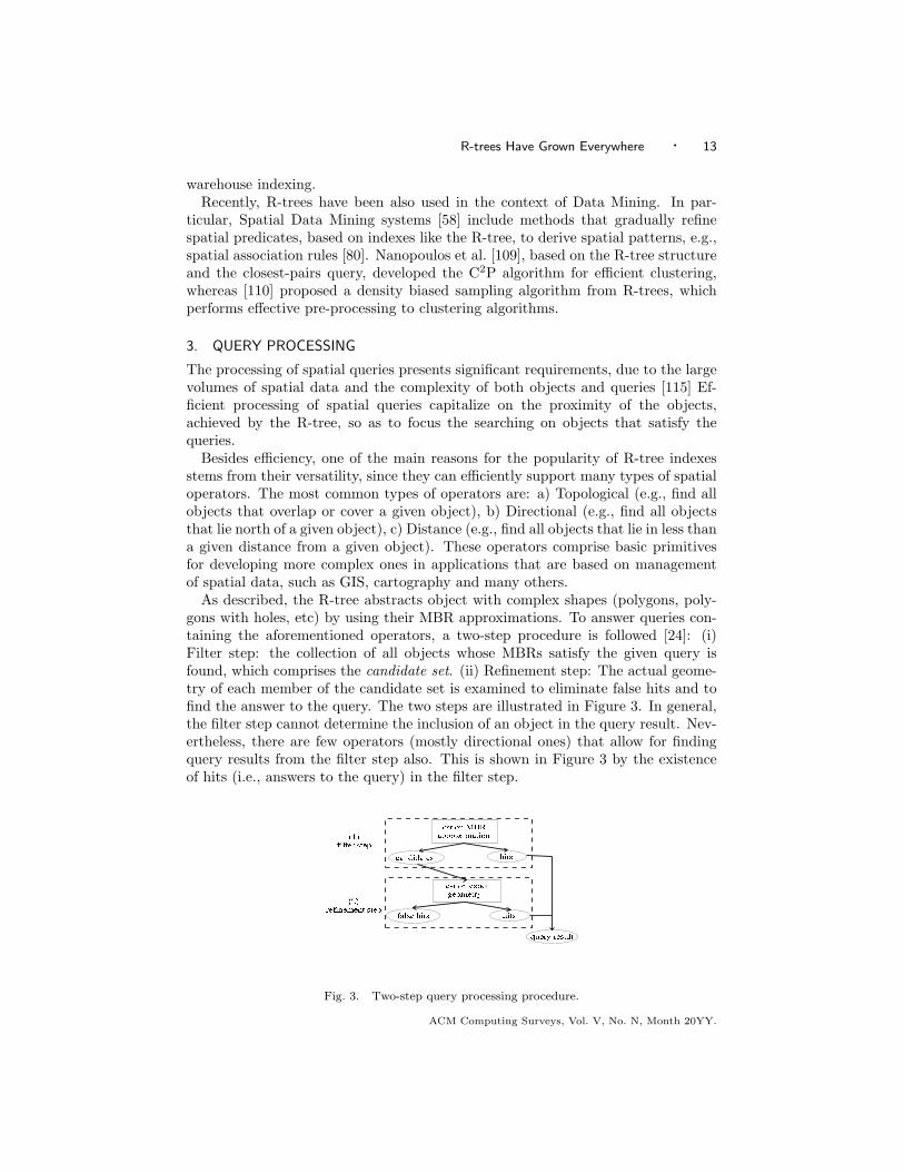
As described, the R-tree abstracts object with complex shapes (polygons, poly-gons with holes, etc) by using their MBR approximations. To answer queries con-taining the aforementioned operators, a two-step procedure is followed [24]: (i)Filter step: the collection of all objects whose MBRs satisfy the given query isfound, which comprises the candidate set. (ii) Refinement step: The actual geome-try of each member of the candidate set is examined to eliminate false hits and tofind the answer to the query. The two steps are illustrated in Figure 3. In general,the filter step cannot determine the inclusion of an object in the query result. Nev-ertheless, there are few operators (mostly directional ones) that allow for findingquery results from the filter step also. This is shown in Figure 3 by the existenceof hits (i.e., answers to the query) in the filter step.

��

��! #"%$�"��!&('�) *,+�-/.

0�132�465781:9,;=<>4? 1�5@A1>4CBED

FEG=H�IKJML,N�O/I P,QSR/T

UV#W!XZY[X\W�]�V,^�_

`�a!bc/dCe�f(g!hji�f(g!k

l(m�noqp=r/s�t#p>uAp>t�vxw�v�p!y

Fig. 3. Two-step query processing procedure.



In the following, we will describe in more detail the query processing techniquesthat have been developed for each query type. Since the refinement step is or-thogonal to the filtering step, the developed techniques have mainly focused on thelatter. More details on representations different from the MBR, and their impacton the refinement step can be found in [25].

3.1 Range and Topological Queries

The most common operation with an R-tree index is a range query, that is, thefinding of all objects that a query region intersects. In many cases the queryregion is a rectangle and the query is called window query. The processing of arange/window query is defined in [57]. It commences from the root node of thetree. For each entry whose MBR intersects the query region, the process descendsto the corresponding subtree. At the leaf level, for each object bounding rectanglethat intersects the query region, the corresponding object is examined (refinementstep). Also, it has to be mentioned that point queries (i.e., find all objects thatcontain a query point) can also be treated as a range query, since the query pointcan be considered as a degenerated rectangle. In [128] the case of combining theexecution of several range queries in order to achieve better overall performancewas considered.

The intersection operator, which is examined by the range query, can be consid-ered a special case of a more detailed retrieval of topological relations. Papadiaset al. [120] developed a systematic description of the topological information thatMBRs convey about the corresponding spatial objects, and proposed an algorithmto minimize the I/O cost of topological queries, that is, queries that involve topolog-ical relations. In particular, the intersection test of the range query corresponds tothe disjoint or non disjoint condition between the indexed objects (called primaryobjects, i.e., those contained in the R-tree) and the query object (called referenceobject). Although the disjoint relation is left unchanged, the non disjoint relationis refined further with the following relations: meet, equal, overlap, contains andcovers. Figure 4 depicts all possible relations between two objects.

� � � � � ��

�� ! #" $!%�&

Fig. 4. Topological relations: a) disjoint(q, p), b) meet(q, p), c) overlap(q, p), d) covers(q, p), e)contains(q, p) or inside(p, q), f) equal(q, p).

The topological relation between two MBRs does not necessarily coincide withthe topological relations between the two corresponding objects, because MBRsare approximate representations. Therefore, given two objects, the correspondingMBRs satisfy, in general, a number of possible relations [120]. In order to performa topological query with an R-tree, [120] defines the more general relations that willbe used for downwards propagation at the intermediate nodes. For convenience, wedenote the aforementioned approach as PTSE (from the names of the authors).ACM Computing Surveys, Vol. V, No. N, Month 20YY.


Experimental results in [120] indicate that the topological relations can be dividedin three categories, with respect to the incurred I/O cost. The first category con-tains relation disjoint, which requires the larger cost (almost equal to the scanningof the entire R-tree contents), the second contains relations meet, overlap, insideand covered by, which require medium cost, and the third the relations equal, cover,contains, which require small cost. Compared to the straightforward case where arange query is first executed and then the topological relations are examined onlyat the refinement step, the approach of [120] shows an improvement of up to 60%.

3.2 Directional Queries

R-trees have been also used to answer queries involving directional information (left,above, north etc.). Papadias et al. [119] discussed relations between points (e.g.north) and relations between non-point objects approximated by their MBRs (e.g.,strong-north, weak-north) and provided a methodology to support these types ofqueries when objects’ MBRs are indexed by an R-tree. The methodology includestwo steps:

(1) all node rectangles that could include hits are detected based on a directionrelation, possibly different from the target relation,

(2) the candidate hits are accessed based on another direction relation.

As in the case of topological queries, the above procedure that involves MBRsonly composes the filter step, while actual hits are detected during the refinementstep, which involves the exact geometry of objects. Consider the following example:assume we ask for objects p weak-north of an object q; each object p is approximatedby its MBR p′ and each rectangle r is defined by its lower-left corner rl and its upperright corner ru. The R-tree nodes P that might include hits are those that fulfillthe following constraint: Pu north of q′u and Pl south of q′u. Respectively, candidatehits p′ are those that fulfill the following constraint: p′u north of q′u and p′l northof q′l and p′l south of q′u. Following the same strategy, [119] supported a number ofdirectional queries and showed through experiments their performance.

3.3 Nearest Neighbor Queries

The problem of answering k nearest-neighbor (NN) queries using R-trees has beenintroduced by Roussopoulos et al. [142]. This approach is based on metrics thatmeasure the optimistic and pessimistic distances between the R-tree contents andthe query point1. Given a query point P and an object O that is represented by itsMBR, [142] describes two metrics. The first is called MINDIST and corresponds tothe minimum possible distance of P from O. The second is called MINMAXDISTand corresponds to the minimum of the maximum possible distances from P to avertex of O’s MBR. These two metrics comprise a lower and an upper bound onthe actual distance of O from P , respectively. More specifically, MINDIST(P, R)is the distance from P to the closest point on the boundary of R, which does notnecessarily have to be a corner point. MINMAXDIST(P,R) is the distance from Pto the closest corner of R that is adjacent (i.e., connected with an edge of R) to the

1The NN query can be also extended to non-point objects, by providing appropriate distancemeasures. See [63] for more details.



corner that is farthest from P . Figure 5 illustrates an example of the MINDISTand MINMAXDIST metrics between a two-dimensional query point P and threeMBRs (for the rectangle that includes P , MINDIST is equal to 0).

�

��

��

��

�� "!�#�$��&%�'

(*) +�(",�-�.�)&/�0

1*2 3�1�4�5�6�2&7�8

Fig. 5. Example of MINDIST and MINMAXDIST.

In [142], a branch-and-bound R-tree traversal algorithm is presented that usesthe aforementioned metrics to order and prune the search tree. The search or-dering determines the node visits during the tree traversal. As described in [142],MINDIST produces more optimistic ordering than MINMAXDIST, but there mayexist cases of data sets (depending on the sizes and the layouts of MBRs) wherethe latter produces less costly traversals. For a query point P , the pruning of nodevisits during the searching is performed according to the following heuristics. Thecomplete algorithm for finding the 1st NN is presented in Figure 6. 2

(1) An MBR M with MINDIST(P,M) greater than the MINMAXDIST(P,M ′) ofanother MBR M ′, is discarded because it cannot contain the NN. This is usedin downward pruning.

(2) An actual distance from P to a given object O, which is greater than theMINMAXDIST(P,M) for an MBR M , can be discarded because M containsan object O′ that is nearer to P . This is also used in downward pruning.

(3) Every MBR M with MINDIST(P, M) greater than the actual distance fromP to a given object O is discarded because it cannot enclose an object nearerthan O. This is used in upward pruning.

Cheung and Fu [33] have observed that a more efficient version of the aforemen-tioned branch-and-bound algorithm can be derived on the basis that pruning withrespect to the number of node accesses is considered. It is based on the observationthat only the third pruning heuristic is necessary to maintain the same number ofpruned nodes. (This observation was independently made also by [63].) However,this pruning heuristic has to be applied in a different position, thus resulting toa modified NN search algorithm, which we denote as MN. For these reasons, theNNSearch procedure of Figure 6 is modified by removing step 12 (which appliesthe first and second pruning heuristics) and by repositioning of step 3 (third prun-ing heuristic) before the recursive application of step 15. Thus, the for-loop ofsteps 13–17 is given in Figure 7.

2For finding k-NN (k > 1), the previous procedure can be easily modified so as to maintain thecurrent k most closest objects and by pruning with respect to the furthest object each time.



Procedure NNSearch(Node, Point, Nearest)1. if Node.type == LEAF2. for i=1 to Node.count3. dist = objectDIST(Point, Node.branch[i].rect)4. if dist < Nearest.dist5. Nearest.dist = dist6. Nearest.rect = Node.branch[i].rect7. endif8. endfor9. else10. genBranchList(branchList)11. sortBranchList(branchList)12. last = pruneBranchList(Node, Point, Nearest, branchList)13. for i = 1 to last14. newNode = Node.branch[branchList[i]]15. NNSearch(newNode, Point, Nearest)16. last = pruneBranchList(Node, Point, Nearest, branchList)17. endfor18. endif19. end

Fig. 6. Nearest Neighbor Search Algorithm.

13. for i = 1 to last14. Apply Pruning Heuristic 315. newNode = Node.branch[branchList[i]]16. NNSearch(newNode, Point, Nearest)17. endfor

Fig. 7. Modification in the NNSearch.

Finally, it has to be noticed that Belussi et al. [14] have proposed a nearest-neighbor algorithm for the R+-tree variant. Their method considers informationon the reference space to improve the search. The resulting data structure integratesthe R+-tree with a regular grid, indexed by using a hashing technique, combiningthe advantages of the rectangular space decomposition attained by R+-trees, witha direct access attained by hashing.

3.4 Incremental Nearest Neighbor Queries

Hjaltason and Samet [63] presented the problem of incremental NN searching withan R-tree. Incremental NN queries find the data objects in their order of distancefrom the query object (ranking). For instance, let a set of cities C and the query:‘find the nearest city to q ∈ C whose population is larger than 1 million people’. Byobtaining the neighbors incrementally, they can be examined against the specifiedcriterion. This operation is defined as distance browsing [63]. It has to be noticedthat it is different from searching for a prespecified k, because k cannot be knownin advance.



The algorithm for incremental NN searching is based on maintaining the set ofnodes to be visited in a priority queue (for the case of skewed and high-dimensionaldata, [63] proposes that the queue should be divided in several tiers, one of whichremains in main memory and the others on secondary storage). The entries in thequeue are sorted according to the MINDIST metric. It is assumed that the actualobjects (e.g., polygons) are stored separately in the data level, as long as eachobject is completely contained by its corresponding bounding rectangle. Thus, atthe leaf-level of the R-tree the object bounding rectangles (i.e., the MBRs of thedata objects) can advocate pruning. (In the following, the bounding rectangle ofan object O is denoted as [O].) The algorithm is depicted in Figure 8.

Procedure IncNNSearch(q)1. enqueue(PriorityQueue, root’s children)2. while PriorityQueue not empty3. element ← dequeue(PriorityQueue)4. if element is an object O or an object bounding rectangle [O]5. if element == [O] and not PriorityQueue empty

and objectDist(q, O) > First(PriorityQueue).key6. enqueue(PriorityQueue, O, objectDist(q, O)7. else8. Output element /*or if element is bounding rectangle, the associated object*/9. endif10. else if element is leaf node11. foreach object bounding rectangle [O] in element12. enqueue(PriorityQueue, [O], dist(q, [O])13. endfor14. else /*non-leaf node*/15. foreach entry e in element16. enqueue(PriorityQueue, e, dist(q, e)17. endfor18. endif19. endwhile20. end

Fig. 8. Optimal Nearest Neighbor Search Algorithm.

For the analysis of the incremental NN searching algorithm, [63] makes the keyobservation that any algorithm for the R-tree must visit all the nodes that intersectthe search region, and notices that the incremental algorithm visits exactly thesenodes. Based on the assumption of low dimensionality and uniform data distribu-tion, it is proven in [63] that the expected number of leaf node accesses for k-NNprocessing is O(k +

√k).

Evidently, the incremental NN search algorithm can be applied to the problemof finding the k NNs (for a specified k), since it can terminate after having foundthe first k neighbors. For this case, however, the approach of [63] differs from [142].The branch-and-bound algorithm of Section 3.3 traverses the index in a depth-firstfashion. Once a node is visited, its processing has to be completed even if other(sibling) nodes are more probable to contain the NN object; thus at each step onlyACM Computing Surveys, Vol. V, No. N, Month 20YY.


local decisions can be made [63]. In contrast, the described algorithm in [63] makesglobal decisions by using the priority queue to maintain the nodes that are going tobe visited, and chooses among the child nodes of all nodes that have been visited,instead of the current one. Thus, it uses a best-first traversal of the tree, and prunesthe visiting to nodes according to the third pruning heuristic. This approach hasthe characteristic of optimality with respect to the number of R-tree node visits,however not to the NN problem itself. (Interestingly enough, [16] have describedan analogous k-NN searching algorithm that is based on the approach of [61] (aprior version of [63]), which is called Optimal Nearest Neighbor Search.)

3.4.1 Comparison of Nearest Neighbor Algorithms. From the description of allthe k-NN algorithms (original branch-and-bound KNN [142], the modified MNN [33],and the incremental INN [63]) it follows that there are three design issues that affectthe performance of the NN searching:

(i) the criterion of ordering node visits,(ii) the manner of ordering node visits (i.e., traversal type), and(iii) the pruning heuristics.

Table I summarizes the selection made by each algorithm for the above issues,whereas the pruning heuristics are explained in Section 3.3.

KNN MNN INN

ordering MINDIST or MINMAXDIST MINDIST MINDIST

traversal type Depth-First Depth-First Best-First

pruning heuristics 1,2,3 3 3

Table I. Characterization of NN search algorithms.

Experimental results in [63] show that INN clearly outperforms KNN. Neverthe-less, it has to be noticed that the comparison for high-dimensional data is left asan open issue (where it has to be considered that the size of the priority queue mayincrease significantly and it has to be stored on disk).

3.5 Reverse and Conditional Nearest Neighbor Queries

3.5.1 Reverse Nearest Neighbors. Reverse NN queries find the set of databasepoints that have the query point as the NN. The reverse and the NN problems areasymmetric. If the NN of a query point q is a data point p, then it does not holdin general that q is the NN of p (i.e., q is not necessarily the reverse NN). Theaforementioned problem has been introduced in [83], however it was restricted tostatic data and specialized data structures. Stanoi et al. [159] have developed areverse NN algorithm for the R-tree, which can handle dynamic data efficiently.

The algorithm of [159] is based on the notion of space dividing lines. For thetwo-dimensional space, each point can be associated with three lines around it.They are denoted as l1, l2 and l3, where l1 is parallel to the x axis, and the anglebetween l1 and l2, l2 and l3, l3 and l1 is 2π/3. The left part of Figure 9 illustrates thearrangement of the three space dividing lines, which determine 6 regions (denotedas S1, . . . , S6).



According to [159], for a query point q and the corresponding region Si, eitherthe NN of q in Si is also the reverse NN, or there does not exist a reverse NN in Si.Therefore, for each of the Si regions, the NN of the query point has to be found.This set of points for all regions determine a candidate set that has to be examinedso as to identify the reverse NN. Hence, for the two-dimensional space, this limitsthe choice of RNN(q) to one or two points in each of the six regions [159]. Thecorresponding algorithm is depicted in the right part of Figure 9. (Note that thecomputations corresponding to all six regions is done in a single traversal and notseparately for each region).

��

� ��

��

��

��

� �

!#"

$�%

Procedure RNNSearch(Point)1. RNNResult = ∅2. CandidateList = CondNNSearch(q)3. EliminateDuplicates(CandidateList)4. foreach p ∈CandidateList5. NNSearch(p, r) /*r = NN(p)*/6. if objectDist(p, q) ≤ objectDist(p, r)7. RNNResult = RNNResult ∪ p8. endif9. endfor10. return RRNResult11. end

Fig. 9. Left: Space dividing lines. Right: Reverse Nearest Neighbor Search Algorithm.

3.5.2 Conditions Determined by Space Dividing Lines. Given one of the sixregions Si, the conditional NN determines the NN of the query point in Si. Thisprocedure is based on the observation that the examination of points that belongin MBRs that are out of Si, can be pruned. However, for an MBR that belongsto Si, their overlapping is done either fully or partially. This leads to five possiblecases for, e.g., the S2 region:

(1) MBR A: fully contained (all four vertices within S2).(2) MBR B: three vertices are in S2. Thus, there exist some data points in B that

are also contained in S2.(3) MBR C: two vertices are in S2. Thus, at least one data point of C is also in S2

(because an entire edge of C is in S2 and there exist at least one point on thatedge).

(4) MBR D: only one vertex is in S2. No implication can be done on the existenceof points in D that also belong in S2.

(5) MBR E: no vertices in S2, but part of E overlaps S2. No implication can bedone on the existence of points in D that also belong in S2, nor on the notexistence.

With the consideration of the aforementioned cases, the conditional NN searchingtraverses the tree and prunes out the sections that cannot lead to an answer eitherbecause a) their MBRs do not belong in the examined region, or b) because it canbe determined that other points in the region are closer to the query point.ACM Computing Surveys, Vol. V, No. N, Month 20YY.


3.5.3 Generalized Conditional Nearest Neighbor Searching. The conditional NNsearching that is determined by constraints due to space dividing lines is extendedby Ferhatosmanoglou et al. [46] to consider more general constraints. They definethe constrained NN (CNN) queries as NN queries that are constrained to a specifiedregion (determined by a convex polygon [46]). For instance, let a two-dimensionalmap, depicted in the left part of Figure 10, which contains several cities that arerepresented by points. Given the query point q, a CNN query is: find the nearestcity to the south of a q.3 Evidently, in unconditional NN search, the result wouldbe city a. In contrast, the result of the above CNN query is city b. Therefore, CNNqueries can combine directional and distance operators. Moreover, CNN queriescan involve multiple constraint regions [46].

A straightforward approach for the CNN problem (e.g., to first apply a rangequery with the specified constrained region and then search for the NNs in theresults of the range query, or to use INN [63] for finding nearest points in the orderof their distance and testing if they satisfy the given constraint at the same time)may unnecessarily retrieve a large number of points that do not belong in the queryregion, before finding the desired ones.

�

�

�

��

��

�� "!$#&%('*) ��+

,�-/.0,21�3�4�-65�798;:�<=,>< ?A@

B�C�D�E�C�F�G�H�I�J=BKJ=LAM

Fig. 10. Left: An example of CNN query. Right: The modified metrics for CNN.

For the above reasons, [46] proposes a new approach that merges the conditions ofNN and regional constraints in one phase. It is based on an extension of the workdescribed for the reverse NN, which considers general areas defined by polygonsinstead of the regions determined by space dividing lines. CNN again considers thefive possible cases for the overlap between the query region and an MBR, which weredescribed in Section 3.5.2. The MINDIST and MINMAXDIST metrics, however,are modified in a different way.

Let a query (i.e., constraint) region R, a query point q and an MBR M . Also,let the IR polygon be the intersection between R and M , i.e., IR = R∩M (severalwell known techniques exist to identify the intersection polygon). Then, havingcalculated the edges of IR polygon, [46] defines MINDIST(q, M, R) to be the min-imum of all distances from q to these edges. This case is illustrated in the rightpart of Figure 10, where it has to be noticed that MINDIST(q, M, R) offers atighter bound compared to MINDIST(q, M). Similarly, MINMAXDIST as definedby [142] does not hold when M is only partially contained in R. Therefore, [46]

3Although this constraint does not explicitly determine a convex polygon, as described in [46] thecombination of the directional line with the space boundary gives the desired polygon.



defines MINMAXDIST(q, M, R), which is computed only over the edges of M thatare completely contained in R (so as to identify the distance that guarantees theinclusion of a point from M in R). This case is illustrated in the right part ofFigure 10, where the shaded area represents IR, the original metrics are depictedwith dashed line and the modified ones with solid line.

3.6 Spatial Join Queries

Given two spatial relations A = {a1, . . . , an} and B = {b1, . . . , bm} (ai, bi arespatial objects), the spatial join computes all pairs (ai, bj), ai ∈ A, bj ∈ B thatsatisfy a spatial predicate, like the topological operators overlap (i.e., ai ∩ bj 6= ∅)and coverage (i.e., ai covers bj). For instance, such queries can find all rivers thatcross cities. Based on the two-step processing scheme (presented at the beginning ofSection 3), the R-tree facilitates the filter step, that is, the determination of all pairs(MBR(ai), MBR(bj)) that satisfy the required operator; for instance MBR(ai) ∩MBR(bj) 6= ∅, for the case of overlap. Spatial join queries, differently from selectionqueries (range and NN) that are single-scan, are characterized as multiple-scanqueries, since objects may have to be accessed more than once. Therefore, thesetypes of queries pose increased requirements for efficient query processing. In thefollowing, we examine the case of 2-way join, whereas the multi-way join is examinedin the next section.

3.6.1 Algorithm based on Depth-first Traversal. Brinkhoff et al. [23] first pre-sented an algorithm for the processing of spatial joins using R-trees. Let R and Sbe the joined R-trees. The basic form of the algorithm traverses the two R-trees ina depth-first manner, testing each time the entries of two nodes NR and NS , onefrom each tree respectively. Let ER ∈ NR and ES ∈ NS . If their MBRs do not in-tersect, then the further examination of the corresponding subtrees can be avoided.Otherwise, the algorithm proceeds recursively to the entries of the subtrees. Thispresents a search pruning criterion that capitalizes on the clustering properties ofthe R-tree. The description of the basic form of the algorithm is given in Figure 11.

Procedure RJ(NR, NS)1. foreach ES ∈ NS

2. foreach ER ∈ NR with MBR(ER) ∩ MBR(ES) 6= ∅3. if NR is leaf node /* NS is also a leaf */4. output(ER, ES)5. else6. RJ(ER.childPtr, ES .childPtr)7. endif8. endfor9. endfor10. end

Fig. 11. Basic Depth-First Spatial Join Algorithm.

In procedure RJ it is assumed (step 3) that both trees are of equal height. In [23]it is described that when the trees have different heights and the algorithm reachesACM Computing Surveys, Vol. V, No. N, Month 20YY.


a leaf node (whereas the other node is not a leaf), then window queries on thesubtrees rooted at the non-leaf node are performed with the MBRs of the entriesbelonging to the leaf node. Nevertheless, the experimental results in [23] indicatethat window queries do not profit very much from the proposed optimizations, thatwill described in the sequel; thus the performance of the join query may be impactedin this case. Also, to avoid as much as possible the multiple rereading of nodes, anLRU buffer is used.

In the basic form of the algorithm, each node entry is examined against all entriesof the other node. For this reason, two optimizations are proposed in [23]:

Restricting the search space: Let two nodes NR and NS , and I = MBR(NR) ∩MBR(NS) the intersection rectangle. This optimization is based on the obser-vation that only the entries ER ∈ NR and ES ∈ NS for which ER ∩ I 6= ∅ES ∩I 6= ∅ have to be examined, since they are the only that can have a commonintersection.

Spatial sorting and plane sweep: Given two nodes NR and NS , let Rseq and Sseq

represent the collection of the MBRs of the node entries. Rseq and Sseq are sortedwith respect to the lower-x coordinate values of their entries. The sequences areprocessed using a plane-sweep algorithm, where the sweep-line is moved each timeto the next unmarked rectangle among Rseq and Sseq with the smaller lower-x value, and the above procedure is repeated, until one of the two sequenceshas been exhausted. It has to be noted that the sorted node of entries is notmaintained in the nodes during insertions/deletions.

The reduction of I/O cost, compared to the basic form of the algorithm, isachieved in [23] with the computation of a read schedule, which controls the waythat nodes are fetched from the disk into the buffer. The following local optimiza-tion polices are proposed, which are based on spatial locality, and try to maintainin the buffer nodes whose MBRs are close in space:

Local plane-sweep order with pinning: It is based on the plane-sweep sequence,that was described for the tuning of CPU-time. Each time it pins in the bufferMBRs with the maximum number of intersections between it and the MBRs ofentries belonging to the other tree that have not been processed. Due to pinning,pages whose MBR frequently intersects other MBRs, are completely processedso as to avoid their rereading.

Local z-order: The intersections between the MBRs of the two nodes is first com-puted. Then, the MBRs are sorted with respect to a space filling curve, like thePeano curve, opting to bring together MBRs that are closed in space. As in theprevious case, the pinning of nodes is applied.

The overall experimental results (those that evaluate all the described optimiza-tions) indicate that the optimized form of the spatial join performs about 5 timesfaster than the basic one (notice that the basic form is CPU-bounded, whereas theoptimized is I/O-bounded).4

4It has to be noticed that [104] reported an improvement of the join execution time, by applyinga grid-based heuristic instead of plane-sweeping. However, no consideration was paid for the caseof buffer overflow.



3.6.2 Algorithm based on Breadth-first Traversal. Huang et al. [67], differentlyfrom the depth-first traversal of [23], propose the synchronous traversal of bothR-trees in a breadth-first manner, for the processing of spatial joins. This approachis based on the observation that the method of [23] does not have the ability toachieve a global optimization for the ordering of node visits, because the localoptimizations (read-scheduling) performed in [23] do not capture the access patternof nodes beyond the currently examined nodes. The BFRJ (Breadth-First R-treeJoin) algorithm of [67] opts for such global optimizations. The basic form of BFRJis depicted in Figure 12, where the results, i.e., pairs of intersected entries, at eachlevel l are maintained in the intermediate join index (IJIl) (when the two R-treesdo not have the same height, then when reaching the leaf level of one tree, BFRJwill have to proceed by descending the levels of the other tree, until the leaf-levelis reached also for this tree).

Procedure BFRJ(R, S)1. NR = root(R), NS = root(S)2. IJI0 = {(ER, ES) | ER ∈ NR, ES ∈ NS , MBR(ER) ∩MBR(ES) 6= ∅}3. for i=1 to height−− 14. foreach (ER, ES) ∈ IJIi5. NR = ER.childPtr, NS = ES .childPtr6. IJIi+1 = IJIi+1 ∪ {(E′R, E′S) | E′R ∈ NR, E′S ∈ NS , MBR(ER) ∩ MBR(ES) 6= ∅}7. endfor8. endfor9. output IJIi /* the IJI of leaf-level */10. end

Fig. 12. Breadth-First R-tree Join Algorithm.

Huang et al. [67] use the CPU-tuning optimizations proposed in [23], but proposethree new global optimizations for the tuning of I/O-time, which according to theexperimental results in [67] indicate an improvement in terms of disk accesses,compared to the approach of [23]. At level l, the global optimizations of BFRJ arebased on IJIl−1 to schedule the reading of nodes, and they are described as follows.

IJI Ordering: BFRJ orders the contents of IJI by trying not to spread too widelytheir multiple appearances. Since each member of IJI corresponds to two MBRs,this form of clustering may have to be performed concurrently for both of them.In [67] several options are considered for the processing, where the most efficient iswith respect to the sum of the centers (for each member of IJI, the x coordinatesof the centers of the two MBRs are calculated, and their sum is taken).

Memory Management of IJI: If not enough main memory exists, the contents of IJIhave to be stored on disk. BFRJ stores the contents only after the correspondinglevel has been completely written. However, with this option the shuffling of theIJI contents between disk and main memory cannot be avoided.

Buffer management of IJI: The multiple reading of nodes is further minimized byBFRJ by predicting which node will be fetched again in the sequel. Therefore,the buffer can purge nodes that have completed their processing.



For an easy comparison between the two described spatial join algorithms ([23;67]), Table II summarizes the options followed by each one.

[23] [67]

traversal type depth-first breadth-first

CPU-time restrict search space, plane-sweep restrict search space, plane-sweep

I/O-time plane-sweep/pinning, z-ordering IJI ordering, memoryand buffer management for IJI

Table II. Characterization of spatial join algorithms.

3.6.3 Join between an R-tree and a Non-index Data Set. In the case that anintermediate query result (e.g., of a range query) participates in the join, then anR-tree will not be available for it. A straightforward approach to perform the join inthis case is to apply multiple range queries, one for each object in the non-indexeddata set, over the R-tree of the other data set. Evidently, this approach is efficientonly when the size of the intermediate data set is very small.

An R-tree can be created (e.g., with bulk-loading) for the non-indexed data setin order to apply the already described algorithms for joining two R-trees [134].This approach, however, may introduce a non-negligible cost, required for the R-tree creation. In order to improve the latter approach, Lo and Ravishankhar [94]propose the use of the existing R-tree as a skeleton to build the seeded tree for thenon-indexed data set. Also, the sort-and-match algorithm [130] sorts the objectsof the non-indexed data set (using spatial ordering), creates leaf nodes that canbe accommodated in main memory, and examines each of them with leaves of theexisting R-tree of the other data set with respect to the join condition. An analo-gous approach is the Sort/Sweep Algorithm, developed in [56], which is based onplane sweeping. Arge et al. [10] propose the Priority Queue-Driven Traversal (PQ)algorithm, which combines the index-based and non-indexed based approaches suchthat in both forms can be processed using a single algorithm. Mamoulis and Papa-dias [98] propose the slot index spatial join (SISJ), which applies hash-join using thestructure of the existing R-tree to determine the extents of the spatial partitions.By additionally considering data that are indexed with quadtrees, [37] proposes analgorithm that joins a quadtree with an R-tree data structure. Moreover, Hoel andSamet [65] present a performance comparison of PMR quadtree join against joinfor several R-tree-like structures. All the aforementioned methods employ special-ized techniques to handle the non-index data set, which do not directly relate toquery processing for existing R-trees. The interested reader is directed to the givenreferences.

3.7 Multiway Spatial Join Queries

The spatial join algorithms that were examined in Section 3.6 focus on the caseof two R-trees. In GIS applications, large collections of spatial data may haveseveral thematic contents, thus they involve the join between multiple inputs. Mul-tiway spatial joins queries, proposed by Mamoulis and Papadias [100] (an earlierversion was presented in [121]), involve an arbitrary number of R-trees. Given n



data sets D1, . . . , Dn (each indexed with an R-tree) and a query Q, where Qij rep-resents the spatial predicate that should hold between Di and Dj , the multiwayjoin query finds all tuples {(r1,w, . . . , ri,x, . . . , rj,y, . . . rn,z) | ∀ i, j : ri,x ∈ Di, rj,y ∈Dj , ri,x Qij rj,y}. Therefore, multiway spatial join queries can be considered as ageneralization of pairwise spatial join that were presented in Section 3.6. QueryQ can be represented by a graph whose nodes correspond to the data sets Di andedges to join predicates Qij . In general, the query graph can be a tree (graphwithout cycles), a graph with cycles or a complete graph (every node connected toeach other). For instance, Figure 13 depicts these three different cases of a querygraph along with a tuple that satisfies the corresponding predicates (henceforth,based on [100], it is assumed for simplicity that each predicate Qij corresponds tothe spatial operator overlap).

��

��

��

��

� �"!�#

$ %

&'

( )

*+

,�-�.�-

/�01�2

3�4�5�67 8"9�:

; <

=>

?�@�A�@

B�CD�E

F�G�H�I

JLK"M�N

Fig. 13. Examples of multiway queries: a) Acyclic (chain) query. b) Query with cycle. c) Completegraph query.

One method to perform multiway spatial joins is the combination of a sequence ofpairwise joins (PJM). The order of pairwise joins is determined by the minimizationof expected I/O cost (in terms of page accesses). In this sequence, a pair doesnot necessarily correspond to a join between two R-trees (i.e., indexed data sets).Therefore, (i) RJ or BFRJ (see Section 3.6) is applied when both inputs are indexed,(ii) Slot Index Spatial Join (SISJ) [98] is applied when only one data set is indexed,and (iii) Hash spatial Join (HJ) [96] when none of the data sets is indexed (i.e.,they are intermediate results).

A different approach than PMJ is also described in [100; 121], called SynchronousTraversal (ST). ST starts from the root nodes and synchronously traverses theR-trees. It proceeds only with the combination of nodes that satisfy the querypredicates Qij , until reaching leaf nodes. ST is facilitated by the R-tree structureto decompose the problem into smaller local ones at each level. If fmax is themaximum node fanout, then in the worst case each local problem examines fn

max

combinations. The local problem is defined by:

—A set of n variables, v1, . . . , vn, each corresponding to an R-tree.—A domain Di, for each variable vi, which consists of the entries {Ei,1, . . . Ei,fi}

of node Ni in the Ri tree (fi is the fanout of Ni).—Each pair of variables (vi, vj) is constrained by predicate overlap, if Qij is true.

Based on [100], a binary assignment {vi ← Ei,x, vj ← Ej,y} is consistent iff(Qij is true) ⇒ (Ei,x overlaps Ej,y). A solution of a local problem is a n-tupleτ = (E1,w, . . . , Ei,x, . . . , Ej,y, . . . , En,z) such that ∀ i, j{vi ← Ei,x, vj ← Ej,y} isACM Computing Surveys, Vol. V, No. N, Month 20YY.


consistent. The objective of ST is the finding of all assignments of entries to vari-ables so as all predicates are satisfied.

Park et al. [131] made the observation that the optimization techniques of theoriginal 2-way R-tree join algorithm are still required in the case of multiway join,and they proposed the M-way join algorithm. Furthermore, Mamoulis and Papa-dias [100] propose two optimizations for the ST algorithm, which exploit the spatialstructure of the multiway join problem:

Static Variable Ordering (SVO): This heuristic pre-orders the problem variables byplacing the most constrained one first. Thus, variables are sorted in decreasingorder of their degree. SVO is applied once (before performing ST) and producesa static order that is used in find-combinations and space-restriction procedures.

Plane-Sweep combined with Forward Checking (PSFC): PSFC is an improved im-plementation of procedure find-combinations, which decomposes a local probleminto a series of smaller problems, one for each event of the sweep line. With thisheuristic, the overhead of searching and backtracking in large domains is avoided.

Experimental results in [100] show that the improvement due to SVO is significantwhen the few first variables are more constrained, whereas this does not applyfor complete query graphs. The combination of SVO-PSFC presents significantreduction in both I/O and CPU cost, compared to the version of ST that doesnot use these optimizations (PSFC performs better with increasing page size). Ingeneral, the savings in CPU cost are considered more significant in [100], since STis CPU bounded.

Finally, it has to be noticed that [100] proposes the optimization with dynamicprogramming to derive the query execution plan. Each time, either ST or PJMis selected for the intermediate executions. With this approach, execution plansthat are slightly more expensive (12% in the worst case) than the optimal one areselected [100]. Nevertheless, if n (the number of input R-trees) is larger than 10,the cost of the dynamic programming is prohibitive. For this reason, [100] alsodescribes a randomized search algorithm for finding the execution plan of largequeries, i.e., for large n.

3.8 Incremental Distance Join and Closest Pair Queries

3.8.1 Incremental Distance Join. Given two spatial relations A and B, distancejoin queries find the subset of the Cartesian product A×B, which satisfies an orderthat is based on distance. Halation and Samet [62] present an incremental approachfor processing distance join and distance semi-join queries (the latter is a variant ofthe former, and finds for each object in A the nearest object in B). The incrementalalgorithms for these queries that are described in [62] report the results one-by-one,with respect to the distance ordering. In contrast, the spatial join algorithms, thathave been described in Section 3.6, will first have to compute the entire result andthen to sort it before starting the output. Evidently, the focus of the incrementalalgorithm is on starting the output of results as early as possible.

For two R-trees R1 and R2, the Incremental Distance Join Algorithm (IDJ)maintains a set P of pairs (each pair has one item from R1 and R2 respectively).During the processing of P ’s entries, each time a pair p ∈ P is encountered thatcontains a node item n (i.e., not a data object), it is replaced by all pairs resulting by



substituting n with all its children nodes. The elements of P has to be maintainedsorted according to their distance. To achieve this, P is implemented as priorityqueue. The basic algorithmic form of IDJ is depicted in Figure 14, where theProcessNode procedure (which is also depicted) uses the same basic loop as theincremental NN algorithm of Section 3.4 (Item2 corresponds to the query object,for this reason the same notation [O] is used for the object bounding rectangles(OBRs)).

Procedure IDJ(R1, R2)1. Enqueue(Q, 0, (R1.root, R2.root))2. while Q not empty3. elem ← Q4. if both items of elem are data objects5. output elem /*elem = (O1, O2)*/6. else if both items OBRs7. D = objectDist(O1, O2)8. if Q empty or D ≤ Front(Q).dist9. output (O1, O2)10. else11. Enqueue(Q, D, (O1, O2))12. endif13. else if first item of elem is node14. ProcessNode(Q, elem, 1)15. else16. ProcessNode(Q, elem, 2)17. endif18. end

Procedure ProcessNode(Q, elem, order)/* elem = (i1, i2) */

1. if order == 12. Node = i1, Item2 = i13. else4. Node = i2, Item2 = i15. endif6. if Node is leaf7. foreach entry [O] of Node8. Enqueue(Q,dist([O],Item2,([O],Item2))9. endfor10. else11. foreach child c of Node12. Enqueue(Q, dist(c, Item2), (c, Item2))13. endfor14. endif15. end

Fig. 14. Basic form of Incremental Distance Join Algorithm.

In [62] optimizations are described over the basic form of the algorithm withrespect to the tie-braking criteria and the order of processing node items. Theevaluation of all described options is given in [62] through experimental results.These results indicate that the best performance is achieved by the combination ofthe following two optimizations: (i) Depth-first-like traversal: Elements containingdata objects or object bounding rectangles can be given priority over other elementswith the same distance (resolves tie-breaking); also, for elements containing non-leaf items, priority can be given to nodes at smaller level (i.e., deeper in the tree).(ii) Even: When a pair (n1, n2) with non-leaf nodes is retrieved from the head ofthe priority queue, the node at a higher level is chosen to be processed, to achievea more even traversal of the two trees (resolves the order of processing).

During the processing of the distance join, the priority queue may become verylarge. For the implementation of the priority queue [62] describes an approachthat is analogous to the one presented in Section 3.4, which divides the queue in anumber of partitions, where one is kept in main memory the others are maintainedon disk. Nevertheless, most of the pairs still will have a large distance and they willprobably never be retrieved by the queue. In order to limit the number of entriesACM Computing Surveys, Vol. V, No. N, Month 20YY.


in the priority queue, [62] proposes the use of restrictions based on a minimum anda maximum specified distance that the query results have to satisfy. If no suchconstraints on the distance can be posed by the user, [62] sets an upper bound onthe number of examined pairs (facilitated by the ‘STOP AFTER’ clause of SQL,which reports only a specified number K of results). This is done by estimatinga lower bound for the distance Dmax, which can be used to impose the requiredconstraint.

It has to be noticed that recently a k-distance join algorithm has been proposedby Shin et al. [157], which differently from [62], joins the first k pairs with re-spect to their distance. Their approach is based on a bi-directional expansion ofR-tree nodes and on plane-sweeping for pruning distant pairs. Moreover, they de-velop adaptive, multi-stage algorithms for k-distance join and incremental distancejoin algorithms. Experimental results illustrate the performance gains due to theadaptive algorithms over previous approaches (including [62]).

3.8.2 Distance Semi-Join. As mentioned, the distance semi-join query is a spe-cial case of the distance join query, since for each pair (o1, o2) in the result, theobject o1 appears only once (i.e., it does not appear in any other pair). In order toachieve this, [62] uses a set S0 to keep track of all first objects in each pair that isoutput.

The experimental evaluation in [62] indicates that the GlobalAll option presentsthe best performance. The GlobalAll option operates as follows: for each node anddata object in the first R-tree, the smallest dmax distance that has been encoun-tered so far, is maintained. A new pair (i1, i2) is enqueued only in the case thatits distance is smaller than dmax for i1. Since this option may require significantmemory space, dmax can be maintained for nodes only. Compared to the straight-forward approach of applying multiple NN queries (one for each object of the firstR-tree), the results of [62] show that the incremental algorithm outperforms thestraightforward one by up to 40%.

3.8.3 Finding Closest Pairs. As described, the incremental distance join algo-rithm can be easily modified to produce up to K pairs [62]. In this case, thealgorithm finds the K closest pairs between the two data sets, that is, the pairs ofobjects from the two data sets that have the K smallest distances between them(K=1 yields to the classic closest-pair problem of computational geometry). Forinstance, given a collection of archaeological sites and holiday resorts, the K closestpair query finds sites that have the K smallest distances to a resort, so as touriststo be accommodated easily.

Corral et al. [38] proposed a different approach, called CP, for closest pair queriesthan the one of [62]. Two types of algorithms have been investigated in [38], alsodescribed briefly in the sequel. (We present the case for K=1, since the extensionto K > 1 is easy, according to [38]. Also, we assume that the trees have the sameheight.)

Recursive based on sorting distances. This algorithm, called STD, descends the twoR-trees and keeps track of the closest distance T found so far. When two internalnodes are accessed, the MINMAXDIST is calculated for all pairs formed by theircontents. T can be updated (a kind of downward pruning) if it is larger than one



of such distances. When reaching the two leaf leaves, the actual object distancesare calculated and T is updated.5

Non-recursive based on heap Similar to [62], this algorithm, called HEAP, main-tains the pairs to be examined within a heap structure, sorted with respect toMINDIST metric. However, differently from [62], HEAP considers only pairsthat have MINDIST smaller than T . Moreover, similar to STD, HEAP updatesT with respect to the MINMAXDIST metric.

STD is a type of depth-first closest pair algorithm, which considers local opti-mizations. In contrast, HEAP and the incremental distance join algorithm belongto the type of best-first algorithms, which consider global optimizations. Also,recall that these two different algorithmic types have also been described for NNand join queries. Evidently, closest pair queries combine the characteristics of boththese types of queries. Regarding the tie-braking criteria, [38] describes severalones, however the best performance is achieved by resolving ties by giving priorityto the pair whose elements have the largest MBR. Also, if different tree heightsare addressed with two methods, then [38] proposes the Fix-at-root policy, whichstops the downwards propagation in the tree with lower level and continues thepropagation in the other tree, until a pair of nodes at the same level is found.

The comparison between STD and HEAP, which is experimentally performedin [38], indicates that HEAP outperforms STD for very small buffer sizes andfor data sets with large overlapping. For medium and large buffer sizes, STDclearly compares favorably to HEAP. Finally, in [39] the impact of buffering onthe performance of CP queries using R-trees was considered for several searchingapproaches and buffer replacement policies.

3.9 Classification of R-tree Query Processing Algorithms

In this section, we give a summary and a classification of all the described methods.The classification is given in Figure 15 and uses the same notation for the names ofthe algorithms as the one used throughout the previous sections. The links betweenthe contents of Figure 15 represent the relationships among them.

��

��

� �!� "$#!#

%�&'& (�)!) *,+!+

-�. /�02143 5�6 798': ;�<

=2>@?

ACBEDGF�H�HJILKMH�FONQPRF2SUT�H�VWVYX[Z'\^]_H�DG`!SUa'V

bdcfe�g�h

i�j�k�lnm�o�jqpsr�mnt�u

v�w�x

Fig. 15. Classification of the described R-tree based query processing methods.

5Note that STD is formed by a number of optimizations, which are presented separately in [38].Herein we only present STD in its final form because it significantly outperforms the others [38].



Four general types of spatial queries were presented, namely range, topological,NN and join queries. The algorithm for the range query (denoted as Gutt) is thefirst searching algorithm that was developed for the R-tree. Topological queries(the corresponding algorithm is denoted as PTSE) form a second type of queries,since they generalize the non-disjoint operator used by the range query. NN queriesinclude KNN and its improved version MNN, which address the finding of the k-NN.Moreover, based on KNN, RNN determines the reverse NNs. A different approachis followed by INN, which incrementally finds the NNs in the order of their distancefrom the query object. By generalizing the constraints of RNN, and based on INN(in order to achieve its ‘optimality’), CNN determines the NNs according to a queryconstraint. Therefore, constrained NN queries is a combination of range and NNqueries. Finally, the spatial join query between two R-trees is addressed by RJ(depth-first) and BFRJ (breadth-first). For the multiway join, PJM is based on RJin order to perform multiple pairwise joins, whereas ST traverses all trees at thesame time. IDJ (analogously to INN) focuses on the distance join (i.e., operatorwithin) and finds the results incrementally, in the order of the distance betweenthem. Closest pair queries (CP algorithm) find the k closest pairs between twoindexed data sets, and can be considered as combination of both NN and joinqueries. Finally, IDJ can also lead to the finding of closest pairs; for this reasonthere is a connection between CP and IDJ.

4. QUERY OPTIMIZATION ISSUES

Determining the best execution plan for a spatial query requires tools for measuring(more precisely, estimating) the number of (spatial) data items that are retrievedby a query as well as its cost, in terms of I/O and CPU effort. As in traditionalquery optimization, such tools include cost-based optimization models, exploitinganalytical formulae for selectivity (the hit percentage) and cost of a query, andhistogram-based techniques.

In particular for spatial databases supported by R-tree indices, cost-based opti-mization exploits analytical models and formulae that predict the number of hitsamong the entries of the R-tree and the cost of a query retrieval, measured in R-treenode accesses (or actual disk accesses, assuming existence of a buffering scheme).

Traditionally, R-tree performance has been evaluated by the ability to answerrange queries by accessing the smallest possible number of pages (i.e., nodes) inthe disk. Other queries, such as NN [142] and join queries [23] are also of greatinterest for a spatial query optimizer. Thus, Sections 4.1 and 4.2 survey work oncost models for selection and join queries, respectively, followed by Section 4.3,which presents sampling and histogram-based techniques.

4.1 Cost Models for Selection Queries

Considering that each R-tree node corresponds to a physical page in the disk, thecost estimation of a query (i.e., how many pages are accessed in order to retrievethe result of the query) turns into the problem of estimating the number of nodesvisited during R-tree traversal. Apparently, the actual time required (number ofdisk pages times the time required to read a page resident in disk) could be lessthan the estimated due to buffering. Therefore, several models have included bufferparameters in their formulae.



4.1.1 Formulae for Range Queries. The first attempt to estimate the perfor-mance of R-trees for range queries was made by Faloutsos et al. [44]. In thatpaper, the authors made two fundamental assumptions: (i) uniform distributionof data, and (ii) all the R-tree nodes were supposed to be full of data. For pointqueries, the cost formula derived expressed the fact that the number of nodes to bevisited equals the overlap of parent nodes per level or, in other words, the densityof nodes per level summed up for all but the leaf level (the authors did not use theterm density in that paper; this was used later in [167] as will be discussed below).

Although the analysis in [44] was restricted by the uniformity assumption andpacked trees, it served as a framework for almost all related work that appearedlater. Among the proposed formulae, one of the most useful was about the expectedheight h of an R-tree:

h = logfN

C(1)

where f is the fanout of parent nodes, C is the capacity of leaf nodes, and N is thenumber of data entries.

Later, Kamel and Faloutsos [76] and Pagel et al. [116] independently extendedthe analysis in [44] and presented the following formula that gives the averagecost CW of a range query with respect to a query window q = (q1, ..., qd), assum-ing the dataset is indexed by a d-dimensional R-tree and provided that the sides(sj , 1, ..., sj , d) of each R-tree node sj are known (the summation extends over alltree nodes).

CW (R, q) =∑

j

{d∏

i=1

(sj,i + qi)

}(2)

Eq. (2) allows the query optimizer to estimate the cost of a query window (mea-sured in number of node accesses) assumed that the corresponding R-tree has beenalready built and, hence, the MBR of each node sj of the R-tree can be measured.This formula, implicitly presents the dependency between the sizes of the R-treenodes and the query window, on the one hand, and the cost of a range query, on theother hand. Moreover, the influence of the node perimeters is revealed, which helpsunderstanding the R∗-tree efficiency as, it was the first method among the R-treevariants to take into account the node perimeter during its construction phase (seeSection 2.1 for relevant discussion and [166] for a performance-wise comparison ofthe most popular members of the R-tree family until that time).

Extending the work performed in [116], Pagel et al. in [117] proposed an optimalalgorithm that established a lower bound result for the performance of packed R-trees. It was also shown through experimental results that the best known static anddynamic R-tree variants, the packed R-tree by Kamel and Faloutsos [76] and the R∗-tree [12], respectively, performed about 10%-20% worse than the lower bound. [117]defined the problem of measuring the performance of SAMs like R-trees, as follows:For a bucket set B and a query model QM , let Prob(q meets Bi) be the probabilitythat performing query q forces an access of bucket Bi. Then the expected numberof bucket accesses needed to evaluate query q is called the performance measureACM Computing Surveys, Vol. V, No. N, Month 20YY.


PM for QM and is given by:

PM(QM, B) =m∑

i=1

Prob(q meets Bi) (3)

[117] also formalized the so called Bucket Set Problem (BSP): Given a set ofgeometric objects, a bucket capacity Cb ≥ 2, and a query model QM , determinethe bucket set Bopt for which the performance measure PM is minimal. Theyalso distinguished two cases, the simple case (called, SBSP) where Cb=2, and theuniversal case (called, UBSP) where Cb ≥ 3, and proved that SBSP can be solved inpolynomial time, while UBSP is NP-hard. Practically, this means that in R-treesetc. (where Cb = M >> 2), it is not possible to find and integrate an optimalconstruction algorithm.

The impact of the three parameters that are involved in Eq. (2), namely thearea sum of rectangles, the perimeter sum, and the number of rectangles, wasfurther studied in [118], where formulae for various kinds of range queries, suchas intersection, containment and enclosure queries of various shapes (points, lines,circles, windows, etc.), were derived. One of the main conclusions of that paperwas that window queries can be considered as representative for range queries ingeneral.

However, Eq. (2) could not predict the cost of a range query just by takinginto consideration the dataset properties only since R-tree properties were involved(namely, the R-tree node extents sj). Faloutsos and Kamel [45] and Theodoridisand Sellis [167] extended this formula towards this goal. [45] used a propertyof the dataset, called fractal dimension. The fractal dimension fd of a dataset(consisting of points) can be mathematically computed and constitutes a simpleway to describe non-uniform datasets, using just a single number. According tothe model proposed in [45], the estimation of the number of disk accesses at level1 (i.e., leaf level), denoted by CW (R1, q), is given by:

CW (R1, q) =N

f·

d∏

i=1

(s1,i + qi) (4)

where s1,i = (f/N)1/fd, ∀i = 1, ..., d and f is the average fanout of the R-treenodes.

In [45], the Hausdorff fractal dimension (D0) was used to estimate the cost ofa range query. In [13], another fractal dimension, the correlation one (D2), wasused to make selectivity estimation. In both cases, the accuracy of the estimationswas very good, a fact that illustrated how surprisingly often real (point) datasetsbehave like fractals. [45; 13] were also the first attempts to support analyticallynon-uniform distributions of data (with uniform distribution being a special case:fd = d) superseding [44] analysis that assumed uniformity. However the modelsproposed are applicable to point datasets only.

In a different line, [167] used another property of the dataset, called densitysurface. The density D of a set of N (hyper-)rectangles with average extent s =(s1, ..., sd) is the average number of rectangles that contain a given point in d-dimensional space. Equivalently, D can be expressed as the ratio of the global dataarea over the work space area. If we consider a unit workspace [0, 1)d then the



density D(N, s) is given by the following formula:

D(N, s) =∑

N

d∏

i=1

si = N ·d∏

i=1

si (5)

Using the framework proposed in [116] and based on the investigations that: (i)the expected number of node accesses CW (R, q) for a query window q is equal tothe expected number of intersected nodes at each level, (ii) the average number ofintersected nodes is equal to the density D of the node rectangles inflated by qi ateach direction, (iii) the average number of nodes Nj at level j is Nj = N/f , whereN is the cardinality of the dataset and f is the fanout, and (iv) an expression ofthe density Dj of node rectangles at each level j can be expressed as a function ofthe density of the dataset, [167] proposed the following formula:

CW (R, q) =1+logf

Nf∑

j=1

{N

f j·

d∏

i=1

((Dj · f j

N)1/d + qi

)}(6)

To reach this formula, the authors assumed ‘square’ node rectangles and arguedthat this is a reasonable simplification and a nice property for an efficient R-tree(the same was also argued in [76]). They also assumed uniform distribution ofdata as well as of node rectangles. Under these assumptions, the above formulaestimates the number of node accesses by only using the dataset properties N andD, the typical R-tree parameter f and the extents of query window q.

[167] also provided a formula for the selectivity S of a range query specified bya query window q, i.e., the ratio of the expected number of hits in the datasetover the total number N of entries. Since, S is equal to the ratio of the numberof intersected rectangles among the N rectangles of the input dataset over N , theformula proposed for the selectivity is the following:

S =d∏

i=1

((D

N)1/d + qi

)(7)

However, Eqs. (6) and (7) assumed uniformity of data (in particular, in order toexpress the density of parent nodes at a level j+1 as a function of the density ofchild nodes at level j). This assumption is restrictive as already discussed, and, toovercome it, the authors proposed the evolution of density from a single number Dto a varying parameter (graphically, a surface in two-dimensional space) showingdeviations, if projected in different points of the work space, with respect to theaverage value D. For example, in Figure 16, a real dataset is illustrated togetherwith its density surface, which is actually a two-dimensional histogram.

Using the introduced density surface, [167] showed that non-uniform distributionsof data could be supported as well, after the following modifications were made inEqs. 5 and 6: (i) the average density D0 of the dataset is replaced by the actualdensity D′

0 of the dataset within the area of the query window q. (ii) the cardinalityN of the dataset is replaced by a transformation of it, called N ′, computed asfollows: N ′ = D′0

D0·N

It was also noted that in order for the above formulae to be usable for pointdatasets also, the average density of a dataset is considered to be always D0 > 0,ACM Computing Surveys, Vol. V, No. N, Month 20YY.


(a)(b)

Fig. 16. (a) A real dataset (LB county TIGER dataset), (b) Its density surface.

even for point datasets, since zero density corresponds to zero-populated work area.A comparison of the analytical estimates with experimental results using R∗-treeson synthetic and real datasets showed that the estimates were accurate enough,with the relative error being below 10% (20%) for CW on uniform (non-uniform)data and below 5% (10%, respectively) for S.

A similar idea was proposed by Jin et al. [72], where a density file was proposedto be maintained in addition to the R-tree. In particular, the density file proposedin [72] is an auxiliary data structure that contains the number of points (assuminga point dataset) falling within a specific Hilbert range. In case of rectangulardata items, a cumulative density scheme was proposed, gridding spatial extentsand keeping four values for each Hilbert cell about the number of rectangles whoselower-left / lower-right / upper-left / upper-right corner lies in the cell. Based onthis density file, models for estimating the selectivity as well as the cost of a rangequery were proposed with their accuracy shown to be high (usually less than 5%errors for uniform to skewed datasets using the packed R-tree [76] as a case-study).

More recently, in [139] the authors studied the distribution of the MBRs of R-tree nodes and observed that it follows the distribution of the underlying data set.Therefore, accurate estimations of the number of accessed nodes for range queriescan be obtained, by taking into consideration the MBR distribution.

All the above models can provide cost estimations measured in number of R-treenodes accessed, which is an upper bound for the number of actual disk accesses. Thelatter can be significantly lower than the former with the existence of a bufferingscheme, which is always the case in real life systems. The effect of the buffering onthe R-tree performance for selection queries was studied in [92].

In particular, Leutenegger and Lopez [92] modified Eq. (2), originally proposed in[76; 116], by introducing the buffer size following the LRU replacement policy. Theauthors also discussed the appropriate number of R-tree levels to be pinned, andargued that pinning may mostly benefit point queries and, but only under specialconditions. For example, for point queries, it was argued that pinning R-tree levelsis advantageous, but only when the total number of nodes pinned is within a factorof two of the buffer size, while for range queries the benefit is even more modest.Practically, if the buffer is shared among many applications, [92] suggested that



pinning R-trees should be done only when the rest applications do not need the fullbuffer size.

4.1.2 Formulae for NN Queries. Exploiting the branch-and-bound algorithmfor NN query processing proposed in [142], Papadopoulos and Manolopoulos [126]derived lower and upper bounds for its performance (number of disk accesses to R-tree leaf pages). In particular, they first proved two propositions for the expectednumber of R-tree leaf pages accessed in order to find the NN of a point P : theminimum (maximum) number of leaf pages touched is the number of leaf pagesintersected by a circle C1 (C2) with center P and radius dnn (dm), where dnn isthe actual distance between P and its NN (not known in advance) and dm is theMINMAXDIST between P and the first touched leaf page. (cf. subsection 3.2for a definition and discussion on MINMAXDIST metric) Then, extending Eq. (4)proposed in [45] for range queries on uniform datasets, [126] came up with thefollowing pair of formulae for lower and upper bounds:

CNN (R, P )lower =N − 1

f· (s + 2 · dnn)D2 (8)

CNN (R, P )upper =N − 1

f· (s + 2 · dm)D2 (9)

The experimental results presented in that work showed that the actual cost iswell bounded by the two proposed bounds and, in general, the measured cost iscloser to the lower than to the upper bound.

The above analysis was restricted to estimating the cost for the first NN and itsextension to support k-NN queries is not straightforward at all. Recently, Bohm[20] and Tao et al. [162] tackled the problem of estimating the average dk distancebetween P and its k-th NN. The model proposed in [20] involves integrals in thecomputation of dk, which can be solved only numerically, thus making it not easilyapplicable for query optimization purposes. On the other hand, [162] proposed thefollowing closed formula:

dk =2

CV·{

1−√

1− (k/N)1/d

}(10)

where CV =√

πΓ(d/2+1)1/d and Γ(x + 1) = x · Γ(x), Γ(1)=1, Γ(1/2)=π1/2. A side

effect of the above analysis is also the estimation of the smallest value for k forwhich sequential scan would surpass R-tree based search, as a side effect of thecurse of dimensionality. According to the authors’ experiments, the threshold valuedecreases dramatically with the dimensionality, a conclusion consistent with therelated work of [173].

4.2 Cost Models for Join Queries

Spatial join requires high processing cost due to the high complexity and largevolume of spatial data. Therefore, the accurate estimation of the selectivity andcost of spatial join queries has a great influence on the query optimizer. Unlikerange queries, the number of input datasets in join queries is variable, thus wedistinguish between models proposed for pair-wise joins and those proposed formulti-way joins.ACM Computing Surveys, Vol. V, No. N, Month 20YY.


4.2.1 Formulae for Pair-wise Joins. The first work on predicting the selectivityof join queries was by Aref and Samet [9]. In that paper, the authors proposedanalytical formulae for the number of hits, based on uniformity assumption andthe R-tree analysis provided in [76]. The motivating idea was the consideration ofa join query as a set of selection queries (with the first R-tree playing the role of thetarget index and the second R-tree assumed to be the source of query windows).Demonstrated experimental results showed the accuracy of the proposed selectivityestimation formula.

Also assuming uniform distribution of data, Huang et al. [66] proposed a costmodel for R-tree-based spatial joins distinguishing two cases: either lack or exis-tence of a buffering mechanism. Two corresponding formulae were proposed, oneestimating cost assuming no buffering and one estimating actual cost taking intoaccount the probability of a page not to be (re-)visited due to buffering mechanism:

CSJ (R1, R2) = 2 ·h−1∑

l=1

N l1∑

i=1

N l2∑

j=1

d∏

k=1

(sR1,k + sR2,k) (11)

and

CSJ (R1, R2)actual = n + m + (CSJ(R1, R2)− n−m) · Prob(x ≥ b) (12)

The triple sum in Eq. (11) denotes the pairs of considered node MBRs, one foreach tree, for all levels. Thus, to find the cost this number is counted twice (once foreach tree). Also, in Eq. (12), the first two terms (n+m) represent the total numberof first accesses for all tree pages traversed during join (every node will be traversedat least once), while the term CSJ(R1, R2)–n–m represents the expected numberof non-first accesses with the probability of one such access causing a page faultbeing Prob(x ≥ b). The accuracy of the two formulae was also demonstrated aftera comparison with experimental results for varying buffer size (with the relativeerror being around 10%-20%).

Theodoridis et al. [169; 170] also considered the depth-first approach for a joinquery between two R-trees R1 and R2 as a series of query windows, where e.g.,the node rectangles of R1 at a level l could play the role of query windows on a‘dataset’ consisting of the node rectangles of R2 at a corresponding level. Underthis consideration, Eq. (6), proposed in [167] for range queries, was modified tocalculate the cost of a join query. In particular, the cost for each R-tree at level lis the sum of costs of NR2,l+1 different window queries on R1:

CW (Rl1, R

l2) = CW (Rl

2, Rl1) = NR2,l+1 ·NR1,l+1 · (|sR1,l+1|+ |sR2,l+1|)d (13)

for 0 ≤ l ≤ h− 2.Hence, for R-trees with equal height h, the total cost of a spatial join between

R1 and R2 is the sum of node accesses at each level:

CSJ(R1, R2) =h−2∑

l=0

{CW (Rl

1, Rl2) + CW (Rl

2, Rl1)

}

= 2 ·h−1∑

l=1

{NR2,l ·NR1,l · (|sR1,l|+ |sR2,l|)d

}(14)



Evidently, the cost shown in Eq. (14) is an upper bound where no buffer isconsidered and every node access in Ri corresponds to a node access in Rj . [170]provided a detailed description of cost formulae for Rj , including the case of R-treeswith different heights. As in [167], all the involved parameters were expressed asfunctions of dataset properties, namely cardinality N and density D. Experimentalresults suggested that the above cost model is accurate for uniform data (where thedensity remains almost invariant through the workspace), and reasonably good fornon-uniform data distributions, where the density surface is used (similar resultswere shown in [97]).

4.2.2 Formulae for Multi-way Joins. As already discussed in Section 3.6, multi-way spatial join queries between n R-trees R1, ..., Rn, can be represented by a graphQ, where Qij denotes the join condition between Ri and Rj . Papadias et al. [121;122] provided formulae for the selectivity (i.e., the number of solutions among allpossible n-tuples in the cartesian product) and the cost (in terms of node accesses)of some special cases of multi-way queries. In particular, taking into considerationthe general idea that the total number of solutions is given by the following formula:

#solutions = #(all possible n− tuples) · Prob(a n− tuple constitutes a solution)(15)

and the fact that the pairwise probabilities are independent in case of acyclic graphs,the selectivity of an acyclic join graph is:

Prob(a n− tuple is a solution) =∏

∀i,j:Q(i,j)=TRUE

(|sRi |+ |sRj |)d (16)

and the total number of solutions at tree level l is:

#solutions(Q, l) =n∏

i=1

NRi,l ·∏

∀i,j:Q(i,j)=TRUE

(|sRi,l|+ |sRj ,l|)d (17)

However, in case of cycles, the assignments are not independent anymore andEq. (16) does not accurately estimate the probability that a random tuple consti-tutes a solution. For the special case of cliques only, [122] provided a formula forselectivity, based on the fact that if a set of rectangles mutually overlap then theymust share a common area (the proof is extensive and can be found in [122]):

#solutions(Q, l) =n∏

i=1

NRi,l ·

n∑

i=1

n∏

j=1,j 6=i

|sRj ,l|

d

(18)

In order to provide cost formulae for multi-way joins, [122] decomposed the querygraph Q into a set of legal subgraphs Qx,y (legal, means connected graph), whichcould be processed e.g., by applying Synchronous Traversal (cf. ST algorithm inFigure 14). Since, according to ST algorithm, the x roots of R-trees must beaccessed in order to find root level solutions and, in turn, each solution will leadto x accesses at the next (lower) level, in its generalization at level l, there willbe x ·#solutions(Qx, y, l + 1) node accesses and the total cost for processing Qx,y



using ST would be:

CmSJ(R1, R2, ..., Rn, Qx,y) = x +h−2∑

l=0

x ·#solutions(Qx,y, l + 1) (19)

Again, this formula is useful for query optimization purposes only when an ac-curate estimation of the number of solution is possible, i.e., in the cases of acyclicgraphs and cliques only. Experimental results on those types of query graphs anduniform distributions of data demonstrated the accuracy of Eqs. (16-19), with therelative error being below 10% on the average and below 25% on the worst case. Theextension of the cost models to support arbitrary query graphs and non-uniformdata distribution was left as an open issue.

Extending [121], Park and Chung [132] analyzed the time and temporary spacecomplexity of the formulae for tree and clique multi-way joins and showed that thecomplexity for the former type is much more than that for the latter type.

In a different line, Mamoulis and Papadias [99] addressed the problem of complexquery processing, in which a n-way join follows n independent selection queries onthe original (R-tree indexed) spatial datasets (see an example illustration in Figure17, for n=2). Assuming that the original datasets share a common workspace, theauthors anticipated that the spatial selections would affect not only the number ofobjects that would participate in the succeeding join, but also their spatial distri-bution, adding a dependency overhead. Two selectivity formulae, one for acyclicand one for clique joins, were proposed. The experimental results provided in [99]showed that the formulae were accurate enough, especially for pair-wise joins (therelative error was 8% for n=2, while it was raised up to 38% for n=4). Althoughthe above analysis assumed uniformity, the model was also extended to work forarbitrary data distributions, taking into account the density surface concept [167;169]. However, in that case the accuracy of the estimation was lowered.

Fig. 17. A complex query execution plan.

4.3 Sampling and Histogram-based Techniques

Recalling the query optimization problem illustrated in Figure 4.2, selectivity es-timation could be based on samples of the two (or n, in general) spatial datasetsinvolved. An et al. [6] proposed the following three-step methodology: (i) pick sam-ples from input datasets, either exploiting their R-tree indices or not; (ii) constructan R-tree for each of the samples; (iii) perform an R-tree join on the constructedR-trees. This was evaluated in comparison with the alternative of joining one sam-ple with the entire other dataset. The conclusions drawn from the experimentationwere clearly in favor of the proposed methodology.



Recently, a significant research effort has also focused on selectivity estimationbased on histograms. In particular, [6] and [161] introduced novel types of his-tograms for estimating the selectivity of spatial selections and spatial joins, re-spectively, while [1] addressed the issue of accuracy in estimations of related workdue to the ignorance of the cost of the refinement step and proposed new typesof histograms that capture the complexity, size and location of the spatial objects.We do not provide further details about these works because they are not directlyrelated to R-tree-based query optimization. The interested reader can find more inthe cited papers.

5. IMPLEMENTATION ISSUES

The implementation of an access method in a commercial DBMS or a researchprototype raises many issues that must be considered in order to provide an effectiveand efficient access to the underlying data. An access method is useless, unless itcan be efficiently implemented in real-life data intensive applications. Making theaccess method part of a larger (usually multi-user) system is not an easy task. Theaccess method must be adjusted to the underlying system architecture and thereforeissues like concurrency control and parallelism must be handled carefully. In thissection we discuss implementation issues regarding the R-tree access method. Morespecifically we investigate the following issues:

—the adjustment of the R-tree to parallel architectures—the management of concurrent accesses—R-tree implementations in research prototypes and commercial systems

5.1 Parallel Systems

One of the primary goals in database research is the investigation of innovative tech-niques in order to provide more efficient query processing. This goal becomes muchmore important considering that modern applications are more resource demand-ing, and are usually based on multi-user systems. A database research directionthat has been widely accepted by developers is the exploitation of multiple resources(processors and disks) towards more efficient processing.

The design of algorithms for parallel database machines is not an easy task.Although in some cases the parallel version of a serial algorithm is straightforward,one must look carefully at three fundamental performance measures:

—speed-up: shows the capability of the algorithm when the number of processorsis increased and the input size is constant. The perfect speed-up is the linearspeed-up, meaning that if T seconds are required to perform the operation withone processor, then T/2 seconds are required to perform the same operation usingtwo processors.

—size-up: shows the behavior of the algorithm when the input size is increased andthe number of processors remains constant.

—scale-up: shows the performance of the algorithm when both the input size andthe number of processors are increased.

There are three basic parallel architectures that have been used in research anddevelopment fields [41]:ACM Computing Surveys, Vol. V, No. N, Month 20YY.


—shared everything: all processors share the same resources (memory and disks)and the communication among processors is performed by means of the globalmemory.

—shared disk: all processors share the disks but each one has its own memory.—shared nothing: the processors use different disks and different memory units

and the communication among processors is performed using message passingmechanisms.

In addition to the above basic parallel architectures, several hybrid schemes havebeen proposed, in order to combine the advantages and avoid the disadvantages ofeach one. For example, the shared virtual memory [156; 26] scheme combines theshared nothing and the shared memory scheme in order to provide a global addressspace.

Parallelism can also be categorized in:

—CPU parallelism, where a task is partitioned to several processors for execution—I/O parallelism, where the data are partitioned to several secondary storage units

(disks or CD-ROMs) in order to achieve better I/O performance.

5.1.1 Multi-disk Systems. Using more than one disk devices leads to increasedsystem throughput, since the workload is balanced among the participating disksand many operations can be processed in parallel. RAID systems have been in-troduced in [135] as an inexpensive solution to the I/O bottleneck. Using morethan one disk devices, leads to increased system throughput, since the workload isbalanced among the participating disks and many operations can be processed inparallel [29; 30].

Given a disk array, one faces the problem of partitioning the data and the associ-ated access information, in order to take advantage of the I/O parallelism. The waydata is partitioned reflects the performance of read/write operations. The declus-tering problem attracted many researchers and a lot of work has been performedtowards taking advantage of the I/O parallelism, to support data intensive appli-cations. Techniques for B+-tree declustering have been reported in [151]. In [175]the authors study effective declustering schemes for the grid file structure. Thechallenge is to decluster an R-tree structure among the available disks, in order to:

—distribute the workload during query processing as evenly as possible among thedisks, and

—activate as few disks as possible

There are several alternative designs that could be followed in order to takeadvantage of the multiple disk architecture. These alternatives have been studiedin [75].

5.1.1.1 Independent R-trees. The data are partitioned among the available disks,and an R-tree is build for each disk. The performance depends on how the datadistribution is performed:

—Data Distribution. The data objects are assigned to different disks in a roundrobin manner, or by using a hash function. This method guarantees that eachdisk will host approximately the same number of objects. However, even forsmall queries, all disks are likely to be activated in order to answer the query.



—Space Distribution. The space is divided to d partitions, where d is the number ofavailable disks. The drawback of this approach is that due to the non-uniformityof real-life datasets, some disks may host more number of objects than the others,and therefore may become a bottleneck. Moreover, for large queries (large queryregions) this method fails to balance the load equally among all the disks.

��

Fig. 18. Independent R-trees.

5.1.1.2 R-tree with Super-Nodes. This alternative uses only one R-tree. Theexploitation of the multiple disks is obtained by expanding each tree node. Morespecifically, the logical tree node size becomes d times larger, and therefore eachnode is partitioned to all d disks (disk stripping). Although the load is equally bal-anced during query processing, all disks are activated in each query. This happensbecause since there is no total order of the rectangles (MBRs) that are hosted in atree node, each node must be reconstructed by accessing all the disks (each node ispartitioned among all disks).

��

��

Fig. 19. R-tree with super-nodes.

5.1.1.3 Multiplexed (MX) R-trees. This alternative uses a single R-tree, havingits nodes distributed among the disks. The main difference with an ordinary R-treeis that inter-disk pointers are used in order to formulate the tree structure. Eachnode pointer is a pair of the form < diskID, pageID >, where diskID is the diskidentifier that contains the page pageID. An example of an MX R-tree with 10nodes distributed in 3 disks is given in Figure 20. It is assumed that the R-treeroot is maintained in memory.ACM Computing Surveys, Vol. V, No. N, Month 20YY.


��

��

Fig. 20. MX R-tree example.

The main issue that must be explained is the node-to-disk assignment policy. Theinsertion of new objects will cause some nodes to split. The problem is to whichdisk the newly created node Nn will be assigned, whereas the target is to minimizethe query response time. In order to obtain the best result, we could examine allnodes that lie in the same tree level. However, this operation is very costly becauseit results in many I/O operations. Instead, only the sibling nodes are examined,i.e., the nodes that have the same parent with Nn. Moreover, it is not necessaryto fetch the sibling nodes, since the information that we require (MBRs) resides inthe parent node (which has been fetched already in memory in order to insert thenew object). There are several criteria that could be used in order to perform theplacement of the new node Nn:

—data balance: In the best case, all disks must host the same number of tree nodes.If a disk contains more nodes than the others, it may become a bottleneck duringquery processing.

—area balance: The area that each disk covers plays a very important role whenwe answer range queries. A disk that covers a large area, will be accessed withhigher probability than the others, and therefore it may become a bottleneck.

—proximity: If two nodes are near in space, the probability that they will beaccessed together is high. Therefore, proximal nodes should be stored to differentdisks in order to maximize parallelism.

Although it is very difficult to satisfy all criteria simultaneously, some heuristicshave been proposed in order to attack the problem:

—round-robin: The new node is assigned to a disk using the round-robin algorithm.—minimum area: This heuristic assigned the new node to the disk that covers the

smallest area.—minimum intersection: This heuristic assigned the new node to a disk in order

to minimize the overlap between the new node and the nodes that are alreadystored in this disk.

—proximity index: This heuristic is based on the proximity measure, which com-pares two rectangles and calculates the probability that they will be accessedtogether by the same query. Therefore, rectangles (which correspond to treenodes) with high proximity must be stored in different disks.

Several experimental results have been reported in [75]. The main conclusion is thatthe MXR-tree with the proximity index method for node-to-disk assignment outper-



forms the other methods for range query processing. The performance evaluationhas been conducted by using uniformly distributed spatial objects and uniformlydistributed range queries. The proposed method manages to activate few disks forsmall range queries, and activate all disks for large queries, achieving good load bal-ancing, and therefore can be used as an efficient method for parallelizing the R-treestructure. It would be interesting to investigate the performance of the method fornon-uniform distributions.

5.1.1.4 Parallel Query Processing. The parallel version of the R-tree answersthe same type of queries as the original R-tree structure much more efficiently.Although [75] focuses on range queries, parallel algorithms exist for other typesof queries. In [129] parallel algorithms for NN queries on a multi-disk systemhave been studied. Three possible similarity search techniques are presented andstudied in detail: Branch-and-Bound (BBSS), Full-parallel (FPSS) and CandidateReduction (CRSS). Moreover, an optimal approach (WOPTSS) is defined, whichassumes that the distance Dk from the query point to the k-th NN is known inadvance, and therefore only the relevant nodes are inspected. Unfortunately, thisalgorithm is hypothetical, since the distance Dk is generally not known. However,useful lower bounds are derived by studying the behavior of the optimal method. Allmethods are studied under extensive experimentation through simulation. Amongthe studied algorithms, the proposed one (CRSS), which is based on a carefulinspection of the R∗-tree nodes, and leads to an effective candidate reduction, showsthe best performance. However, the performance difference between CRSS andWOPTSS suggests that further research is required in order to approach the lowerbound as much as possible.

5.1.2 Multi-processor Systems. The exploitation of multi-processor systems forspatial query processing has been used in order to achieve better performance ofspatial data intensive applications. The ability to execute several operations inparallel may have a dramatic impact on the efficiency of the database system.While in multi-disk systems the main target is to achieve I/O parallelism, in multi-processor systems I/O and processing parallelism may be achieved (each processormay control one or many disks).

Although the use of parallelism seems extremely attractive towards query per-formance efficiency, several factors must be taken into consideration in order toprovide a viable solution. Parallel query execution plans must be constructed inorder to exploit the multiple processors. Therefore, careful decomposition of thequery must be performed to achieve good load-balancing among the processors.Otherwise a processor to whom the largest task has been assigned will become abottleneck. Moreover, if the processors communicate by means of a local area net-work (LAN) communication costs for interprocessor data exchange must be takeninto account. These costs must also be included during query optimization andquery cost estimation. Although the proposed techniques are applied in the casewhere processors communicate by means of a local area network (loosely coupledarchitecture), they can be applied as well in the case where processors are hosted inthe same computer (tightly coupled architecture). In the latter case communicationcosts are reduced significantly.ACM Computing Surveys, Vol. V, No. N, Month 20YY.


5.1.2.1 Independent R-trees. Some of the methods used for multi-disk R-treedeclustering can be used in the multi-processor case. For example, the spatial datacould be partitioned allowing each processor to manipulate its own local R-treestructure (independent R-trees). If such a scheme is used, the following disadvan-tages are observed:

—If the majority of the queries refer to a subset of the data that most of themare hosted to a single processor, this processor may become a bottleneck, andtherefore parallelism is not being exploited to a sufficient degree.

—In the case where the spatial data are partitioned with respect to a partitioningscheme based on a non-spatial attribute, all processors must be activated toanswer a single query, even if a processor contains irrelevant data with respectto the query’s spatial attributes.

5.1.2.2 Leaf-Based Declustering. In [85] a parallel version of the R-tree has beenproposed in order to exploit parallelism in a multi-computer system, such as a net-work of workstations. The system architecture is composed of a master processor(primary site) and a number of slave processors (secondary sites). All sites com-municate via an ethernet network. The allocation of pages to sites is carefullyperformed, in order to achieve efficiency in range query processing. The leaves andthe corresponding data objects are stored in the secondary sites, whereas the up-per tree levels are maintained in the primary site. More specifically, the leaf-levelstored at the master contains entries of the form (MBR, serverID, pageID). Sincethe upper tree levels occupy relatively little space, they can be maintained in themain memory of the primary processor.

Given that the dataset is known in advance, Koudas et. al. suggest sorting thedata with respect to the Hilbert value of the object’s MBR centroid. Then, the leaftree level is formed, and the assignment of leaves to sites is performed in a round-robin manner. This method guarantees that leaves that contain objects close inthe address space will be assigned to different sites (processors), thus increasingthe parallelization during range query processing. In Figure 21 we present a wayto decluster an R-tree in four processors, one primary and three secondary. Forsimplicity it is assumed that each processor controls only one disk.

�� !"�# $ ��# %��#

& #(' )*"�# $��# %+�#

Fig. 21. Declustering an R-tree over three sites.

The parallel version of the R-tree described above can be implemented easily inACM Computing Surveys, Vol. V, No. N, Month 20YY.


a multi-computer system (e.g., network of workstations). The main drawback ofthis approach is that the processor, which contains the upper levels of the R-tree,may become a bottleneck during intensive demands.

5.1.2.3 GPR-tree. The GPR-tree proposed in [174] utilizes a global index struc-ture shared by a number of processors in a multi-computer system. Each processormaintains in memory a fraction of the GPR-tree, having its nodes partitioned intotwo groups: 1) local, when the corresponding page resides in the local disk, and 2)remote, when the corresponding page is managed by another processor.

5.1.2.4 Master-Client R-trees. This technique has been proposed in [149] andas in the leaf-based declustering approach uses a master-slave architecture. Themaster holds the upper levels of the R-tree. Unlike the previous approach, theleaf-level of the master contains entries of the form (MBR, serverID). Each clientmaintains its own local R-tree that is used to index the portion of the data thathas been assigned to it. A potential problem with this method is that the mastermay become a hot-spot.

5.1.2.5 Upgraded Parallel R-trees. In [87] an upgraded parallel R-tree structurehas been proposed. A partition function is used to partition the area into severalsub-areas. The partition function is determined according to the distribution ofthe underlying data. Each sub-area is indexed by an R-tree structure. The wholestructure is composed of: 1) a number of sub-trees, 2) data partitioning functions,3) primary mapping category, and 4) secondary mapping category. Each item inprimary mapping category is of the form (processorID, number of objects). Eachitem in secondary mapping category is of the form (subtree pointer, number of ob-jects). In order to reduce communication costs, each processor hosts the completestructure, although only a fraction of the database is stored locally. In [87] experi-mental results are offered demonstrating the performance of the method. However,a comparison with previous approaches in not provided.

5.1.2.6 Parallel Query Processing. Several methods have been proposed towardsparallel query processing using R-trees. In [64] a performance evaluation has beenperformed by comparing the parallel equivalents of R-trees and PMR quadtrees ina shared memory architecture. Experimental results have been reported for rangequery and spatial join queries.

Brinkhoff et al. in [26] study efficient parallel algorithms for parallel spatial joinprocessing using R-trees. In their work the shared virtual memory architecture hasbeen used (a special implementation of shared-nothing with a global address space,[156]) to implement the access methods and the proposed algorithms.

Parallel range query processing using R-trees with leaf-based declustering hasbeen studied in [85]. The authors also provide cost estimates, taking into consider-ation the communication costs incurred due to message passing among processors.

Parallel NN query processing techniques are provided in [125; 127], which arebased on the multi-computer architecture of [85] described previously. The mainmotivation is that although the branch-and-bound NN algorithm proposed in [142]can be directly applied in a parallel R-trees structure, intraquery parallelism is notbeing exploited due to the serial nature of the algorithm. Several parallel algorithmsACM Computing Surveys, Vol. V, No. N, Month 20YY.


have been proposed, implemented and evaluated using synthetic and real-life spatialdatasets.

In [5] the authors discuss R-tree implementation issues in a multi-computer ar-chitecture. The performance of parallel R-trees has been evaluated using insertions,range queries with large query window, and range queries with small query window.Uniform and non-uniform datasets have been used for the performance evaluation.Two metrics have been used: query response time and system throughput whenmultiple queries are executed concurrently. It has been shown that parallel imple-mentation of R-trees on a cluster of workstations comprising of eight Sun Ultra-Sparc processors give significant improvement in response time and throughput.

Parallel range query processing in distributed shared virtual memory architecturehas been reported in [172]. A range query is decomposed to a number of subqueries,and each subquery is assigned to a processor. Two phases are identified: (i) in theworkload phase, a number of internal tree nodes are determined, (ii) in the searchphase the corresponding subqueries are executed in parallel. Performance resultsbased on query response time and speed-up are provided.

A very important issue in parallel and distributed query processing is the migra-tion of data from one disk to another or from one server to another, according tothe access patterns used to access the data. In [93] the authors study migrationissues for R-trees.

5.2 Concurrency Control

The management of concurrent operations in access methods is considered very im-portant because it is strongly related to the system performance, the data consis-tency and the data integrity. When index updates interfere with access operations,a synchronization mechanism must exist in order to guarantee that the result ofeach operation is correct. Moreover, this synchronization must be efficient, pre-venting exclusive index locking for long time periods. In [143] two main categoriesfor scheduling operations have been identified:

—top-down approaches, where an update operation locks its scope to prevent otherupdates. Read operations might not be allowed in the scope of an update opera-tion until the latter commits or they may be allowed during the search phase orthe restructuring phase of the update.

—bottom-up approaches, where an update operation behaves like a read operationon the way to the leaf-level of the index, and then moves up the tree, lockingonly a few nodes simultaneously and making the necessary changes.

Since the B-tree is implemented in many commercial systems, concurrency controlissues in B-trees have been extensively studied [73; 106; 143; 155]. As concurrentoperations can improve the efficiency of B-trees, similarly they can also improve R-tree efficiency. However, due to the different nature of the tree structure, the B-treecan not be applied directly. Moreover, although some straightforward modificationscould be applied, the results are not efficient enough.

5.2.1 R-link. Ng and Kameda in [111] discuss methods for concurrency controlin spatial access methods, and particularly in R-trees. The first method that wediscuss is similar to the B-link method for the case of B-trees. The R-link method



have been proposed by Ng and Kameda in [112] and almost simultaneously byKronacker and Banks in [81] as a solution for the concurrency control problem inR-tree based access methods. The R-link is an R-tree variant, where each treenode contains a number of pointers, one for each child node, and an additional linkpointer used for concurrency control. All nodes that reside at a specific level of thetree are linked together. The main purpose of the link pointers is to be able todecompose operations into smaller atomic actions.

In the following study two types of locks are used. An R-lock is used for sharedreading, and an X-lock is used as an exclusive lock. As in the case of B-link, whena search takes place, a concurrent insertion or delete might split or merge a noderespectively. As a result, link pointers should be followed to check for cases wherethe split has not yet been propagated to the parent node.

Search operations start at the root and descent the tree using R-locks. Uponvisiting a tree node an R-lock is applied to the node. The R-lock is released whenthe child nodes that must be visited have been determined. The problem is thatsome insertions may not have been committed, which means that some split nodesmay not have been recorded in their parent nodes but have only been recorded aslink pointers to their siblings. Therefore, we have to examine all nodes emanatingfrom horizontal pointers. If the MBRs of these nodes overlap with the query region,we check if their parent node is valid. If it is valid, the corresponding search pathwould be examined from the parent node according to the R-tree search algorithm.Otherwise, we include in the search path the subtree emanating from the corre-sponding split node, since it contains relevant data that their existence have notyet been recorder in the parent node.

Insertion operations start at the root and descent the tree until the appropriateleaf node is detected. If the leaf can not hold more entries, a split operation is per-formed. Changes must be propagated upwards. Only MBRs that need enlargementare going to change. In order to avoid conflicts with other operations, the MBRenlargement is deferred. During tree descent the expanded MBR is stored in a listof pending updates. This list is used in the second phase, where MBR enlargementtakes place. Subsequent operations must examine this list. During the first phaseof descending the tree, the corresponding MBRs are enlarged and parent nodes areupdated with the new split nodes that only existed as linked nodes until now.

In the case of deletions, during tree descent multiple paths are examines, and inevery node we execute the pending updates that have been registered by previouslyexecuted insertions, deletions or splits. If a node becomes empty, it is marked asdeleted and it is not yet removed because other operations may be using it. Agarbage collection algorithm is executed periodically in order to delete all markednodes. If a node underflows, it is appended to a list, and when the size of the listreaches a threshold a condense algorithm is executed.

A slightly different approach has been followed in [81], where a more sophisticatedtechnique is used in order to provide ordering of sibling nodes. Logical sequencenumbers (LSN) are assigned to the nodes. These numbers are similar to times-tamps since they monotonically increase over time. The LSN numbers are usedduring search and insert operations in order to make correct decisions about treetraversal. During tree descent no lock-coupling is needed, and therefore only oneACM Computing Surveys, Vol. V, No. N, Month 20YY.


node is locked at any given time. The comparison of the method with lock-couplingconcurrency control mechanisms in R-trees has shown that R-link trees maintainhigh throughput and low response times as the load increases.

5.2.2 Top-down Approaches. Although B-link is widely recognized as a struc-ture of theoretical and practical importance, this is not the case for R-link. Com-mercial systems are using the classical R-tree [57] structure or the R∗-tree [12]. In[31] concurrency control techniques have been proposed, by using different methodsthan the R-link structure. Three types of locks are used, R-locks, W-locks and X-locks. Lock-coupling and breadth-first search are used to locate the set of objectsthat satisfy the query. A node that is examined remains locked until the searchoperation commits.

A search operation starts at the root, and descends the tree by inserting eachvisited node into a queue. An element of the queue is extracted and examined inorder to determine which of it’s children’s MBR overlap with the query region. Ifthe examined node is not a leaf the children that are relevant to the query regionare R-locked and inserted into the queue left-to-right.On the other hand, if theexamined node is a leaf the corresponding children are data objects and must beexamined further (refinement step) to check if they satisfy the query. The searchoperations terminated when the queue is empty. Since all nodes in the queue areR-locked, update operations can not be applied to these nodes.

Insertions are performed in two phases. During the first phase, lock couplingis used to the path from the root to the corresponding leaf node that will hostthe new object. At each node the appropriate path is selected and followed. TheMBRs of the nodes are adjusted properly. In the second phase the new object isplaced into the corresponding leaf node. If the leaf node is full, a split operationmust be applied. To avoid interference of other update operations, the leaf and itsparent are W-locked before the execution of the split. The same is applied to otherascendants if they are full. Therefore, all full nodes from the leaf to the root areW-locked. The set of these nodes is the scope of the current operation. Duringreconstruction of the tree the W-lock of a node must be converted to an X-lockbefore modification. After the split operations, the MBRs of the parent nodes areadjusted accordingly to cover the MBRs of their children.

Deletions are applied in a similar manner and are also characterized by twophases. During the first phase an appropriate leaf is found and the correspondingpath from the root to the leaf is W-locked. We note that several paths may qualify,since many MBRs may totally cover the deleted object. In order to guarantee thatthe deleted object will not be missed, all paths must be examined in a breadth-firstsearch manner. In the second phase the corresponding object is deleted. Appropri-ate actions must take place in order to deal with node underutilization. Changesare propagated upwards and the appropriate MBRs are adjusted accordingly. Ingeneral, there are three techniques that can be used in underutilized nodes:

(1) reinsertion, where objects in the underutilized node are reinserted in the tree,(2) merge-at-half, where the node is merged, and(3) free-at-empty, where the node is deleted when it is completely empty.

The proposed algorithm used the last technique since it is the most efficient oneACM Computing Surveys, Vol. V, No. N, Month 20YY.


according to [73]. A study of granular locking in R-trees can be found in [28].

5.3 Research Prototypes and Commercial Systems

By studying the literature in SAMs it is evident that the R-tree structure andits variants attracted a lot of attention. The simplicity of the structure and itsability to handle spatial objects efficiently are two very tempting reasons in order toincorporate the structure in research prototypes and commercial database systems.It is well known that it is not sufficient to support spatial objects in a databasesystem. Efficient methods to access these data are of great importance taking intoconsideration the requirements of modern demanding applications [154].

There are several implementations of the R-tree access method and its variantsthat are offered by researchers all over the world. Most of these implementationshave been performed in order to conduct experiments and performance comparisonswith other structures, to investigate the performance of a proposed algorithm, orto provide modifications and enhancements to the structure in order to improveits efficiency. However, these implementations have been performed for researchpurposes and therefore issues like concurrency control, recovery, buffering issuesand other implementation details have generally been neglected. Moreover, themajority of these implementations are stand-alone, meaning that they only servethe needs of the experimental evaluation rather than being an integral part of aplatform. In the sequel we briefly describe efforts for R-tree implementations inresearch prototypes and commercial database systems.

5.3.1 BASIS. The BASIS prototype system (Benchmarking Approach for Spa-tial Index Structures) has been proposed in [55] in order to provide a platform forexperimental evaluation of access methods and query processing algorithms. Anoutline of the architecture is depicted in Fig. 22. The platform has been imple-mented in C++ and runs on top of UNIX or Windows. The platform is organizedin three modules:

—the storage manager: Provides I/Os and caching services,—the SAM toolkit: It is a set of commonly used SAMs and defines some design

patterns, which support an easy development of new structures, and—the query processor: It is a library of algorithms whose design follows the general

framework of the iterator model [51].

Binary

file

I/O module

Flush Fetch

Buf. pool 1...

Buf. pool n

write read

Database

Query Processor SAM toolkit

Index supportIterator support

Iterators SAM

STT join

SAI join

RowAccess

Sort

FileScan R-tree

R*tree

Grid File

...

...

...

...

Storage Manager

External Data Source

Fig. 22. The BASIS architecture.



The storage manager is essentially in charge of managing a database. A databaseis a set of binary files that store either datasets (i.e., sequential collection of records)or SAMs. A SAM or index refers to records in an indexed data file through recordidentifiers.

The buffer manager handles one or several buffer pools. A data file or index(SAM) is assigned to one buffer pool, but a buffer pool can handle several indices.This allows much flexibility, when assigning memory to the different parts of aquery execution plan. The buffer pool is a constant-size cache with LRU or FIFOreplacement policy (LRU by default). Pages can be pinned in memory. A pinnedpage is never flushed until it is unpinned.

There are two main types of files that are handled by the storage manager:

(1) data files are sequential collections of formatted pages storing records of a sametype. Records in a data file can either be accessed sequentially, or by theiraddress.

(2) SAMs are structured collections of index entries. An index entry is a built-inrecord type with two attributes: the key and a record address. The key is thegeometric key, usually the MBR. The currently implemented SAMs are a gridfile, an R-tree, an R∗-tree and several R-tree variants based on bulk-loadingtechniques.

The BASIS architecture allows an easy customization and extension. Dependingon the query processing experiment, each level is easily extendible: the designermay add a new SAM, add a new spatial operator or algorithm at the query pro-cessor level, or decide to implement her own query processing module on top ofthe buffer management (I/O) module, which implements adequate functionality.As an example, a performance evaluation of spatial join processing algorithms im-plemented in BASIS has been reported in [130]. Generally, the BASIS prototypesystem can be used for experimental evaluation of SAMs and spatial query process-ing algorithms, by allowing the designer to create various query execution plansaccording to the needs of the experimentation. Moreover, the platform offers afair comparison among the competing methods since the same storage and buffermanagement policies are used. Some issues, however, have not been taken intoconsideration, like concurrency control and recovery.

5.3.2 Generalized Search Trees (GiST). Extensibility of data types and queriesare very important in order to allow database systems to support new non-traditionalapplications. GiST (Generalized Search Trees) is an index structure, which sup-ports an extensible set of data types and queries. GiST is a balanced tree (all leafnodes are at the same tree level) that provides template algorithms for searchingand modifying the tree structure [60; 82]. In leaf nodes pairs of (key, recordID)are stored, whereas in internal nodes the GiST stores (predicate, treePTR) pairs.GiST supports the standard search, insert and delete operations. However, in orderfor these operations to work properly, external functions must be provided. There-fore, the combination of the generic functionality of GiST and the functionalityprovided by the designer results in a fully functional access method.

An overview of the GiST architecture is presented in Figure 23. External func-tions are called by the GiST core in order to provide the required functionality.



��

� ��

��

�� !"� !� ��

# �� $&%��'�!"! �� $&%�'��!�! (��) *

(�� +"��%) �

Fig. 23. Overview of GiST architecture.

These external functions, which comprise the GiST interface, are briefly describedbelow [60]:

—Consistent(E, q): Given an entry E = (p, ptr) and a query predicate q, thefunction returns true if and only if the p matches q.

—Union(P): Given a set P of entries (p1, ptr1), ..., (pn, ptrn) the function returnsthe union of p1, ..., pn.

—Compress(E): Given an entry E = (p, ptr), the function returns the entry E′ =(p′, ptr), where p′ is a compressed representation of p.

—Decompress(E): Returns a decompressed representation of E.—Penalty(E1, E2): Given two entries E1 = (p1, ptr1) and E2 = (p2, ptr2) returns

a domain-specific penalty for inserting E2 in the subtree rooted at E1. Thisfunction is used for insertion and splitting purposes, where criteria for selectinga subtree and splitting a node must be specified.

—PickSplit(P): Given a set P of N+1 entries, the function divides P into twosubsets P1 and P2. The function is used for splitting purposes, where criteria fornode splitting must be defined.

By providing implementations for the above functions, all R-tree variants can besupported by GiST, except the R+-tree. This is due to the fact that the R+-treeperforms object splitting allowing pieces of an object to be stored in several leafnodes. This functionality is not supported by GiST, which assumes that the treeis a hierarchical partitioning of the data. In [60] support for B+-trees, R-trees, andRD-trees [59] is provided, and several performance and implementation issues arediscussed.

5.3.3 The SHORE Project. SHORE integrates concepts and services from filesystems and object-oriented databases. The main objective of the SHORE project[27] is to provide a persistent object system to serve the needs of modern de-manding applications such as CAD systems, persistent programming languages,geographic information systems (GIS), satellite data repositories and multimediaapplications. SHORE extends the EXODUS storage manager providing more fea-tures and support for typed objects and multiple programming languages. TheACM Computing Surveys, Vol. V, No. N, Month 20YY.


SHORE architecture is based on the following layers:

—SHORE Storage Manager (SSM): It is a persistent object storage engine thatsupports creation of persistent files of records. The storage manager offers con-currency control and recovery, supporting two-phase locking and write-aheadlogging.

—SHORE Value-Added Server (SVAS): It is based on the functionality of SSM inorder to provide support for types objects, a UNIX-like naming, access controlmechanisms and client-server capabilities.

—SHORE Data Language (SDL): It is based on ODMG ODL and supports object-oriented data types independently of the programming language used.

Paradise [42] is a parallel geographic information system, based on SHORE,with many capabilities in handling large geographic datasets. Paradise appliesobject-oriented and parallel database features to provide efficiency in storing andquerying large amounts of spatial data. The Paradise server is implemented asa SHORE value-added server on top of SHORE storage manager. Paradise addsextra functionality to the basic SHORE server: catalog manager, extend manager,tuple manager, query optimizer and query execution engine, support for spatialabstract data types (points, polylines, polygons and raster). Efficient access ofthe stored spatial objects is enhanced by the use of R∗-trees. The R∗-tree hasbeen implemented in the SHORE storage manager relatively easily, since a lot ofB+-tree code (already supported by SHORE) was reused. In addition, Paradisesupports bulk-loaded R-trees. The packing algorithm used in Paradise is similar tothe packing algorithm used in [76], which is based on the Hilbert curve.

5.3.4 R-trees in Commercial Database Systems. The support of complex datatypes (non alphanumeric) and access methods is a key issue in modern databaseindustry, since it allows the DBMS to extend its functionality beyond pure relationaldata handling. A simple approach for complex data handling is to use BLOBs(binary large objects) to store the complex data. The limitation of this approachis that the DBMS is not aware of what is stored in the BLOB, and therefore themanagement of the BLOB contents must be performed by the user application.The operations and algorithms to manipulate the contents of the BLOB are notavailable to the query processor. Another approach is to allow the DBMS to providethe needed functionality for complex data types (e.g., polygons, line segments) andaccess methods. These data types are supported by the DBMS just like the ordinaryalphanumeric data types. The problem is that it is not possible for each DBMSvendor to implement all the data types and access methods that any applicationdemands (or will require in the future). A more revolutionary approach is to allowthe user to define additional data types and access methods for data handlingaccording to application needs (extendible DBMS). In the sequel we briefly describeefforts from database vendors for spatial query processing using R-trees:

—PostgreSQL: PostgreSQL provides support for B-trees, R-trees, GiST and Hash-ing. Therefore, a user can rely on the provided R-tree implementation, or canimplement other R-tree variants using the GiST approach. The R-tree supportedis based on the original proposal by Guttman and it is based on the quadraticsplit policy. To create an R-tree index using SQL, one should issue the command:



CREATE INDEX myindex ON mytable USING RTREE (mycolumn). Detailsregarding PostgreSQL features can be found in [137].

—Mapinfo SpatialWare: SpatialWare extends an Informix, Microsoft SQL Server,IBM DB2 or Oracle database to handle spatial data such as points, lines andpolygons. It extends database capabilities avoiding a middleware architecture.All functionality is contained directly into the DBMS environment. SpatialWareis implemented in the following ways: 1) in Informix as a datablade, 2) in SQLServer using the Extended Stored Procedure mechanism, 3) in IBM DB2 as anextender, and 4) in Oracle as Spatial Server. SpatialWare provides R-tree supportfor spatial data indexing purposes [102; 105].

—Oracle Locator and Oracle Spatial: Oracle Locator, which is a feature of OracleIntermedia, provides support for location-based queries in Oracle 9i DBMS. Geo-graphic and location data are integrated in the Oracle 9i server, just like ordinarydata types like CHAR and INTEGER. Oracle Spatial provides location-based fa-cilities allowing the extension of Oracle-based applications. It provides data ma-nipulation tools for accessing location information such as road networks, wirelessservice boundaries, and geocoded customer addresses. Both Oracle Locator andOracle Spatial provide support for linear quadtrees and R-trees for spatial dataindexing purposes [84; 114].

—IBM Informix and DB2 In Informix, the R-tree is built-in to the database kerneland works directly with the extended spatial data types. The Informix R-treeimplementation supports full transaction management, concurrency control, re-covery and parallelism. A detailed description of the Informix R-tree implemen-tation can be found in [69]. A description of spatial data handling in a DB2database can be found in [2].

—Other Vendors Apart from large database vendors, the R-tree has been adoptedby other application vendors as well. Examples include the EzGIS and EzCADapplications that exploit the R-tree to index spatial objects [43].

6. EPILOG

Although ‘trees have grown everywhere’ because of their simplicity and their sat-isfactory average performance, only a small subset of them have been successfullyused by researchers and developers in prototype and commercial database systems.The R-tree is the most influential SAM and has been adopted as the index of choicein many research works regarding spatial and multidimensional query processing.Taking into consideration the work performed so far, we can state that the R-treeis for the spatial databases, what the B-tree is for alphanumeric data types. In fact,a serious reason for its acceptance is exactly the resemblance to the B-tree.

Considering the work performed on R-trees we realize that contains almost allaspects concerning a database system: query processing, query optimization, costmodels, parallelism, concurrency control, recovery. This is the main reason whygradually database vendors adopted the R-tree and implemented it in their productsfor spatial data management purposes.

In this survey paper we presented research performed during the last 18 years,after Guttman had presented the R-tree access method in 1984 [57]. We describedseveral modifications to the original structure that improve its query processingACM Computing Surveys, Vol. V, No. N, Month 20YY.


performance, ranging from structural modifications to algorithmic enhancements.Also, query processing algorithms were described in detail, that enable the structureto answer range, NN, spatial joins and other query types. Several cost models esti-mating the output size and the number of node accesses were presented, accordingto the query type used. These cost estimates are invaluable for query optimizers.Finally, implementation issues were covered, regarding concurrency control, recov-ery and parallel processing, along with a presentation of R-tree implementations byseveral database vendors.

REFERENCES

[1] A. Abulnaga and J.F. Naughton: “Accurate Estimation of the Cost of Spatial Selections”,Proceedings 16th IEEE ICDE Conference, pp.123-134, San Diego, CA, 2000.

[2] D.W. Adler: “IBM DB2 Spatial Extender - Spatial Data within the DBMS”, Proceedings27th VLDB Conference, pp.687-690, Roma, Italy, 2001.

[3] C. Aggarwal, J. Wolf, P. Wu and M. Epelman: “The S-tree - an Efficient Index for Multidi-mensional Objects”, Proceedings 5th SSD Conference, pp.350-373, Berlin, Germany, 1997.

[4] P.K. Agarwal, M. deBerg, J. Gudmundsson, M. Hammar and H.J. Haverkort: “Box- treesand R-trees with Near Optimal Query Time”, Proceedings Symposium on ComputationalGeometry, pp.124-133, Medford, MA, 2001.

[5] N. An, L. Qian, A. Sivasubramaniam and T. Keefe: “Evaluating Parallel R-tree Implemen-tations on a Network of Workstations”, Proceedings 6th ACM GIS Conference, pp.159-160,Washington, DC, 1998.

[6] N. An, Z.-Y. Yang and A. Sivasubramanian: “Selectivity Estimation for Spatial Joins”, Pro-ceedings 17th IEEE ICDE Conference, pp.368-375, Heidelberg, Germany, 2001.

[7] C.H. Ang and T.C. Tan: “New Linear Node Splitting Algorithm for R-trees”, Proceedings5th SSD Conference, pp.339-349, Berlin, Germany, 1997.

[8] C.H. Ang and T.C. Tan: “Bitmap R-trees”, Informatica, Vol.24, No.2, 2000.

[9] W.G. Aref and H. Samet: “A Cost Model for Query Optimization Using R-trees”, Proceedings2nd ACM GIS Conference, Gaithersburg, MD, 1994.

[10] L. Arge, O. Procopiuc, S. Ramaswamy, T. Suel, J. Vahrenhold and J.S. Vitter: “A UnifiedApproach for Indexed and Non-Indexed Spatial Joins”, Proceedings 8th EDBT Conference,pp.413-429, Konstanz, Germany, 2000.

[11] L. Arge, K. Hinrichs, J. Vahrenhold and J.S. Vitter: “Efficient Bulk Operations on DynamicR-trees”, Algorithmica, Vol.33, No.1, pp.104-128, 2002.

[12] N. Beckmann, H.P. Kriegel, R. Schneider and B. Seeger: “The R∗-tree: an Efficient and RobustMethod for Points and Rectangles”, Proceedings ACM SIGMOD Conference, pp.322-331,Atlantic City, NJ, 1990.

[13] A. Belussi and C. Faloutsos: “Estimating the Selectivity of Spatial Queries Using the ‘Corre-lation’ Fractal Dimension”, Proceedings 21st VLDB Conference, pp.299-310, Zurich, Switzer-land, 1995.

[14] A. Belussi, E. Bertino and B. Catania: “Using Spatial Data Access Structures for FilteringNearest Neighbor Queries”, Data and Knowledge Engineering, Vol.40, No.1, pp.1-31, 2002.

[15] S. Berchtold, D.A. Keim and H.P. Kriegel: “The X-tree - an Index Structure for High-Dimensional Data”, Proceedings 22nd VLDB Conference, pp.28-39, Bombay, India, 1996.

[16] S. Berchtold, C. Boehm, D. Keim and H.-P. Kriegel. “A Cost Model For Nearest NeighborSearch in High-Dimensional Data Space”, Proceedings 16th ACM PODS Symposium, pp.78-86, Tucson, AZ, 1997.

[17] E. Bertino, B. Catania and L. Chiesa: “Definition and Analysis of Index Organizations forObject-oriented Database Systems”, Information Systems, Vol.23, No.2, pp.65-108, 1998.

[18] R. Bliujute, C. Jensen, S. Saltenis and G. Slivinskas: “R-tree Based Indexing of Now-RelativeBitemporal Data”, Proceedings 24th VLDB Conference, pp.345-356, New York, NY, 1998.



[19] R. Bliujute, C.S. Jensen, S. Saltenis and G. Slivinskas: “Light-Weight Indexing of BitemporalData”, Proceedings 12th SSDBM Conference, pp.125-138, Berlin, Germany, 2000.

[20] C.A. Bohm: “A Cost Model for Query Processing in High-Dimensional Spaces”, ACM Trans-actions on Database Systems, Vol.25, No.2, pp.129-178, 2000.

[21] P. Bozanis, A. Nanopoulos and Y. Manolopoulos: “LR-tree - a Logarithmic Spatial IndexMethod”, The Computer Journal, accepted.

[22] S. Brakatsoulas, D. Pfoser and Y. Theodoridis: “Revisiting R-tree Construction Principles”,Proceedings 6th ADBIS Conference, pp.149-162, Bratislava, Slovakia, 2002.

[23] T. Brinkhoff, H.-P. Kriegel and B. Seeger: “Efficient Processing of Spatial Joins Using R-trees”, Proceedings ACM SIGMOD Conference, pp.237-246, Washington, DC, 1993.

[24] T. Brinkhoff, H. Horn, H.-P. Kriegel and R. Schneider. “A Storage and Access Architecture forEfficient Query Processing in Spatial Database Systems”, Proceedings 3rd SSD Symposium,pp.357-376, Singapore, 1993.

[25] T. Brinkhoff, H.-P. Kriegel, R. Schneider and B. Seeger. “Multi-Step Processing of SpatialJoins”, Proceedings ACM SIGMOD Conference, pp.197-208, Minneapolis, MN, 1994.

[26] T.Brinkhoff, H.-P.Kriegel and B. Seeger: “Parallel Processing of Spatial Joins Using R-trees”,Proceedings 12th IEEE ICDE Conference, pp.258-265, New Orleans, LO, 1996.

[27] M.J. Carey, D.J. DeWitt, M.J. Franklin, N.E. Hall, M.L. McAuliffe, J.F. Naughton, D.T.Schuh, M.H. Solomon, C.K. Tan, O.G. Tsatalos, S.J. White and M.J. Zwilling: “Shoring UpPersistent Applications”, Proceedings ACM SIGMOD Conference, pp.383-394, Minneapolis,MN, 1994.

[28] K. Chakrabarti and S. Mehrotra: “Dynamic Granular Locking Approach to Phantom Protec-tion in R-trees”, Proceedings 14th IEEE ICDE Conference, pp.446-454, Orlando, FL, 1998.

[29] P.M. Chen, E.K. Lee, G.A. Gibson, R.H. Katz and D.A. Patterson: “RAID, High-Performance, Reliable Secondary Storage”, ACM Computing Surveys, Vol.26, No.2, pp.145-185, 1994.

[30] S. Chen and D. Towsley: “A Performance Evaluation of RAID Architectures”, IEEE Trans-actions on Computers, Vol.45, No.10, pp.1116-1130, 1996.

[31] J.K. Chen, Y.F. Huang and Y.H. Chin: “A Study of Concurrent Operations on R-trees”,Information Sciences, Vol.98, No.1-4, pp.263-300, 1997.

[32] L. Chen, R. Choubey and E.A. Rundensteiner: “Bulk-Insertions into R-trees Using the Small-Tree-Large-Tree Approach”, Proceedings 6th ACM GIS Conference, pp.161-162, Washington,DC, 1998.

[33] K.L. Cheung and A. Fu: “Enhanced Nearest Neighbour Search on the R-tree”, ACM SIGMODRecord, Vol.27, No.3, pp.16-21, 1998.

[34] R. Choubey, L. Chen and E. Rundensteiner: “GBI - a Generalized R-tree Bulk-InsertionStrategy”, Proceedings 6th SSD Conference, pp.91-108, Hong-Kong, China, 1999.

[35] J. Clifford, C.E. Dyresom, T. Isakowitz, C.S. Jensen and R.T. Snodgrass: “On the Semanticsof ‘now’”, ACM Transactions on Database Systems, Vol.22, No.2, pp.171-214, 1997.

[36] D. Comer: “The Ubiquitous B-tree”, ACM Computing Surveys, Vol.11, No.2, pp.121-137,1979.

[37] A. Corral, M. Vassilakopoulos and Y. Manolopoulos. “Algorithms for Joining R-Trees andLinear Region Quadtrees”, Proceedings 6th SSD Symposium, pp.251-269, Hong-Kong, China,1999.

[38] A. Corral, Y. Manolopoulos, Y. Theodoridis and M. Vassilakopoulos: “Closest Pair Queries inSpatial Databases”, Proceedings ACM SIGMOD Conference, pp.189- 200, Dallas, TX, 2000.

[39] A. Corral, M. Vassilakopoulos and Y. Manolopoulos: “The Impact of Buffering on ClosestPairs Queries Using R-trees”, Proceedings 5th ADBIS Conference, pp.41-54, Vilnius, Lithua-nia, 2001.

[40] M. deBerg, M. Hammar, M.H. Overmars and J. Gudmundsson,: “On R-trees with Low Stab-bing Number”, Computational Geometry - Theory and Applications, Vol.24, No.3, pp.179-195, 2002.



[41] D. DeWitt and J. Gray: “Parallel Database Systems, The Future of High PerformanceDatabase Systems”, Communications of the ACM, Vol.35, No.6, pp.85-98, 1992.

[42] D.J. DeWitt, N. Kabra, J. Luo, J.M. Patel and J.-B. Yu: “Client-Server Paradise”, Proceedings20th VLDB Conference, pp.558-569, Santiago, Chile, 1994.

[43] EzSoft Engineering WWW Site, http://www.ezgis.com

[44] C. Faloutsos, T. Sellis and N. Roussopoulos: “Analysis of Object-Oriented Spatial AccessMethods”, Proceedings ACM SIGMOD Conference, pp.426-439, San Francisco, CA, 1987.

[45] C. Faloutsos and I. Kamel: “Beyond Uniformity and Independence: Analysis of R-trees Us-ing the Concept of Fractal Dimension”, Proceedings 13th ACM PODS Conference, pp.4-13,Minneapolis, MN, 1994.

[46] H. Ferhatosmanoglu, I. Stanoi, D. Agrawal and A. Abbadi: “Constrained Nearest NeighborQueries”, Proceedings 7th SSTD Symposium, pp.257-278, Redondo Beach, CA, 2001.

[47] V. Gaede and O. Guenther: “Multidimensional Access Methods”, ACM Computing Surveys,Vol.30, No.2, pp.170-231, 1998.

[48] Y. Garcia, M. Lopez and S. Leutenegger: “A Greedy Algorithm for Bulk Loading R-trees”,Proceedings 6th ACM GIS Conference, pp.163-164, Washington, DC, 1998.

[49] Y. Garcia, M. Lopez and S. Leutenegger: “On Optimal Node Splitting for R-trees”, Proceed-ings 24th VLDB Conference, pp.334-344, New York, NY, 1998.

[50] Y. Garcia, M. Lopez and S. Leutenegger: “Post-Optimization and Incremental Refinement ofR-trees”, Proceedings 7th ACM GIS Conference, pp.91-96, Kansas City, Missouri, 1999.

[51] G. Graefe: “Query Evaluation Techniques for Large Databases”, ACM Computing Surveys,Vol.25, No.2, pp.73-170, 1993.

[52] O. Guenther: “The Cell Tree - an Object Oriented Index Structure for Geometric Databases”,Proceedings 5th IEEE ICDE Conference, pp.598-605, Los Angeles, CA, 1989.

[53] O. Guenther and H. Noltemeier: “Spatial Database Indices for Large Extended Objects”,Proceedings 7th IEEE ICDE Conference, pp.520-526, Kobe, Japan, 1991.

[54] O. Guenther and V. Gaede: “Oversize Shelves - a Storage Management Technique for LargeSpatial Data Objects”, Geographical Information Systems, Vol.11, No.1, pp.5-32, 1997.

[55] C. Gurret, Y. Manolopoulos, A. Papadopoulos and P. Rigaux, “The BASIS System: a Bench-marking Approach for Spatial Index Structures”, Proceedings STDBM Workshop, pp.152-170,Edinburgh, Scotland, 1999.

[56] C. Gurret and P. Rigaux: “The Sort/Sweep Algorithm: a New Method for R-tree BasedSpatial Joins”, Proceedings 12th SSDBM Conference, pp.153-165, Berlin, Germany, 2000.

[57] A. Guttman: “R-trees: a Dynamic Index Structure for Spatial Searching”, Proceedings ACMSIGMOD Conference, pp.47-57, Boston, MA, 1984.

[58] J. Han, K. Koperski and N. Stefanovic: “GeoMiner: A System Prototype for Spatial DataMining”, Proceedings ACM SIGMOD Conference, pp.553-556, Tucson, Arizona, May 1997.

[59] J.M. Hellerstein and A. Pfeffer: “The RD-tree: an Index Structure for Sets”, Technical ReportNo. 1252, 1994.

[60] J. Hellerstein, J. Naughton and A. Pfeffer: “Generalized Search Trees for Database Systems”,Proceedings 21st VLDB Conference, pp.562-573, Zurich, Switzerland, 1995.

[61] G. Hjaltason and H. Samet. “Ranking in Spatial Databases”, Proceedings 4th SSD Sympo-sium, pp.83-95, Portland, ME, 1995.

[62] G. Hjaltason and H. Samet: “Incremental Distance Join Algorithms for Spatial Databases”,Proceedings ACM SIGMOD Conference, pp.237-248, Seattle, WA, 1998.

[63] G. Hjaltason and H. Samet: “Distance Browsing in Spatial Databases”, ACM Transactionson Database Systems, Vol.24, No.2, pp.265-318, 1999.

[64] E. Hoel and H. Samet: “Performance of Data-Parallel Spatial Operations”, Proceedings 20thVLDB Conference, pp.156-167, Santiago, Chile, 1994.

[65] E.G. Hoel and H. Samet: “Benchmarking Spatial Join Operations with Spatial Output”,Proceedings 21st VLDB Conference, pp.606-618, Zurich, Switzerland, 1995.



[66] Y.-W. Huang, N. Jing and E. Rundensteiner: “A Cost Model for Estimating the Performanceof Spatial Joins Using R-trees”, Proceedings 9th SSDBM Conference, pp.30-38, Olympia,WA, 1997.

[67] Y.-W. Huang, N. Jing and E. Rundensteiner. “Spatial Joins Using R-trees: Breadth-FirstTraversal with Global Optimizations”, Proceedings 23rd VLDB Conference, pp.396-405,Athens, Greece, 1997.

[68] P.W. Huang, P.L. Lin and H.Y. Lin: “Optimizing Storage Utilization in R-tree Dynamic IndexStructure for Spatial Databases”, Journal of Systems and Software, Vol.55, pp.291-299, 2001.

[69] Informix Corporation: “The Informix R-tree Index User’s Guide”, Informix Press, 1999.

[70] H.V. Jagadish: “Spatial Search with Polyhedra”, Proceedings 6th IEEE ICDE Conference,pp.311-319, Orlando, FL, 1990.

[71] C.S. Jensen and R. Snodgrass: “Semantics of Time-Varying Information”, Information Sys-tems, Vol.21, No.4, pp.311-352, 1996.

[72] J. Jin, N. An and A. Sivasubramanian: “Analyzing Range Queries on Spatial Data”, Pro-ceedings 16th IEEE ICDE Conference, pp.525-534, San Diego, 2000.

[73] T. Johnson and D. Shasha: “The Performance of Concurrent B-tree Algorithms”, ACM Trans-actions on Database Systems, Vol.18, No.1, pp.51-101, 1993.

[74] M. Juergens and H. Lenz: “The Ra*-tree - an Improved R-tree with Materialized Data forSupporting Range Queries on OLAP Data”, Proceedings 9th DEXA Workshop, pp.186-191,Vienna, Austria, 1998.

[75] I. Kamel and C. Faloutsos: “Parallel R-trees”, Proceedings ACM SIGMOD Conference,pp.195-204, San Diego, CA, 1992.

[76] I. Kamel and C. Faloutsos: “On Packing R-trees”, Proceedings 2nd CIKM Conference, pp.490-499, Washington, DC, 1993.

[77] I. Kamel and C. Faloutsos: “Hilbert R-tree - an Improved R-tree Using Fractals”, Proceedings20th VLDB Conference, pp.500-509, Santiago, Chile, 1994.

[78] D. Knuth: “The Art of Computer Programming: Sorting and Searching”, Vol.3, Addison-Wesley, 1967.

[79] G. Kollios, V.J. Tsotras, D. Gunopulos, A. Delis and M. Hadjieleftheriou: “Indexing AnimatedObjects Using Spatiotemporal Access Methods”, IEEE Transactions on Knowledge and DataEngineering, Vol.13, No.5, pp.758-777, 2001.

[80] K. Koperski and J. Han: “Discovery of Spatial Association Rules in Geographic InformationDatabases”, Proceedings 4th SSD Symposium, pp.47-66, Portland, ME, August 1995.

[81] M. Kornacker and D. Banks: “High-Concurrency Locking in R-trees”, Proceedings 21st VLDBConference, pp.134-145, Zurich, Switzerland, 1995.

[82] M. Kornacker: “High-Performance Extensible Indexing”, Proceedings 25th VLDB Conference,pp.699-708, Edinburgh, Scotland, 1999.

[83] F. Korn and S. Muthujrishnan. “Influence Sets Based on Reverse Neighbor Queries”, Tech-nical Report, AT&T Labs Research, 1999.

[84] R.K.V. Kothuri, S. Ravada and D. Abugov: “Quadtree and R-tree Indexes in Oracle Spatial: aComparison Using GIS Data”, Proceedings ACM SIGMOD Conference, pp.546-557, Madison,WI, 2002.

[85] N. Koudas, C. Faloutsos and I. Kamel: “Declustering Spatial Databases on a Multi-computerArchitecture”, Proceedings 6th EDBT Conference, pp.592-614, Avignon, France, 1996.

[86] A. Kumar, V.J. Tsotras and C. Faloutsos: “Designing Access Methods for BitemporalDatabases”, IEEE Transactions on Knowledge and Data Engineering, Vol.10, No.1, pp.1-20, 1998.

[87] S. Lai, F. Zhu and Y. Sun: “A Design of Parallel R-tree on Cluster of Workstations”, Pro-ceedings 1st DNIS Conference, pp.119-133, Aizu, Japan, 2000.

[88] R. Laurini and D. Thomson: Fundamentals of Spatial Information Systems, Academic Press,London, 1992.

[89] Y.J. Lee and C.W. Chung: “The DR-tree - a Main Memory Data Structure for ComplexMultidimensional Objects”, Geoinformatica, Vol.5, No.2, pp.181-207, 2001.



[90] S. Leutenegger and M. Lopez: “A Buffer Model for Evaluating the Performance of R-treePacking Algorithms”, Proceedings ACM SIGMETRICS Conference, pp.264-265, Philadel-phia, PA, 1996.

[91] S. Leutenegger, J.M. Edgington and M.A. Lopez: “STR - a Simple and Efficient Algorithmfor R-tree Packing”, Proceedings 13th IEEE ICDE Conference, pp.497-506, Birmingham,England, 1997.

[92] S. Leutenegger and M. Lopez: “The Effect of Buffering on the Performance of R-trees”, IEEETransactions on Knowledge and Data Engineering, Vol.12, No.1, pp.33-44, 2000.

[93] S. Leutenegger, R. Sheykhet and M. Lopez: “A Mechanism to Detect Changing Access Pat-terns and Automatically Migrate Distributed R-tree Indexed Multidimensional Data”, Pro-ceedings 8th ACM GIS Conference, pp.147-152, Washington, DC, 2000.

[94] M.-L. Lo and C. Ravishankar: “Spatial Joins Using Seeded Trees”, Proceedings ACM SIG-MOD Conference, pp.209-220, Minneapolis, MN, 1994.

[95] M.L. Lo and C.V. Ravishankar: “Generating Seeded Trees From Data Sets”, Proceedings 4thSSD Conference, pp.328-347, Portland, ME, 1995.

[96] M.-L. Lo and C.V. Ravishankar: “Spatial Hash-Joins”, Proceedings ACM SIGMOD Confer-ence, pp.247-258, Montreal, Canada, 1996.

[97] N. Mamoulis and D. Papadias: “Integration of Spatial Join Algorithms for Processing MultipleInputs”, Proceedings ACM SIGMOD Conference, pp.1-12, 1999.

[98] N. Mamoulis and D. Papadias: “Slot Index Spatial Join”, IEEE Transactions on Knowledgeand Data Engineering, to appear.

[99] N. Mamoulis and D. Papadias: “Selectivity Estimation of Complex Spatial Queries”, Pro-ceedings 7th SSTD Conference, pp.155-174, Redondo Beach, CA, 2001.

[100] N. Mamoulis and D. Papadias: “Multiway Spatial Joins”, ACM Transactions on DatabaseSystems, to appear.

[101] Y. Manolopoulos, Y. Theodoridis and V. Tsotras: Advanced Database Indexing, KluwerAcademic Publishers, 1999.

[102] Mapinfo WWW site, http://www.mapinfo.com

[103] M.G. Martynov: “Variations of R-tree Structure for Indexing of Spatial Objects”, Proceed-ings 2nd ADBIS Conference, pp.217-221, Moscow, Russia, 1994.

[104] M. Martynov. “Spatial Joins and R-trees”, Proceedings 3rd ADBIS Conference, pp.295-304,Moscow, Russia, 1995.

[105] C. Mina: “Mapinfo SpatialWare: A Spatial Information Server for RDBMS”, Proceedings24th VLDB Conference, pp.704, New York, NY, 1998.

[106] Y. Mond and Y. Raz: “Concurrency Control in B+-trees Databases Using PreparatoryOperations”, Proceedings 11th VLDB Conference, pp.331-334, Stockholm, Sweden, 1985.

[107] M.A. Nascimento and J.R.O. Silva: “Towards Historical R-trees”, Proceedings 13th ACMSAC Symposium, pp.235-240, Atlanta, GA, 1998.

[108] M.A. Nascimento, J.R.O. Silva and Y. Theodoridis: “Evaluation of Access Structures forDiscretely Moving Points”, Proceedings STDBM Workshop, pp.171-188, Edinburgh, Scotland,1999.

[109] A. Nanopoulos, Y. Theodoridis and Y. Manolopoulos: “C2P - Clustering with Closest Pairs”,Proceedings 27th VLDB Conference, pp.331-340, Roma, Italy, 2001.

[110] A. Nanopoulos, Y. Theodoridis and Y. Manolopoulos: “An Efficient and Effective Algorithmfor Density Biased Sampling”, Proceedings 11th CIKM Conference, pp.398-404, MacLean,VA, 2002.

[111] V. Ng, T. Kameda: “Concurrent Access to R-trees”, Proceedings 3rd SSD Symposium,pp.142-161, Singapore, 1993.

[112] V. Ng, T. Kameda: “The R-link Tree: a Recoverable Index Structure for Spatial Data”,Proceedings 5th DEXA Conference, pp.163-172, Athens, Greece, 1994.

[113] P. Oosterom: “Reactive Data Structures for Geographic Information Systems”, Ph.D. Dis-sertation, University of Leiden, 1990.

[114] Oracle WWW Site, http://www.oracle.com, http://otn.oracle.com/products/spatial



[115] J.A. Orenstein: “Spatial Query Processing in an Object Oriented Database System”, Pro-ceedings ACM SIGMOD Conference, pp.326-336, Washington, DC, 1986.

[116] B.-U. Pagel, H.-W. Six, H. Toben and P. Widmayer: “Towards an Analysis of Range QueryPerformance”, Proceedings 12th ACM PODS Symposium, pp.214-221, Washington, DC, 1993.

[117] B.-U. Pagel, H.-W. Six and M. Winter: “Window Query-Optimal Clustering of SpatialObjects”, Proceedings 14th ACM PODS Symposium, pp.86-94, San Jose, CA, 1995.

[118] B.-U. Pagel and H.-W. Six: “Are Window Queries Representative for Arbitrary RangeQueries?”, Proceedings 15th ACM PODS Symposium, pp.150-160, Montreal, Canada, 1996.

[119] D. Papadias, Y. Theodoridis and T. Sellis: “The Retrieval of Direction Relations UsingR-trees”, Proceedings 5th DEXA Conference, pp.173-182, Athens, Greece, 1994.

[120] D. Papadias, Y. Theodoridis, T. Sellis and M. Egenhofer: “Topological Relations in theWorld of Minimum Bounding Rectangles: a Study with R-trees”, Proceedings ACM SIGMODConference, pp.92-103, San Jose, CA, 1995.

[121] D. Papadias, N. Mamoulis and Y. Theodoridis. “Processing and Optimization of MultiwaySpatial Joins Using R-trees”, Proceedings 18th ACM PODS Symposium, pp.44-55, Philadel-phia, PA, 1999.

[122] D. Papadias, N. Mamoulis and Y. Theodoridis: “Constraint-based Processing of Multi-waySpatial Joins”, Algorithmica, Vol.30, No.2, pp.188-215, 2001.

[123] D. Papadias, P. Kalnis, J. Zhang and Y. Tao: “Efficient OLAP Operations in Spatial DataWarehouses”, Proceedings 7th SSTD Conference, pp.443-459, Redondo Beach, CA, 2001.

[124] D. Papadias, Y. Tao, P. Kanlis and J. Zhang: “Indexing Spatio-Temporal Data Warehouses”,Proceedings 18th IEEE ICDE Conference, pp.166-175, San Jose, CA, 2002.

[125] A.N. Papadopoulos and Y. Manolopoulos: “Parallel Processing of Nearest Neighbor Queriesin Declustered Spatial Data”, Proceedings 4th ACM GIS Workshop, pp.37-43, Rockville, MD,1996.

[126] A.N. Papadopoulos and Y. Manolopoulos: “Performance of Nearest Neighbor Queries inR-trees”, Proceedings 6th ICDT Conference, pp.394-408, Delphi, Greece, 1997.

[127] A.N. Papadopoulos and Y. Manolopoulos: “Nearest-Neighbor Queries in Shared-NothingEnvironments”, Geoinformatica, Vol.1, No.4, pp.369-392, 1997.

[128] A.N. Papadopoulos and Y. Manolopoulos: “Multiple Range Query Optimization in SpatialDatabases”, Proceedings 2nd ADBIS Conference, pp.71-82, Poznan, Poland, 1998.

[129] A.N. Papadopoulos and Y. Manolopoulos: “Similarity Query Processing Using Disk Arrays”,Proceedings ACM SIGMOD Conference, pp.225-236, Seattle, WA, 1998.

[130] A.N. Papadopoulos, P. Rigaux and M. Scholl: “A Performance Evaluation of Spatial JoinProcessing Strategies”, Proceedings 6th SSD Symposium, pp.286-307, Hong-Kong, China,1999.

[131] H.-H. Park, G.-H. Cha and C.-W. Chung. “Multi-way Spatial Joins Using R-trees: Methodol-ogy and Performance Evaluation”, Proceedings 6th SSD Symposium, pp.229-250, Hong-Kong,China, 1999.

[132] H.-H. Park and C.-W. Chung: “Complexity of Estimating Multi-way Join Result Sizes forArea Skewed Spatial Data”, Information Processing Letters, Vol.76, pp.121-129, 2000.

[133] D.J. Park, S. Heu and H.J. Kim: “The RS-tree - an Efficient Data Structure for DistanceBrowsing Queries”, Information Processing Letters, Vol.80, pp.195-203, 2001.

[134] J. Patel and D. DeWitt. “Partition Based Spatial-Merge Join”, Proceedings ACM SIGMODConference, pp.259-270, Montreal, Canada, 1996.

[135] D.A. Patterson, G. Gibson and R.H. Katz: “A Case for Redundant Arrays of InexpensiveDisks (RAID)”, Proceedings ACM SIGMOD Conference, pp.109-116, Chicago, IL, 1988.

[136] D. Pfoser, C.S. Jensen and Y. Theodoridis: “Novel Approaches to the Indexing of MovingObject Trajectories”, Proceedings 26th VLDB Conference, pp.395-406, Cairo, Egypt, 2000.

[137] PostgreSQL WWW Site, http://www.postgresql.org

[138] C. Procopiuc, P. Agarwal and S. Har-Peled: “STAR-tree - an Efficient Self-adjusting Indexfor Moving Points”, Proceedings 3rd ALENEX Workshop, pp.178-193, San Francisco, CA,2001.



[139] G. Proietti and C. Faloutsos: “I/O Complexity for Range Queries on Region Data StoredUsing an R-tree”, Proceedings 15th IEEE ICDE Conference, pp.628-635, Sydney, Aus-tralia,1999.

[140] K. Ross, I. Sitzmann and P. Stuckey: “Cost-based Unbalanced R-trees”, Proceedings 10thSSDBM Conference, pp.203-212, Fairfax, VA, 2001.

[141] N. Roussopoulos and D. Leifker: “Direct Spatial Search on Pictorial Databases Using PackedR-trees”, Proceedings ACM SIGMOD Conference, pp.17-31, Austin, TX, 1985.

[142] N. Roussopoulos, S. Kelley and F. Vincent. “Nearest Neighbor Queries”, Proceedings ACMSIGMOD Conference, pp.71-79, San Jose, CA, 1995.

[143] Y. Sagiv: “Concurrent Operations on B-trees with Overtaking”, Proceedings 4th ACM PODSSymposium, pp.28-37, Portland, OR, 1985.

[144] S. Saltenis and C.S. Jensen: “R-tree based Indexing of General Spatiotempo-ral Data”, Technical Report TR-45, Time Center, 1999. Time Center WWW Site,http://www.cs.auc.dk/TimeCenter/

[145] S. Saltenis, C.S. Jensen, S. Leutenegger and M. Lopez: “Indexing the Positions of Contin-uously Moving Objects”, Proceedings ACM SIGMOD Conference, pp.331-342, Dallas, TX,2000.

[146] H. Samet: “The Design and Analysis of Spatial Data Structures”, Addison-Wesley, ReadingMA, 1990.

[147] H. Samet: “Applications of Spatial Data Structures”, Addison-Wesley, Reading MA, 1990.

[148] M. Schiwietz: “Speicherung und anfragebearbeitung komplexer geo-objekte”, Ph.D. disser-tation, Ludwig-Maximilians-Universitaet Muenchen, 1993.

[149] B. Schnitzer and S. Leutenegger: “Master-Client R-trees - a New Parallel R-tree Architec-ture”, Proceedings 11th SSDBM Conference, pp.68-77, Cleveland, OH, 1999.

[150] T. Schrek and Z. Chen: “Branch Grafting Method for R-tree Implementation”, Journal ofSystems and Software, Vol.53, pp.83-93, 2000.

[151] B. Seeger and P.A. Larson: “Multi-Disk B-trees”, Proceedings ACM SIGMOD Conference,pp.436-445, Denver, Colorado, 1991.

[152] T. Sellis, N. Roussopoulos and C. Faloutsos: “The R+-tree - a Dynamic Index for Multi-dimensional Objects”, Proceedings 13th VLDB conference, pp.507-518, Brighton, England,1987.

[153] T. Sellis, N. Roussopoulos and C. Faloutsos: “Multidimensional Access Methods: Trees HaveGrown Everywhere”, Proceedings 23rd VLDB Conference, pp.13-14, Athens, Greece, 1997.

[154] J. Sharma: “Implementation of Spatial and Multimedia Extensions in Commercial Systems”,tutorial during the 6th SSD Conference, Hong-Kong, China, 1999.

[155] D. Shasha and N. Goodman: “Concurrent Search Structure Algorithms”, ACM Transactionon Database Systems, Vol.13, No.1, pp.53-90, 1988.

[156] A. Shatdal and J.F. Naughton: “Using Shared Virtual Memory for Parallel Processing”,Proceedings ACM SIGMOD Conference, pp.119-128, Washington, DC, 1993.

[157] H. Shin, B. Moon and S. Lee: “Adaptive Multi-Stage Distance Join Processing”, ProceedingsACM SIGMOD Conference, pp.343-354, Dallas, TX, 2000.

[158] R. Snodgrass and T. Ahn: “A Taxonomy of Time in Databases”, Proceedings ACM SIGMODConference, pp.236-246, Austin, TX, 1985.

[159] I. Stanoi, D. Agrawal and A. Abbadi. “Reverse Nearest Neighbor Queries for DynamicDatasets”, Proceedings 5th DMKD Workshop, pp.44-53, Dallas, TX, 2000.

[160] M. Stonebraker, T. Sellis and E. Hanson: “An Analysis of Rule Indexing Implementations inData Base Systems”, Proceedings 1st Conference on Expert Database Systems, pp.465-476,Charleston, SC, 1986.

[161] C. Sun, D. Agrawal and A. El Abbadi: “Selectivity Estimation for Spatial Joins with Geo-metric Selections”, Proceedings 18th IEEE ICDE Conference, pp.609-626, 2002.

[162] Y. Tao, D. Papadias, N. Mamoulis and J. Zhang: “An Efficient Cost Model for k-NN Search”,Technical Report HKUST-CS01-13, 2001.



[163] Y. Tao and D. Papadias: “Efficient Historical R-trees”, Proceedings 13th SSDBM Confer-ence, pp.223-232, Fairfax, VA, 2001.

[164] Y. Tao and D. Papadias: “MV3R-tree - a Spatio-Temporal Access Method for Timestampand Interval Queries”, Proceedings 27th VLDB Conference, pp.431- 440, Roma, Italy, 2001.

[165] Y. Tao, D. Papadias and J. Zhang: “Aggregate Processing of Planar Points”, Proceedings8th EDBT Conference, pp.682-700, Prague, Czech Republic, 2002.

[166] Y. Theodoridis and T. Sellis: “Optimization Issues in R-tree Construction”, ProceedingsIGIS Conference, pp.270-273, Ascona, Switzerland, 1994.

[167] Y. Theodoridis and T. Sellis: “A Model for the Prediction of R-tree Performance”, Proceed-ings 15th ACM PODS Conference, pp.161-171, Montreal, Canada, 1996.

[168] Y. Theodoridis, M. Vazirgiannis and T. Sellis: “Spatio-temporal Indexing for Large Mul-timedia Applications”, Proceedings 3rd IEEE ICMCS Conference, pp.441-448, Hiroshima,Japan, 1996.

[169] Y. Theodoridis, E. Stefanakis and T. Sellis: “Cost Models for Join Queries in SpatialDatabases”, Proceedings 14th IEEE ICDE Conference, pp.476-483, Orlando, FL, 1998.

[170] Y. Theodoridis, E. Stefanakis and T. Sellis: “Efficient Cost Models for Spatial Queries UsingR-trees”, IEEE Transactions on Knowledge and Data Engineering, Vol.12, No.1, pp.19-32,2000.

[171] M. Vazirgiannis, Y. Theodoridis and T. Sellis: “Spatio-temporal Composition and Indexingin Large Multimedia Applications”, Multimedia Systems, Vol.6, No.4, pp.284-298, 1998.

[172] B. Wang, H. Horinokuchi, K. Kaneko and A. Makinouchi: “Parallel R-tree Search Algorithmon DSVM”, Proceedings 6th DASFAA Conference, pp.237-245, Hsinchu, Taiwan, 1999.

[173] R. Weber, H.J. Schek and S. Blott: “A Quantitative Analysis and Performance Study forSimilarity-Search Methods in High-Dimensional Spaces”, Proceedings 24th VLDB Confer-ence, pp.194-205, New York, NY, 1998.

[174] X. Fu, D. Wang and W. Zheng: “GPR-tree, A Global Parallel Index Structure for Multiat-tribute Declustering on Cluster of Workstations”, Proceedings APDC’97 Conference, pp.300-306, Shanghai, China, 1997.

[175] Y. Zhou, S. Shekhar and M. Coyle: “Disk Allocation Methods for Parallelizing Grid Files”,Proceedings 10th IEEE ICDE Conference, pp.243-252, Houston, TX, 1994.


r-trees have grown everywhere - delab

Documents