quality analysis and predictive control modelling of …

QUALITY ANALYSIS MODELLING FOR DEVELOPMENT OF A PROCESS

CONTROLLER IN RESISTANCE SPOT WELDING USING NEURAL NETWORK

TECHNIQUES

By

Pius Nwachukwu Oba

Supervised by

Professor HD. Chandler and Dr. S. Oerder

i

QUALITY ANALYSIS MODELLING FOR DEVELOPMENT OF A PROCESS

CONTROLLER IN RESISTANCE SPOT WELDING USING NEURAL NETWORK

TECHNIQUES

Pius Nwachukwu Oba

A thesis submitted to the Faculty of Engineering and the Built Environment, University

of the Witwatersrand, Johannesburg, in fulfilment of the requirements for the degree of

Doctor of Philosophy.

Johannesburg

January, 2006

ii

DECLARATION

I declare that this thesis is my own, unaided work. It is being submitted for the degree of

Doctor of Philosophy at the University of the Witwatersrand, Johannesburg. It has not

been submitted before for any degree or examination in any other University.

Experiments for generation of resistance spot welding data were carried out in

collaboration with the Technical University (TU) Berlin and the Federal Institute of

Materials Research (BAM) Berlin, Germany.

________________________

PN Oba

th day of January 2006 13

iii

ABSTRACT

Methods are presented for obtaining models used for predicting welded sample resistance

and effective weld current (RMS) for desired weld diameter (weld quality) in the

resistance spot welding process. These models were used to design predictive controllers

for the welding process. A suitable process model forms an important step in the

development and design of process controllers for achieving good weld quality with good

reproducibility.

Effective current, dynamic resistance and applied electrode force are identified as

important input parameters necessary to predict the output weld diameter. These input

parameters are used for the process model and design of a predictive controller.

A three parameter empirical model with dependent and independent variables was used

for curve fitting the nonlinear halfwave dynamic resistance. The estimates of the

parameters were used to develop charts for determining overall resistance of samples for

any desired weld diameter. Estimating resistance for samples welded in the machines

from which dataset obtained were used to plot the chart yielded accurate results. However

using these charts to estimate sample resistance for new and unknown machines yielded

high estimation error. To improve the prediction accuracy the same set of data generated

from the model were used to train four different neural network types. These were the

Generalised Feed Forward (GFF) neural network, Multilayer Perceptron (MLP) network,

Radial Basis Function (RBF) and Recurrent neural network (RNN).

Of the four network types trained, the MLP had the least mean square error for training

and cross validation of 0.00037 and 0.00039 respectively with linear correlation

coefficient in testing of 0.999 and maximum estimation error range from 0.1% to 3%. A

prediction accuracy of about 97% to 99.9%. This model was selected for the design and

implementation of the controller for predicting overall sample resistance. Using this

predicted overall sample resistance, and applied electrode force, a second model was

developed for predicting required effective weld current for any desired weld diameter.

The prediction accuracy of this model was in the range of 94% to 99%.

iv

The neural network predictive controller was designed using the MLP neural network

models. The controller outputs effective current for any desired weld diameter and is

observed to track the desired output accurately with same prediction accuracy of the

model used which was about 94% to 99%. The controller works by utilizing the neural

network output embedded in Microsoft Excel as a digital link library and is able to

generate outputs for given inputs on activating the process by the push of a command

button.

v

To the cherished memory of my mother, who passed away

Mrs Ruth Nkeoyem Oba

vi

ACKNOWLEDGEMENTS

I wish to express my appreciation to the following:

• My dear wife and daughters, Joy, Gracia and Naomi for their support and

encouragement.

• Special thanks to Dr. K. Battle, who was the initial supervisor of this project. For

her consistent encouragement and support. We both stormed through the initial

difficulties.

• Prof. Kin-inchi Matsuyama for getting me to sit with him and learn at the

Massachusetts Institute of Technology (MIT), USA and for giving me useful

contacts that made this work possible.

• Prof. Dr.-Ind. Dr. h.c.L. Dorn, and Dr. Kevin Momeni for arranging all the

facilities used at the Federal Institute of Materials Research (BAN) Berlin,

Germany for this research.

• Professor D. Chandler and Dr. S. Oerder for their supervision, commitment and

encouragement during the period of this research. Special gratitude for the advice

given on dynamic resistance modelling by Professor D. Chandler.

• Prof. T. Marwala, Mr. Brain Leke, and Dr. H. Campbell of Wits University and

Gareth Shaw support at Optinum Solutions for their noteworthy answers to my

numerous questions and technical advice.

• Afrox Pty and United Thermal Spray for their financial assistance.

• Finally, I wish to thank the Almighty God for life and strength to be able to carry

out this work.

vii

CONTENTS

Page

DECLARATION ii

ABSTRACT iii

ACKNOWLEDGEMENTS vi

CONTENTS vii

APPENDICES xii

LIST OF FIGURES xvii

LIST OF TABLES xxii

LIST OF SYMBOLS xxii

CHAPTER 1 INTRODUCTION 1

1.1 Background 1

1.2 Research Hypothesis 4

1.3 Research Contribution 4

1.4 Thesis Outline 7

CHAPTER 2 BACKGROUND AND HISTORICAL DEVELOPMENT

OF RESISTANCE SPOT WELDING PROCESS

MODELLING 8

2.1 Introduction 8

2.2 Resistance Spot Welding 8

2.2.1 Electrode 11

2.2.1.1 Electrode Force 11

2.2.1.2 Electrode Diameter 11

2.2.1.3 Effect of Electrode Degradation 12

2.2.2 Squeeze Time 13

2.2.3 Weld Time 13

2.2.4 Forge Time (Cooling Time) 14

2.2.5 Weld Current 14

2.3 Development of Resistance Spot Welding Process

Models and Control 15

viii

4 Effect of Machine Mechanical Characteristics on

Weld Quality 18

2.5 Concluding Remarks 20

CHAPTER 3 NEURAL NETWORKS 21

3.1 Introduction 21

3.2 Background 21 3.2.1 How Neural Networks Work 23

3.2.2 Benefits and Applications of Neural Networks 27

3.2.3 Neural Networks Limitations 29

3.3 Neural Networks versus Other Methods 30

3.4 Classification of Neural Networks 32

3.4.1 Neural Network Architectures 35

3.4.1.1 Multi-layer Perceptron (MLP) 35

3.4.1.2 Radial Basis Function Networks 39

3.4.1.3 Self-Organizing Maps (SOM) 40

3.4.1.4 Recurrent Neural Networks 42

3.4.2 Neural network Training and Learning methods 44

3.4.2.1 Inverse Neural Network 47

3.4.2.2 Brute Force Method 49

3.4.2.3 Bounded Minimisation Technique

(Fminbnd) 49

3.4.2.4 Descent Optimisation Methods 52

3.4.2.5 Quasi-Newton Method 53

3.4.2.6 Learning Rates 54

3.4.2.7 Learning Algorithms 54

3.5 Neural Network Design Formulation 57

3.5.1 Input Data Processing 58

3.6 Noise and Generalization 60

3.7 Overfitting 61

ix

8 Reconditioning of the Neural Networks 62

3.9 The Application of Neural Networks in RSW 63

3.10 Neural Network Process Controller Model Design 65

3.10.1 Model based controller (Predictive Control) 66

3.10.2 Direct Inverse Control 68

3.10.3 Neural Adaptive Control 70

3.10.4 Back-Propagation Through Time (BPTT) 70

3.10.5 Adaptive Critic Methods (ACM) 71

3.11 Pole Assignment (Placement) in Control Systems 72

3.12 Design Steps for the Neural Network

Predictive Controller 73

3.13 Sensitivity Analysis 74


CHAPTER 4 TEST CONDITION 76

4.1 Introduction 76

4.2 Materials Selection 76

4.3 Welding of Plate Samples 77


CHAPTER 5 RESULTS: DATA GENERATED 86

5.1 Introduction 86

5.2 Dynamic Voltage and Dynamic Current Data 86

5.3 Dynamic Resistance Data 88

5.4 Effective Weld Current and Weld Diameter Dataset 90


CHAPTER 6 MODELLING THE PROCESS PARAMETERS 97

6.1 Introduction 97

x

2 Empirical Model for the Dynamic Resistance Parameter 98

6.2.1 First Stage 99

6.2.2 Second Stage 100

6.2.3 Third Stage 101

6.2.4 Total Resistance 103

6.3 Applying the Empirical Model 109

6.4 Improving the Empirical Model using ANN 118

6.4.1 Training using Generalized Feed Forward Network 119

6.4.2 Training using Multilayer Perceptron Network 123

6.4.3 Training with Redial Basis Function Neural

Network 127

6.4.4 Training with Recurrent Network 131

6.5 Improving Prediction Accuracy using MLP

Architecture 136

6.6 Sensitivity analysis of the Result 140

6.7 Modelling the Overall Welding Process 143

6.7.1 Neural Network Model for the Overall

Welding Process 143

6.7.2 Relationship Analysis of the Process Parameters 148

6.7.2.1 Effect of Dynamic Resistance on

Weld Quality 149

6.7.2.2 Effect of Applied Electrode Force on

Weld Quality 157

6.7.2.3 Effect of Weld Current on Weld Diameter 158


CHAPTER 7 DESIGN AND IMPLEMENTATION OF THE PREDICTIVE

CONTROLLER 161

7.1 Introduction 161

xi

2 Design and Development of the Inverse MLP Neural

Network Model 161

7.3 Design Implementation of the Predictive Process

Controller 166


CHAPTER 8 CONCLUSION 161

8.1 Introduction 161

8.2 Conclusion on Findings 173

8.3 Future Work 177

REFERENCES 179

BIBLIOGRAPHY 188

APPENDICES 191

xii

APPENDICES Page

APPENDIX A DYNAMIC VOLTAGE AND DYNAMIC CURRENT

DATA SET 191

Table A1 Step-1 (HW 1-20): Halfwave Voltage Values

for C-Zange Machine at Applied Force of 2.2kN 191











Table A7 Step-1 (HW 1-20): Halfwave Current Values






Table A10 Step-4 (HW 1-20): Halfwave Current Values for

C-Zange Machine at Applied Force of 2.2kN 204



Table A12 Step-6 (HW 1-20): Halfwave Current Values for

C-Zange Machine at Applied Force of 2.2kN 207

xiii

Page

APPENDIX B CALCULATED SAMPLE DYNAMIC RESISTANCE

PLOT 209

Figure B1: C-Zange (2.6 kN) steps 1-6, Dynamic

Resistance plot 210

Figure B2: C-Zange (3.0 kN) steps 1-6, Dynamic

Resistance plot 211

Figure B3: PMS (2.2 kN) steps 1-6, Dynamic

Resistance plot 212


Resistance plot 213


Resistance plot 214

Figure B6: Dalex-25 (1.76 kN) steps 1-6, Dynamic

Resistance plot 215


Resistance plot 216


Resistance plot 217


Resistance plot 218


Resistance plot 219


Resistance plot 220

Figure B12: DZ-35 (2.2 kN) steps 1-6, Dynamic

Resistance plot 221


Resistance plot 222


Resistance plot 222

xiv

Page

APPENDIX C FITTED DYNAMIC RESISTANCE CURVES 223

Figure C1 Fitted Dynamic Resistance Curve: C-Gun Machine

at 2.2 kN Force 223

Figure C2 Fitted Dynamic Resistance Curve: PMS Machine

at 2.2 kN Force 224

Figure C3 Fitted Dynamic Resistance Curve: PMS Machine

at 2.6 kN Force 224

Figure C4 Fitted Dynamic Resistance Curve: Dalex-35

Machine at 2.2 kN Force 225







Figure C8 Fitted Dynamic Resistance Curve C-Gun




APPENDIX D Code for Running the Embedded Neural Network

Model Controller for Predicting Sample Resistance 229

APPENDIX E Code for Running the Embedded Neural Network

Model Controller for Predicting Overall Process

Controller 232

APPENDIX F Prediction of Effective Current for Desired Weld

Diameter using the Controller Form 235

Figures F1: Effective Current Predicted for

C-Zange Machine 3.0kN Applied Force 235



xv

Page




Dalex Machine 1.76kN Applied Force 237


Dalex Machine 2.46kN Applied Force 237


PMS Machine 3.0kN Applied Force 238








DZ Machine 3.0kN Applied Force 240





APPENDIX G PAPER SUBMISSION 1 242

APPENDIX H PAPER SUBMISSION 2 243

APPENDIX I PAPER 3 DEVELOPED FOR SUBMISSION 244

APPENDIX J PAPER 4 DEVELOPED FOR SUBMISSION 246

xvi

LIST OF FIGURES Page

Figure 2.1 Resistance Spot Welding Cycle 9

Figure 3.1 A Neural Network Architecture 24

Figure 3.2 Neural Network Adaptive process 24

Figure 3.3 Single Layer Neural Network Structure 25

Figure 3.4 The Simple Neuron Model 26

Figure 3.5 A Simple Feedforward Neural Network Diagram 33

Figure 3.6 Simple Feedback Network Diagram 34

Figure 3.7 Architecture of a Multi-layer Perceptron Network 36

Figure 3.8 Radial Basis Function (RBF) Network 39

Figure 3.9 Dimensional Reduction of Data by Self-organising

map 41

Figure 3.10 Self-Organising Map Architecture 42

Figure 3.11 Fully recurrent neural networks 43

Figure 3.12 Neural Network Inverse Controller 69

Figure 3.13 Inverse Model Optimal Controller 69

Figure 3.14 Inverse controller with disturbance correction 70

Figure 3.15 Data Generation and Training of Neural Network 73

Figure 4.1 Shape and Size of the Sample Plates welded 77

Figure 4.2 PMS-Stationary Resistance Spot Welding

Machine 79

Figure 4.3 Dalex-25 Mobile Resistance Spot

Welding Machine 80

Figure 4.4 Plug Failure 83

Figure 4.5 Shear Failure 83

Figure 4.6 Instron Torsion Machine 84

Figure 4.7 Double Plates with Welded Spot 84

Figure 4.8 Microstructure of a Spot Weld Nugget 85

Figure 5.1 Dynamic Voltage Steps 1-6 for Dalex – Gun 25

Applied Force 2.2kN 87

xvii

Page

Figure 5.2 Dynamic Current Steps 1-6 for Dalex – Gun 25

Applied Force 2.2kN 88

Figure 5.3 C-Gun (2.2kN) Steps 1-6 Dynamic Resistance Plot 89

Figure 5.4 C-Gun (2.2kN) Steps 1 and 6, Effective Current 92

Figure 5.5 C-Gun (2.2kN) Steps 1 and 6, Weld Diameter 92

Figure 5.6 Metallography of weld spot nuggets of step 1,

welded sample, Dalex PMS 93

Figure 5.7 Metallography of weld spot nuggets of step 6,

welded sample, Dalex PMS 93

Figure 6.1 Trend Patterns of Early Stages of Resistance Spot

Welding with Peak Point 98

Figure 6.2 Influence of Parameter M on Resistance 100

Figure 6.3 Dynamic resistance trends from the peak point

Downwards 101

Figure 6.4 Influence of Parameter K on Resistance 103

Figure 6.5 Curve fitted Model at n = 0.5 105

Figure 6.6 Fitted Dynamic Resistance Curve: DZ Machine

at 3.0 kN Force 109

Figure 6.7 Machine C-Zange – Parameters M and K and

Applied electrode force 2.2KN 112

Figure 6.8 Parameters K and M Generated 114

Figure 6.9 Parameters Ro Generated 115

Figure 6.10 Predicted Resistance to Actual in Dalex Machine 116

Figure 6.11 Generated generalized feedforward network

architecture design 120

Figure 6.12 Training performance of the generalized

feedforward network 120

Figure 6.13 Testing performance of the generalized


xviii

Page

Figure 6.14 Validation performances of the generalized


Figure 6.15 Generated multilayer perceptrons (MLP) network


Figure 6.16 Training performance of the multilayer

perceptrons (MLP) network 124

Figure 6.17 Testing performance of the multilayer


Figure 6.18 Validation performance of the multilayer


Figure 6.19 Generated Radial basis function (RBF) network


Figure 6.20 Training performance of the Radial basis function

(RBF) network 128

Figure 6.21 Testing performance of the Radial basis function

network 129

Figure 6.22 Validation performance of the Radial basis function

(RBF) network 131

Figure 6.23 Generated Recurrent Network architecture design 132

Figure 6.24 Training performance of the Recurrent Neural

Network 132

Figure 6.25 Testing performance of the Recurrent Neural

Network 133

Figure 6.26 Validation performance of the Recurrent Network 135

Figure 6.27 Generated Multilayer Perceptron Network

Architecture Design with more input parameters 136

Figure 6.28 Training performance of the Multilayer Perceptron

Network with more input parameters 137

Figure 6.29 Testing performance of the Multilayer Perceptron

Network with more input parameters 138

xix

Page

Figure 6.30 Validation performance of the Multilayer perceptron

Neural Network using Production Data 140

Figure 6.31 Sensitivity Analysis of the Input Parameters to the

Output 142

Figure 6.32 Generated Multilayer Perceptron (MLP) Network

Architecture Design 145

Figure 6.33 Training Performance of the Multilayer Perceptron

(MLP) Network Design 145

Figure 6.34 Testing Performance of the Multilayer Perceptron

Network 146

Figure 6.35 Validation Performance of the Multilayer Perceptron

Network 147

Figure 6.36 Sensitivity of the selected Inputs Parameters

to the Output 149

Figure 6.37 Sensitivity Result of the Varied Input Resistance

to Weld Diameter 150

Figure 6.38 Calculated Sample Resistance welded with C-Zange

Machine 151

Figure 6.39 Calculated Sample Resistance welded with DZ

Machine 152

Figure 6.40 Calculated Sample Resistance welded with Dalex

Machine 153

Figure 6.41 Calculated Sample Resistance welded with PMS

Machine 154

Figure 6.42 Calculated Sample Resistance in all four Machines

at 2.2kN Force 155


at 2.6kN Force 155


at 3.0kN Force 156

xx

Page

Figure 6.45 Result of the Varied Input Force to

Weld Diameter 157

Figure 6.46 Result of the Varied Input Current

to Weld Diameter 158

Figure 7.1 Generated multilayer perceptron (MLP) Inverse

Network Architecture Design 162

Figure 7.2 Testing performance of the multilayer perceptron

(MLP) network design 163

Figure 7.3 Testing Performance of the Multilayer Perceptron

Network 163

Figure 7.4 Validation Performance of the Multilayer

Perceptron Network 164

Figure 7.5 Neural Network Controller Design for Predicting

Effective Current 166

Figure 7.6 Controller Model form for Predicting Sample

Resistance 167

Figure 7.7 Controller form for generating network output 168

Figure 7.8 Effective Current Predicted for C-Zange Machine

3.0 kN Applied Force 168

Figure 7.9 Embedded Controller for Predicting

Effective Weld Current 169

xxi

LIST OF TABLES

Page

Table 2.1 Definition of the wear classes 12

Table 3.1 Different Types of Activation Functions 36

Table 4.1 Chemical Composition of the coated plain

Carbon Steel 76

Table 4.2: Mechanical properties Supplied by

Manufacturer 77

Table 5.1 Observed Maximum Values: weld diameter,

effective current and observed expulsion weld

diameter 94

Table 6.1 Estimation Sample Resistance ( R ) 110

Table 6.2 Correlations Matrix 117

Table 6.3 Multiple Correlations Matrix 117

Table 6.4 Predicted Resistance to Actual Resistance using

Generalized Feedforward Neural Network type 122


Multilayer Perceptron Neural Network type 126


Radial basis function neural network type 130


Recurrent neural network type 134

Table 6.8 Comparism of Performance Results of the

Four Neural network types Used 135


Multilayer perceptron neural network with

More input parameters 139

Table 6.10 Comparism of performance results of four neural

network types 144

Table 6.11 Predicted Weld Diameter to Actual using

Multilayer Perceptron Neural Network 147

xxii

Page

Table 7.1 Predicted Effective Weld Current to Actual

Effective Weld Current using Multilayer Perceptron

(MPL) network 165

Table 7.2: Prediction of Effective Weld Current for Different Machines and Applied Electrode Force 170

xxiii

CHAPTER 1

INTRODUCTION

1.1 Background

There are two main approaches to quality analysis in a manufacturing environment; they

are reactive and proactive quality analysis (1). Strategies for reactive quality analysis

include individual inspection of all products according to specifications, sampling plans,

and lot acceptance determination. Proactive strategy includes physical cause-effect

knowledge, risk analysis, process control, statistical quality control (including statistical

process control and control charts), monitoring and diagnosis (1). Proactive strategy is

considered important in continuous manufacturing processes because of the savings of

cost in time loss that would have being caused by interruption in the process during

quality check.

In resistance spot welding there is the need to either control the changing variables that

affect weld quality during the welding process or to model the parameters that affect the

process so that the products of the process will be of the desired quality. From 1912 when

E.G.Budd (2) made spot welds on the first automobile body in Philadelphia, Pennsylvania,

USA, using resistance spot welding process, research work has been ongoing in trying to

guarantee quality of resistance spot welds.

Specifically, resistance spot welding is one of the most widely used materials joining

processes in the automotive industry. Thousands of welds are made on vehicle bodies and

other material components. The quality of the spot welds are of paramount importance in

the automotive assembly process. More than 30% redundant (excess) spot welds are often

required by design specifications (3) in resistance spot welded structures because of the

uncertainty and difficulty in making and reproducing good quality spot welds. This

measure is aimed at reducing the chance of failure of the spot welded structure.

1

Eliminating this waste (excess weld) by correctly predicting parameters that will give

good spot welds with possibility for reproducibility of the good weld quality will help

reduce production cost in this area.

Currently on the traditional shop floor (3), destructive techniques for assessing weld

quality, though considered inappropriate, expensive and time consuming, are still

conducted periodically in assembly plants, because current monitoring and control

systems in use have failed to adequately meet the challenge of determining (predicting)

weld quality (3).

Studies carried out over the last fifty years (3, 4) on modelling and controlling the

resistance spot welding process have proved that the physical laws governing the

resistance spot welding process are highly complex and non linear. This makes control of

the process a difficult task, particularly with the increased usage of corrosion resistant

galvanized steel sheets (4) compared to the use of bare steel sheets. The difficulty arises

because of unpredictable quality variation in the spot weld due to changes in current

density resulting from the changes in the diameter of the electrode tip during the welding

process (4). This change in diameter is caused by the rapid wear of the electrode tip

surface in contact with the galvanised steel sheet during the spot welding process (4).

Feng et al (3) suggest that to consistently achieve good resistance spot welds, two

conditions must be met. First, an optimum set of welding parameters must be defined to

produce the properties desired of the weld. Secondly, control must be implemented to

maintain the process variables within necessary ranges so that optimized welds can be

made with good reproducibility.

Matsuyama (5) in his review of previous research work done in the mid sixties cited the

work by Waller et al (6), in which the researchers formulated regression equations

(obtained by regression analysis) for quality monitoring of resistance spot welding. The

equation was determined using many preliminary experimental data. Similarly, other

researchers in the seventies tried different monitoring systems like using thermo sensors

to measure surface temperature of weld or monitoring the resistance between the

2

electrode tips by monitoring voltage between electrode tips and welding current (5). In the

eighties there were attempts to use simulation techniques built and run on computers (5),

to model the actual resistance spot welding process. Research has continued to be active

in this field. Presently, neural network models are being explored in this area because of

their suitability for nonlinear problems as well as ease in adjustment of pre-set parameters

and adaptability to learning (6).

The Literature suggest that to be able to develop and design a process control application,

a proper model of the physical process has to be established (3, 5). This means that the

critical parameters that affect quality in the process has to be identified, then modelled

using an appropriate framework and finally used to develop a controller that can predict

the quality of output for any combination of input variables for the process.

The resistance spot welding machine and the welding process are made up of mechanical

and electrical characteristics (3, 7). In the literature review the views and findings of

researchers on these characteristics as sources of variations to resistance spot weld quality

are discussed. The specific features of the parameters that influence the characteristics

covered in this thesis are dynamic resistance, effective current, machine friction, stiffness

and weight of the welding machine cylinder head (7, 8, 9). Applied electrode force which is

used during the welding process is also discussed. The benefits of using neural networks

and the approach for designing a neural network controller are outlined.

Other forms of variations in the resistance spot welding process exist. Wei et al (10)

mentioned abnormal conditions which include welding plate misalignment and parts not

fitting correctly during the welding process as an example of such variation. Such process

abnormalities affect the relationships between the weld size (weld quality) and the input

process variables and thus cause the weld quality to vary. The variations however, can be

easily managed by good engineering practice and are therefore not considered in this

research.

Further discussed in this thesis is the design methodology for the development of a

predictive controller. The methodology involves relationship analysis of the resistance

3

spot welding input parameters and identification of signals used as inputs and outputs in

the neural network architecture. An empirical model was developed for curve fitting the

nonlinear dynamic resistance parameter (one of the required neural network input signal)

necessary for predicting overall resistance of each welded sample. Neural network types

were analysed and the most appropriate neural network type and architecture based on

least prediction error criteria was employed for the development and design of the

predictive controller.

A neural network predictive controller model was used in this application because other

design methodology which embodies a conventional continuous frequency domain

controller design and neural network adaptive control architectures are considered

inappropriate for the design of a predictive process controller (11, 12). Similarly fuzzy logic

is considered inappropriate for developing the process controller because of the problem

with designing membership functions which Kumar et al (13) give as type and number of

member functions, their shape and range and the difficulty with choosing appropriate

fuzzy rules (13).

1.2 Research Hypothesis

Is it possible to empirically model dynamic resistance variable and predict with accuracy

of about 100%, the required effective weld current for a desired weld diameter (weld

quality) with good chance of reproducibility in the resistance spot welding process?

1.3 Research Contribution

Reproducing desired weld quality in the resistance spot welding process has remained a

challenge. Addressing the research hypothesis will give rise to the possibility of

reproducing desired quality of spot welds using specified combinations of the welding

parameters. The aim of this research therefore is to model the parameters that affect the

4

final product and thus ensure a desired quality output with possibility for exact

reproducibility. Based on this need this research work aims to:

• Carry out further research to determine the contributory effects of electrical

parameters on the resistance spot welding process, and to demonstrate that the

data generated from the electrical characteristic sources alone are sufficient and

appropriate to build a process model. The process model will be used to predict

the optimum welding parameters that give a good weld quality output with

possibility for good reproducibility. For the sake of error minimisation the same

material composition and thickness are used for all the samples investigated.

• Investigate different neural network types and select the most appropriate (ability

to predict accurately) that can be used to model and optimise the resistance spot

welding process, based on the identified input parameters from the welding

process data.

• Investigate the possibility of deploying the identified neural network model for

the development and design of controller with capability of predicting effective

weld current for any desired weld diameter, given applied electrode force and

predicted (estimated) resistance.

• Confirm the most important parameter(s) that would be used to set boundary

ranges for which these controllers can work and predict outcomes accurately.

Included in this work is an empirical model for curve fitting the dynamic resistance curve

in order to obtain the parameters that can be used to estimate each sample resistance with

good accuracy. The predicted sample resistance, applied electrode force and effective

current will be used as input variables to train the neural network with the weld diameter

as the output variable. The weld diameter is normally taken as the production criterion of

weld quality. However, because effective current is what can be controlled in the welding

process and is presently in the industry determined by trial and error. A unique

contribution of this research is to overcome this trial and error method by using neural

5

network to learn the pattern of the data so that effective current can be accurately

predicted for any desired weld diameter.

An important contribution of this work was the use of only electrical characteristics and

applied electrode force data to model the resistance spot welding process. The data were

generated from four different resistance spot welding machines and were used to train

and validate the selected neural network types. The trained neural networks were used to

predict (generalise) weld quality for situations it has not experienced or seen before using

real data from the welding machines.

The neural network model which gave the least error prediction was used in the

development and design of the predictive controllers. This was used for predicting

effective current required to achieve desired weld diameter in any resistance spot welding

machine with materials type, electrode type and thickness specified as the boundary

conditions.

In summary the contributions of this work to the pool of knowledge are as follows:

• The application of an approximate empirical mathematical function to model the

dynamic resistance curve and to use the generated parameters to train the neural

network for predicting sample resistance.

• Use of feedforward multi layer perceptron algorithm for developing resistance

spot welding process model and inversing the initial feedforward network

architecture, such that effective current can be predicted and controlled in the

welding process for desired weld quality (weld diameter). The selection of the

neural network type is based on least error minimization and other criteria.

• Use of this model to optimize welding parameters for best quality of weld in any

resistance spot welding machine.

• The development and design of a controller, such that for a desired weld diameter,

required effective current will be predicted.

• Present an appropriate controller for use in this application based on prediction

accuracy.

6

• Accurately predict the current that will be used to achieve a desired weld diameter

without identifying the welding machine in the model.

• Show that electrical characteristics and applied electrode force data alone are

enough to predict weld quality. This will help resolve the debate on the real

importance of electrical characteristics data to mechanical characteristics data in

the resistance spot welding process and weld quality determination.

• Based on findings to present electrical characteristics data alone as sufficient data

to use in modelling and developing controller for predicting weld quality output.

• Show that it is possible to use data generated from the welding machines to train

the neural network and then validate its ability to generalise using any of the spot

welding machines to accurately predict output.

1.4 Thesis Outline

To address the research hypothesis, two approaches are used. First approach deals with

the qualitative theory and development of the resistance welding process, dynamic

resistance theory, neural network types and applications and the numerical techniques

required for applying the theory to practical applications. The second part deals with

quantitative development and design process, from the analysis of the problem

specification, to the choice of appropriate neural network type for the process model, and

finally to the actual neural network controller design using the models.

The dynamic resistance concept, mechanical characteristics, historical development of

real time control methodology discussed in Chapter 2 forms a crucial part of the

modelling methodology. Chapter 3 deals with the literature review on neural network

types and design steps for the process controller. Chapter 4 discusses the experimental

procedure for process data generation. Chapter 5 presents the Results and Discussions of

the data generated. Chapter 6 discusses the modelling of the welding process parameters.

Controller design implementation is presented in Chapter 7. Chapter 8 presents the final

conclusions relating to this study.

7

CHAPTER 2

BACKGROUND AND HISTORICAL DEVELOPMENT OF

RESISTANCE SPOT WELDING PROCESS MODELLING 2.1 Introduction

This section consists of a review of the analysis of resistance spot welding process

parameters. A proper theoretical understanding of the resistance spot welding techniques

and process parameters is very crucial for the development of process model and

predictive controller. The work of researchers who developed mathematical models and

simulation of the resistance spot welding process are explored so as to identify the

parameters that critically affect weld quality and their relationships to one another. The

section begins with the primary definition of the welding process, progressing to more

detailed description of the concepts and theories around the process. This review will also

include discussion on electrode degradation and the views of researchers on the effect of

mechanical characteristics on weld quality.

2.2 Resistance Spot Welding

Work by Gupta et al (14) as cited by Aravinthan et al (15) mentioned that the resistance

welding process was invented in 1877 by Elihu Thomson, but only put to use in

manufacturing by E.G.Budd (2). This process has since then been used as a joining

process in the manufacturing industries, particularly in the automobile and aircraft

industry (15). Some of the advantages of resistance spot welding over other joining

techniques are the ease of automating the process, high energy efficiency, and high speed (16).

8

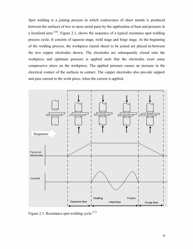
Spot welding is a joining process in which coalescence of sheet metals is produced

between the surfaces of two or more metal parts by the application of heat and pressure in

a localized area (16). Figure 2.1, shows the sequence of a typical resistance spot welding

process cycle. It consists of squeeze stage, weld stage and forge stage. At the beginning

of the welding process, the workpiece (metal sheet) to be joined are placed in-between

the two copper electrodes shown. The electrodes are subsequently closed onto the

workpiece and optimum pressure is applied such that the electrodes exert some

compressive stress on the workpiece. The applied pressure causes an increase in the

electrical contact of the surfaces in contact. The copper electrodes also provide support

and pass current to the work piece, when the current is applied.

Figur (17)e 2.1: Resistance spot welding cycle

Sequence

9

With electrical contact achieved by the effect of the electrode force, current is passed

through the sheet metals for a set time period. Heat is generated between the surfaces of

the sheet metals by the resistance offered to the flow of current. During this time a nugget

is formed in-between the plate samples (16) and grows further to become the spot weld as

heat generated by the resistance effect is sustained. After the weld is formed the applied

ressure is maintained to enhance solidification of the weld and to prevent expulsion. The

uring the welding process, once the specified cycle time which marks the process

ompletion is reached, the current supply is switched off and the weld (nugget) is allowed

solidify by slow cooling under pressure (16). The applied electrode force and the

surrounding solid metal help to contain the molten pool (16). The effect of the applied

der plastic deformation on the heated metal sealing creates a ring on

e surface of the metal. This effect can lead to corona (part with the ring impression)

xpulsion is accelerated when welding close to an edge due to bad fit or lack of

ode force (16). Expulsion can also occur at the

trode work interface if the generation of heat is too quick and excessive (16). This can

p

pressure is subsequently released and the electrodes are lifted away from the work piece (17). D

c

to

electrode pressure un

th

bonding (16). Expulsion occurs when this sealed ring ruptures suddenly during the welding

process such that some of the molten nugget metal is spewed out from between the sheets (16).

E

mechanical supports or low applied electr

elec

happen when scales which build up high resistance are present on the surfaces of the

sheets to be welded or when low resistivity metals are used (16).

The parameters which are considered in the spot welding process are electrode force,

diameter of the electrode contact surface, squeeze time, weld time, hold time and weld

current (18). These parameters will each be briefly discussed.

10

2.2.1 Electrode

The copper electrodes used during the resistance spot welding process plays a very

important role. The specific roles played by the electrode in the welding process are as

follows:

2.2.1.1 Electrode Force

2.2.1.2 Electrode Diameter

urface is used to determine the weld diameter. Weld

eter is a measure of weld quality. As the welding progresses the diameter of the

electrode will change eld diameter (nugget diameter) is

determ s that has been made with the electrode.

Generally the nugget diameter is slightly eter

A general recommendation (18) is that the weld should have a nugget diam

than 4

The electrode force is obtained by the compressive effect of the two electrodes applied to

the sheet metals thereby squeezing the metal sheets to be joined together (18). Adequate

electrode force is necessary to achieve good weld. The applied electrode force has some

inverse relationship with heat energy (18). Too low an applied force is inadequate for

achieving good weld quality. Excessively increasing the applied electrode force can lead

to expulsion (18). Optimum value of applied electrode force has to be determined for best

output.

Diameter of the electrode contact s

diam

due to effect of wear. W

ined based on the number of spot weld

less than the contact electrodes diam (18).

eter of greater

t t, (5 is recommended as appropriate), “t” being the thickness

sheet. However, the work done by Weber et al (19) gave further wear classes of electrodes

based on the num ith the electrode. Such that th

diameter should be based on wear state of the electrode. The wear classes, the num

corresponding spot welds and the nugget diameter that the weld should have as given by

of the steel

ber of weld spots made w e nugget

ber of

11

Weber s are pre nted in Table 2.1. Transitio state 1 p

Table 2.1 indicates the state of mild wear while transition state 2 is the state of rapid wear

f the welding electrode. In this research the electrode to be used is the one that has made

ore than 900 number of spot welds but less than 1700 (Wear class V1). So an achieved

meter

et al (19) finding se n resented in the

o

m

tdt 54 <≤ will be considered weld dia of satisfactory. Optimisation of the

sistance spot welding process however is to maximise the size of the weld diameter for re

a given set of input parameters.

Table 2.1: Definition of the wear classes (19)

Wear class Number of spot

welds

Quality Remark

V0 – non-wear state 9≤ 00 td 5≥ Spot weld is

“good”.

V1 – transition state 1 900 … 1700 tdt 54 <≤ Spot weld is

“satisfactory”.

V2 – transition state 2 1700 … 2000 tdt 43 <≤ Spot weld is

“adequate”.

V3 – worn state 2000≥ td 3< Spot weld is

“inadequate”.

2.2.1.3 Effect of Electrode Degradation

Many research and studies have been carried o t onu the degradation of electrodes during

sistance spot welding (20). Particularly because of the rapid wear of these electrodes re

with the increased usage of Zinc coated steels in manufacturing (20, 21). This has raised

production cost in the areas of frequent electrode change over time, cost of replacing

electrodes and high possibility for poor weld joint quality (21). Zinc coated steel protects

the steel sheet from corrosion (20).

12

Dupuy et al (20) reported a study on degradation of electrodes when spot welding zinc

findings of the study were that degradation of electrodes was

characterized by an enlargement of the electrode tip (20). This enlarged electrode tip

their respective studies mentioned that the actual cause

f electrode enlargement is still not very clear however, a number of phenomena are

given as the likely causes of the enlargement of the electrode tip. This ranges from

n of zinc into copper, possibility of pitting erosion, cracking of

lectrode tip, mushrooming and other reasons (20).

queeze time as shown in Figure 2.1, is the time at which the required level of the

rough the circuit (18). This is done to achieve good

lectrical contact between the electrodes and the work piece, and between the two

lates after

the squeeze time is completed as shown in Figure 2.1. Weld time is giving in weld cycles

with peaks and troughs such that one peak and a trough give a complete wave length. In a

coated steels. The main

causes current density passing through the electrode to drop and can get to a point where

the weld current is not sufficient to achieve a weld (20).

Dupuy et al (20) and De et al (21) in

o

possibility of diffusio

e

The importance of this electrode wear to this study is the fact that changes in the tip size

and topography of the electrode governs the nugget size and shape formation during the

welding process (20). Also, zinc coated metal sheet which is known to wear the copper

electrodes away so quickly are used for the experiment in this research. Electrode

condition is therefore an important quality consideration in the development of the

process model.

2.2.2 Squeeze time

S

pressure is set and no current flowing th

e

surfaces of the work piece (17, 18).

2.2.3 Weld time

Weld time is the duration in which the welding current is applied to the sheet p

13

50 Hz power system one cycle is given as 1/50 of a second (18). The welding time is

e in the welding process. Two half wave cycles gives

one cycle time , a number of halfwave cycle time are required to successively make a

rrent switched off,

d to the welded metal sheet for cooling. This period helps (18)

he weld current is made available in the welding circuit during spot welding by setting

window) for making the weld. Most spot welding

achine current tap switch are set so that between seventy and ninety percent current are

tilized (18). Determining actual current to use, is usually by trial and error, the guide is

heet metal, but has to be sufficiently high enough to achieve good weld (18) (should

curs between the metal sheets (18). This indicates that the correct

eld current has been exceeded. The lower boundary is the current that will be enough to

represented as half wave cycle tim(18)

spot weld. The total welding process time (program) to make a number of spot welds are

further divided into a number of small time steps (18). Typically the time steps are planned

(arranged) in such a way that they fall within the entire welding current window range

that will be used to spot weld a number of samples.

2.2.4 Forge time (cooling-time)

Hold time is the period from when the weld time is completed, the cu

and the electrodes still applie

the weld to chill as the nugget solidifies as shown in Figure 2.1. Optimum hold time is

necessary to prevent the electrode in contact with the hot spot weld heating up, or the

weld spot cooling too fast as it can alter the metallurgical property of the metal (18).

2.2.5 Weld current

T

the transformer tap switch to a level that allows a maximum amount of current to be

made available (18). The effective current used during the welding cycle is based on the

percentage of current set (current

m

u

that weld current should be kept as low as possible to reduce excessive heat input into the

s

achieve good weld diameter size as is practically possible).

When determining the current to be used, the current is gradually increased until weld

expulsion (splatter) oc

w

14

exceed the stick limit (18). Stick limit is the threshold weld diameter that is sufficient to

form a welded joint. This trial and error approach introduces much variability in the spot

weld quality and presents difficulty with reproducibility of the desired quality.

Having established the welding sequence in the resistance spot welding process, it is

important to investigate the previous techniques and methods that have been used for

modelling the process parameters.

2.3 Development of Resistance Spot Welding Process Control Models

This section presents the modelling and control approach used by previous researchers in

this area of study. Several techniques and procedures have been suggested for welding

process modelling, monitoring and control, involving routine or continuous monitoring of

the process variables.

Investigations on the development of real time control methodology by Tsai et al (22),

found that the initial approach to resistance spot welding modelling in the fifties was

ased on observing the electrodes movement during the welding process. Electrode

n

s

because the welding operation had to be interrupted to

ttach the thermocouples with an additional problem of spurious feedback signals and

b

displaceme ts were assumed to relate to the achieved weld size. Monitoring and control

equipment developed then was based on thermal expansion rate or maximum expansion

displacement (22). Other researchers continued to try improving on this model (22). This

lead to a number of monitoring and control equipment produced in this area but with little

or no success (22, 23, 24).

Progressing from the fifties to the sixties Tsai et al (22) reported J.A. Greenwood as having

developed a model that correlates the surface temperature of spot welds to maximum

temperature at the nugget centre during the welding process (22). In order to determine

temperature of the weld nugget using infrared emission from the metal surface,

thermocouples were mounted on either the workpiece or the electrodes (22). This approach

was reported as unsuccessful

a

15

erroneous temperature reading from the thermocouple due to variations in infrared

emissitivity (22).

Tsai et al (22) mentioned that to improve the monitoring and control process an automatic

trying to use the thermal expansion curve to adjust weld current, weld

e and electrode force, the electrode displacement in a number of cases were

ations (22).

g process and in service under

ading conditions. However, this optimisation procedure was limited and could not be

the earlier investigations temperature and pattern of formation of nuggets were calculated

load adjusting system was developed in the seventies by Johnson and Needham. This

system was based on the observation that by combining electrode force, weld current and

welding duration it will be possible to determine weld quality, provided a critical value of

applied electrode force was used. This system was able to restrict weld expansion during

welding (22). A linear relationship was said to exist between the subsized nugget and the

expulsion limit (22). Electrode force was at that stage presented as the most important

control parameter necessary to achieve good weld quality (22). The drawback as reported (22) was that while

tim

insensitive and sometimes had no response to the expansion signal in the initial expansion

rate based control system (22).

Further and more advanced techniques like ultrasonic signals and acoustic emission

techniques were employed to detect weld size (22). However, cost and complexity made

these systems unsuitable for use in most applic

Feng et al (3) gave a different perspective to the modelling and performance development

of the resistance spot welding process. He proposed an “integrated interdisciplinary

modelling approach to simulate the performance properties of resistance spot weld

joints”. The approach used basic physical phenomena such as the physics, mechanics and

metallurgy of the process, which occur during the weldin

lo

effectively applied to high-strength steels because weldment properties depend on

microstructure (3).

Further work in resistance spot welding process was in using numerical simulation

techniques to predict pattern and size of nugget during the welding cycle (23). In most of

16

without accounting for varying contact diameters at the electrode-workpiece surface and

the faying (surface of member that is in contact with another member to which it is

ined) surface between the sheet metals (23).

ontact diameter concept and observed interface

ontact resistance on the nugget formation process. The study applied varying contact

iameter model without incorporating contact resistance model and concluded that the

terface contact resistance can be ignored in normal resistance spot welding as it is not

po

g the nugget formation process .

as the recent work in 2002, by Matsuyama et al . In this new approach an algorithm

eters

wh

predict

measur

provide

jo

Matsuyama (23) reviewed the research work done in the mid eighties by Nishiguchi in

which the study produced a numerical simulation of nugget formation for estimating

contact diameters at the electrode-sheet interface. The review concluded that it was

possible to predict with some accuracy the nugget formation process without including

the electrical contact resistance at the faying surfaces (23).

In 2000, Matsuyama (24) developed a numerical simulation procedure to predict the

nugget formation process using varying c

c

d

in

very im rtant. The research work presented varying contact diameter alone as adequate

for estimatin (24)

An improvement to an earlier method that used a heat conduction differential equation(25)w

based on an integral form of an energy balance model for monitoring and control of the

resistance spot welding process was developed. The simulation was set to calculate the

average temperature of a weld during the welding cycle by using measured param

ich are welding voltage, welding current and total plate thickness. This was used to

both weld diameter and expulsion occurrence (25). Current and voltage

ements made across the electrodes were processed according to equation 2.1, to

dynamic resistance, given as (25):

IVR /= 2.1

here W R is the dynamic resistance (ohms), is voltage (Volts) and V I is current

(Ampere).

17

Only peak values of voltage and current were used in order to avoid the effect of

inductance (effect due to voltage drop in the circuit) on the value of these parameters (25).

Tsai et al (22) mentioned that the use of electrical parameters for monitoring and control of

the resistance spot welding process are considered the most successful of all in-process

quality control systems. However, there are a number of limitations (22), which are;

1. The method is mostly suitable for uncoated mild steels, compared to other metal

alloys and coated mild steels because of electrode wear during the welding

process, which makes reproducibility of same weld quality with the same machine

the

wear state of the electrodes to set boundary conditions.

d

oming weld quality prediction

uncertainty. Work by previous researchers in developing neural network application in

H wever, the extent has not been quantified in terms

f what quantity (value) of mechanical characteristics affects weld diameter (8). Tang et al

setting difficult (22). This can though be accounted for in a model, by using

2. The voltage clip position on the electrode to capture data during the welding

process gets on the way (22).

In these techniques, trial and error and experience still dominates its effective use (22)

particularly in the determination and setting of the welding machine for achieving desire

spot weld quality. Use of artificial intelligence applications like the artificial neural

networks are been used to model the resistance spot welding process (6). This application

technique is further explored in this research for overc

resistance spot welding are presented and extensively discussed in Chapter 3.

2.4 Effect of Machine Mechanical Characteristics on Weld Quality

Many researchers agree that welding machine mechanical characteristics does affect weld

quality with explanations on how. o

o(8) stated that the resistance spot welding machine is made up primarily of electrical and

mechanical subsystems which are believed to affect weld quality in some ways (8). Lipa (9)

mentioned that the resistance spot welding machine had always been viewed as a

18

transformer and its importance as far as influence on weld quality is concerned has been

the object of debates by many authors (9).

A recent work in 2003 by Tang et al (8) was carried out by experimental investigation on

welding machines using modified mechanical characteristics, which were welding force,

lectrode displacement, and other process characteristics, such as electrode alignment.

was made on the influence of the machine stiffness on the characteristics of

e welding force, electrode displacement, and electrode alignment. The work concluded

he study (8) also revealed that friction (condition of moving parts of the welding

h steel and aluminium welding. And in some

combinations of parameters because data ranges do overlap, the reduction in strength is

.

e

The identified characteristics were then linked to weld quality through process signature

analysis (8). Emphasis was placed on the signals during welding stage when electric weld

current is applied. Subsequently the hold stage was analyzed to see how it influenced the

solidification of the liquid nuggets (8).

From their study they found that machine stiffness (refers to the rigidity of the upper and

or lower arm of the welding machine part) slightly improves weld quality in terms of

weld strength and significantly raises welding expulsion limits (8). Further analysis as

reported (8)

th

based on the analysis carried out that “due to thermal expansion of the weldment, in a

stiff machine, the electrode force increases higher than its preset value to accommodate

the stiffness” (8). The increased electrode force imposes a forging force on the nugget,

which is beneficial for preventing welding expulsion (8).

T

machine) was unfavourable for bot

not statistically significant. The influence of friction was reported to vary with welding

conditions (8). The findings (8) were that the tensile-shear strength of welds and welding

expulsion limits, were not significantly influenced by machine moving mass (weight of

the cylinder head) for steel and aluminium welding alloys that were used for the

experiment. However machine stiffness and friction do affect welding processes and weld

quality (8)

19

Similar work was done by Satoh et al (26) and Dorn et al (27). These researchers have made

valuable contributions to the understanding of the effects of machine characteristics on

resistance welding. However, the results of these studies had been mainly descriptive (26).

The expressions of the influence are not explicit, but mostly comparative (26).

2.5 Concluding Remarks

ynamic resistance as presented by the recent work of Matsuyama (25) and others is

timately related to the progress of the welding operation. It is possible to obtain

formation regarding the nugget growth by monitoring the parameters that are related to

is variable. Dynamic resistance (varying contact diameter) therefore is a suitable and

ppropriate parameter that can be used for modelling and estimating the nugget formation

rocess.

The effect of mechanical characteri ality has been descriptive, not very

concrete and of some debate among researchers. Considering the unclear speculations

and debate around this issue, the possibility of using only

lectrical characteristics data to accurately predict weld diameter (weld quality).

meters data is thought to in some ways reflect the welding

state and mechanical characteristics of the welding machine.

D

in

in

th

a

p

stics on weld qu

this research will investigate

e

Electrical characteristic para

20

CHAPTER 3

NEURAL NETWORKS

3.1 Introduction

The chapter introduces the fundamentals of neural networks, neural network types,

learning rules, optimisation techniques and application in resistance spot welding process.

Neural networks controllers and the theoretical steps for the design of the process

ontroller are included in this chapter. Sensitivity analysis which is typically carried out

elson et al (30) gave the historical trend of neural networks development as having

c

in neural network modelling for determining the contributory effect of inputs to outputs

in a neural network model is discussed.

3.2 Background

Artificial Intelligence (AI) provides several techniques that are used in manufacturing

systems (28). In the 1980’s, knowledge based expert systems were the most popular

artificial intelligence techniques, they have however become less effective with the

continuously changing, complex and open environment of manufacturing systems (28).

Neural networks are identified as capable techniques that can be used in increasing

manufacturing system’s predictability because of its ability to learn, adapt and do parallel

distributed computation (28). Neural networks are robust systems (28). Smith (29) mentioned

that applying neural networks techniques in manufacturing systems creates potential to

increase product quality, improve system reliability and reduce the reaction time of a

manufacturing system.

N

started at conceptual level around 1890 with investigation and insights into brain activity.

The development progressed to 1936 with the successful explanation of the brain as a

computing paradigm by Alan Turing (30). This explanation gave a deeper insight into

21

neural network concept. In 1943 Warren McCulloch and Walter Pitts presented a work (30) explaining how neurons might work by modeling a simple neural network using

electrical circuits. This discovery by Warren McCulloch and Walter Pitts was used by

John von Neumann for teaching theory of computing machines (30). In 1949, Donald

Hebb presented the connection between psychology and physiology and explained how

neural pathway is reinforced each time it is used (30). Following the improvement on

hardware and software capability in the 1950s, research in this area progressed further.

he period 1969 to 1981 recorded stunted growth because of reduced funding and

diverted attention to artificial intelligence that looked more promising at that time (30).

iteratur (28, 31) described the basic components of a neural network as nodes (or

h the n

eural networks as having the capability to solve problems without a detailed, explicit

Hassoun

as pattern rec tion, through a learning process. The research

further des b

from complica t patterns and detect trends which are too

com humans or other computer techniques (31).

T

However from 1982 to date there was a marked turn around and renewed interest in

research in the field of neural network and a period of unfolding application possibilities

mostly due to the availability of capable computer hardware and better understanding of

neural network capability (30).

L e

neurons, adapted from a biological neuron) and adaptable weights (31). These neurons are

also referred to as processing elements (28, 31). Weight in neural network refers to the

adjustable parameter on each connection that scales the data passing through it (31). The

weights were presented by Hassoun (31) as corresponding to biological synapses.

Identified inputs referred to as signals are accumulated and put throug etworks,

adapted by the weights, and the sum passed to an activation function that determines the

neurons response (31). Neural networks learn by example (31). Hung et al (28) presented

n

algorithm available for the solution procedure.

(31) mentioned that a neural network is configured for a specific application, such

ognition or data classifica

cri ed the neural network as having a remarkable ability to derive meaning

ted data and is able to extrac

plex to be noticed by either

22

Martin (32) 80's that have

made grow o first was reduction

in t n umber of inputs. This was achieved by the basic change

in the learn

on the devel t of “inverted” or “reversed” neural networks (32). These two

entioned breakthroughs have helped with solutions for large scale problems involving

me series models and nonlinear multiple-input-multiple-output (MIMO) models (32, 33).

rincipe et al and other authors (34, 35) listed what makes a neural network unique as

pt to changing conditions online

• Universal approximators

– They can learn any model given enough data and processing elements and

time

.2.1 How Artificial Neural Networks (ANN) Work

eondes (35) reported the work carried out on universal approximation theorem in 1984 by

e research group in San Diego which described neural networks as a heuristic technique

unsupervised learning paradigm.

ation

reported two breakthroughs in neural networks use in the late

th f the application possible in the process industries. The

rai ing time even with large n

ing algorithm. The second was a deeper insight by the work of Caudill et al (33)

opmen

m

ti

P

follows:

• Nonlinear models

– Many nonlinear models exist, but the mathematics required is usually

involved or nonexistent.

– Neural networks are a simplified nonlinear system (combinations of

simple nonlinear functions).

• Trained from the data

– No expert knowledge is required a priori

– Each task does not need to be completely specified in code

– They can learn and ada

3

L

th

used to perform various task within the supervised or

This consists of optimized training, selection of appropriate size of a network and

prediction of how much data that are required to achieve particular generaliz

23

performance. The sequence in using artificial neural networks consists of determining the

input and output signals (34, 35). This is followed by using generated data set to train and

validate the network. A neural network architecture made up of inputs, network layers

with hidden layers and output is shown in Figure 3.1. Hidden layers are the layers in-

between the input and output layers.

igure 3.2: Neural Network Adaptive process (34)

Hidden layers

Input

Input Output

Input

Figure 3.1: A neural network architecture [adapted (34)]

At the training stage, the data is presented to the network (34). Figure 3.2 shows the

adaptive process which takes place during the training stage of the neural network.

F

24

The network computes an output which is compared to the desired output. Based on the

ssing the epoch through an

iteration process. An epoch is a complete set of input/output data made up of elementary

and e mentary is

a comp

showin

(34)]

To use the network a new set of data different from a test set are used to validate the

network. The network then computes the output based on its training (34). The various

aspects of the Neural Network models are as follows (35, 36):

• Neurons

• A state of activation for every unit, equivalent to the output of the unit.

• Connection between the units: each connection is defined by a weight which

determines the signal of the unit.

• A propagation rule: determines the effective input of a unit from its external

inputs.

• An external input or bias (threshold) for each unit.

• A learning rule and an environment within which the system should operate.

level of error (difference between computed output and desired output) referred to as cost

in neural network terms, the network weights are modified (adapted) to reduce the error (34) see Figure 3.2. The weight modification is done by pa

ex mplar. An exemplar is one individual set of input/output data while ele

lete set of input row. Presented in Figure 3.3 is a single neural network structure

g these terms.

Inputs Weights

Ele n

Figure 3.3: Single Layer Neural Network Structure [adapted

5, 3, 2, 5, 3

1, 0, 0, 1, 0

5, 3, 2, 2, 1

Outputs

5, 3, 2, 5, 3 me tary

Exemplar

25

In a neural network structure as is shown in Figure 3.4, the processing element (neuron)

has one scalar input (p) transmitted through a connection th

26

at multiplies its strength by

e scalar weight (w), to form the product (wp), again a scalar (36).

Figure 3.4: The Sim (36)

Here the weighted input ly argument 36) of the transfer

function (f), which produces the scalar output ( ) such that:

(3.1)

put and thus more than one

weight such that the parameters can be adjusted for the network to exhibit some desired

ehaviour (36). This creates the possibility for a network to be trained to do a particular job

th

ple Neuron Model

(plus the scalar bias (b) are the on

a

)( bwpfa +=

This sum is the argument of the transfer function f . The parameters w and b are

adjustable scalar parameters of the neuron (36).

It is possible for a single neuron to have more than one in

b

by adjusting the weight or bias parameters (36).

Many artificial neural networks (ANN) can be considered function approximator (34, 35).

Function approximation approximates the function f when y = f(x), given y and x (input

& o

binary (on or off)

Art i

learning machines

Artifici nctions to approximate complex

fun (34) ceptron (MLP) and radial basis function

BF) which will be discussed in later section, the MLPs approximates input-output

Huang entioned that neural networks are being applied in many fields. Some of

the ben t

•

• rning and adapting ability.

• is robust, accurate and can operate in real time.

• ors for space-constrained and power-constrained applications.

• t antly reduced.

• quickly and accurately solve difficult process problems that cannot be

• t such that small changes in an input

• training data set.

utput respectively) (34). Examples are:

– Linear regression

– Classification, where the output function is

ific al neural networks are good for function approximation because

– they are universal approximators

– they are efficient approximators

– they can be implemented as

al neural networks use ensembles of simple fu

ctions . For example in multilayer per

(R

function using a combination of functions like logistic or tanh while RBFs approximates

input-output function using a combination of Gaussians (34).

3.2.2 Benefits and Applications of Neural Networks

et al (28) m

efi s as given by Huang et al (28) are as follows:

High processing achieved through massive parallelism.

Efficient knowledge acquisition through lea

It

Compact process

Da a analysis tasks time is signific

It is able to

solved with conventional methods.

In the presence of noise the nets are robus

signal will not drastically affect a node's output.

Can generalise from

27

Smith

manufactu process planning, scheduling, process

monito g

Artifici n n applied in the following areas (37, 38):

usiness

to evaluate the probability of oil geological formations

forecasting

• For assessment of credit risk

•

• Analysing portfolios and rating investments

a

Automating robots and control systems (with machine vision and sensors for

a)

• Controlling production line processes

anding cause of epileptic seizures

(29) reported that neural networks have been implemented in broad areas in

ring, including the design phase,

rin and quality assurance.

al eural networks have specifically bee

B

• Used

• For Identifying corporate candidates for specific positions

• Recognition of hand written signatures

Environmental

• Used for weather

Financial

Identifying forgeries

M nufacturing

•

pressure, temperature, gas, etceter

• Inspecting for quality

• Selecting parts on an assembly line

Medical

• Analysing speech in hearing aids for the profoundly deaf

• Diagnosing/prescribing treatments from symptoms

• Monitoring surgery

• Predicting adverse drug reactions

• Reading X-rays

• Underst

28

Military

mentioned that it is only recently, that neural network techniques are

finding its way into the industries (39) (39)

problem

unstable when applied to large scale problems . This as explained by Yalcinoz was

due to th

conditions and inefficient m ine weights in the energy

function”. Yalcinoz

improve odifying the algorithm, such that

Presently, a lim

boxes whose rules are unknown. Results are

explainable m (41)

means is that while it presents an accurate representation is

unclear and is not yet well understood

Some other disadvantages of neural networks , which hinder the optimal application

of neural networks in certain areas, are:

Use of trial and error methods to find the proper neural network architecture for a

given problem. This makes it usually time-consuming; this is though improved

• Classifying radar signals

• Creating smart weapons

• Optimising the use of scarce resources

• Recording and tracking targets

3.2.3 Neural Networks Limitations

(39) Stergiou et al

. According to Stergiou et al , one of the major

s with neural networks in the early times was that neural network programs were (40) (40)

e “network solution having a local minimum which depends on the initial

apping method used to determ(40) explained that the limitation was however overcome by an

ment in the energy function. This was done by m

reliable feasible solutions were produced and various methods developed to escape from

the local minima.

itation that is yet to be overcome is that neural networks function as black

presented as output without giving

athematical function that was used to arrive at the answer . What this

output result, the knowledge(41).

(29, 37)

1.

with the use of genetic algorithm.

29

2. Sometimes a particular neural network learning algorithms for a given problem

may not be efficient enough for network convergence.

3. Acquisition of an optimal training set for a specific neural network application

continues to be a challenge.

For neural networks to be used more effectively, there should be improvements in the

following areas (37):

1. In knowledge representation, non-numerical operations, and symbolic reasoning

Specifically compared to the neural

techniques in solving the complex non linear resistance spot welding process modelling

ar and

ynamic process like the resistance spot welding process is the ability to learn and track

which are areas that basic neural networks cannot deal with.

2. The determination of number of nodes, number of layers, connections, and initial

weights of a neural network should be easier.

3. Possibility for determining the optimal network architecture while training by

controlling the minimal number of nodes, weights, and layers during training.

While these limitations do not pose an immediate problem, overcoming them will

make the technique more usable (37).

3.3 Neural Networks versus Other Methods

In this section neural network technique is compared with other methods used for the

analysis and design of models and control systems.

network techniques are the traditional linear statistics method that has been in use for

long and the more recent techniques like fuzzy set theory and program algorithm. The

reason for comparing, is to justify the appropriateness of the use of neural network

and control problem.

A very useful capability of a predictive modelling tool in a chaotic, non line

d

changes (41). Linear statistics are able to model nonlinear variables but do not have

learning capability to track dynamic systems, compared to neural networks that are able

30

to learn and recognise patterns in complex, dynamic and chaotic events (41). Neural

networks can create their own organization or representations of the information received

during learning, with additional ability to represent any function and learn from

representative examples (41). This capability has made neural network useful and superior

to linear statistics and many other non-statistical techniques (41). In addition to this

capability, neural networks because of its robustness can tolerate partial destruction of its

network, though this could lead to a corresponding degradation of performance, some

network capabilities can however, still be retained even with major network damage (42).

This robustness is absent in linear statistics method.

al networks techniques (41, 42). Neural network systems are stable.

eriority of neural networks to other

ethods is the fact that it is extremely sensitive to noise or unreliable data. There is no

tion on the output type (41). Neural networks can output results of complex

e (43). Neural networks

that it has not seen before, it generates a reasonable response. Most

to accurately generate a reasonable response in most non linear, c

relationships (41, 43).

Fuzzy set theory is a technique that can be used like the neural network. Fuzzy set theory

was developed with the capacity to deal with problems which were not solvable with

traditional statistical methods (42). However, the use of fuzzy set theory requires a good

knowledge of rules for modelling a process, and sometimes closed-loop systems

developed using fuzzy logic are unstable (42). This burden of the knowledge of rules is

absent with neur

Neural networks models are predictive (models are accurate with reality) even though

they are not descriptive (41). It is possible with neural networks to go straight from data to

the model without the need for extra tools like recoding or simplification. This is not

possible with other methods (41). Additional sup

m

restric

processes in a short computational time and can be done in real tim

are able to generalise (41). That is when a trained neural network is presented with data

methods are not able

omplex and chaotic

31

Other methods on handling data have many drawbacks which neural networks do not

possess (43). For instance statistical techniques imposes restrictions on the number of input

data compared to neural network that can accept as much inputs and outputs as possible

in a single netw

32

ork architecture. The regressions performed with statistical methods

mostly uses simple dependency functions (linear and logarithmic), which are quite

unrealistic (43).

Statistical techniques require intensive mathematical methods to transform data; this is

not needed in the use of neural network techniques. Neural networks are non-linear hence

are better able to account for complexity of human behaviour and real life situations (43).

nd they can give tolerance to missing values (41).

Figure 3.5: A Simple Feedforward Neural Network Diagram (39).

A

3.4 Classification of Neural Networks

The two major kinds of network structures for the neurons making up the neural networks

are feedforward and feedback network structures (43). Feedforward neural networks are

biologically inspired classification algorithm made up of a number of simple neurons

organised in layers (44). The signals can only travel in one direction from input to output.

There is no feedback (39). Presented in Figure 3.5 is an example of a simple feedforward

neural network.

The layers arrangements are such that every unit layer is connected to all the units in the

previous layer and each connection has a different strength or weight (44). The weights on

these connections encode the knowledge of a network (44). There is no feedback between

layers when it acts as a classifier (44). This is because data enters at the inputs and passes

through the network, layer by layer, until it arrives at the output (s). Feedforward neural

networks usually produce a response to an input quickly (43). Most feedforward neural

networks can be trained using a wide variety of efficient conventional numerical methods

in addition to algorithms invented by neural network researchers (43).

Feedback neural networks are network structures where every neuron is potentially joined

to every other neuron (46), such that the output of one layer routes back to a previous layer (45) forming cycles among the neurons in the network connections (43) as is shown in

Figure 3.6. They have signals travelling in both directions (43).

Figure 3.6: Simple Feedback Network Diagram [Adapted (45)]

Feedback

Hidden layer

Inputs Outputs

Feedback

33

Another unique behaviour of feedback neural network is its ability to update the

activation of all neurons in parallel (46). In some feedback neural networks, each time an

put is presented, the neural network must iterate for a potentially long time before it

eural networks are also classified as supervised or unsupervised based on the training

rning the inputs and outputs are provided,

nd an input – output relationship is established. What this means is that the network

what

ill use to group the input data (42, 48).

an al distinct neural network models

their internal architecture and from the learning

ral Network Architectures

ultilayer perceptron (MLP) architecture is a supervised neural network type with

edforward network structure where each unit receives inputs only from a lower layer

in

produces a response (43, 47). Feedback neural networks are usually more difficult to train

than feedforward neural networks (43). It is possible to control the connections between

the neurons (45). Also, by changing the parameters that controls the connections (45) the

neuron in the network can be excited or inhibited.

N

(teaching) method used (42). In supervised lea

a

processes the inputs and compares the resulting outputs against the desired output. While

for unsupervised learning, only inputs are provided with no desired output. The neural

network then decides for itself through a process of adaption or self organization

features it w

There are m y classes of neural networks (42). Sever

can be distinguished both from

algorithms that they use (48). Neural network architectures, learning algorithms, training

and neural network controller model are further discussed.

3.4.1 Neu

Different kinds of neural network architectures exists (48). The most commonly used ones

are Multilayer Perceptron (MLP), Radial Basis Function (RBF), Self Organising Map

(SOM) and Recurrent Neural Network (RNN). These are discussed in this section.

3.4.1.1 Multi-layer Perceptron (MLP)

M

fe

34

unit (34, 49). The network is termed supervised because desire targets are presented to the

network during training. MLP are powerful models for solving nonlinear mapping

problems.

The simplest network architecture consists of a single layer with directed inputs and

weighted connections to the output unit (49). The network is trained with standard

backpropagation (simple learning algorithms which finds the weights for linear and

binary activation functions) algorithm (34). However, these algorithms can only work for a

limited number of functions. The limitations are overcome by adding one or more layers,

known as hidden layers which are nonlinear units between the input and the output (44, 49).

Presented in Figure 3.7 is a typical architecture of a multilayer perceptron network.

Input Layer

Hidden Layer

Output Layer

Figure 3.7: Architecture of a multi-layer perceptron network (50)

As shown in Figure 3.7, in the hidden layer is a nonlinear node with an elementwise

nonlinearity function and the output layer with linear node. The computations performed

35

by the network with a single hidden layer with nonlinear activation functions and a linear

output layer can be written mathematically as (50):

Bsfx == )( baAs ++ )( (3.2)

where s is a vector of inputs and x a vector of outputs. A is the matrix of weights of the

first layer, a is the bias vector of the first layer. B and b are the weight matrix and the

bias vector of the second layer respectively, is the weight parameter.

Hagan et a (36)l xplained that the principle of the network operation is that the network

odes perform calculations in successive layers until an output value is computed at each

value represented with ones on the

orrect class node and a low output value on all the rest represented with zeros (36).

ne ork computation is the squared

ifference between the actual and desired outputs. The activities for each unit are

comp forward ation thr network, arious training cases.

Starting with the output units, backward propagation (chain rule) through the network is

used to compute the derivatives of the error function with respect to the input received by

each unit (36, 49).

e

n

of the output nodes. This happens when data from an input pattern is presented at the

input layer. Each layer of neurons may have a different number of neurons and a different

transfer function (36). The output of the MLP is expected to indicate the appropriate class

of the input data. That is there should be a high output

c

The error function generally used in the neural tw

d

uted by propag ough the for v

The learning algorithm and number of iterations determines how good the error on the

training set is minimized while the number of learning samples determines how good the

training samples represent the actual function (36). The different kinds of activation

functions with their equations are shown in Table 3.1.

36

Table 3.1: Different Types of Activation Functions (36).

Name Linear Sigmoid Tanh Softmax

Function

A

( )ae−+11

( )( )aa

aa

eeee−

−

+−

∑j

aj

a

ee

Perceptron learning rule is used in MLP. This learning rule is a method used for finding

the weights in the network (49). The perceptron has the property of searching for the

existence of a set of weights which it uses to solve a problem (49). This rule follows a

linear regression approach, that is, given a set of inputs and output values, the network

finds the best linear mapping from inputs (49)

(

to outputs . Based on training, the network

an predict the most likely output value 49). This ability to determine the output for an (36, 49)

provided a sufficient number of hidden units are (36)

ximation with BiasAxon or LinearAxon

the transfer function. Each processing element in the Multilayer Perceptron

ward pass . In the forward pass

, given inputs are used to predict output. In the backward pass, it is explained (50) “that

e partial derivatives of the cost function with respect to the different parameters are

c

input the network was not trained with is known as generalization .

Multilayer perceptron networks are known as approximators (two-layer networks with a

sigmoid transfer function in the hidden layer and linear transfer functions in the output

layer) and can approximate any function (36)available . These hidden units make use of non-linear activation functions . The

performance of MLP function approximation does not degrade with increased input

dimensionality unlike polynomial based function approximators (34). Linear output is used

for the multilayer perceptrons for function appro

as

architecture contributes to the global function of the network. A change in one weight

may greatly affect the global function (34).

The back-propagation algorithm used for solving learning problem of the MLP can take

two forms; the forms are either forward pass or back (36, 49)

(50)

th

propagated back through the network”.

37

The same chain rule of differentiation which gives similar computational rules for the

o-associative structure, a process of

etting the same values for both the inputs and the outputs of the network (50), such that

ator for

(51). The

and chaotic time series prediction (52).

The RBF architecture consists of two-layer fully connected network, with an input layer

Figure 3.8: Radial basis function (RBF) network (52)

forward pass is same one for backward pass (50). The network adapts weights by using

any gradient-based optimisation algorithm (50) and the iteration of the whole process is

continued until the weights have converged (50).

Though the MLP is a supervised neural network type, it can also be used for

unsupervised learning. This is done by using aut

s

the extracted sources can emerge from the values of the hidden neurons. This process

approach is however computationally intensive (50).

3.4.1.2 Radial Basis Function Networks

The radial basis function (RBF) neural network is a universal approxim

continuous functions given a sufficient number of hidden units. RBF have proven to be

valuable alternative to multilayer perceptrons (MLPs) in many real world tasks

tasks include speech recognition, data classification

performing no computations (51, 52). See Figure 3.8.

wKwbw1

f(ξ)

s1(ξ) sb(ξ) sK(ξ)• • • • • •

ξ1 ξi ξN• • • • • •Input layer

Hidden layer

Output layer

38

RBF is a commonly used neural network type (52). The computation nodes of the hidden

layers of radial base function network are different and serve a different purpose from the

utput layer of the network as opposed to the MLP where the hidden and output layers

share a common neuron model (52).

while the output layer is linear. This makes the network unable to approximate non-linear

nctions compared to MLP in which both hidden and output layers are non-linear (51, 52).

The outputs are linearly combined with weights, w1, w2,

wb,…wK, in the output layer of the network, f(ξ) (52). The general output of a RBF

etwork is thus (52):

(3.3)

utput tails off as the input value moves away from this point (51). The most commonly

applied transfer function of an RBF network is the Gaussian and the output of the

o

The hidden layer of the RBF network is non-linear

fu

Radial basis function networks are feedforward neural networks. The distinguishing

feature of an RBF network from other networks is that RBF network uses radial functions

(i.e. the transfer functions of the hidden units) while other neural network types does not (52). In the RBF structure each of the components of the input vector (ξ) feeds forward to

the basis function (K).

…

n

∑=

=K

bbb swwf

1

)(),( ξξ

where ξ is the vector applied to the input neurons and sb represents the transfer function

(basis function) b. RBF hidden layer neurons have a receptive field which has a centre:

that is, a particular input value at which the neurons have a maximum output (52). Their

o

network is given by (52):

∑ ⎟⎟

⎠

⎞

⎜⎜

⎝

⎛ −−=

=

K

b b

bb

mwwf

12

2

2),(

σξ

ξ (3.4)

39

where each hidden node is parameterized by two quantities: a centre m in input space and

re neurons than most other neural

akes it very unique (53).

(54). The SOM

(also known as the Kohonen feature map) algorithm is one of the best known artificial

o using

upervised learning, the SOM is based on unsupervised learning (54). In this unsupervised

he SOM can thus serve as a clustering tool of high-dimensional data. And can construct

topology preserving mapping from the high-dimensional space onto map units in such a

ay that relative distances between data points are preserved (56). The map units, or

eurons, usually form a two-dimensional regular lattice where the location of a map unit

ies semantic information (55, 56), See Figure 3.9. It is made of a number of neurons

width σb (52). Generally radial basis network requires mo

network types (36). Its simple structure and fast learning ability m

3.4.1.3 Self-Organizing Maps (SOM)

Self-Organizing Map (SOM) was introduced by Teuvo Kohonen in 1982

neural network algorithms (54). In contrast to many other neural netw rks

s

learning the network performs some kind of data compression, such as dimensional

reduction or clustering (48) by visualising high-dimensional data and converting it into

simple low – dimensional display as is shown in Figure 3.9.

Figure 3.9: Dimensional Reduction of Data by Self-organising map [adapted (31)]

T

a

w

n

carr

40

that are arranged in a predefined structure (56). In most cases this structure is a regular

rid of neurons of 1-, 2- or 3-dimensions (56).

SOM neural network type is relatively easy to implement and evaluate, and is

omputationally not expensive (54). However, it has the problem of overcrowding and

e to the size and shape of the network

at are fixed before the training phase begins (51, 55). Presented in Figure 3.10 is a Self-

igure 3.10: Self-organising map architecture (31)

he weight of each processing element (PE) represents the center of its cluster as is

sion of the input vectors 4). In essence the reference vector consists of the weights of the neurons. The reference

vectors together form a codebook. The neurons of the map are connected to adjacent

g

c

underutilization of the neurons in the network du

th

Organising Map architecture.

PEs

Neighbors

weights

inputs

F

T

shown in the Figure 3.10. Neighboring PEs has similar weights.

The SOM identifies a mapping from high dimensional input data space onto a regular

array of neurons (54). Every neuron i of the map is associated with an n-dimensional

reference vector [ ]Tll mmm ln1 ,,K= , where m denotes the dimen(5

41

neurons by a neighbourhood relationship, which dictates the topology, or the structure of

the map (57). The most common topologies in use are rectangular and hexagonal topology (57). SOM is most suitable for classification problems as such will not be used for the

application problem being investigated in this research.

3.4.1.4 Recurrent Neural Networks

Recurrent networks can have an infinite memory depth and thus find relationships (34)

ation, and temporal pattern classification

. The human brain is a form of recurrent neural network (58).

Recurrent neural networks are a kind of network with feedback connections (58). They are

computationally powerful and because of their ability to implement almost arbitrary

behaviour they have found good use in adaptive robotics, music composition, speech

recognition and other applications (58). Backpropagation algorithm which is one of the

best learning algorithms can not be easily used in the recurrent neural network

architectures. This is because to use backpropagation algorithms in a network, the

architecture has to be of feed-forward form (34, 51). This adds some comput tional

expense.

re lengthy sequence of vectors making

andling of the input and outputs sometimes difficult to follow through (51). Presented in

through time as well as through the instantaneous input space . Most real-world data

contains information in its time structure. Recurrent networks are the state of the art in

nonlinear time series prediction, system identific(34)

a

The inputs and outputs of this architecture a

h

Figure 3.11 is a fully recurrent neural network.

42

ork entails finding the network parameters (weights and biases)

ate a given function (48). Neural networks have the ability to

When training the neural network, care is taken to ensure that they do not overfit the

training data as this can prevent the network from generalizing (48). The process is as

Figure 3.11: Fully recurrent neural networks (59)

Fully recurrent networks provide two-way connections between all processors in the

neural network (59). They are typically complex, dynamical systems, and exhibit

instability (59). Having, discussed the classification and architecture of neural networks.

The next section is about how neural networks are trained.

3.4.2 Neural Network Training Methods

Training the neural netw

which would best approxim

learn from examples by adapting the weights on its connections in order to achieve a

desired specification using specific learning rules (48). During the learning process, the

network embodies the complex relationships between the network inputs/explicative data

and the network outputs/explained data (48). This learning process produces a statistical

model which can determine an estimation of the likely outcome when fed with an input

variable (48).

43

follows: E

propagated tow

are either the . The prediction obtained at the network’s

output is c d

the difference

the network gives) are computed. This error value is then backpropagated by going

upwards in e

contribution of

the learning se

are

known (48) ghts and corrects mistakes by modifying

the weight twork

form, wher y

nodes as anoth

rules are as fol

- Biologically based rule such as Hebb’s rule – one of the learning rules in

ion (input) (60).

tion which allows networks to adapt to changes in input data over

g Law – an unsupervised learning rule, used when

tem, via the Kohonen clustering algorithm, which

The practical

criteria during pping criteria include (34):

Using fixed number of epochs.

ach example (data) is entered as input in the neural network. The values are

ards the output through a function. These are activation functions which

linear, logistic and softmax (48)

alle an error or cost function (48). As explained earlier, the error value which is

between the expected value (real output) and the actual output value (what

th network and modifying the weights of each hidden unit based on the error

each to the total error value. This mechanism is repeated for each value in

t (48).

Neural network uses trial and error method of learning and finds the patterns associating

inputs and outputs using a large set of training data where both inputs and outputs

. It initially begins with random wei

that it has given each input item (48). The network works in feedback ne

eb a given node output can be transmitted back to itself or to other previous

er input (48). The learning process is done using models and rules (48). These

lows:

which changes in synaptic strengths (weights) are proportional to the

neuron activat

- Grossberg Learning – a learning rule based on self-training and self-

organisa

time (61).

- Kohonen’s Learnin

breaking down a sys

takes a high-dimensional input and clusters (55).

approach to training a neural network is to know how to set stopping

the training of the network (34). Common sto

–

– Stop when the mean square error (MSE) gets below a certain point.

44

– Use of cross validation criteria to monitor performance. Cross validation

rmance and not necessarily

• Trying many possible networks and using the smallest network that meets the

• Use at forces weights (discriminant functions) that

• validation by :

– setting aside a subset of data to test the network

• If too slow, network will not be able to make accurate predictions.

method).

In decision based neural networks, the target determines the correctness of the

clas i g pattern (41). The objective of the learning process is to find

helps to store best weights that gives best perfo

for stopping the network.

The aim during the training process is to maximize generalization (34). The following can

be done to achieve this (34):

design criteria.

of weight decay – a method th

are not necessary to zero.

Use of cross

– Monitoring the network to avoid memorizing. Memorizing occurs when

the training set mean square error (MSE) continue to fall while the cross

validation mean square error starts to rise.

The learning process is a trade-off made between the training speed and the weight

quality (degree of error or convergence) (48).

• If too fast, weights may not be effective for new data.

There are two approaches to learning in supervised training (48). The approaches depend

on the nature of the target values which are (42, 43):

1). Based on the correctness of the decision (how accurate the results are

compared to the target values).

2). Based on the optimization of a training cost function. (The least square error

sif cation for each trainin

45

a s o at gives an accurate classification (42). In the first phase (retrieving

phase) the objective is to determine which class the pattern belongs to based on the output

values. The output values are function of the input values and network weights (41, 42). The

learning process sequence consists of the input data propagated through the network to

ard through the

etwork. Depending on the level of error the weights are modified accordingly (42).

rks, the correctness of the training pattern is

etermined when the error or cost function has been minimised. This function is

er, the function to be minimised

ight be subjected to constraints in the form of equality constraints or bounds (47, 62).

• Descent Optimization

Inverse Neural Network

that can learn the inverse of

et f weights th

compute the system output. Error is computed and propagated backw

n

In optimisation based neural netwo

d

minimised by using the least square error method of optimisation (41, 42). The optimisation

technique is used to find a set of design parameters (44, 49), that can be defined as optimal (44). This could be in order to minimise or maximise a particular function such as an error

function which is dependent on another variable. Howev

m

The optimization techniques used include the following (44, 49):

• Inverse Neural Network

• Brute-Force Method

• Fminbnd

• Quasi-Newton Methods

A discussion of each of these optimisation techniques are given below.

3.4.2.1

The role of an inverse neural network is to predict the unknown inputs to a system such

that it can produce a desired output. Psaltis et al (63) proposed mathematical algorithms

target system mappings for the purpose of predicting

unknown system inputs to produce the desired outputs.

46

Psaltis et al (63) explained that in many real cases, learning the inverse of the system by

mathematical algorithms was very difficult and time consuming. This complexity of

mod i the derivation of inverse nonlinear mapping

from on (MLP) or radial basis function (RBF)

whi i system (64, 65)

Williams and Linden et al developed the first methods of inverting feed forward

neural n

based o h method (similar to back-propagation) in

whi a utput

and

The use

neural

process uct quality control problems as well as simple predictions

. To use inverse neural networks the target values take the role of the input while the

ell ng direct inverse systems has led to

a simple neural network multilayer perceptr

ch s trained as a simulator of a given .

(66) (67)

etworks. It was an inversion algorithm of feedforward neural networks which is

n numerical gradient descent searc

ch candidate inverse is iteratively refined to decrease the error between its o

the target (66, 67).

of inverse neural networks has over the years emerged as a useful technique in

network application (34). Inverse neural network models are used for solving

optimization and prod(34)

input takes the role of the target values. Upon training the network a relationship of the

output-to-input is obtained rather than input-to-output. This can then be used to adapt the

network to correct the output to the required output. The algorithm is as shown below (34):

• Desired output value, yd is entered

• The current position, yact is also entered

• The difference between the two, actd yyy −=1 is obtained

• The absolute of this difference is )( 12 yabsy = required to update the position.

This absolute is passed through the inverse neural network to get the required

input, x which gives this position. 1

• This input is then passed through the neural network to get the position, y3.

• y3 is compared with y2 while updating the input value, until the point where the

two are equal or less than an error value. This input is then returned as the

required input value which would set the actual output value to the required

output hence minimizing the difference between the two, which is the

optimization process.

47

An obvious problem associated with network inversion arises when a many-to-one

ulation requires a large computational cost to find an exact inverse of the target

ven on neural networks of moderate size (31, 69). Inversion therefore, only yields estimate

verses which approximate the inverse of the target to a certain degree (69).

Additionally, the use of inverse neural network optimisation technique takes a long time (69)

ques or algorithms that have been developed for (28)

.

.4.2.2 Brute Force Method

the end of the data range set . Different values of the input are then tested until at the

than the in e err alue . One major drawback of this technique is that in

m f ut values are created with incremental steps chosen as a

function must invert from one to many targets (31, 68, 69). What this means is that in a

typical neural network structure a number of input variables are used to generate one

output (31), whereas in Inverse neural networks model it is required that the output be used

to determine the inputs. While this is possible it could be very difficult (68). The

manip

e

in

to find the optimal position, hence would not be practical for a large data training set .

The reason it takes a lot of time could be attributed to the fact that if the signal is a

random signal or a non-linear relationship the value could lie within a small range such

that the method keeps fluctuating around this point (due to the gradient of search) (31, 69).

This disadvantage makes this technique inappropriate in the resistance spot welding

process modelling problem.

There are though several techni

improving inverse neural network accuracy . These algorithms are based on fields

such as numerical optimization methods (e.g. gradient descent search method and

nonlinear programming) and other methods such as fuzzy logic and evolutionary methods (28)

3

In this method input arrays and values are defined from the start of the data range set to (44)

point where a particular input value gives the required output or an output less or greater

put by th or v (44, 47)

the algorith an array o inp

48

result if the i it is too small ncrements are too large the solution would be skipped and if

e method would converge too slowly (47).

Sim he array, it would take a lot of time before

find g the array is too small the solution would

not s reason that this method is discouraged.

3.4 3 imisation Technique (Fminbnd)

This m box (47). The optimisation technique is a mean

quare error minimisation function (47). The function is minimised by finding the

th

ilarly, if there are too many inputs in t

in the possible solution and if the input in(47) be found for small accuracies . It is for thi

.2. Bounded Min

ethod is from the MATLAB 6.2 tool

s

optimum parameter that gives the minimum turning point(s) of the function to be

minimised or the minimum point of the function within bounds specified for the

parameter (47). Such that (47):

[ ] ),,,(@fminbnd,,, OptionsxxFunOptionsExitflagFvalX UL= (3.5)

where:

• Fun is the function to be minimized

•

• eter

• acy and displays what the function should

do.

xL is the lower bound for the parameter

xU is the upper bound for the param

Options can be used to specify the accur

• X is the optimum value

• Fval is value of the function

• Exitflag is a convergence criterion.

This optimisation technique returns the optimum value onto X, the value of the function

at this optimum value is also returned to fval. It is reported (47) that the Exitflag takes on a

49

value of 1 if the method converges, 0 if it does not converge and -1 if the number of

iterations is exceeded.

This method however has the following limitations (70):

• The function to be minimized must be continuous.

ns.

Fminbnd only handles real variables.

ses either the Line search

um values (47, 70). In using line search techniques, the search starts from a

ld decrease along the line (71). This

assump

search mption is made about the function (47). The interval is divided in

the ratio of 1:τ where τ is a number greater than 1, which ensures that best reduction

e interval per step (47, 70). A principle of scale similari (divid

interval in the same manner at each stage) is then used. This method of search is very

effective because it is robust (70). It however requires a continuous function in order to

wo p long time

to c v

to find

•

• which have the values fL, fm, fU.

The parabola to be fitted takes a function of the form:

• Fminbnd may only give local solutio

• Fminbnd often exhibits slow convergence when the solution is on a boundary of

the interval.

•

The Fminbnd u , Golden search or Parabolic search techniques to

determine optim

point with an assumption that the function shou

tion is sometimes misleading and can yield inaccurate results. With the Golden

method no assu

occurs within th ty ing the

rk roperly. It has linear convergence properties and as a result may take a

on erge. The parabolic method makes use of the assumption that the function is able

the optimum point by itself (70). The algorithm is as follows (70):

Divide the interval into three points

The method fits a parabola to the three values

cXxmxf new +−= 2)()( (3.6)

where m is the gradient and c the intercept.

50

• The new point Xnew then becomes the minimum of the function. The point Xnew is

then given by:

( ) ( ) ( ) ( ) ( ) ( )⎟

⎟⎠

⎞⎜⎛

−+−+−+−

LmU

LmUULmmUL

XXfXXfXXfXXf 2222221 (3.7)

w (XU) then the new

), otherwise the new interval is (Xm, Xnew, XU).

is then checked. If f(Xnew) has the accuracy required, the method

eturns to the second step and goes through all the

The own becomes inaccurate when there are two solutions

bec ther problem is that

ometimes the points may lie on the function but the middle interval may not really lie on

rabolic search would get stuck

on this poi 70) problems above, the parabolic search is combined

with the go

ethod to minimize

⎜⎝ −+−

=ULmmUL

new XXfXXfX

2

• The value of the function at this new value, f (Xnew) is then calculated.

• Say the interval XL to Xm was the larger interval, if f(Xne )>f

interval becomes (XL, Xm, Xnew

• The accuracy

stops otherwise the method r

steps again until an accurate value is obtained.

parabolic search method on its

ause it tries to oscillate between the two solutions (70). Ano

s

the lowest point on the function to be minimised so the pa

nt ( . To cater for the two(70)lden search method .

3.4.2.4 Descent Optimisation Methods

In this method, the optimisation approach is to minimise the function along a particular

direction (49). The algorithm for the descent methods is as follows (49):

1 Start at some given point X1

2 Assign i = 1,

3 Choose a search direction Di

4 Use line minimization techniques such as golden search m

f(Xi + λDi) by varying the scalar λ.

5 Update Xi+1 = Xi + λmin Di

51

6 Check for convergence. If no convergence return to point 3.

There exist three kinds of descent methods, which are (49):

method is deemed to be non-convergent . For the steepest descent method, the

inimized along the direction with the greatest slope (49). The steepest

radient descent methods have a fast convergence initially, but convergence slows down

nimu eds an infinite number of steps in order to

onverge on a quadratic surface (49).

ose to the minimum point. These methods

need an infinite number of steps in other to converge on a quadratic surface.

od makes use of search directions (49) The se rch di

re chosen based on information gained from previous searches (49). It should be noted

(a matrix and the determinant of that matrix) but do not

1. Alternating variables,

2. Steepest Descents

3. Conjugate Gradient methods.

The alternating variable method is an iterative method for minimizing a function jointly

over all variables. It is limited by the fact that even though the step sizes get smaller and

smaller as the minimum point is approached, this value is never reached, hence the (49)

function is m

g

as the mi m point is reached. It also, ne

c

In the steepest descent method the function is minimized along the direction with the

greatest slope which is the negative gradient. The steepest gradient descent method has a

fast convergence initially but slows down cl

The conjugate gradient meth . a rections

a

that for an n-dimensional space quadratic surface, conjugate gradient method would

converge in n steps or less (49). In conjugate gradient methods, the directions are

conjugate to the Hessian matrix

need to be calculated (49). The draw back in this method is that the gradient of the error

function with respect to the inputs and thus the weights at times requires complex

mathematical computations (49).

52

3.4.2.5 Quasi-Newton Method

(49) is the most used optimisation method. The curvature of the

nction is computed at each iteration, in order to formulate the quadratic model of the

Quasi-Newton method

fu

problem of the form (49):

,21min bxcHxx TT

x++ (3.8)

where H is e

th Hessian matrix, which is a positive definite matrix, c is a constant vector

and b is a o

equation 3.8 g

The conventional Newto

minimise the function after a number of iterations

computational lating the Hessian matrix . The BFGS (Broyden

Fletcher Goldfarb and Shanno) methods are used to update the Hessian matrix, so

rocessing elements (PE) are to the output PE, the lower

te be set because of error decay.

c nstant. The optimal solution is reached when the partial derivative of

oes to zero (49).

n method calculates H and proceeds in a direction of descent to(49). This method is, however

ly intensive for calcu (49)

reducing the computational time (49).

Learning rate and learning algorithms which affects the performance of neural networks

are further discussed.

3.4.2.6 Learning Rates

The learning rate determines by how much the weights at each step has to be changed and

how long it takes the network to converge (34). Learning rates can be set based on the

following (34):

– Normalized learning rates – achieved by dividing the number of exemplars

per update. This provides consistent learning between batch and online.

– The closer the p

should the learning ra

53

– NeuralExpert (programmed software) can be used to pick theoretically

n alternative to determining learning rate is to use adaptive learning rates (34). An

g rate. What this does is that if there are

onsecutive errors of same sign the delta-bar-delta will increase the learning rate (add) (34)

tputs to (48)

orithms, these are:

c. Quasi-Newton Algorithm and

d. Levenberg-Marquardt (LM) Algorithm.

(a) Backpropagation Algorithm

Backpropagation algorithm is a gradient descent optimization procedure whereby the

best initial weights.

A

example is the delta-bar-delta adaptive learnin

c

and if they are of different signs it will decrease the learning rate .

3.4.2.7 Learning Algorithms

Neural networks fundamentally use two kinds of learning algorithms, namely; supervised

and unsupervised learning (48). In supervised learning as earlier explained, the known

target values or desired outputs (correct results) are presented to the neural network

during training. The neural network adjusts its weights and tries to match its ou

the target values . The learning algorithms are further classified under four kinds of

learning alg

a. Backpropagation Algorithm

b. Conjugate Gradient Algorithm

mean square error performance index is minimized (72). This method makes use of a set

of data which includes the input and output of the actual plant to be modelled by the

neural network (73). As the inputs are applied to the network, the network output is

computed and is compared with the actual plant output. The algorithm then adjusts the

network parameters such that the sum of the squared error between the actual plant

54

output, and the neural network output can be minimized (72, 73). The numerical

performance of the backpropagation method depends on these three (72):

(1) The frequency of update which can be done in two ways; Block adaptive, or Data

adaptive.

(2) The direction of update which is either first order or second order methods.

3) The data adaptive method used.

b) Conjugate Gradient Algorithm

ugate directions (74).

duces faster convergence compared to the steepest descent

gradi nt dire tion to determ

tep size that minimizes the performance function along that line (75). The first step of the

bine the new

teepest descent direction with the previous search direction (74). The Scaled Conjugate

avoid this time consuming

of the line search . The key principle of this algorithm is to combine the

c) Quasi-Newton Algorithm

s an alternative to Conjugate Gradient Algorithm methods for fast

ses the f lowi form la (75)

3.9

(

(

In conjugate gradient algorithm, a search is performed along conj

This method generally pro

directions (74). A search is made along the conjugate e c ine the

s

conjugate gradient algorithms is to search in the steepest direction, and then a line search

is performed along the current search direction which optimizes the function (75). The

next search is done such that it is the conjugate of the previous search direction. The

general procedure for determining the new search direction is to com

s

Gradient (SCG) algorithm is however now being used to(74, 75)nature

model trust region approach (where the solution is likely to be found) with the conjugate

gradient approach (75).

(

Newton’s method i

optimization (76). Newton’s method u ol ng u :

kkkk gAxx 11

−+ −=

55

k is a m ance index at the current

onjugate gradient methods

ut it is computationally intensive (75, 76). In Quasi-Newton algorithm, an approximate

M) Algorithm

was designed to approach second order training speed without having

3.11

Wh with

resp (75).

3.5

It is im at

the pro

section

order to

Hagan

to lear do all the work related to an application. His

uggestion is that the neural network application developer must make a number of

decisions and perform a number of activities related to the application prior to making a

where A atrix of the second derivatives of the perform

weight values. Newton’s method converges faster than the c

b

second derivative matrix is updated at each iteration of the algorithm (75).

(d) Levenberg-Marquardt (L

The LM algorithm

to compute the Hessian Matrix (75). When the performance function has the form of the

sum of squares, the Hessian matrix can be approximated to (75):

JJH T= 3.10

and the gradient is

eJg T=

ere J is the Jacobian matrix, which contains first derivatives of the network errors

ect to the weights, and e is a vector of network errors

Neural Network Design Formulation

portant to select and organise the neural network architecture in such a way th

duction process problem would be solvable by neural network techniques. This

deals with the approach for formulation of the neural network architecture in

apply it in this problem area.

(36) pointed out that it is sometimes misbelieved that neural networks can be used

n anything, and that they can

s

56

decision (36). The choices made will affect the quality of the results achieved. Hagan (36)

summarizes these choices as follows:

1. Determination of the task to be performed by the network in the application.

2. Analysis of the data available for the application.

Choice of the inputs to the neural network.

4. Proper pre-processing of the data for input to the network.

7. Training of the neural network on the training data.

8. Verification of the trained network on test data.

it. If a neural network is expected to learn and generalize from a set of

aining data, a user should, in a general way, be able to also do that to some extent. The

3.

5. Choice of the desired outputs of the network, including post-processing of the

outputs.

6. Choice of the neural network learning method and algorithm (learning rule) to

be used for training. Setting of the parameters associated with the network chosen,

including number of processing elements in each layer, type of processing

elements and learning constants.

9. Analysis of the results and possible retraining of the network or modifications of

parameters or pre-processing.

In formulating neural network architecture, the input data to the network are determined

and pre-proposed in order to achieve accurate output. Discussed below are classes of

data, input data selection and pre-processing techniques.

3.5.1 Input Data Processing

According to Freeman et al (44), the single best way to handle data in a neural network

task is to study

tr

goal in this analysis is to learn more about the problem, and to improve the representation

of the data to the network. In general the smaller the neural network is the less data that is

needed to achieve good generalization and overall network performance (47).

57

Neural networks differ in the kinds of data they accept (43). There are two major kinds of

rning with categorical target values and unsupervised

arning with categorical outputs are called "classification." (43) Quantitative variables are

numerical measurements of some attribute, such as length in metres (43). The

Some variables can be treate titativ , such as number of

n or any binary variable (43). Most regression algorithms can also be used for

supervised classification by encod

and using those binary variables as target values for the regression algorithm (43).

thers (36). In addition there is a trade off between having a lot of inputs and therefore a

sam

W = [(I+1) * A + (A+1) * O] (3.12)

data, namely categorical and quantitative data (43). Categorical variables take only a finite

number of possible values, and they are usually several or more cases falling into each

category. Categorical variables may have symbolic values (43) (e.g., "male" and "female",

or "red", "green" and "blue") that must be encoded into numbers before being given to the

network. Both supervised lea

le

measurements have to be made in such a way that at least some arithmetic relations

among the measurements reflect analogous relations among the attributes of the objects

that are measured (43). A supervised learning with quantitative target values (43) is called

"regression."

d as either categorical or quan e

childre

ing categorical target values as 0 or 1 binary variables

Having studied the available data, certain variables should appear more important than

o

large network and having a small number of inputs at the expense of reduced

performance due to information loss. However there is no easy way to handle this trade-

off as explained by Hagan (36).

As pointed out by Hush et al (62), for generalization purposes, the number of training

ples should be approximately ten times the number of weights in the multi-layer

propagation network. For a three-layer back-propagation network with inputs (I), outputs

(O), neurons (A) in the hidden layer and training samples (P), the number of weights can

be estimated thus (62):

58

And

10 * [(I +1) * A + (A+1) * O] = P (3.13)

With this information, a more intelligent choice of architecture can be made.

ailable data, such characteristics and improvements can be discovered.

its output . When this happens, the neuron stalls , making learning extremely slow if

ot impossible. If some inputs have very small dynamic ranges, their information content

be network (28).

he solution to this problem is to pre-process all inputs so that they have the same

m

tp

tions like statistical noise and overfitting that can affect the

performance of the neural network (36). The next section discusses these variations and

eir effect on neural network performance. This is followed by the application of neural

Hagan (36) state that any operation, which linearizes the input data, is usually beneficial.

By studying the av

The learning rule in a processing element (neuron) usually employs each input in the

calculation of the gradient with respect to the weights (36). As a result, if the dynamic

range of an input is large, the weight adjustments associated with that input are also large (36). However, in some cases the adjustments are too large, causing the neurons to saturate

(36) (36)

n

may lost or not effectively used by the

T

dynamic range. This can usually be achieved without loss of information and with

improved performance of the trained network in almost every case (36).

In determining the network output, one of the best ways is to analyze how the

perfor ance of the network will be judged in the particular application it was designed

for. As in what exactly should the ou ut be doing and the measures that will show that it

is doing well (36).

There are some varia

th

networks in resistance spot welding and the process controller model design.

59

3.6 Noise and Generalization

‘Statistical noise’ refers to the variation in the target values that is unpredictable from the

inputs of a specific network, regardless of the architect r wure o eights (77). ‘Physical noise’

fers to variation in the target values that is inherently unpredictable regardless of what

e f

e several ways to improve generalization for smooth functions when only small training

ce . The noise in

ed to be independent or to follow some known stochastic

odel (78), such as an autoregressive process (79). The more that is known about the noise

fective the network can be (78).

the noise is present in the target values, what the network learns depends mainly on the

D are observed;

here D represents noise and X represents actual input values) it is unlikely that the

net r

re

inputs are used (78). Noise in the inputs usually refers to measurement and data capturing

error (78). Noise in the actual data is not a good thing, since it limits the accuracy of

generalization that can be achieved (78), no matter how extensive the training set was (79).

On the other hand, injecting artificial noise (jitter) into the inputs during training is on o

th

sets are present (78, 79).

Certain assumptions about noise are necessary for theoretical results (78). Usually, the

noise distribution is assumed to have mean and finite varian (78, 79)

different cases is usually assum

m

distribution, the more ef

If

error function (78). For example, if the noise is independent with finite variance for all

training, a network that is well-trained using least squares will produce outputs that

approximate the conditional mean of the target values (78, 79).

Noise in the inputs limit the accuracy of generalization in a more complicated way than

noise in the targets (78). In a region of the input space where the function (weight, bias and

activation function) being learned is fairly flat, input noise will have little effect (79). In

regions where that function is steep, input noise can degrade generalisation severely (79).

Furthermore, if the target function is Y = f(X), but noisy inputs X +

(w

wo k obtain an accurate estimate of the function f(X) given X+D, no matter how large

60

the i

learn a

3.7

When developing neural networks it is imperative that the network is able to generalize,

that is ens r cases that are not (77)

the training data set range . Overfitting leads to

xcessive variance in the outputs whereas underfitting produces excessive bias (77).

fit t of training data. If there are only

w training data set available, any of the following can be done (80, 34):

rd trend and stopping it

immediately.

tra ning set is. The network will according to White (79) not learn f(X), but will instead

convolution of f(X) with the distribution of the noise D.

Overfitting

uring that the network will accurately predict output fo

included in the training set . A problem usually arises when a network is not complex

enough to detect the signal in a complicated data set. This can lead to underfitting. Also,

when a network is too complex that it fits the signal and the noise in the signal it will lead

to overfittting (79, 80). Overfitting is a major problem in that it can cause the network to (80)give predictions that are beyond

e

Over ting can however be avoided by using a large se

fe

• Model Selection (selecting the right number of weights, that is, the number of

hidden units and layers). This is done by trial and error.

• Early stopping during the training. Using the cross validation curve to see when

the curve is turning away from the normal downwa

• Weight decay plot and monitoring of performance. A drop down curve of the plot

indicates good performance.

• Combining networks to improve performance.

• Using Bayesian Learning to improve learning performance.

It is important to ensure that there is no underfitting or overfitting of the training data set

by the network. The easiest way to do this is by choosing the appropriate number of

hidden units and hidden layers (77, 80). This is done by trial and error and by comparing the

network architecture to obtain the combination that presents the least mean square error.

61

3.8

Ov t

trained results in the network

being unable to predict future behaviour. Another problem is when the network is not

the true output (80).

his usually results due to ill-conditioning of the network (80).

hen there are both large and small layers in the network,

the learning rate difference would be significant).

significant differences in the learning rates of the weights).

r signals

Reconditioning of Neural Networks

erfi ting as discussed in the previous section is a condition that occurs when the

neural network follows the actual outputs perfectly (80). This

properly trained such that the neural network is not a representation of

T

Depending on the application problem the network is usually trained using standard

gradient descent methods (80). These methods make use of learning rates (η). If this rate is

too slow, the network will take a long time to converge to the error tolerance and may not

converge within the specified training steps (80). The Training steps are adjusted by trial

and error in an attempt to obtain an optimal learning rate. If the rate is too fast the

network will diverge and will not give accurate result as well (80). A network therefore is

seen as ill-conditioned when the global learning rate can not be used to train the network.

That is each weight requires different learning rates that differ so much from one another

that a global rate can not be used to train the entire network (80). The major causes of ill-

conditioning are (80):

• Network architecture (w

• Initial weights (if the initial weights are too large or too small that there are

The above causes of ill-conditioning can be catered for as follows (80):

Large inputs and outputs values are normalized (80). Normalizing the values would make

them lie between 0 and 1. Normalizing the input ensures that it has an average of zero

and a standard deviation of 1 (80). When dealing with large values small learning rate

should be used. This would means using a lot of steps to move the bias across the

network (80). The outputs and the hidden units are normalized as well (80), this help to

adjust the weight condition to suit the network intended performance. The reason for this

is that if the initial values of the weights are too small, the activation and erro

62

will fade out as they go through the network (80) and if they are too large, the activation

he use of neural networks to predict weld quality in resistance spot welding has gained

atsuyama (5) conducted similar research to estimate nugget size and to detect the

not

cluded as inputs in the neural network. The research concluded that neural network can

prediction in the use of dataset not used in the training of the neural network. This is

function which is the tanh with a maximum of ±1 would be saturated giving a derivative

close to zero (80). This prevents the error signal from being backpropagated through the

nodes, a phenomenon known as paralysis (80). The appropriate learning rate can be

computed mathematically (80).

3.9 The application of Neural Networks in Resistance Spot Welding

T

attention because of the highly non-linear processes prevalent in resistance spot welding

process and the ability of neural networks to model such phenomena (4, 5). The common

factor in these methods is the relation of pertinent information to weld quality (4). The

quality of a model depends directly on the parameters selected and the dataset used.

Aravinthan et al (15) carried out research in which he selected dynamic resistance as the

only input to the neural network model to predict weld strength. The weld strength was

taken as the value of the shear stress at the point of the spot weld failure. The accuracy of

the prediction and repeatability of weld quality was not given in the findings (15).

M

occurrence of expulsion during welding using neural network prediction. The research

involved the use of welding current values and reducing rate of dynamic resistance.

Uncoated steel sheet of 1 mm thickness was used. Electrode force and weld time were

in

predict nugget formation and detect the occurrence of expulsion during welding, on the

condition that the adaptable range for accurate output should be within the training

dataset range.

The outcome of the findings by Matsuyama (5) created the possibility for using neural

networks to predict a variable in the resistance spot welding process which will help

control expulsion. However, difficulty still exists with getting an accurate weld quality

63

mostly due to the extreme inconsistent nature of the dynamic resistance variable during

the welding process (3, 4). Also these variables change from one machine to another (4). If

is dynamic resistance variable is modelled (made linear), managing it and using it to

re

entified in these phases and used as inputs in a neural network model (4). The research

neural network, Brown et al (81) proposed a

ethod of optimising the process of selecting the inputs. In their investigations, data

fference between the minimum and

aximum resistance value, the resistance drop from the peak to the last half cycle value

e respectively.

th

predict weld quality for any resistance spot welding machine will be possible and the

accuracy should improve by using neural network capability.

The need therefore is to further the research and to accurately determine the effective

weld current that can be used to achieve a desired weld diameter, with possibility for

reproducibility of same level of weld quality in any resistance spot welding machine.

Exploring more literature in this application area, an earlier study was carried out by

Monari et al (4) on extracting physical features from the three phases of welding based on

statistical verification of the pertinence of each feature of the welding process. These

phases are (4): positioning, welding and forging. Different input parameters we

id

concluded by suggesting that future work in using neural network techniques should

concentrate on obtaining a model that can predict the quality of spot welds for a given

machine under a reasonable range of welding conditions (4). Emphasis was on adapting a

welding parameter which can be controlled towards achieving good joint quality (4).

On the issue of selecting the best inputs to the

m

associated with each weld nugget diameter was collated and features of the various

electrical signals extracted as potential neural network inputs. A feature extraction

method was then used to statistically analyse and rank the inputs according to their ability

to distinguish between different weld sizes (81). The features which were observed to give

the best performance were selected for use as inputs to the neural network models (81).

The features were value of the electrode to electrode resistance, rate of rise of resistance

at different half cycle of current flow, the di

m

of current flow, the areas under the energy curve and the resistance curv

64

The study concluded that by using an extracted feature of the input data it was possible to

predict weld diameter more accurately than using the entire resistance waveform (81).

They also found that there were practical difficulties associated with accurately

approximating the rate of change of resistance over small regions of the dynamic

resistance curve, as such only few input combinations were selected (81). The prediction

accuracy using this model was inconclusive.

This research will concentrate on the development of an empirical model for curve fitting

s output in combination with

the resistance spot welding process will

l network model for predicting weld quality (weld diameter)

ess controller. The next section will discuss the choice and

ler.

oller Model Design

Process controller can be described as a device that is used to monitor and control the

at Fuzzy logic and neural

networks provide new methods for designing control systems. Most of the proposed

in he work of Werbos mentioned that there are five general methods (84)

the inconsistent dynamic resistance variable. The dynamic resistance output from the

empirical model will be trained using neural networks. Thi

other identified input parameters generated from

be used to create the neura

and for the design of the proc

methodology for designing the process control

3.10 Neural Network Process Contr

activity and resources of a system (47). Berenji (82) mentioned th

approaches to control applications use neural networks (typically feedforward neural

networks) as black-box representations of plants and/or controllers trained using

supervised learning (83). These approaches are justifiable for control of nonlinear systems (83).

Hines (84) in review g t

for implementing neural network controllers. These are :

(a) Model based Controller (predictive control)

(b) Direct Inverse Control

(c) Neural Adaptive Control

(d) Back-Propagation Through Time (BPTT)

65

The

3.10.1

This is a neural network based m ent advance industrial

algorithm ates a target system

bining a prediction and a control strategy (47). An approximate plant

m phase and unstable processes and in the design the designer

oes not have to take special precautions. Predictive controllers are easy to tune and

process constraints can be ha atically (8

lass of model-based controller design concept and has four major features in common as (85) (85)

odel of the process to be controlled. The model is used to predict

the process output over the prediction horizon.

the process output over the prediction horizon an i-step-ahead

se methods are further discussed below:

Model based controller (Predictive Control)

ethod that is used to implem(47) . A Model Predictive Control Toolbox controller autom

(the plant) by com

model provides the prediction. The control strategy compares predicted plant signals to a

set of objectives and then adjusts available actuators to achieve the objectives within the

plant's constraints (47).

Soeterboek (85) mentioned that predictive controllers are used to control a wide variety of

processes like non minimu

d

ndled system 5). Predictive controller belongs to the

c

given by Soeterboek . They are :

1. A developed m

2. The criterion function that is minimized in order to obtain the optimal controller

output sequence over the prediction horizon. Usually, a quadratic criterion which

weights tracking error and controller output is used.

3. The reference trajectory for the process output.

4. The minimization procedure itself.

In order to predict

predictor is required. An i-step-ahead prediction of the process output is the function of

all the data up to t = k (defined as the vector l ), the future controller output sequence µ

and a model of the process ∇ . Such an i-step-ahead predictor can be described by the

equation given below (85):

66

Y (k + i) = ),,( ∇lµf (3.14)

where f is a function. Clearly, i-step-ahead predictors depend heavily on the model of

the process.

The m ller will be the most appropriate control model in this

st

nd can compensate an inaccurate model such that the model will not tremendously affect

thod

very stable and robust (87). However due to the fact that there is currently exceeding

rs or a linear plant and

eed specifications which the overall system must meet in terms of stability and

n with these methods (86).

.10.2 Direct Inverse Control

Here the neural network is trained to model the inverse of a plant (target system) (84). First

the neural network learns the inverse model which is used as a forward controller. This

odel predictive contro

problem area because it uses a model of the process. The starting point is to develop an

appropriate model of the process to be controlled by the controller. Of equal importance

is that it is predictive and accepts set points from the controlled variables (85). It is robu

a

the performance of the controller (86).

The selection of a model predictive controller design technique in neural networks is

based on evaluation of the applicability of other techniques (87, 88). For instance there exist

conventional techniques like the Continuous Frequency Domain Techniques for the

design of controller (87). A lot of research done shows that the frequency domain me

is

needs for adaptive designs which are able to learn and store data, these methods are being

replaced by artificial intelligent related methods. There exist quite a number of

continuous control techniques. Amongst these are prominent techniques such as (86, 88):

• Quantitative Feedback Theory (QFT),

• H-infinity Controller Designs, and

• Fuzzy-Logic Designs.

These techniques are more appropriate for the design of controlle f

n

responses (88). Real time controllers become difficult to desig

3

67

me modeled or approximated by an inverse

nction (F-1). Since F (F-1) = 1, the output (y(k)) approximates the input (u(k)) (84).

n inverse model neural network controller is implemented as an approximation of an

verse nonlinear function, where the neural network is employed to approximate the

inv ne with system states as network

input and system inputs as network output. The training continues until either the learning

erro

lear

sys

resented in Figure 3.12 is a Neural Inverse Controller (34).

be controlled being trained. The

verse model then finds the input that created the system output. The inverse model

the “optimal” controller and determines the system input required to create the

esired system behavior as is shown in Figure 3.13.

thodology only works for a plant that can be

fu

A

in

erse function (84). The neural network is trained off-li

r is below a specific goal or the learning curve flattens with no further decrease in

ning error. Once the network is trained, it is used to calculate the input signal to the

tem so that the system follows a desired state space trajectory (84).

P

Figure 3.12: Neural Network Inverse Controller (34)

The Figure shows an inverse model of the system to

in

is

d

Device,Input ToSystem Output

Patient,Machine, etc.

Input

to be controlled

InverseModel +

-ModelOutput

Adapt Model

Desired SystemOutput

Control Signal,Input to system

System Output

Device,Patient,

Machine, etc.to be controlled

InverseModel

Controller

68

Figure 3.13: Inverse Model Optimal Controller (34)

isturbance could be a problem in inverse model controller. This is because Inverse

controller do not have direct feedback (feedback is only through training). To correct

fference between the plant

(target system) and model of the plant is passed through the inverse model in order to

required for correction. An inverse model controller

with disturbance correction is shown in figure 3.14.

urbance correction (34)

.10.3 Neural Adaptive Control

eural adaptive control may be the best technique to use for a plant model that changes

D

a disturbance therefore in inverse model controller the di

determine how much control is

Figure 3.14: Inverse controller with dist

Inverse ModelController Plant+effort

Model of Plant

+

-

+

Desired Output

Disturbance =effort + model error+ plant noise

with unit delay

3

N

with time due to wear, temperature effects, etc. Hines (84) mentioned that Model

Referenced Adaptive Control (MRAC) which is a class of neural network adaptive

control is known to have the capability to adapt the controller characteristics so that the

controller/plant combinations perform like a reference plant (target system) (84).

69

The plant lies between the neural network and the error term such that there is no method

to directly adjust the controller weights in order to reduce the error. This leaves the option

of using indirect control. In indirect adaptive control, an artificial neural network (ANN)

entification model is used to model a non-linear plant (84). If necessary, this model may

e updated to track the plant. The error signals can then be backpropagated through the

roller so that the plant response is equal to that

f the reference model. This method uses two neural networks, one for system

hat the error signals can be propagated

rough it to the controller. Next the controller is trained with BPTT paradigm (84). BPTT

the ACM method, a critic evaluates the results of the control action: if it is good, the

f n a decision has to be made without an exact

id

b

identification model to train the neural cont

o

identification and one for MRAC (84).

3.10.4 Back-Propagation Through Time (BPTT)

BPTT is a neural network controller that can be used to move a system from one state to

another state in a finite number of steps (if the system is controllable). First a system

identification neural network model is trained so t

th

training takes place in two steps; the plant motion stage, where the plant takes k time

steps, secondly the weight adjustment stage, where the controller’s weights are adjusted

to make the final state approach the target state. In BPTT there is only one set of weights

to adjust because there is only one controller (84).

3.10.5 Adaptive Critic Methods (ACM)

In

action is reinforced, if it is poor, the action is weakened. This is a trial and error method

and uses active exploration when the gradient of the evaluation system in terms of the

control action is not available. This is an approximate method and is only used when a

more exact method is not available (84). O te

conclusion as to its effectiveness (e.g. chess), but an approximation of its effectiveness

70

can be obtained. This approximation can be used to change the control system (84). This

type of learning is called reinforcement learning.

There are three classes of learning that can be used in neural network control (89). These

are supervised, unsupervised and reinforcement learning (89). In supervised learning, at

each time step, a teacher provides the desired control objective to the learning system. In

unsupervised learning, the presence of a teacher or a supervisor to provide the correct

control response is not assumed (89). In reinforcement learning, the teacher’s response is

ot as direct and informative as in supervised learning and it serves more to evaluate the

tate of the system. Once a neural network has been trained with a set of data, it can

et (89).

of the

tate variable (84). The control variable (decision variable) is indicative of time, but not

function of the state

ariable and the control variable to zero as the integer approaches infinity (90). An optimal

n

s

interpolate and produce answers for the cases not present in the data s

The task of neural network based system identification is to build mathematical model of

a dynamic system based on empirical data. In neural network based system identification,

the internal weights and biases of the neural network are adjusted to make the model

outputs similar to the measured outputs (84).

The resistance spot welding process control problem is considered a sampled-data control

system which is characterized (perhaps only approximately) by the first-order difference

equation where the output variable is a specified real and single valued function

s

necessarily directly proportional to time (90). The control variable is constrained to be an

element of a given set of values. In order for a solution to exist to the problem, it is

necessary that control actions exist which drive the values of the

v

controller produces the absolute minimum of the sum of the function of the state variable

and the control variable (90).

3.11 Pole Assignment (Placement) in Control Systems

Pole assignment is the placement of pole for the synthesis of feedback control systems (91). It is relevant in this research because of the control system that will be designed for

71

the synthesis of the neural network feedback system that will be used for predicting the

resistance spot welding parameter. Previous research (91) has confirmed that when all of

he state variables of a system are completely controllable and measurable, the closed –

e effective state-space approach for designing

ntrol systems, especially for multivariable systems (91).

some specific applications, some states in the linear system may not be available for

nd input (control) variables.

or linear dynamic systems, the state estimator design task can be reduced to finding an

n conventional approaches to state estimator synthesis for linear dynamic systems via

pole assignment, the output gain matrix L is usually obtained through off-line

computation (91). In many real-time applications, the system dynamics are time-varying.

In such applications, the time-varying nature of the plants entails on-line state estimation

and hence complicates the computation (91).

3.12 Design Steps for the Neural Network Predictive Controller

In this design linear neural network and Scaled Conjugate Gradient algorithm as the

ization algorithm are chosen (88). The network was trained using multi layer

t

loop poles of the system (the roots of characteristic equation) can be placed at the desired

locations on the complex plane with state feedback through appropriate gains (91).

Whereas the transient behaviour of a feedback control system is largely determined by its

closed-loop poles, pole placement is a v ry

feedback co

In

feedback, because they are not measurable or such a measurement is too slow, too costly,

or some other reason. In this case, a state estimator (observer) has to be used to estimate

the unavailable states (91). A state estimator (observer) estimates the state variable of a

dynamic system based on the measurements of the output a

F

output gain matrix. The output matrices in most linear state estimators are time-invariant.

For time-varying dynamic systems, state estimators with time-invariant output matrices

cannot follow the variation of system parameters, hence real-time gain updating of the

output matrices of state estimators is necessary (91).

I

optim

72

perceptron. The input and output values were normalized before training the network so

s to decrease the errors and also to enhance generalization.

After training the neural network, the netw

used to train the network. The best performing neural network architecture was employed

in the development and design of the controller. An example of a predictive controller

where optimization block and a neural network model block were used is shown in

an raining of Neural Network Diagram (88)

he optimization is implemented by minimizing the function (88).

input value, which ensures that

the error function

actual neural network process output is close to zero (88).

3.13 Sensitivity Analysis

a

ork was validated using data which was not

Figure 3.15.

Figure 3.15: Data Generation d T

Input

T

2)( yyf −= (3.15) nnd

The point of optimizing this function is in order to get the

f gets minimized, that is, the error between the desired value and the

Error

ynn

Neural Network Model

Learning Algorithm

yd

73

Sensitivity define h

analysis is a procedu of the outcome of an alternative to

changes in its parameters (92). Sensitivity analysis is used to check the quality of a model.

the output is measured by the response of the output

all changes in the input .

ean :

dependently between its mean +/- a user defined

number of standard deviations.

.14 Concluding Remarks

s t e relative importance of each input to the output (34). Sensitivity

re used to access sensitivity

The effect of the input parameters to(93)to sm

Sensitivity analysis allows the determination of inputs that are important to the output

solution. It is used to reduce the number of inputs that are of real importance in the model (34). The essence is that inputs that do not contain useful information can then be

eliminated (34).

To test for input parameters sensitivity about m (34)

– Each input is varied in

– A report is generated relating the variation of each output with the

variation in each input:

• A table and three dimensional column plot of the sensitivity of

each input is made.

• A plot is created for each input showing the network output(s) over

the range of the varied input.

3

This section has discussed the different neural network architectures. These are

Multilayer Perceptron (MLP), Radial Basis Function (RBF), Recurrent Neural Network

(RNN) and Self Organising Map (SOM). Each of these neural network architectures

except self organising maps (SOM) were tested in this application to find the most

appropriate neural network architecture. The SOM which is based on unsupervised

learning is considered inappropriate for this problem, because supervised learning is

applied to this problem.

74

The inverse neural network optimisation method would be used based on theoretical

applicability to this problem area. The fminbnd (bounded minimization technique) is

mited by its instability and the requirement to define boundary parameters and

and

hidden layers are considered in the modelling. There is some trial and error used to

etermine the most appropriate and optimal number of hidden layers that would be most

uitable in the selected neural network type that would be used. To optimize the training

ferent number of iterations while

hecking the error function. If that function converges before the iterations have been

xceeded, then the network will be retra number of iterations being

decremented to the value of the error function converged.

ensitivity Analysis will be carried out to give the contributions of each input to the

utput. It will also show the importance of each input parameter to the output.

orks techniques are presented by previous researcher (6) as an application that

li

condition. The brute force method is discouraged due to the fact that it is very uncertain

and lies on extremes. Quasi-Newton is considered computationally expensive and for

Conjugate Gradient methods the gradient of the error function with respect to the inputs

and thus the weights were going to be required which is quite complex to calculate and is

therefore not used in this application problem.

The required inputs and output for the neural networks, methodology for structuring the

neural network, based on the choice of the number of neurons (processing elements)

d

s

convergence the network would be trained with dif

c

e ined with the

the iteration at which

S

o

Neural netw

can be applied in the resistance spot welding process, with the ability to learn the pattern

in the welding process data such that it can predict desired variable. In this research

neural network will be trained with the identified welding process parameters to

accurately predict effective weld current required to achieve any desired weld diameter.

This is because effective weld current is a parameter that can be controlled in the welding

process in other to achieve desired weld. Same electrode and material type used in the

welding process will be used to set the boundary conditions for the model prediction.

75

CHAPTER 4

TEST CONDITION

.1 Introduction:

r different welding machines with instrumentation for capturing the welding

process data were used. The data captured during the welding process were peak values

of dyna l e in k a u ty f

ave cycles (weld time) of each of the welded plate samples. These values were then

sed to calculate peak dynamic resistance generated from each of the welded sample. The

r e. After the

spot w e weld e o achieved

during the welding process was determ e same thickness of metal plate was used

for the entir ples welded.

.

alvanized low carbon steel designated DC04 was selected (94) for this investigation,

llowing ISO 14373 standards (95). The specific chemical composition and mechanical

w in Tables 4.1 and 4.2 respectively.

%B

4

The aim of the test was to generate relevant (identified) process parameter data from the

resistance spot welding process. This data was used for the modelling of the welding

process. Fou

mic vo tage and corr spond g pea values of dyn mic c rrent for twen hal

w

u

other data captured are effective current (RMS) and applied electrode fo c

eld is made th diameter which is the measur f weld quality

ined. Th

e sam

4 2 Materials Selection

G

fo

properties of the material are shown belo

Table 4.1: Chemical Composition of the galvanised plain Carbon Steel

%C %Si %Mn %P %S %Al %N %Cu %Cr %Ni %Nb %Ti 0.003 0.009 0.114 0.007 0.008 0.027 0.0038 0.031 0.039 0.031 0.002 0.06 0.0002

Table 4.2: Mechanical properties of the galvanised plain Carbon Steel (94)

76

60 mm

40 mm

0.88 mm

Yield Strength

(MPa)

Ultimate Tensile Strength

(MPa)

% Elongation

139 298 46

A copper electrode with rounded tip, defined as electrode material A16 by DIN ISO 5821 (94) specification, of electrode cap type A, width diameter 16mm and length 20mm was

selected (94).

Welding of Plate Samples

Prewelding preparation was first carried out by cutting up the galvanized low carbon steel

40mm of 0.88mm thickness, as shown in Figure 4.1 below.

4.3

sheet into plates of 60mm by

Figure 4.1: Shape and size of the sample plates welded

77

The sheets were cleaned with dry rags. Two separate plates of equal dimension were

selected and placed together in-between two electrode tips (17) (upper and lower electrode

pick-ups) of the welding machine (centralized adequately).

Using ISO 669 as a guide (96), the welding of the samples was performed on four 50 Hz

power supply (94) alternating current electric resistance spot welding machines made

available by the Federal Institute of Materials Research (BAM) and Technical University

(TU) Berlin, Germany. Four different resistance spot welding machines were used in

order to have a range of variability for the quality process modelling and to investigate

the effect of the welding machines on weld quality. The machines were C-Gun, Dalex

Gun 25, Dalex PMS 14-4, and Dalex Gun 35. These machines were one mobile (Dalex

Gun 25) and three stationary resistance spot welding machines (C-Gun, Dalex-25, PMS

14-4, and Dalex Gun 35) with settings for simultaneous reading of weld time and

effective current (RMS).

The stationary machines were fixed in one place while the mobile can be moved around

and can be attached to a robot should the need arise. Figures 4.2 and 4.3 respectively

show the pictures of the stationary and mobile resistance spot welding machines.

78

Figure 4.2: PMS-stationary Resistance spot welding machine

79

Figure 4.3: Dalex-25, Mobile Resistance spot welding machine

The welding parameters consisting of the welding period, applied electrode force

(pressure), current level and squeeze time were set before commencement of the welding.

The electrode force was set at the required value by using a pneumatically operated force

gauge. To establish the effect of electrode force changes on weld quality in the process

modelling, three force ranges which were 2.2 kN, 2.6 kN and 3.0 kN were selected for all

four welding machines. These applied electrode force range are typically within the range

sed in these machine types for making spot welds for this material type and thickness (94,

96)

u95, . However to be able to see how a small deviation from this range will affect the

weld quality output, particularly in validating the neural network model that was

developed, an additional range of values of 1.76 kN, 2.16 kN and 2.46 kN of applied

electrode forces were selected for Dalex-25 welding machine.

80

The setting of the effective current range was by trial and error. This is because the

an 3.7 mm were

lassified as poor weld quality (18, 19).

weld quality and some suggestions from the ISO

166 (97, 98) were useful guides for making some of these selections and decisions.

The welding program was made up of six time steps for each specified applied electrode

force category (value). Time steps explained in the literature is the total welding process

time required to make a number of spot welds. In each time steps eight plate samples

were spot welded. Twenty halfwave cycles time explained in the literature were required

to weld each of the plate samples.

effective weld current required to give the best weld quality is not known. The guide was

to select a current range that meet and at least exceed the stick limit value of weld

diameter by a value greater than 4√t or equal/less than 5√t where t is weld thickness.

With t = 0.88mm, stick limit is expected to be ≥ 3.7 mm, while maximum boundary is the

effective current that can maximize weld diameter before an expulsion occurs. The choice

of current was by finding the range that gives a weld diameter of at least 3.7 mm as the

lower limit and the current range before expulsion as the upper limit. Similarly the

number of welding cycles was determined by trial and error. The selection was to

determine the welding cycle period that would give a good weld quality for a given

welding current range.

So pre-welding preparations of the plate samples and setting of the welding machine

parameters was done and the welding was then carried out. The value of the parameters

used to achieve each weld diameter was noted. In some cases there was expulsion

indicating a poor weld quality. Similarly achieved weld diameters less th

c

The welding of the samples involved a selection of combination of the parameters from

the ranges of applied electrode force and weld current. Welding time was fixed for 20

cycle periods for the welding of each specimen. The predetermined current range

between stick limit and expulsion limit was divided into six welding steps for every

selected applied electrode force. This is a grouping of the effective welding current into

six ranges from low to high. The opinion of the operator based on experience, work from

previous researchers on achieving good

8

81

Instrumentation was set up for monitoring the welding process. This was done by

connecting one end of the instrumentation wire to the electrode head of the welding

machine and the other end to a computer for capturing the dynamic values of half wave

voltage between electrodes and sheet. Also captured on the computer display is the value

of the applied electrode force used in the welding operation. Effective current (RMS) is

similarly picked up by a sensor device; the signal is amplified, converted and displayed as

effective current on a recorder. The obtained potential difference value for each of the

quiva e) by

ultiplying each of the halfwave potential difference value with 6.4483 (this is an

fter welding, each single spot welded plate sample was opened up using Instron torsion

achine. The Torsion machine generated the torque stress needed for separating the

joined plates, exposing the fracture surface of the spot weld (formed nugget). ISO

14324-2003 was used as guide (100). The type of fracture after shear of each sample was

observed, fracture types were either plug failure (A) or shear fracture (S). Plug and shear

failure describes the fracture surface failure mode. A plug failure mode also called button

failure typically looks like a button as shown in Figure 4.4 while a shear failure is an

interface failure shown in Figure 4.5.

welded sample was converted to an e lent dynamic current value (kilo amper

m

instrument correction factor) (94). Peak values of halfwave dynamic voltage and

corresponding peak halfwave dynamic current were captured and displayed on the

computer screen. Peak halfwave dynamic values of voltage and current were taken to

avoid the effect of inductance (inaccurate resistance in the circuit due to voltage drop) (99).

The peak values of the dynamic current and dynamic voltage waveforms were used to

calculate the halfwave dynamic resistance for the entire welded sample.

A

m

82

Figure 4.4: Plug failure [adapted (101)] Figure 4.5: Shear failure [adapted (101)]

The opening of the spot welded plates was to determine the achieved weld diameter

(weld quality) by measuring the cross section of the exposed nugget surface using

calibrated magnified ruler. Randomly selected samples from each welding step were

taken for metallographic examination and estimation of nugget size. This was necessary,

as a means of comparing weld diameter results obtained using the calibrated magnified

ruler to the labour intensive metallographic nugget estimated result. Figures 4.6 and 4.7

shows the Instron torsion machine and one of the spot welded plates.

83

Figure 4.6: Instron torsion machine

igure 4.7: Double Plate with welded spot

F

84

Estimation of nugget size by me mination was done using opened

(separated) spot welded double plate samples with exposed nuggets. The exposed nugget

was polished using e etching was done

on the surface exposed the fusion and heat-affected

ones of the weld as is shown in Figure 4.8. The image of the nugget was scanned into a

omputer and the nugget size and weld depth measured by drawing a line across the

ach sample several measurements were taken and the average

f these was considered as the final nugget diameter for a particular sample.

tallographic exa

emery paper and then etched (acid attack). Th

using 2 percent nital. The acid attack

z

c

nugget and measuring. In e

o

Figure 4.8: Microstructure of a spot weld nugget


In this experiment electrical characteristics made up of halfwave dynamic voltage,

halfwave dynamic current and effective current (RMS) were obtained. Equally

corresponding weld diameter for each spot welded samp

electrode force used for the welding of the samples was reco

le was determined and applied

rded.

85

CHAPTER 5

RESULTS: DATA SET GENERATED

5.1 Introduction

Presented in this chapter is the data obtained from the resistance spot welding process.

These are dynamic voltage (peak halfwave voltage), dynamic current (peak halfwave

current), calculated halfwave dynamic resistance, effective weld current (RMS)

(Instantaneous current) and the weld diameter of each welded sample. A table showing

the selection of the weld diameter used to determine good weld quality range based on

observed expulsion limits is included in this Chapter. Also presented are micrographs of

some spot welded samples. The micrographs were used for determining nugget size.

5.2 Dynamic Voltage and Dynamic Current Data

entation readings as described in chapter 4. The welding

achine at an

Dynamic halfwave voltage and dynamic halfwave current data were obtained in the

welding process by instrum

program as previously explained, consists of twenty halvewave welding cycles (HW) for

each sample welded. Eight samples were welded under each time step and there were six

time steps for each applied electrode force used. Dynamic voltage and dynamic current

dataset therefore consists of twenty halfwaves made up of ten troughs (negative values)

and ten peaks (positive values), for each welded sample.

The dynamic halfwave values of voltage and current for time step 1 to step 6 using

applied electrode force of 2.2 kN obtained using C-Gun welding machine are presented in

Appendix A. Figure 5.1 show a plot of dynamic voltage for Dalex-25 Gun m

applied electrode force of 2.2 kN. Corresponding values of halfwave dynamic current of

same applied electrode force with same welding machine are presented in Figures 5.2.

86

Similar results were obtained for the welding steps one to six for the entire samples

welded in all the four welding machines for all the applied electrode forces used.

Dynamic Voltage

0

0.2

0.4

0.6

0.8

1

1.2

1.4

1.6

1.8

1 2 3 4 5 6 7 8 9 10 11 12 13 14 15 16 17 18 19 20

Number of Halfwaves

V

Step 1Step 2 Step 3Step 4Step 5Step 6

Figure 5.1: Dynamic Voltage step 1- 6 for Dalex-Gun 25 applied force 2,2kN.

The dynamic voltage values of steps 5 and 6 are higher than the dynamic voltage values

p tween as can be seen in Figure 5.1. The higher

me steps 5 and 6 are carried out at higher welding current compared to the lower time

re gradually lowering down as shown in Figure 5.1. This

ehaviour typically shows the response of the welded material to the effect of increasing

voltage during the welding process.

of ste s 1 and 2, with step 3 and 4 in-be

ti

steps of 1 and 2, hence higher dynamic voltage. The dynamic voltage at between the first

two halfwave cycles was high (steep), with a sudden drop and then incremental rise to a

peak at about halfwave four befo

b

This behaviour will be extensively discussed under

the dynamic resistance modelling section in the next Chapter.

The higher dynamic current values for the higher time steps 5 and 6 and lower dynamic

current values for the lower time steps 1 and 2, with time steps 3 and 4 in-between as

87

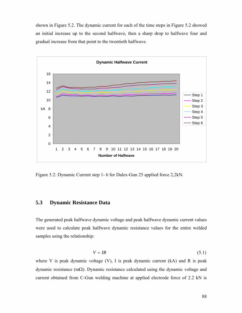
shown in Figure 5.2. The dynamic current for each of the time steps in Figure 5.2 showed

an initial increase up to the second halfwave, then a sharp drop to halfwave four and

radual increase from that point to the twentieth halfwave.

g

Dynamic Halfwave Current

0

2

4

6

8

10

12

14

16

1 2 3 4 5 6 7 8 9 10 11 12 13 14 15 16 17 18 19 20

Number of Halfwave

kA


Figure 5.2: Dynamic Current step 1- 6 for Dalex-Gun 25 applied force 2,2kN.

Dynamic Resistance Data

5.3

The generated peak halfwave dynamic voltage and peak halfwave dynamic current values

were used to calculate peak halfwave dynamic resistance values for the entire welded

samples using the relationship:

IRV = (5.1)

where V is peak dynamic voltage (V), I is peak dynamic current (kA) and R is peak

dynamic resistance (mΩ). Dynamic resistance calculated using the dynamic voltage and

current obtained from C-Gun welding machine at applied electrode force of 2.2 kN is

88

presented in Figure 5.3. Similar values obtained for the entire applied electrode force and

for all four welding machines used are presented in Appendix B.

Dynamic Resistance

0.08

0.16

0

0.02

0.04

0.06

1 2 3 4 5 6 7 8 9 10 11 12 13 14 15 16 17 18 19 20

Number of Halfwaves

0.1

0.12

0.14


Figure 5.3: C-Gun (2.2 kN) steps 1-6, Dynamic Resistance plot

)(mΩ

Figure 5.3 shows a common trend in the dynamic resistance behaviour of the welded

le ps 1 to

. The plots of each of the sample dynamic resistance graph showed an initial high

state effect of the material resistance and inter-contact resistance effect between the

samp s generated from the C-Gun welding machine, at 2.2 kN force, and time ste

6

dynamic resistance value at the first halfwave, followed by sudden sharp drop at about

the second halfwave and gradual increase in resistance from the second halfwave point to

a peak point and then a gradual decrease from the peak point. The initial high dynamic

resistance at the first halfwave is due to the effect of the contact resistance of the material,

this effect is not sustained and within the second halfwave with increase in heat generated

the contact resistance effect is overcome (102). The dynamic resistance due to the solid

89

welded material (plates) causes the dynamic resistance to increase to the peak point, with

a change of state from solid to a mixture of solid and liquid, the dynamic resistance drops

. This state accounts for the sudden change in dynamic resistance. The liquid state of

nward

trend of the dy ce curve (102).

It w bserv he o ance ves in endi

that the dynamic resistance curves of all the we ed sam av r tr d like the

ones in Figure 5.3, with some samples however showing some slight deviation. The slight

variation is expected because of som riability that may e ari rom the ma

or m e setti r inst t rea s etcet , 10).

It is observed that the peak points in the dynamic resistance curve of Figure .3 di

all at the halfw cycle e in all the time . Som f the ak p

are seen to be reached at earlier halfwave cycles times than thers. T e peak oint of t

dyn resista curve wel time s 4-6 rred bou he f

halfwave cycle (HW 4) an ing steps wav ycle

6). This can be explained as the effect of incr d wel urre t the gher

steps, such that the peak d ic resistance are hed the few cle t

com to the uced w g cu of steps 1-2 which takes r ha ave

5.4 Effective Weld Current (RMS) and Weld Diameter Dataset

The modelling of the resistance spot welding process parameters will require dynamic

resistance, effective weld current (RMS), weld diameter and applied electrode force.

Having determined dynamic resistance values for given applied electrode forces from the

previous section, this section presents effective weld current and weld diameter data

needed for the modelling process. Presented in Table 5.1 are effective weld current and

weld diameter dataset for C-Gun welding machine at an applied electrode force of 2.2kN.

(102)

the weld accounts for a decease in dynamic resistance as is noted with the dow

namic resistan

as o ed from t graphs f the dynamic resist cur

p h

shown

e simila

App x B,

ld le en

e va hav sen f chine

achin ngs o rumen ding era (3

5 d not

occur same ave tim steps e o pe oints

o h p he

amic nce s for ding step occu at a t t ourth

d ld we time 1-2 at about the sixth half e c (HW

ease ding c nt a hi time

ynam reac within first cy imes,

pared red eldin(94)

rrent longe lfw cycle

time to reach the peak points . This observation will be further discussed in modelling

section of Chapter 6.

90

Similar results were obtained for the entire samples welded. Figures 5.4 and 5.5 shows

the effective weld current (RMS) and weld diameter achieved for time steps 1 and 6.

Table 5.1: Additional Generated Data for Step 1 and 6, of C-Gun Machine at

2.2kN Force

Spec

imen

s.nr.

Fe (kN)

Is (kA)

dp (mm)

dpk (mm)

Mt (Nm)

Win. (Deg)

BA

Step

15-1 2.2 5.75 4.8 3.8 6.6 2.9 S Step 1 15-2 2.2 5.76 4.8 3.6 7.0 34.4 S Step 1 15-3 2.2 5.76 4.8 3.6 6.8 14.2 S Step 1 15-4 2.2 5.73 4.8 3.7 7.4 12.7 S Step 1 15-5 2.2 5.73 4.8 3.4 6.8 33.9 S Step 1 15-7 2.2 5.74 4.9 3.5 8.0 15 S Step 1 15-8 2.2 5.76 4.9 4 6.7 6.7 S Step 1

17-1 2.2 7.27 5.7 4.2 13.6 78.6 S Step 6 17-2 2.2 7.32 5.6 4.4 14.4 65.7 A Step 6 17-4 2.2 7.6 4.9 4 9.6 64.8 A Step 6 17-5 2.2 7.34 5.9 4.4 14.3 62 A Step 6 17-6 2.2 7.59 5 3.4 11.7 67.9 A Step 6 17-7 2.2 7.37 5.7 4 18.1 68.4 A Step 6 17-8 2.2 7.34 5.6 4.1 14.4 66.8 A Step 6

Abbreviation terms as used in the table are as follows: Fe: Electrode force (kN), Is:

Welding current (kA), dP: spot diameter with corona zone (mm), dpk: spot-diameter

(mm), BA: fracture type, A: plug failure, S: Interface fracture.

91

Effective Current

7.51375

5.7375

4

5

6

7

8

kA

0

1

2

3

1 6Time Steps

Current

Figure 5.4: C-Gun (2.2 kN) Average Values of Effective Weld Current for steps 1 and 6

Weld Diameter

5.55

3.65

0

1

2

3

4

5

6

1 6Time Steps

mm Weld Diameter

Figure 5.5: C-Gun (2.2 kN) Average Values of Weld Diameter for steps 1 and 6

92

The results of effective weld current and weld diameter in Figures 5.4 and 5.5 show that,

the average size of the achieved weld diameter is larger in samples made at time step 6

than time step 1. The increase in weld diameter from step 1 to step 6 is because of the

increase in current used from step 1 to step 6. Similarly, micrographs were obtained for a

umber of the samples welded. Presented in Figures 5.6 and 5.7 are micrographs of the n

nugget of some samples welded with Dalex PMS welding machine for step 1 and step 6

respectively.

Figure 5.6: Metallography of weld spot nuggets ple, Dalex PMS

igure 5.7: Metallography of weld spot nuggets of step 6, welded sample, Dalex PMS

of step 1, welded sam

F

93

These represent the two extremes of the time steps. The Figures show that the nugget

sizes produced in step six are bigger in size (Figure 5.7) than the nugget sizes from step

one (Figure 5.6). This agrees with the direct relationship between effective weld current

and achieved weld diameter.

The selection of the good weld quality range using weld diameter cut off value based on

Force

(kN)

Diameter

achieved

ctive

Current (kA)

Effective

Current

(kA)

Weld diameter

(mm)

xpulsion

Weld

Diameter

(mm)

observed expulsion limit is presented in Table 5.1.

Table 5.1: Observed Maximum Values: weld diameter, effective current and

observed expulsion weld diameter

Machine

Type

Applied

Electrode

Maximum.

Weld

Corresponding

Effe

Maximum Corresponding E

(mm)

2.2 5.9 7.34 7.51 5.6 5.6

2.6 6.1 8.32 8.41 6.0 None

C-Gun

None 3.0 6.2 8.62 8.66 6.1

2.2 5.6 7.41 7.43 5.3 None

2.6 6.0 8.39 8.39 6.0 None

DZ

3.0 6.6 9.39 9.42 6.2 None

2.2 6.60 8.33 8.58 6.15 5.8

2.6 6.50 8.76 8.84 6.2 None PMS

3.0 6.80 9.24 9.34 6.3 None

1.76 5.4 7.04 7.04 5.4 5.25

2.16 5.9 7.69 7.69 5.9 5.4

2.2 6.0 7.63 7.73 5.7 5.5

2.46 5.9 7.85 7.85 5.9 None

2.6 6.1 7.95 7.95 6.1 None

Dalex

3.0 6.3 8.55 8.57 5.9 None

94

In defining weld quality, weld diameter less than 3.7 mm was considered a bad weld

because it is below the stick limit. Theoretically, the weld diameter is expected to be

between 3.7mm and 4.7mm to be considered a satisfactory weld quality for the electrode

ear class used (19). Maximising the size of the weld diameter to a possible large size

efore expulsion point will give better weld quality (weld diameter).

ased on observation as shown in Table 5.1, weld diameter between 3.7 mm and less

an 5.25 mm was considered good weld. With less than 5.25 mm weld diameter as the

etter spot weld quality. Less than 5.25 mm weld diameter was taken as a cut-off point

ecause an expulsion was observed to occur at 5.25 mm during the welding process as

hown in the Table. This observation shows that there is no guarantee that expulsion will

ot occur at a weld diameter above 5.25 mm.

.5 Concluding Remarks

y using the equation (19)

w

b

B

th

b

b

s

n

5

tdt 54 <≤B , it was possible to have a guide to what defines

good or poor quality weld. The nugget sizes produced in step six are bigger in size than

e nugget sizes from step one because of higher current range applied. This agrees with

e direct relationship between effective weld current and achieved weld diameter.

ffective weld current achieved, in the time steps 6 are higher than in the steps one.

o expulsion was observed at below 5 mm weld diameter. This means that high chance

xist to push the current up to the point of producing this weld diameter without

xpulsion. The earliest expulsion was with Dalex 25 welding machine with a weld

iameter of 5.25 mm at an applied electrode force of 1.76 kN. Expulsions were frequent

s noticed at the lower applied electrode force than at higher applied electrode force. This

ay be because at the lower applied electrode force, larger gap exist between the plates

ontact surfaces which creates higher resistance. During the welding process with fast

eat generation mostly due to higher resistance and rapid growth of the nugget (23),

ithout adequate constraints chance for expulsion occurring will be very high.

a

th

th

E

N

e

e

d

a

m

c

h

w

95

The non linear nature of dynamic ables makes it difficult to use in

redicting weld quality. It is therefore important to model this variable in other to use it

r predicting weld quality.

resistance vari

p

fo

96

CHAPTER 6

MODELLING THE PROCESS PARAMETERS

6.1 Introduction

Presented in this Chapter are the models used for estimating the process parameters in the

sistance spot welding process. These process parameters are dynamic resistance,

applied electrode force, effective weld current and weld diameter. Dynamic resistance

generated from each welded sample showed non linear and complex behaviour in having

twenty halfwave dynamic resistance values per sample. An empirical model was

developed and used to curve fit the dynamic resistance curve, such that the twenty

halfwave dynamic resistance per sample was reduced to just one resistance value for each

sample welded. This estimated resistance per sample will be referred to as sample

resistance in this thesis. The level of error in the estimation was determined for each of

the samples using the root mean square error and sum of square criteria (103).

The prediction capability of the empirical model was improved by passing the outputs

from the model through neural network learning for intelligent and accurate prediction.

The predicted sample resistance from the neural network with applied electrode force and

effective weld current were used as in inputs in a second neural network model to predict

weld diameter.

our neural network types which are generalized feed forward, multilayer perceptron

ral network (RNN) types were

ained and tested to find the one with least error and best generalization capability, for

re

F

(MLP), radial basis function (RBF) and recurrent neu

tr

predicting sample resistance and the weld diameter. Such that for any desired weld

diameter it was possible to determine the optimum parameters that will be needed to

achieve the weld diameter.

97

6.2 Empirical Model for the Dynamic Resistance Parameter

hree

tages as is shown in Figure 6.1.

Dynamic Resistance Curve The first stage is the rly stage

eak point. The second stage is the peak point and the third stage is the dynamic

resistance from the peak point to welding completion.

6.2.1 First Stage

An empirical (mathematical) model that explains the pattern of the dynamic resistance

behaviour (102) was developed. The purpose was to use it to linearise the nonlinear

dynamic resistance curve and to be able to estimate a resistance value for each welded

sample. This is because a linear input parameter to the neural network model would help

improve the neural network prediction accuracy as discussed earlier in the literature

section. In developing this model the dynamic resistance curve was broken up into t

s

Figure 6.1: Trend Pattern of

ea of the resistance change from its initial value up to the

p

0 1 2 3 4 5 6 7 8 9 10 11 12 13 14 15 16 17 18 19 20

Number of Halfwaves

0.02

0.04

0.06

0.08

0.1

0.12

0.14

Dynamic Resistance Curve

First Stage Second

Stage Third Stage

R ) ( Ωm

98

Figure 6.1 shows that in e first few initial halfwave cycle times there is significant drop

in the

th

dynamic resistance followed by a gradual increase. Peak point is reached after few

me halfwave cycles depending on the welding current intensity (102). With the dynamic

resistance there is a corresponding increase in temperature and amount of energy

generated (23, 102). This is because resistivity increases with temperature. It ca be

concluded that changes in welding cycle time corresponds to changes in temperature and

generation of heat energy as the dynamic resistance progresses up to the peak point.

Based on observation of the dynamic resistance curve, it can be stated that the dynamic

resistance behaviour of the spot welded sample from the first halfwave cycle time t

peak point is directly related to the number of halfwave cycles plus the initial resistance

at first halfwave cycle time. Expressed mathematically:

ti

n

o the

01 RNR c +∝ .1)

(6

Such that

01 RNMR c +×= (6.2)

where 1R is a function that accounts for the resistance from first time cycle up to the

resistance at the peak point. cN is the number of half waves. 0R is the surface resistance

of the sample. Parameter M is a function of temperature which depends on the material

sist (94, 102), expressed by ance )( sR during current flow re

AlRs β= (6.3)

99

with β = specific electrical resistance (temperature dependant), l = length of current

flow in work piece and A = current area (electrode contact area). As is shown in Figure

6.2.

0.085 0.09

0.095

0.11

0.1 0.105

0.115

0.021 0.024 0.028 0.032 0.036 0.039 0.043 0.047 0.051 0.054 0.058 0.062 Input M

Relationship between Parameter M and Resistance

eter M on Resistance

The figure shows that increasing the input parameter

R)

1

( Ωm

Figure 6.2: Influence of Param

M generates an increase in the

value of the sample resistance . The effect of the initial resistance which is due to the

contact resistance between the surfaces of the welded plate in contact disappears after the

first few welding halfwave cycles. This agrees with Matsuyama (24) findings in which he

concluded that the resistance due to the interface contact resistance is not very important

in normal resistance spot welding. 6.2.2 Second Stage

This peak point is

)(R

The second phase is the peak point of the dynamic resistance curve.

referred to by most researchers as the β peak (94, 102). In explaining the formation of the

β peak, De et al (94) in reviewing the work by Dickinson (102) in this area mentioned that

100

at the peak point there is decreased interface resistance which is influenced by the

increased bulk resistivity with temperature. This eventually leads to an overall decrease in

the sample resistance away from the peak point (94), such that the peak point stands out.

his view is consistent with the views of other researchers (102). However, at this T β peak

there is no change in dynamic resistance and welding cycle time hence:

0=CdN

dR

With the change in dynamic resistance to the change in welding cycle time being equal to

zero 0dR at th β peak it is possible to estimate the parameter M=CdN

is . The parameter

M in equation (6.2) is determined by taking the second order partial derivative of the

same equation (6.2).

6.2.3 Third Stage

The third phase corresponds to the downward slope from the β peak of the dynamic

ure 6.3. resistance curve, Fig

Figure 6.3: Dynamic resistance trend from the peak point downwards

Slightly away from the β peak is a marked decrease in dynamic resistance sloping

downwards as the welding cycle time progresses. The drop in dynamic resistance is due

Dynamic Resistance

0.12

0.124

0.128

0.132

Ωm

1 2 3 4 5 6 7 8

Halfwave Cycle Time

101

to a change in contact diameter (contact resistance) because of the change of state from

solid to liquid of the sheet surfaces in contact and increase in the cross sectional area (23,

94).

Estimating the change in cross sectional area of the contact surfaces is difficult because

the contact diameter is not constant during welding (23), Matsuyama (23) used simulation

method to determine contact diameter but only at a particular time (t). Contact diameter

change at plate interface (23) during the welding process is dependent on time. The

change in cross sectional area (contact diameter) affects the downward slope of the curve

from the β peak (102).

rve from the The downward slope of the dynamic resistance cu β peak is observed to

llow a mathematical function of inverse relationship between the dynamic resistance

ownward slope

fo

d ( 2R ) and the welding cycle time ( ) raised to power index “n” ( n is

0 and 1) and strongly influences the downward slope from

the

Nc

an index that ranges between

β peak .

Represented thus:

(6.4)

Such that,

n

cNR ∝2

ncN

KR =2 (6.5)

here 2R is the dynamic resistance of the downward slope from the β peak, is the cNW

welding cycle time, n is power index and K is a constant. The power index n describes

the steepness of the slope. The physical cause of the downward slope is due to drop in

interface resistance as a result of change of state from solid to liquid as the faying surface

elts (104). K directly influences the sample resistance. Increasing K leads to an increase

esistance as is shown in Figure 6.4.

m

in sample r

102

Figure 6.4: Influence of Parameter K on Resistance

t describes the dynamic resistance will then be the total of

6.2.4 Total Resistance

The mathematical function tha

1R and 2R acting in parallel, such that

21

111RRR

+= (6.6)

R is total resistance; 1R and 2R are defined earlier.

Substituting equations (6.2) and (6.5) into equation (6.6), the expression becomes;

KN

RNMR

nc

c

++×

=)(

11

0

(6.7)

such that,

Relationship between Parameter K and Resistance

0 0.02 0.04

0.1 0.12 0.14

0.359 0.388 0.416 0.444 0.472 0.500 0.529 0.557 0.585 0.613 0.641 0.670 Input K

Output R

0.06 0.08 2

( Ωm )

103

)())()((1

0

0

RNMKRNMNK

R c

cn

c

+×+××+

= (6.8)

By making R the subject of the equation;

))()((( RoNcNcMNcKRoKNcMKR nn ×+××+

×+××= (6.9)

and are known for each sample welded, 0R cN K and M can be estimated. To determine

the unknown parameter (power index), the effect of change of on the slope of the

dynamic resistance curve was evaluated by taking values from 0 to 1 and substituting

see the effect on the model. By increasing n

0.2, the drop in resistance is noticeable but far from actually fitting the dynamic

n n

n

into a plot of equation 6.9.

The value of n is incrementally increased to

to

resistance curve. Further increasing n to 0.5 correctly fits the curve as is shown in Figure

6.5.

104

igure 6.5: Curve fitted Model at n = 0.5

The power index n was taken as 0.5 in this model due to best fit. It is observed that the

dynamic resistance curve fitting model responds to this power index n by some unknown

non linear relationship function. This relationship is assumed to be depending on the

contact area of the sheet surfaces during the welding process (23).

o calculate sample resistance R, the parameters K and M have to be determined. M and

taking partial derivatives of equation (6.7) at the

F

T

N can be estimated by β peak where

0=cdN

dR , such that;

2 4 6 8 10 12 14 16 18 20 0.065

0.07

0.075

0.08

0.085

0.09

0.095

0.1

0.105

0.11

0.115

Halfwave Cycle Time

Dynamic Resistance Fitted

Curve Fitted Model

Ωm

105

nKNRNMM

dNdRR n

c

c

)1(20

2 ))/(()/1( −++×−=

− (6.10)

nKNRNM

MR

dNdR n

c

c

)1(202 )( −−+×

= (6.11)

aximum a

t 0=cdN

dR , when pc NN = , pN is the cycle number at βM peak

MnRNMN

K

RNMnNK

pn

p

pp

×

+××=

+×−×

− 20

)1(

20

)(

))(1(

The equation will be

Mn

M

×=

1

RNMM

KnN

KnNRNM

p

np

npp

+×=

×

=×

−+×

−

−

20

)1(

)1(20

)(

0)(

pN

Similarly parameter M will be

pK 0 )(2= (6.12)

RNM 2+×

106

p

p

NRNK

2)2( 0

2 −=M (6.13)

Such that once parameter M is estimated K can be determined and vice versa. The total

resistance (R) can therefore be determined by the equation:

5.005.1

0

)( cc

c NRNMK

RNMKR ×+

×++××

= (6.14)

his equation is the model that can be used for curve fitting the dynamic resistance curve

nd for determining the sample resistance , once the parameters

T

)(R K and Ma are

stimated. This model equation (6.14) was used to test one hundred and seventy samples

er machine for all four machines used. This was to confirm the model suitability for

urve fitting the dynamic resistance curves and for estimating the resistance of welded

amples.

he curve fitting and estimation of the unknown parameters were done for each welded

ample in MATLAB (105). This was done by first making a plot of the dynamic resistance

curve in MATLAB, followed by the equation (6.14) of the model being written in the

MATLAB curve fitting custom solution option (105). The confidence interval was set at

95%. Initial parameter values were assumed and supplied (103) before starting iteration

process for determining the final value of the parameters. Assuming initial parameter

values were because the iteration process can not proceed without some initial values

supplied. These initial values were randomly generated in MATLAB, and the correct

parameter values were determined through the iteration process (103).

Through the iterative process the

e

p

c

s

T

s

K and M parameters which curve fitted (best fits) the

dynamic resistance curve were determ ith the parameters ined. W K and M known it was

107

possible to determine the sample resistance for each of the welded samples. This was

done by substituting the values of the parameters K and M generated, and which is

the initial dynamic resistance value into the model expression of equation (6.14).

Presented in Figure 6.6 is the result of the curve fitting of the dynami rve

for one of the samples taken from DZ machine under applied electrode force of 3.0 kN,

using the model (equation 6.14) to make the fit.

oR

c resistance cu

108

4 10 1 16

109

sis urve

Sim esults w obtain ll lded s . Pres in Appendix C are the

results of the curve fit o sa take all elding in

different applied electrode force.

6.3 pplyi he Em al el

The primary purpose of the empirical mode tion 6.14) was to lineari

inc t no ar dy esi param ddi , the is

exp for est ing sam sista an u wel onditio

Figure 6.6: Fitted Dynamic Re tance C : DZ machine at 3.0 kN Force.

ilar r ere ed for a the we amples ented

f some mples n from four w mach es, for

A ng t piric Mod

l (equa se the

onsisten nline namic r stance eter. A tionally model being

lored imat ple re nce in nknown ding c n.

2 6 8 12 4 18 20

0.07

0.075

0.08

0.085

0.09

0.095

0.1

0.105 Dynami tance c Resis

Fitted

Ωm

Model Fitted Dynamic Resistance Curve

H Cycle

alfwave Time

Th irical l is ap lied by determinin the param terse emp mode p g e K , M and and

substituting these values into the mo uation mate le resis Th

of square error and root m r in each of the sam t

were determine ). In all the case um of square erro oot me ar

we ifican ss tha 103) show d es n. Pre in

6.1 are the

oR

del eq to esti samp tance. e sum

ean square erro ple resis ance estimated

d (103 s the s r and r an squ e error

re sign tly le n one ( . This s a goo timatio sented Table

K , M and v det d for mples welded in C-Gun m

which were used to determ sam sist

Table 6.1: Estim samp tan ECurrent

Weld Di

(mm)

K SuSqu

RM Ro ( R

oR alues ermine some sa achine

ine the ple re ance (R).

ated le resis ce (R) ffective

(kA) ameter

M

m of ares

SE

Ω ) m

( Ωm )

6.48 3 .7 0.5391 0.029 0.001 0.008 0.106 0.101 6.48 3 0..7 6395 0.021 0.0002 0.004 0.085 0.11 6.52 3 .7 0.5928 0.022 0.0005 0.005 0.091 0.104 6.5 3 .7 0.5886 0.023 0.0005 0.005 0.092 0.105 6.53 3.9 0.5961 0.021 0.0003 0.004 0.086 0.105 6.52 3.7 0.5845 0.023 0.0004 0.005 0.089 0.104 6.52 3.7 0.5942 0.022 0.0005 0.005 0.091 0.105 6.51 3 .7 0.6391 0.019 0.0004 0.004 0.086 0.108 6.99 4 0.5125 0.029 0.0004 0.005 0.093 0.097 7.01 4 0.5598 0.024 0.0526 0.054 0.087 0.102 6.99 4 0.5394 0.024 0.0529 0.054 0.085 0.099 6.97 4 0.5507 0.025 0.0003 0.004 0.086 0.101 6.93 4 0.5823 0.024 0.0002 0.004 0.085 0.105 6.96 4 5394 0.026 0.0003 0.004 0.083 0.1 0.6.97 .5164 0.025 0.1194 0.081 0.089 0.096 4 0

7 4 0.5598 0.024 0.0005 0.006 0.092 0.102 7.35 4 0.5536 0.027 0.0002 0.003 0.082 0.102 7.34 4.4 0.5164 0.031 0.0002 0.004 0.089 0.099 7.36 4.4 0.5132 0.029 0.0002 0.004 0.087 0.097 7.33 4.3 0.537 0.027 0.0002 0.003 0.083 0.1 7.28 4.5 0.5536 0.031 0.0632 0.059 0.084 0.105 7.31 4.5 0.0002 0.003 0.085 0.104 0.5628 0.027 7.36 4.5 0.5281 0.028 0.0002 0.003 0.082 0.099 7.39 4.5 0.5267 0.028 0.0002 0.003 0.083 0.099 7.71 5.7 0.5334 0.03 0.0001 0.002 0.081 0.101

Effective Current

Weld Diameter

K

M

Sum of Squares

RMSE

Ro (

R (Ωm ) Ωm )

110

(kA) (mm)

7.74 5.5 0.5123 0.032 0.0001 0.003 0.085 0.098 7.7 5.5 0.4893 0.035 0.0564 0.056 0.083 0.096 7.7 5.6 0.5003 0.033 0.0577 0.057 0.082 0.097 7.75 5.6 0.489 0.035 0.0002 0.003 0.086 0.096 7.73 5.6 0.4893 0.035 0.0002 0.003 0.088 0.096 7.73 5.5 0.489 0.035 0.0003 0.004 0.091 0.096 7.76 5.5 0.5003 0.033 0.0002 0.003 0.085 0.097 8.18 6 0.4944 0.036 9.80E-05 0.002 0.083 0.097 8.2 5.9 0.4709 0.042 0.0490 0.052 0.084 0.094 8.14 5.9 0.4721 0.039 0.0001 0.002 0.084 0.094 8.15 5.9 0.4702 0.039 8.68E-05 0.002 0.084 0.093 8.13 5.9 0.46 0.036 0.1166 0.08 0.084 0.091 8.12 5.8 0.4709 0.04 8.08E-05 0.002 0.084 0.094 8.16 6 0.4552 0.042 0.0001 0.003 0.086 0.092 8.18 6 0.46 0.041 0.0001 0.002 0.084 0.092 8.59 6 0.4348 0.042 0.0001 0.003 079 0.088 0.8.62 6 0.4128 0.046 0.0001 0.002 0.081 0.084 8.61 5.9 0.4186 0.046 9.16E-05 0.002 0.081 0.085 8.6 5.6 0.4358 0.046 0.0028 0.013 0.08 0.089 8.66 6.1 0.4095 0.045 9.56E-05 0.002 0.083 0.084 8.63 6 0.4186 0.042 0.0415 0.048 0.079 0.085 8.62 6.2 .4256 0.043 9.66E-05 0.002 0.079 0.080 6 8.59 6.2 0.4358 0.04 6.81E-05 0.002 0.081 0.088 3

pirical model to estimate sample

As is shown in Table 6.1, it is possible to use the em

resistance once K and M parameters are determined through an iteration process and

oR known.

e parameters are plotted and used for estimation needed values of

To predict sample resistance R without going through an iteration process, graphs of

M and K values of th

and oR for a desired weld diameter. Presented in Figure 6.7 is a plot of the parameters

M and K of one of the welding machines.

111

Figure 6.7: Machine C-Zange – Parameters M and K and Applied electrode force 2.2KN

To test if this is able to estimate sample resistance.

The parameters are estimated from the graph of Figures 6.7 at a desired weld diameter of

.3 mm. The values for 5 M and K were determined from the graph as K = 0.6561, M =

0.02623. Initial dynamic resistance at first halfwave for this welding machine

average is 0.094448.

Substituting these values into the model equation (6.13);

Ro

)))5.0^(*())5.1^*(/(())*(*( NcRoNcMKRoNcMKR +++=

R = (0.6561*(0.02623*20+0.007563))/((0.6561+(0.02623*20^1.5))+(0.007563*(20^0.5)))

R = 0.101 To validate the above estimate, this value was compared to the actual value of the

dynamic resistance at weld diameter of 5.3 mm for this machine and applied electrode

force. Four values of sample resistance (R) were obtained. The values were 0.116201,

Ωm

112

0.115402, 0.115902 and 0.112434. Percentage accuracy in estimating was 85%, 86%,

85.5% and 88.9% respectively.

Similarly compared for weld diameters of 5.9 mm, the parameters were estimated from

the graphs of Figures 6.7, the value of R obtained was 0.1013 Ωm . Compared to actual

value of R which was 0.10126 Ωm , a percentage accuracy of 99.98%. This was done for

all the samples and the accuracies were all above 85%.

The applicability of this model was further verified to any of the welding machines

without an identifier using data set generated from all the welding machines. The essence

of this was to see how the graph can be used to accurately estimate sample resistance for

a desired weld diameter in an unknown situation (unknown machine). Graphs were

developed using the data generated from the model expression for different weld

diameters. Presented in Figure 6.8 and 6.9 are the plots of K , M and parameter

values for different weld diameters for a number of samples welded at different applied

electrode force using the four welding machines. These parameters were used for

estimating sample resistance for a desired weld diameter in unknown welding machines.

oR

113

Generated K and M parameters

Figure 6.8: Parameters K and M Generated

114

)( Ωm

Generated Parameter R0

Figure 6.9: Parameter oR Generated

The obtained result of the sample resistance was compared with the actual values of

sample resistance obtained. Presented in Figure 6.10 is the estimation of sample

resistance for samples welded in an unknown welding machine.

115

Actual Resistance to Predicted

0.2

0.02

0.04

0.06

0.08

0.1

0.12

0.14

0.18

R0.16

Actual R

Predicte

Figure 6.10: Predicted Resistance to actual in Dalex Machine

The Figure shows the actual resistance compared to the predicted. The predicted is not

following the actual. Similar estimations were made without identifying (unknown) the

ence (error) of the predicted to the actual ranged

between 16% to 149%. The large prediction error as is shown in figure 6.10 may be

because the model can only track linear changes and is not able to follow nonlinear

d changes in new situation. Statistical analysis will be carried out to

d t e relationships betwee p rameters. If nonlinear relationships are

c n t between the param nd the samp resistan then neu l networ

techniques will be the most appropriate method to use in modelling the process.

welding machines. The percentage differ

ynamic and complex

e ermine th n the a

o firmed to exis eters a le ce ra k

0 1 2 3 4 5 6 7 8 9 10 11 12 13

Number of samples

d R

Ωm

116

T ror was investigated by carrying out correlation analysis and multiple

regression analyses between the p an e re e R ted le

6.2 is the correlation of the parameters to one another.

Table 6.2: Correlations Matrix Current

(kA) eld

) M

he cause of this er

arameters d sampl sistanc . Presen in Tab

W Diameter(mm

K Ro R

Current (kA) 1.000 Weld Diameter 0.951 1.000

(mm) K -0.943 -0.884 1.000 M 0.959 0.921 -

0.956 1.000

Ro ( Ωm ) -0.648 -0.569 0.457 -0.479 1.000 R ( Ωm ) -0.912 -0.830 0.979 -0.922 0.466 1.000

The table shows significant linear correlation between the parameters. Strong linear

correlation exists between current and all the parameters and between weld diameter and

all the parameters with slight reduction with Ro. The linear correlation coefficient

between the parameters K, M and Ro are about 0.5 and are considered significant. The

rediction error is therefore not due to lack of linear correlation between the parameters. p

Further investigation was done using multiple linear regression analysis to ascertain the

relationship between the predicted variable R (sample resistance) to the other variables.

Presented in Table 6.3 is the result of the multiple regression for sample resistance (R).

Table 6.3: Multiple Correlations Matrix

Results of multiple regression for R ( Ωm ) Summary measures Multiple R 0.9840 R-Square 0.9683 Adj R-Square 0.9645 StErr. of Est. 0.0012 ANOVA Table Source df SS MS F p-value Explained 5 0.0020 0.0004 256.6746 0.0000 Unexplained 42 0.0001 0.0000 Regression

117

coefficients

Coeffici t Std Err t-value p-value limitenLower Upper

limit Constant 0.0146 0.0215 0.6797 0.5004 -0.0287 0.0579 Current (kA) 0.0001 0.0019 0.0759 0.9399 -0.0038 0.0041 Weld Diameter (mm) 0.0014 0.0007 2.1295 0.0391 0.0001 0.0027 K 0.1279 0.0124 10.2839 0.0000 0.1028 0.1531 M 0.0146 0.1090 0.1336 0.8944 -0.2055 0.2346 Ro 0.0996 0.0757 1.3159 0.1954 -0.0531 0.2523

The R-Square, adjusted R-Square, high F value and low standard error shows good

stimation accuracy. The p-value gives indication of clear linear relationship existing

nly between the sample resistance (R) and weld diameter, K and Ro. While the

icated by

e high p value. The relationships were combinations of linear and non linear

R and some of the parameters. To improve the

rediction accuracy neural network technique will be employed to learn the pattern in the

(known), without the need to conduct the welding experiment or going through the

e

o

relationship between R and current and M parameter are not seen as linear as ind

th

relationships among the parameters. The level of estimation error in the result obtained

by using the graph suggests that the technique is not appropriate for an accurate result.

The values were further linearised using logarithm function (89) but the improvement in

estimation accuracy was little.

It can be concluded that the sample resistance of a desired weld diameter in an unknown

welding machines can be predicted using the graphs. This is however with high level of

prediction inaccuracy mostly because of the nonlinear and complex relationship that

exists between the sample resistance

p

data and to be able to make accurate prediction (6).

6.4 Improving the Empirical Model using Artificial Neural Networks

The generated parameters from the empirical model were passed through neural network

learning in other to improve the prediction accuracy. Such that for any desired weld

diameter in any of the welding machines the sample resistance will be determined

118

iteration process of determining the parameters K , M and oR . The inputs are weld

diameter and parameters K , M and oR . Sample resistance was the output. The result

was validated (tested) and further cross validated on dataset not used for the training and

then used to make prediction on dataset not seen before.

Four neural network types which are generalized feed forward, multilayer perceptron

(MLP), recurrent network and radial basis function (RBF) were tested to find the best

predictor to be used for improving the empirical model.

6.4.1 Training using Generalized feed forward neural network

co ections

an jump over one or more layers (33). The inputs for this network as mentioned earlier are

le resistance

from the empirical model is the output.

The dataset were randomised to achieve even spread. Then the columns were tagged as

inputs and outputs. 70% of the data set (exemplars) was set apart (tagged) for training,

15% for training and another 15% for cross validation. 20 exemplars were kept as

production data for production testing.

The generalized feed forward network design was made up of 2 inputs processing

elements, 1 output processing element, 502 exemplars, 3 hidden layers, with first hidden

layer made up of 16 processing elements, TanhAxon transfer function, with momentum

learning rule. The second hidden layer was made up 8 processing elements, TanhAxon

transfer function and momentum learning rule. The third hidden layer was made up of 5

processing elements, TanhAxon transfer function and momentum learning rule also. The

outer layer consists of one processing element, BiasAxon transfer function and

conjugated gradient learning rule. 3000 epochs were specified for the training iterations.

Generalized feedforward networks are a generalization of the MLP such that nn

c

desired weld diameter and applied electrode force, while linearised samp

119

The generated architecture design showing input and out put files with the hidden layers

and transfer functions is presented in Figure 6.11.

Figure 6.11: Generated generalized feedforward network architecture design (106)

The results of the training and cross validation are presented in Figure 6.12.

Mean Square Error versus

0 0.1 0.2 0.3 0.4 0.5 0.6

1 200 399 598 797 996 1195 1394 1593 1792 1991

Epoc

Training

Cross Validation

MSE

Figure 6.12: Training performance of the generalized feedforward network

120

The result of the training performance shows a good performance and a small error of

about 0.05 at training epochs of 2000. The training was therefore stopped at 2000 epochs.

The mean square error MSE curve showed a downward slope (weight decay) indicative

of good performance. The network was tested to validate the consistency of the

performance.

The testing error is measured by the linear correlation coefficient (r), mean absolute error

(MAE), normalised mean squared error (NMSE) and mean squared error (MSE). These

statistical parameters give an acceptable measure of the level of control and performance

quality of the network (93). How closely the predicted resistance lines are following the

ctual resistance was determined as is shown in Figure 6.13.

Figure 6.13: Testing performance of the generalized feedforward network.

a

Predicted Resistance to Actual

0

0.05

0.1

0.15

0.2

0.25

1 1 1 3 1 71 91

Exemplar

1 2 1 4 51 61 81 101

R Actual

R Predicted

Ωm

121

The result of the testing performance gave a mean sum of squares of 0.001, and mean

absolute error (MAE) of 0.03. This indicates a good performance. The normalised mean

quared error (NMSE) was about 0.83 and the linear correlation coefficient was 0.52. A

linear correlation coefficient of 0.52 shows that the set of point are not close to a straight

line, which indicates a poor correlation. The graph in Figures 6.13 shows that estimated

resistance is not closely following the actual resistance value. The performance of the

network will be further validated by presenting data not seen before by the network to see

how well it can generalize. Table 6.4 shows the predicted resistance (R) to the estimated

resistance, and the estimation accuracy using the generalized feedforward neural network

type.

Table 6.4: Predicted Resistance to Actual Resistance using generalized feedforward

Neural Network type.

Machine Type

Applied Force (kN)

Weld diameter

(mm)

R predicted mΩ

R actual mΩ

Difference

% Difference

s

PMS 3 3.7 0.1186 0.1079 0.0107 9.9222 C-Gun 3 4.4 0.117 0.1662 -0.049 -29.591 Dalex-35 3 4 0.1191 0.089 0.03 33.741 Dalex-25 2.46 5.7 0.0986 0.0716 0.0271 37.799 Dalex-35 3 4 0.1191 0.1017 0.0174 17.116 PMS 2.2 5.3 0.0959 0.1154 -0.019 -16.88 Dalex-25 2.46 4 0.1123 0.0739 0.0384 51.949 Dalex-25 3 3.7 0.1186 0.1015 0.0171 16.892 C-Gun 2.2 4.4 0.1063 0.1178 -0.012 -9.8047 Dalex-25 2.46 3.6 0.1115 0.084 0.0275 32.693 Dalex-25 2.46 5.5 0.0991 0.0714 0.0277 38.754 C-Gun 2.2 3.5 0.1087 0.1053 0.0035 3.3057 Dalex-25 2.46 3.8 0.1124 0.0828 0.0295 35.67 Dalex-35 3 6.3 0.1079 0.1378 -0.03 -21.708 Dalex-25 2.16 5.4 0.1001 0.0578 0.0423 73.055 C-Gun 3 6.5 0.1103 0.1408 -0.031 -21.665 Dalex-25 2.46 3.6 0.1115 0.0889 0.0226 25.467 PMS 2.6 3.8 0.1167 0.1262 -0.009 -7.5071 Dalex-25 1.76 4 0.1034 0.0966 0.0068 7.0807

Table 6.4 shows marked differences between the predicted resistances to the actual, with

prediction error of about 3% to 73%. The prediction output of this network using real

122

data not used for training the network is presented in Figure 6.14. This is to further

evaluate how well the network is able to generalize.


0

0.05

0.1

0.15

0.2

1 3 5 7 9 11 13 15 17 19 21

Exemplar

R predicted

R actual mΩ

igure 6.14: Validation performance of the generalized feedforward network. F

The graph showed that the generalisation is very poor. The network was not able to

predict accurate output for data that it has not seen before. Though a large error of 3% to

73%, it is an improvement from the earlier estimation error of about 16% to 149%. To

achieve reliable and usable process model this error is considered high and unacceptable.

Other neural network types will be tested.

6.4.2 Training using Multilayer Perceptron neural network type

Multilayer perceptrons (MLP) are layered feedforward networks architecture which is

pically trained with static backpropagation (33). In this network architecture there are 2

output

processing elements (linearised sample resistance), 487 exemplars and 1 hidden layer.

ty

input processing elements (desired weld diameter and applied electrode force), 1

123

The hidden layer has 16 processing elements, TanhAxon transfer function with

momentum learning rule. The output layer uses BiasAxon transfer function with

conjugate gradient learning rule. The hidden layer and the process elements were

determined by trial and error and by comparing the error output. The generated network

architecture is shown in Figure 6.15.

Figure 6.15: Generated multilayer perceptrons (MLP) network architecture design (106)

The levels of errors for the training and cross validation are shown in Figures 6.16.

Mean Square Error versus Epoch

0

0.01

0.02

0.03

0.04

0.05

0.06

0.07

0.08

0.09

0.1

1 300 599 898 1197 1496 1795 2094 2393 2692 2991

Epoch

MSE Training MSECross Validation MSE

Figure 6.16: Training performance of the multilayer perceptrons (MLP) network

124

Similar to the generalised feedforward neural network type, the result of the training

performance of the multilayer neural network showed good performance with an error

output of about 0.05 at training epochs of 3000 and cross validation error of 0.06 at same

epoch of 3000. The downward slope (weight decay) however did not indicate a good

training and cross validation performance, as the slope did not show a significant drop.

The overall network performance was confirmed by the testing performance result. The

sting performance of the multilayer perceptron neural network used is presented in

perceptrons (MLP) network.

The test performance result gave a mean sum of squares of 0.008, mean absolute error

(MAE) of 0.02 indicating good performance. Normalised mean squared error (NMSE) of

te

Figure 6.17.


0

0.05

0.1

0.15

0.2

0.25

R ActuaR l

R Pred

1 11 21 31 41 51 61 71 81 91 101

Exemplar

ictedΩm

Figure 6.17: Testing performance of the multilayer

125

0.67 and linear correlation coefficient of 0.6. In the graph of Figure 6.17, the estimated

resistance is not closely following the actual resistance value, it is however performing

better than the feedforward neural network type. The performance of the network will be

validated using data set not seen before by the multilayer perceptron neural network.

Table 6.5 shows the predicted resistance (R) to the estimated resistance, and the

estimation accuracy using the multilayer perceptron neural network type.

Table 6.5: Predicted Resistance to Actual Resistance using multilayer perceptron

neural network type.

Machine Type

Applied

Force (kN)

Weld diameter

(mm)

R predicted (mΩ)

R actual (mΩ)

Difference

% Difference

PMS 3 3.7 0.1134 0.1079 0.0055 5.1089 C-Gun 3 4.4 0.1212 0.1662 -0.045 -27.09 Dalex-35 3 4 0.1175 0.089 0.0285 32.023 Dalex-25 2.46 5.7 0.0766 0.0716 0.005 7.0184 Dalex-35 15.612 3 4 0.1175 0.1017 0.0159 PMS 2.2 5.3 0.0837 0.1154 -0.0317 -27.446 Dalex-25 2.46 4 0.0951 0.0739 0.0212 28.619 Dalex-25 3 3.7 0.1134 0.1015 0.0119 11.773 C-Gun 2.2 4.4 0.1042 0.1178 -0.0136 -11.527 Dalex-25 2.46 3.6 0.0877 0.084 0.0037 4.3658 Dalex-25 2.46 5.5 0.0758 0.0714 0.0044 6.1602 C-Gun 2.2 3.5 0.0998 0.1053 -0.0054 -5.1532 Dalex-25 2.46 3.8 0.0918 0.0828 0.009 10.833 Dalex-35 3 6.3 0.1077 0.1378 -0.0301 -21.858 Dalex-25 2.16 5.4 0.096 0.0578 0.0381 65.951 C-Gun 3 6.5 0.1129 0.1408 -0.0279 -19.828 Dalex-25 2.46 3.6 0.0877 0.0889 -0.0012 -1.3175 PMS 2.6 3.8 0.1229 0.1262 -0.0033 -2.6032 Dalex-25 1.76 4 0.0978 0.0966 0.0012 1.285

Table 6.5 shows a prediction error of 1% to 65% using real data not used for training the

network. This generalization is presented in graph form in Figure 6.18. The graph showed

that the generalisation is slightly improved from the generalized feedforward neural

etwork type. It is still considered generally poor. n

126


0.2

0

0.05

0.1

0.15

1 3 5 7 9 11 13 15 17 19 21

Exemplar

R predicted

R actual mΩ

Figure 6.18: Validation performance of the multilayer perceptrons (MLP) network

Redial basis neural network type and Recurrent neural network were explored to see if

there will be further improvement in the prediction of sample resistance.

6.4.3 Training with Redial Basis Function Neural Network

Radial basis function (RBF) networks are nonlinear hybrid networks typically containing

a single hidden layer of processing elements (PEs). This layer uses gaussian transfer

functions. The centres and widths of the gaussians are set by unsupervised learning rules,

and supervised learning is applied to the output layer. These networks tend to learn much

faster than MLPs (33).

ork architecture design to be used here is made up of 2

with no

The radial basis function netw

input processing element with 1 output processing element, 487 exemplars,

127

hidden layer, 10 cluster centres, using consciencefull competitive learning with Euclidean

metrics (92). The output layer uses the conjugate gradient learning rule and Bias Axon

transfer function. 100 epochs of iteration is done for the unsupervised learning with a set

rate of decay and 1000 epochs for the supervised learning. The generated network

architecture design is shown in Figure 6.19.

Figure 6.19: Generated Radial basis function (RBF) network architecture design (106)

This Radial basis function network architecture was trained and cross validated. The

result of the training performance and cross validation is shown in Figure 6.20.


0.04

0

0.02

1 100 199 298 397 496 595 694 793 892 991

Epoch

0.06

0.08

0.1

0.12


Figure 6.20: Training performance of the Radial basis function (RBF) network

128

The Radial basis function training performance result shows a mean square error output

of about 0.07 at a training epoch of 180 and cross validation error of 0.09 at an epoch of

17. The downward slope (weight decay) did not indicate a good training and cross

e of the

nction network was further validated by testing its

performance. The result of the test perform

1

validation performance. The network will be tested to confirm overall performanc

network. The Radial basis fu

ance is presented in Figure 6.21.

Predicted Re to Acsistance tual

0.05

0.1

0.15

0.2

0.25

R R ActualR Predicted

01 11 21 31 41 51 61 71 81 91 101

Exemplar

)(mΩ

Figure 6.21: Testing performance of the Radial basis function network

The test performance result is poor. Though with a good mean sum of squares of 0.001,

and mean absolute error (MAE) of 0.02. The performance is not consistent as the

normalised mean squared error (NMSE) was 0.98 and linear correlation coefficient was

0.24. The graph (Figure 6.21) shows the estimated resistance is not closely following the

actual resistance value at all. The performance of the network validated using data set not

129

seen before by the Radial basis function neural network is presented in Table 6.6 and

Figures 6.22 respectively.

Table 6.6: Predicted Resistance to Actual Resistance using Radial basis function


Machine Type

Applied

Force (kN)

Weld diameter

(mm)

R predicted mΩ

R actual mΩ

Difference

% Difference

PMS 3 3.7 0.1174 0.1079 0.0095 8.8182 C-Gun 3 4.4 0.1156 0.1662 -0.0506 -30.429 Dalex-35 3 4 0.1175 0.089 0.0285 32.024 Dalex-25 2.46 5.7 0.0945 0.0716 0.023 32.088 Dalex-35 3 4 0.1175 0.1017 0.0159 15.612 PMS 2.2 5.3 0.1037 0.1154 -0.0117 -10.143 Dalex-25 2.46 4 0.1215 0.0739 0.0475 64.314 Dalex-25 3 3.7 0.1174 0.1015 0.016 15.718 C-Gun 2.2 4.4 0.116 0.1178 -0.0018 -1.4936 Dalex-25 2.46 3.6 0.1089 0.084 0.0249 29.596 Dalex-25 2.46 5.5 0.0899 0.0714 0.0184 25.808 C-Gun 2.2 3.5 0.1161 0.1053 0.0109 10.34 Dalex-25 2.46 3.8 0.1152 0.0828 0.0324 39.089 Dalex-35 3 6.3 0.1037 0.1378 -0.0341 -24.738 Dalex-25 2.16 5.4 0.1045 0.0578 0.0466 80.637 C-Gun 3 6.5 0.1029 0.1408 -0.0379 -26.924 Dalex-25 2.46 3.6 0.1089 0.0889 0.02 22.539 PMS 2.6 3.8 0.1171 0.1262 -0.0091 -7.2037 Dalex-25 1.76 4 0.1186 0.0966 0.022 22.776

The table shows the predicted resistance (R) to the estimated resistance, and the

estimation accuracy. Table 6.6 shows a prediction error of about 1.5% to 80% using real

data not used for training the network. The graph of Figure 6.22 shows that the

generalisation is poor, as the predicted resistance is not following the actual resistance.

130

6.4.4 Training with Recurrent Network

Recurrent neural networks was used for training the data set and for predicting output.

Recurrent neural networks can have an infinite memory depth (33) and thus find

relationships through time as well as through the instantaneous input space (33). Most real-

world data contains information in its time structure. Recurrent networks are the state of

the art in nonlinear time series prediction, system identification, and temporal pattern

classification (33). Though the set of data presented to the network is not a typical time

series prediction dataset, it is however a time dependent variable event.

The recurrent network architecture used here is made up of 2 input processing elements

with 1 output processing element as in other earlier architectures used. There are 480

exemplars, with 1 hidden layer and an input layer Axon. There are 16 processing

lements in the hidden layer and uses TanhAxon transfer function and momentum


0

0.05

0.1

0.15

0.2

1 3 5 7 9 11 13 15 17 19 21

Exemplar

mΩ

R predicted

R actual

Figure 6.22: Validation performance of the Radial basis function (RBF) network

e

learning rule. The output layer consists of BiasAxion Transfer function and conjugate

131

gradient learning rule. 1000 epochs was used for the supervised learning. The network

architecture design is shown in Figure 6.23.

Figure 6.23: Generated Recurrent network architecture design (106)

This Recurrent network architecture was trained and cross validated. The result of the

training performance and cross validation is shown in Figure 6.24.

igure 6.24: Training performance of the Recurrent neural network

Mean Square Error versus Epoch1

0.8

0 0.2 0.4

0.6

1 100 199 298 397 496 595 694 793 892

991

Epoch

Training MSE

Cross Validation MSEMSE

F

132

The recurrent network training performance result gave a mean square error output of

about 0.08 at a training epoch of 830 and cross validation error of 0.08 as well at an

e 1 wa weight y) is sub ial bu go

network was further tested to confirm overall performance. The testing performance

t rrent ne rk is prese in Figure 6.

poch of 9 0. The down rd slope ( deca stant t not ery v od. The

of

he Recu two nted 25.

Predicted Resista Actual

01 11 21 31 41 51 61 71 81 91 101

nce to

0.05

0.1

0.15

0.2

0.25

R R ActualR P

Exemplar

redicted)(mΩ

Figure 6.25: Testing performance of the Recurrent network architecture.

The test performance result is considered generally poor like with the radial basis

function. It though showed a good mean sum of squares of 0.001, and mean absolute

error (MAE) of 0.03. The performance is however not consistent, as the normalised mean

squared error (NMSE) achieved was 0.96, with linear correlation coefficient of 0.2. The

graph (Figure 6.25) shows the estimated resistance not closely following the actual

resistance value. The performance of the network validated using data set not seen before

by the Recurrent neural network is presented in Table 6.7 and Figures 6.26 respectively.

Table 6.7: Predicted Resistance to Actual Resistance using Recurrent

133


Machine Type

Applied

Force (kN)

Weld diameter

(mm)

R predicted mΩ

R actual mΩ

Difference

% Difference

PMS 3 3.7 0.118 0.108 0.01 9.238C-Gun 3 4.4 0.106 0.166 -0.0603 -36.3Dalex-35 3 4 0.11 0.089 0.0213 23.93Dalex-25 2.46 5.7 0.101 0.072 0.0294 41.06Dalex-35 3 4 0.116 0.102 0.0146 14.31PMS 2.2 5.3 0.109 0.18 -0.0715 -39.7Dalex-25 2.46 4 0.11 0.115 -0.0058 -5Dalex-25 3 3.7 0.119 0.074 0.0449 60.68C-Gun 2.2 4.4 0.115 0.101 0.0137 13.47Dalex-25 2.46 3.6 0.108 0.118 -0.01 -8.52Dalex-25 2.46 5.5 0.118 0.084 0.0335 9.883C-Gun 2.2 3.5 0.104 0.071 0.0326 45.66Dalex-25 2.46 3.8 0.121 0.105 0.016 15.2Dalex-35 3 6.3 0.116 0.083 0.0329 39.71Dalex-25 2.16 5.4 0.1 0.138 -0.0377 -27.4C-Gun 3 6.5 0.115 0.058 0.0571 98.68Dalex-25 2.46 3.6 0.118 0.185 -0.0665 -36PMS 2.6 3.8 0.101 0.141 -0.0397 -28.2Dalex-25 1.76 4 0.127 0.089 0.0379 42.7

The results in Tab 6le .7 shows a prediction error of about 5% to 98% using real data set

he graph of Figure 6.26 confirms this high prediction

not

following th

not used for training the network. T

inaccuracy. It is seen in the graph (Figure 6.26) that the predicted resistance is

e actual resistance accurately.

134


0.2

00.020.040.060.08

0.10.120.14

1 2 3 4 5 6 7 8 9

0.160.18

10 11 12 13 14 15 16 17 18 19 20 21

Exemplar

R Predicted R Actual

er, though with high prediction

accuracy. To further reduce this substantial error in the prediction of the sample

resistance, the neural network architecture will be refined by increasing the number of

input parameters (33).

Table 6.8: Comparism of performance results of the four neural network types used.

Neural

Network Type

Training MSE Testing MSE Linear

Correlation

Coefficient ( r )

%Error Range

Predicting

Production Data

Figure 6.26: Validation performance of the Recurrent network

A summary of the performance of all four neural network architectures used are

presented in Table 6.8. Of the four neural network architectures compared here the

multilayer perceptron (MLP) is the best perform

in

Generalized

Feed Forward

0.045 0.001 0.52 3% - 73%

Multilayer 0.047 0.008 0.60 1% - 65%

Perceptron

Redial basis

Function

0.067 0.001 0.24 1.5% - 80%

Recurrent

Network

0.079 0.001 0.52 5% - 98%

Ωm

135

6.5 Improving Prediction Accuracy using Multilayer Perceptron

Neural Network Architecture To further reduce the prediction error, the number of parameters to be used as inputs to

the neural network architecture was increased by including the parameters K, M and Ro

from the empirical model to the earlier inputs which were desired weld diameter and

applied electrode force. Linearised sample resistance is the output. The multilayer

perceptron architecture considered a better performer of the four neural network

architectures tested was selected.

The architecture design is a 5 input processing elements, 1 output processing elements,

488 exemplars and 1 hidden layer Multilayer perceptron architecture. The hidden layer

has 8 processing elements with TanhAxon transfer function, using momentum learning

tput layer uses BiasAxon transfer function with conjugate gradient learning rule. The ou

rule. The architecture is shown in Figure 6.27.

Figure 6.27: Generated Multilayer perceptron network with more input parameters (106).

The network was trained and cross validated. The result of the training performance and

cross validation is shown in Figure 6.28.

136


0

0.01

0.02

0.03

0.04

0.05

0.06

0.07

1 300 599 898 1197 1496 1795 2094 2393 2692 2991

Epoch


igure 6.28: Training performance of the MLP network with more input parameters.

raining performance result of this multilayer perceptron architecture is better than the

F

T

previous. The training mean square error output was 0.0004 at a training epoch of 3000

and 0.0004 for the cross validation error output at an epoch of 3000. The downward slope

(weight decay) is very good. The network will be further tested to confirm overall

performance. The testing performance of the multilayer perceptron with more input

parameters is presented in Figure 6.29.

137


0

0

0.2

1 21 3 41

plar

0

0.02

0.04

.06

.08

0.1

0.12

0.14

0.16

0.18

1 1 1 51 61 71 81 91 101

Exem

R Actual

R Predicted

Figure 6.29: Testing performanc M w th t p s.

he test performance result of this network is consistent with the training performance.

resistance is accurately following the actual resistance. The performance of

was validated using data set not seen before by the multilayer perceptron.

The result is presented in Table 6.9 and Figures 6.30 respectively.

e of the LP net ork wi more inpu arameter

)(mR Ω

T

The Mean sum of squares is 2.28614E-06, mean absolute error (MAE) is 0.001173088.

The normalised mean squared error (NMSE) is 0.00234, with linear correlation

coefficient of 0.99884. The performance is outstanding. The graph (Figure 6.29) shows

the estimated

the network

138

Table 6.9: Predicted Resistance to Actual Resistance using Multilayer perceptron with

more input parameters.

Machine

Type Force (kN)

Diameter (mm)

K

M

Ro

R predicted

mΩ R Actual

mΩ

% Difference

PMS 3 5.9 0.46 0.0356 0.0841 0.0908 0.09076 0.04676

C-Gun 3 4.2 0.697 0.0148 0.0837 0.113799 0.11102 2.50259 Dalex-35 3 4.4 0.516 0.0314 0.0891 0.097824 0.09886 -1.0435 Dalex-25 3 4.4 0.61 0.0213 0.0847 0.107378 0.10787 -0.45268 Dalex-25 2.46 3.6 0.428 0.047 0.1268 0.088637 0.08736 1.45592

PMS 2.6 3.3 1.1 0.0384 0.2107 0.194962 0.19403 0.48232 Dalex-35 3 4 0.554 0.0266 0.0818 0.100916 0.10237 -1.41895

PMS 3 3.7 0.455 0.0332 0.0898 0.088333 0.08914 -0.90842 C-Gun 2.6 4 0.879 0.0345 0.1695 0.159946 0.15926 0.43179 PMS 3 3.9 0.464 0.0299 0.0981 0.088331 0.08964 -1.45683

Dalex-25 2.16 5.4 0.38 0.0646 0.1102 0.080149 0.08 0.18339 Dalex-25 1.76 5.1 0.39 0.0644 0.1475 0.083353 0.08199 1.65961 C-Gun 2.2 4.5 0.693 0.0197 0.0961 0.119565 0.11796 1.3594

Dalex-35 2.2 3.7 0.78 0.025 0.1002 0.110687 0.11458 -2.88982 Dalex-25 2.16 3.8 0.448 0.0438 0.1301 0.091104 0.09091 0.21214 C-Gun 3 5.6 0.436 0.0459 0.08 0.087492 0.08862 -1.27284

Dalex-25 2.2 5.6 0.55 0.0332 0.093 0.106392 0.10591 0.45528 PMS 2.6 6 0.402 0.0607 0.1182 0.085126 0.08402 1.31829

Dalex-25 1.76 5.3 0.388 0.0702 0.1323 0.083277 0.08194 1.63661

Dalex- 25 2.16 4.5 0.398 0.0564 0.1203 0.083765 0.08306 0.85326

The network was validated using real data set not used for training the network. The

result in Table 6.9 shows a good prediction with error of 0.1% to 2.9%. Similarly the plot

of the actual predicted resistance to the predicted gave a very good match as is shown in

Figure 6.30.

139


0

0.1

0.15

2

0.25

1 3 5 9 11 13 15 17 19 21Exemplar

0.

140

0.05

7

R predictedR Actual

ance of the Multilayer perceptron neural

This neural network model for predicting sample resistance accurately tracked the actual

sample resistance. The performance of the network was outstanding with a prediction

sis will be conducted carried out, to

lish the contribution of each of these inputs to the output.

.6 Sensitivity analysis of the Result

rried out to determine the influence of these parameters to the

ple resistance. Sensitivity Analysis (34)

• First, train the network with all inputs

• Second, compute the relative importance of each input to the overall response --

called sensitivity

Ωm

Figure 6.30: Validation perform

Network Using Production Dataset.

accuracy of 97% to 99.9%. Sensitivity Analy

estab

6 Sensitivity analysis of these parameters (weld diameter, applied electrode force, K, M and

Ro parameters) was ca

sam

• In NeuroSolutions, this is done by fixing the weights, adding a dither to each

input, and computing the difference in the result

– Controller has a sensitivity button

– Criterion has a sensitivity access point

• This is the sensitivity for the current solution. Should average over multiple

training runs.

An output y(k) at an arbitrary time step k influences both the plant dynamics and the

inverse dynamics (34). The Delta Rule was used for computing the sensitivity of the output

to each weight using the chain rule as follows (34):

omputed. New

21 1

2)(

k

P

p

o

iipip

k

yyS

σ

∑ ∑= =

−=

⎟⎠⎞⎜

⎝⎛== ∑

iii xwfnetfy )(

))(( xgfy = ⇒ xg

gy

xy

∂∂

∂∂

=∂∂

The performan

c

included, such

i ney

yJ

wJ

∂∂

∂∂

=∂∂

( ) (wnw ii =+1

value of the system parameters (weights) is

update equation is same as old one with derivative of nonlinearity

ce index (J) for each possible

that:

∑ f(net)

...

X1

Xi

X2

W1

Wi

W2

net

Y

∂∂

ywi

∂∂

ynet

∂∂wi

net

( ) ii

xnetfwnet

t′ε−=

∂∂

) ( ) ( ) ( )( )nnetfnxnn pipp ′+ηε

141

This equation was used for computing the relative importance of each input to the overall

sponse and determining the difference in the result using neurosolution software

ted in Figure 6.31.

re

package (92). The result of the sensitivity analysis is presen

Sensitivity about the Mean

Force (1.1%)Diameter (0.7%)K (32.7%)M (60%)Ro (5.5%)

Figure 6.31: Sensitivity Analysis of the Input Parameters to the Output.

model are shown to have strong influence on the

utput, Figure 6.31. Applied electrode force contributed 1.1% to the output sample

sistance. Desired weld diameter 0.7% and parameter Ro 5.5%. The parameters K and M

32.7% and

0% respectively to the output (sample resistance). These two parameters are considered

these mentioned process parameters.

The result shows the contribution of each input to the overall resistance output. The

parameters estimated from the empirical

o

re

estimated from the empirical model (equation 14) show large contributions of

6

critical for estimating the sample resistance.

Having developed a model that can predict sample resistance, the intension of this

research is to be able to use this predicted sample resistance in combination with applied

electrode force to determine the effective weld current (RMS) that will be required for a

desired weld diameter. The overall welding process will therefore be modelled using

142

6.7 Modelling the Overall Welding Process

g process was modelled in other to determine required effective weld

urrent needed to achieve desired weld diameter in any of the resistance spot welding

termine the

apability of the neural network to predict weld quality (weld diameter) using the process

para hich m predicte ynamic res

app de force and effective weld current. Based on the performan

neura odel feedfor wa

be ct the e weld curre ed to achieve weld quality

d welding machine. Such that the output of the neural network model is

effective weld current and the inputs are ted sample ce, applied ele

for ed weld diameter. This inversed feedforward neural network model was

us ive est and contro resistance spot welding process. S t

for any desired weld diameter it was possible to determine the required effective weld

cur ve the weld quality.

esult of sensitivity analysis carried out to establish the relationship between the inputs to

e output parameters is also presented.

The overall weldin

c

machines. First step in modelling the overall process model was to de

c

meters w

lied electro

l network, the same neural network m

are predicted sa ple resistance ( d from d

ward architecture

istance),

ce of the

s inversed to

able to predi

iameter) in any

ffective nt need desired (weld

predic resistan ctrode

ce and desir

ed for predict imation l of the o tha

rent to achie

R

th

6.7.1 Neural Network Model for the Overall Welding Process

Four neural network types which are generalized feed forward, multilayer perceptron

(MLP), radial basis function (RBF) and recurrent neural network architectures as

previously used were trained and tested using input process parameters which are

predicted sample resistance, applied electrode force and effective weld current to output

weld diameter. The neural network architectures were validated using similar dataset not

used for the training or testing to confirm prediction accuracy of the network. The best

143

performing neural network architecture using least error and prediction accuracy criteria

was selected (33).

Presented in Table 6.10 is a summary of the performance of each of the neural network

types considered.

Table 6.10: Comparism of performance results of four neural network types.

Neural

Network

Type

Training MSE Testing MSE Linear

Correlation

Coefficient ( r )

%Error

Predicting

Production Data

Generalized 0.0129 0.127 0.92 11.5

Feed Forward

Multilayer 0.0067 0.050 0.972 7.05

Perceptron

Redial basis

Function

0.0146 0.1412 0.91 12

Recurrent

Network

0.0154 0.1618 0.91 12

From the performance result shown in Table 6.10, the multilayer perceptron (MLP)

outperformed the other four neural network types. It is therefore chosen as the neural

network that will be used for developing the predictive controller model for the welding

process. This multilayer perceptron neural network architecture consists of 3 inputs

which are predicted sample resistance, applied electrode force and effective weld current,

with output as weld diameter. There were 474 exemplars and 2 hidden layers. The first

idden layer has 11 processing elements, TanhAxon transfer function with momentum

r

h

learning rule, the second hidden layer has 5 processing elements, TanhAxon transfe

function with momentum learning rule. The output layer uses BiasAxon transfer function

with conjugate gradient learning rule. The learning iteration was 3991 epochs, this was

144

because no lower epoch could give a good performance. The figure of the generated

network architecture is shown in Figure 6.32.

Figure 6.32: Generated multilayer perceptron (MLP) network architecture design

Result of the network training performance and cross validation is shown in Figure 6.33.

(106)


0.020.040.060.080.1

0.120.140.160.180.2

MSETraining MSE

Cross Validation MSE

01 400 799 1198 1597 1996 2395 2794 3193 3592 3991

Epoch

Figure 6.33: Training performance of the multilayer perceptron (MLP) network design.

The training epoch for best result was at 3991 epochs with a mean square error output of

0.0067 for the training and 0.008 for the cross validation as is shown in Figure 6.33.

Weight decay (downward slope) of the training and cross validation plot is substantial.

145

The network test performance result using data set not seen before by the network is

presented in Figure 6.34.

Predicted Weld Diameter to Actual

01 10 19 28 37 46 55 64 73 82 91 100

1

2

3

4

5

6

7

Exemplar

Output (mm)

Diameter ActualDiameter Predicted

Figure 6.34: Testing performance of the multilayer perceptron network

The result of the testing shown in Figure 6.34 gives a mean sum of squares of 0.05, mean

d linear

his performance is outstanding and consistent with the

training performance result. The graph in Figure 6.34 shows the estimated weld diameter

y n tu m a f su

usin produc on dataset ot known networ esented Figures 6. .

absolute error (MAE) 0f 0.18, normalised mean squared error (NMSE) of 0.06, an

correlation coefficient is 0.97. T

is closel tracki g cthe a al weld dia eter. The v lidated per orma ce ren lt of the

net orkw g ti n to the k is pr in 35

146

Predicted Weld D r to Act

3

4

5

1 9 11 19 21 2 31 33 3 9

r of Sa

diamm)

iamete ual

0

1

2

6

7

3 5 7 13 15 17 3 25 27 29 5 37 3

Numbe mples

Weld ter (m

Predicted DiameterActual Diameter

Figure 6.35 alida erform f the m er perc n netw

l firm goo rmanc of th aining and testing of the

n k, w he p ted w eter be trac the a ld di

ic err the e ed we eter to actu diam

resented in Table 6.11.

Diameter using multilayer

Perceptron network

MType

(kN)

(kA)

Resistance

Predicted

(mm) Actual (mm)

ifference

% Difference

: V tion p ance o ultilay eptro ork

The resu t con s the d perfo e result e tr

etwor ith t redic eld diam seen to king ctual we ameter.

The pred tion or of stimat ld diam the al weld eter is

p

Table 6.11: Predicted Weld Diameter to Actual Weld

achine Force Current Diameter Diameter D

Dalex-25 2.16 7.36 0.0716 5.656 5.8 -0.144 -2.483 C-Gun 2.2 7.57 0.0874 5.737 5.5 0.237 4.3089

Dalex-35 3 6.71 0.1813 3.9558 3.8 0.1558 4.1002 PMS 3 8.18 0.0967 5.8585 6 -0.141 -2.358

Dalex-25 2.6 8.3 0.0895 5.9558 6 -0.044 -0.737 PMS 2.6 6.74 0.1001 3.9277 3.9 0.0277 0.7105

Dalex-25 2.46 6.57 0.0796 4.1165 4 0.1165 2.9116 Dalex-25 2.46 6.91 0.0749 5.2619 5.4 -0.138 -2.557 C-Gun 3 6.39 0.108 3.6963 3.6 0.0963 2.6764 PMS 2.2 6.6 0.1797 3.9005 3.9 0.0005 0.0126

Dalex-25 3 8.12 0.1101 5.8079 5.45 0.3579 6.567 Dalex-25 2.16 6.89 0.0792 5.4285 5.6 -0.172 -3.063 C-Gun 2.6 6.79 0.1253 3.8974 4 -0.103 -2.564

147

Dalex-25 2.46 7.85 0.063 5.8313 5.9 -0.069 -1.165 D 6.29 0.1949 3.7818 3.7 0.0818 2.2111 alex-35 2.6 C-Gun 2.6 7.89 0.1119 5.8775 5.6 0.2775 4.9548

Dalex-25 2.2 5.75 0.1129 3.6247 3.9 -0.275 -7.06 PMS 3 7.73 0.0955 5.3371 5.5 -0.163 -2.962

Dalex-25 2.6 7.04 0.1021 4.6689 4.5 0.1689 3.7525 Dalex- 25 3 7.7 0.0956 5.2567 5.5 -0.243 -4.423 Dalex-25 3 7.02 0.1073 3.928 4 -0.072 -1.8 C-Gun 3 7.72 0.0832 5.4812 5.8 -0.319 -5.497

Dalex-35 3 6.95 0.1076 3.8958 3.9 -0.004 -0.108 PMS 2.2 7.41 0.1098 5.6851 5.6 0.0851 1.519

Dalex-25 1.76 6.17 0.0857 4.9997 5.2 -0.2 -3.852 PMS 2.6 5.92 0.1077 3.5941 3.5 0.0941 2.6889

Dalex-25 2.6 7.15 0.1636 4.254 4.5 -0.246 -5.466 Dalex-25 2.16 6.78 0.0811 5.3311 5.5 -0.169 -3.071 C-Gun 2.6 6.38 0.1255 3.6919 3.85 -0.158 -4.107 PMS 2.6 6.29 0.1948 3.7816 3.8 -0.018 -0.484

Dalex-25 2.2 7.77 0.1676 5.9859 5.8 0.1859 3.2054 Dalex-25 2.16 5.77 0.0908 3.6378 3.6 0.0378 1.0499 C-Gun 3 7.75 0.079 5.5707 5.8 -0.229 -3.953

Dalex-25 2.2 7.11 0.1139 5.494 5.4 0.094 1.74 Dalex-35 2.2 5.98 0.1238 3.6449 3.6 0.0449 1.2471 Dalex-25 2.46 7.24 0.0741 5.6291 5.5 0.1291 2.3467 Dalex-25 3 9.29 0.0865 6.1245 6.3 -0.175 -2.785

PMS 2.6 7.47 0.0983 5.6617 5.5 0.1617 2.9405 Dalex-25 2.6764 3 6.39 0.108 3.6963 3.6 0.0963 Dalex- 25 2.2 7.17 0.0938 5.5707 5.9 -0.329 -5.582 It is seen from the table that the prediction error is between 0.01% to 7.05%. That is an

accuracy of about 99.99% to 93% in the prediction.

6.7.2 Relationship Analysis of the Process Parameters

stimated sample

sistance determined from the dynamic resistance and applied electrode force are tested

measure). This is necessary to confirm the importance of the inputs to the output

(solution). The neural network was first trained using the selected input parameters,

followed by computing the relative importance of each input to the overall response.

Presented in Figure 6.36 is a graph showing the sensitivity of the selected input

parameters to the output. The result is however based on data correlation, which is a

Sensitivity analysis of the input parameters which are effective current, e

re

to determine their contribution and relationship to the achieved weld diameter (quality

148

linear function and does not necessarily show the true physical importance of the inputs

to the outputs (33).

Sensitivity about the Mean

Force (12.9%) Current (9.2%) Resistance (77.9%)

Figure 6.36: Sensitivity of the selected inputs parameters to the output.

The result shows that sample resistance significantly influenced the output (weld

iameter). The input parameters used to determine the output in this neural network

6.7.2.1 Effect of Dynamic Resistance on Weld Quality

Presented in Figure 6.37 is the relationship between sample resistance and weld diameter.

d

model are further analyzed to show the relationship between each of the input to the

output (weld diameter).

149

150

Figure 6.37: Sensitivity Result of the Varied Input Resistance to Weld Diameter

e contributed

e most to the achieved weld diameter. This extreme influence of the resistance to the

welding time steps are presented.

Network Output(s) for Varied Input Resistance

4.2 4.4 4.6 4.8

5 5.2 5.4 5.6

0.081 0.087 0.093 0.098 0.104 0.110 0.116 0.122 0.127 0.133 0.139 0.145

Varied Input Resistance

Output (mm)

Weld Diameter

)(mΩ

Figure 6.37 shows that, in comparing the two parameters, sample resistanc

th

achieved weld diameter means that a small change in dynamic resistance during the spot

welding process affects the weld diameter achieved. An increase in dynamic resistance

leads to a decrease in achieved weld diameter.

To further analyse the effect of resistance on the welding process quality. Calculated

sample resistance for applied electrode forces 2.2kN, 2.6kN and 3.0kN carried out on all

the four welding machines over the six

Applied Electrode Force to Resistance

0

0.02

0.04

0.06

0.08

0.1

0.12

0.14

1 4 7 10 13 16 19 22 25 28 31 34 37 40 43 46

Exemplar

Resistance

2.2kN2.6kN3.0kN

ne

Ω

Figure 6.38: Calculated Sample Resistance welded with C-Gun Machi

The result of Figures 6.38 shows that resistance generated in using lower applied

electrode force of 2.2kN was higher compared to the other two applied electrode forces

2.6kN and 3.0kN. This is expected because at lower applied electrode force less contact

exists between the plate surfaces to be welded such that the resistance offered is higher

compared to the surface under higher applied electrode force (22, 23) like the 2.6 and 3.0kN

applied electrode forces. This trend is similar to the sample resistance generated in the

DZ welding machine in Figure 6.39.

m

151


0

0.02

0.04

0.06

0.08

0.1

0.12

0.14

0.16

1 4 7 10 13 16 19 22 25 28 31 34 37 40 43 46

Exemplar

Resistance

2.2kN2.6kN3.0kN

Figure 6.39: Calculated Sample Resistance welded with DZ Machine

ith high resistance is a higher chance for generation of heat and fast nugget growth

eration and slower nugget growth. This is also not an advantage as achieving

aximum nugget size takes longer and the electrodes in contacts will have enough time

to absorb some of the heat generated. It is important to use an optimal applied electrode

force for best results. As shown in Figure 6.39 the resistance achieved in using applied

electrode force of 2.6kN and 3.0kN for the C-Gun welding machine are very close. This

is suggestive of an optimal point between 2.6kN and 3.0kN in welding with C-Gun

machine.

Ω

W

which can lead to expulsion of the nugget formed. It is therefore not necessarily

advantageous to weld at a low applied electrode force. Equally at very high applied

electrode force, less resistance is offered by contact surface between the plates with lower

heat gen

m

m

152


0

0.02

0.04

0.06

0.08

0.1

0.12

0.14

1 4 7 10 13 16 19 22 25 28 31 34 37 40 4Exemplar

3 46

Resistance

2.2kN2.6kN3.0kN

Figure 6.40: Calculated Sample Resistance welded with Dalex Machine

The calculated sample resistance trend in Dalex machine Figure 6.40 and Figure 6.41 are

the previous figures. Figure 6.40, welding using Dalex machine,

Ωm

slightly different from

there was close overlap between welding at an applied electrode force of 2.2kN and

2.6kN.

153


0

0.05

0.1

0.15

0.2

0.25

1 4 7 10 13 16 19 22 25 28 31 34 37 40 43 46

Exemplar

Resistance

2.2kN2.6kN3.0kN

Figure 6.41: Calculated Sample Resistance welded with PMS Machine

Figure 6.41, welding with PMS machine, the gap between all three applied electrode

. In all

e four welding machines, the calculated sample resistance decreases at the later welding

time steps.

To investigate the effect of welding machines on the sample resistance (calculated), the

calculated sample resistance at specific applied electrode forces of 2.2kN, 2.6kN and

pared in all the four welding machines used. Presented in Figures 6.42,

6.43 and 6.44 respectively are the sample resistance generated at specific applied

electrode forces in all four welding machines.

Ωm

In

forces of 2.2kN, 2.6kN and 3.0kN are very close and overlapping at some points

th

3.0kN are com

154

Welding Machines at 2.2kN Force

0

0.02

0.04

0.06

0.08

0.1

0.12

0.14

0.16

0.18

0.2

1 4 7 10 13 16 19 22 25 28 31 34 37 40 43 46

Exemplar

Resistance

C-zangeDalexDZPMS

Ωm

Figure 6.42: Calculated Sample Resistance in all four Machines at 2.2kN Force

Welding Machines at 2.6kN Force

0.15

0.2

0.25

Resistance

0

0.05

1 4 7 10 13 16 19 22 25 28 31 34 37 40 43 46Exemplar

0.1

C-zangeDalexDZPMS

Ωm

Figure 6.43: Calculated Sample Resistance in all four Machines at 2.6kN Force

155

Welding Machines at 3.0kN

0.05

0.1

0.15

0.2

0.25Resistance

156

01 3 5 7 9 11 13 15 17 19 21 23 25 27 29 31 33 35 37 39 41 43 45 47

Exemplar

C-zangeDalexDZPMS

ur Machines at 3.0kN Force

The Figures show consistent behaviour of all the four machines under the applied

electrode forces of 2.2kN, 2.6kN and 3.0kN. Sample resistance generated with the use of

the PMS welding machines showed higher sample resistance in all the three applied force

cases considered. The sample resistance in using PMS welding machine is substantial as

can be seen by the large gap between the sample resistance lines from this machine

compared to the other three welding machines. DZ machine, C-Gun and Dalex closely

followed one another.

The plots of sample resistance in Figures 6.42 to 6.44 shows that for same applied

electrode force, using same type of sample material and thickness it was not possible to

generate the same value of dynamic resistance in all the welding machines. This means

that each welding machine maintained unique but consistent dynamic resistance

Ωm

Figure 6.44: Calculated Sample Resistance in all fo

behaviour under particular applied electrode force.

With this unique behaviour it is possible to say that the resistance generated in each

welding machine is able to provide some information about the welding machine from

which it was generated. This is very important as it shows that the resistance (electrical

characteristic parameter) has some machine characteristics information, justifying the fact

that in using sample resistance to model the welding process, reasonable information on

the welding machine characteristics are provided as well in the model. Reasonable

amount of information in the dynamic resistance data therefore exists to be able to give a

give a good indication about mechanical characteristics of the welding machine, without

aving to generate specific mechanical characteristics data. The calculated sample

sistance from the nonlinear halfwave dynamic resistance is considered a strong signal

e use re for modelling and

redicting weld diameter (weld quality).

Applied electrode force affects weld diameter in some ways (94). Presented in Figure 6.45

is the effect of varied input force on weld diameter.

h

re

and will b d as one of the inputs in the neural network architectu

p

6.5.2.2 Effect of Applied Electrode Force on Weld Quality

Network Output(s) for Varied Input Force

0

1

2

3

4

5

6

2.140

2.206

2.271

2.336

2.401

2.467

2.532

2.597

2.662

2.728

2.793

2.858

Varied Input Force (kN)

Output (mm)

Weld Diameter

Figure 6.45: Result of the Varied Input Force to Weld Diameter

The Figure shows, that the varied input force to the weld diameter had almost no

significant effect on the weld diameter at a low applied electrode force. By increasing the

applied electrode force to a certain point at about 2.3 kN -2.45 kN the weld starts to

157

respond to the change. Increasing the applied electrode force to above a certain value

leads to decrease in the achieved weld diameter size. This was explained by De et al (94)

in welding two plate surfaces at high applied electrode force, a large area of interface is

established, which reduces the initial contact resistance, thereby reducing the heating and

nugget growth (94). This means that above an optimum point of applied electrode

application, the effect becomes detrimental to the weld diameter produced.

6.5.2.3 ffect of Weld Current on Weld Diameter

arameter that affects weld diameter. Presented in

igure 6.46 is a graph showing the effect of varied weld current on weld diameter.

E

Effective weld current is a process p

F

Network Output(s) for Varied Input Current

4

5

6

7

0

1

2

3

6.187 6.351 6.515 6.679 6.843 7.007 7.172 7.336 7.500 7.664 7.828 7.992

Varied Input Current (kA)

Output (mm) Weld Diameter

Figure 6.46: Result of the Varied Input Current to Weld Diameter

Figure 6.46 shows some direct relationship between weld diameter and weld current as is

expected. Increasing the effective weld current leads to an increase in the size of weld

diameter achieved. This creates opportunity to maximise the size of weld diameter that

158

can possibly be achieved. Increase in the welding current brings about increase in heat

supply to plate sample welded, leading to a corresponding nugget growth. The graph

shows that in the welding process increasing the weld current initially had a mild effect

on the weld diameter with a sudden upward change. This point of change corresponds to

the point of high resistance drop away from the β peak point (102) (Figure 6.1). To

continue increasing the effective weld current above a particular weld diameter will lead

to expulsion. Optimum welding current that gives good weld quality has to be determined

and selected in the resistance welding process.

e cure fit were estimated and

oodness of fit was carried out to determine the level of error, using the least sum of

ameter and applied

lectrode force, it was possible to estimate the resistance for each sample welded. Plotting

is graph and using it to predict sample resistance for any desired weld diameter in any

elding machine did not yield accurate result. Neural network technique was employed

the prediction to improve the prediction accuracy. Different neural network types and

rchitectures were investigated. The multilayer perceptron neural network using the

arameters M, K and Ro as inputs yielded good result such that it was possible to

ccurately predict resistance for any of the welded sample in an unknown welding

achine. Sensitivity analysis confirmed the contributory effect of these parameters on the

output.


An empirical model that best fits the dynamic halfwave resistance curve was developed.

The best fit parameters M and K for the dynamic resistanc

g

square and root mean square error criteria. This agrees with Ratowinski (89) findings that

the least sum of squares using an iterative method beginning with a set of initial

parameter estimates is appropriate for non linear regression expression models. Using the

model expression the parameters M and K was determined through an iterative process.

In all cases the curve fitting of each of the dynamic resistance curves for each welded

sample and estimation of the parameters using the model yielded good results. By

plotting a graph using these parameters M, K and Ro for given weld di

e

th

w

in

a

p

a

m

159

Relationship analysis was carried out on the identified input process parameters that are

trong signals that affect weld quality. These input parameters are sample resistance,

effective we as

the output. Sample resistance show ence on weld diameter, followed

y effective current. Applied electrode force did not have much influence on the weld

uality and above a certain point in the application of the force the effect was detrimental.

ach of the resistance spot welding machine used gave unique dynamic resistance curve.

uracy of about 93% to 99.99% was obtained. The

ext Chapter will present implementation of the predictive controller.

s

ld current (RMS) and applied electrode force. Weld diameter was taken

ed the strongest influ

b

q

E

This shows that the electrical characteristics parameter particularly dynamic resistance is

able to provide some information on the mechanical behaviour of the machine. This

behaviour was confirmed using sensitivity analysis carried out to determine the influence

of these three input parameters (applied electrode force, effective weld current and

predicted sample resistance) on the output (weld diameter).

Four neural network types which were generalised feed forward neural network type,

multilayer perceptron neural network, radial basis function neural network and recurrent

neural network were trained, tested, validated and compared, in other to determine the

most appropriate for modelling the welding process. Of all four neural networks tested,

the multilayer perceptron (MLP) neural network which out performed the other three was

selected and used to model the overall process for predicting weld diameter. Using this

network architecture, prediction acc

n

160

CHAPTER 7

DESIGN AND IMPLEMENTATION OF THE PREDICTIVE

CONTROLLER

7.1 Introduction

this chapter, the selected neural network which showed best performance in training,

testing and accurately predicting outcome was used for designing the predictive

controller. The best performing neural network of all the neural network types tested as

discussed in Chapter 6 was the feedforward multilayer perceptron (MLP) neural network.

The inputs were predicted sample resistance, effective weld current and applied electrode

force and output was weld diameter. However, because effective current is what must be

controlled in the welding process, the neural network architecture was inversed and used

in the controller model. This implies that for any desired weld diameter (based on choice

of good weld) (19), given applied electrode force, and estimated (predicted) sample

sired weld diameter can be

redicted using this controller. The controller can be applied online such that the neural

t also done in real time.

7.2 Design and Development of MLP Neural Network Model

The selected MLP network architecture was used for the design of the predictive

controller. The feedforward neural network architecture consists of 3 input processing

elements, 1 output processing element, 474 exemplars with 2 hidden layers. The

architecture was designed such that desired weld diameter which is usually an output was

made an input and effective current (originally an input) was made as output. Typically in

the welding process weld diameter is the output from the combination of the process

In

resistance, the effective weld current (RMS) to achieve the de

p

network training is done in real time and predictive control and adjustment of effective

weld curren

161

parameters used. Effective current is a parameter that can be controlled to give a desired

weld quality (weld diameter), hence the need to know what effective current that will be

required for a desired weld diameter. The first hidden layer of the network architecture

has 11 processing elements and uses TanhAxon transfer function with momentum

learning rule. The second hidden layer has 5 processing elements, TanhAxon transfer

function with momentum learning rule. The output layer uses BiasAxon transfer function

with conjugate gradient learning rule. The learning iteration was 3000 epochs.

The multilayer perceptron network architecture is shown in Figure 7.1

Figure 7.1: Generated Inverse MLP network architecture

Presented in Figure 7.2 are the performance results of the network training and cross

validation.

(106)

162

Mean Square Eror versus Epoch

0

0.05

0.2

0.25

0.3

1 300 599 898 1197 1496 1795 2094 2393 2692 2991

Epoch

Training MSECross Validation MSE

0.1

0.15MSE

Figure 7.2: Testing performance of the multilayer perceptron (MLP) network design.

Predicted Effective Current to Actual

0

1

2

1 10 19 28 37 46 55 64 73 82 91 100

Exemplar

3

5

6

7

8

9

10

Output

4

(kA)Current Actual Current Predicted

Figure 7.3: Testing performance of the inverse multilayer perceptron network

163

The mean square error output of 0.0063 at 3000 epochs was obtained for the training and

shown in Figure 7.3. Weight decay

ownward slope) of the training and cross validation plot is good. To determine overall

r f , t w ith not in

network. Presented in Figure 7.3 is the perfor result network st.

res f the t shown in Figure 7.3 gives a mean of squ 0.08, m

ute or (MA 0.23, no lised me ared er MSE) 1 and li

lat oeffic 0.94. Th perform s quite and c nt with

ng ormance result.

0.007 at same epochs for the cross validation as is

(d

perfo mance o the network he network as tested w

mance

data set

of the

used for tra ing the

te

The ult o esting sum ares of ean

absol err E) 0f rma an squ ror (N of 0.1 near

corre ion c ient is is ance i good onsiste the

traini perf

Predicted Effective t to Actu

01234567

910

3 5 3 15 1 21 23 25 31 33 3 9

plar

Curren al

8

1 7 9 11 1 7 19 27 29 5 37 3

Exem

kAPredicted Current

Actual Current

Figure alida rformance of the mu r perce networ

is abora the res f the g n Figu show e pred

tiv ld cu utput cl following the actu ctive urrent.

ate rform sult of etwork produc ataset own to

or resen Figure 7 he result confirms t od perf ce resu

ain and te with the icted ef weld t seen to be trackin

l e ive w rent. The diction f the es ted effe eld cu

a effec ld curren presente able 7.

7.4: V tion pe ltilaye ptron k

This coll ted by ult o raph i re 7.4 ing th icted

effec e ew rrent o osely al effe weld c The

valid d pe ance re the n using tion d not kn the

netw k is p ted in .4. T he go orman lt of

the tr ing sting, pred fective curren g the

actua ffect eld cur pre error o tima ctive w rrent

to the ctual tive we t is d in T 1.

164

Table 7.1: Predicted Effective Weld Current to Actual Effective Weld Current using

Multilayer Perceptron (MPL) network

Machine

Type Force (kN)

Resistance (mΩ)

Diameter (mm)

Predicted Current

(kA)

Actual Current

(kA)

Difference

% Difference

Dale 21 x-25 2.16 0.072 5.8 7.329 7.36 -0.031 -0.4C-Gun 2.2 0.087 5.5 7.140 7.57 -0.430 -5.685

Dalex-35 3 0.181 3.8 6.863 6.71 0.153 2.287 PMS 3 0.097 6 8.520 8.18 0.340 4.159

Dalex-25 2.6 0.089 6 7.981 8.3 -0.319 -3.838 PMS 2.6 0.100 3.9 6.499 6.74 -0.241 -3.574

Dale x-25 2.46 0.080 4 6.485 6.57 -0.085 -1.291Dalex-25 2.46 0.075 5.4 7.318 6.91 0.408 5.909 C-Gun 3 0.108 3.6 6.600 6.39 0.210 3.281 PM S 2.2 0.180 3.9 6.522 6.6 -0.078 -1.178

Dalex-25 3 0.110 5.45 8.036 8.12 -0.084 -1.030 Dalex-25 2.16 0.079 5.6 7.173 6.89 0.283 4.108 C-G un 2.6 0.125 4 6.673 6.79 -0.117 -1.729

Dalex-25 2.46 0.063 5.9 7.655 7.85 -0.195 -2.486 Dalex-35 2.6 0.195 3.7 6.567 6.29 0.277 4.411 C-G -0.119 -1.510 un 2.6 0.112 5.6 7.771 7.89

Dale 0.326 5.678 x-25 2.2 0.113 3.9 6.076 5.75 PMS 3 0.096 5.5 7.955 7.73 0.225 2.905

Dalex-25 2.6 0.102 4.5 7.009 7.04 -0.031 -0.447 Dalex- 25 3 0.096 5.5 7.955 7.7 0.255 3.312 Dalex-25 3 0.107 4 7.007 7.02 -0.013 -0.179 C-Gun 3 0.083 5.8 8.121 7.72 0.401 5.190

Dalex-35 3 0.108 3.9 6.913 6.95 -0.037 -0.533 PMS 2.2 0.110 5.6 7.296 7.41 -0.114 -1.538

Dalex-25 1.76 0.086 5.2 6.536 6.17 0.366 5.930 PMS 2.6 0.108 3.5 6.115 5.92 0.195 3.301

Dalex-25 2.6 0.164 4.5 7.176 7.15 0.026 0.361 Dalex-25 2.16 0.081 5.5 7.106 6.78 0.326 4.814 C-Gun 2.6 0.125 3.85 6.524 6.38 0.144 2.257 PMS 2.6 0.195 3.8 6.631 6.29 0.341 5.420

Dalex-25 2.2 0.168 5.8 7.549 7.77 -0.221 -2.843 Dalex-25 2.16 0.091 3.6 5.783 5.77 0.013 0.217 C-Gun 3 0.079 5.8 8.082 7.75 0.332 4.282

Dalex-25 2.2 0.114 5.4 7.175 7.11 0.065 0.919 Dalex-35 2.2 0.124 3.6 5.906 5.98 -0.074 -1.234 Dalex-25 2.46 0.074 5.5 7.374 7.24 0.134 1.846 Dalex-25 3 0.087 6.3 8.810 9.29 -0.480 -5.162

PMS 1.559 2.6 0.098 5.5 7.586 7.47 0.116 Dale -0.675 x-25 2.6 0.122 4.9 7.350 7.4 -0.050 Dalex- 25 2.2 0.094 5.9 7.463 7.17 0.293 4.085

165

The table shows that the prediction error is between 0.17% and 5.9%. That is an accuracy

of about 99.83% to 94% for the prediction. This inverse multilayer neural network

architecture was used as the process model for the controller design.

7.3 Design and Implementation of the Predictive Process Controller

The multilayer perceptron neural network architecture model developed previously was

used for the design and implementation of the overall predictive process controller.

resented in Figure 7.5, is the design of the predictive controller using the inverse of the

d an

arlier neural network model discussed in Chapter 6. The initial model was used for

predicting sample resistance given the input parameters M, K and Ro. The predicted

sample resistance was then used as an input with weld diameter and applied electrode

force to predict the effective weld current in the controller model.

Figure 7.5: Neural Network Controller Design for Predicting Effective Current

To make this controller usable, a dialogue box was designed such that it was possible to

input values into the predictive controller and by the push of a command button obtain

P

feedforward neural network model for predicting the effective weld current for desired

weld diameter. The design was made by integrating this inversed MLP model an

e

Controller

MLP Neural Network

Diameter Force M

Inverse MLP Ne al ur

Model Network Model

Weld Current

Sample Resistance

Electrode Force

Desired Diameter

K Ro

166

the output. This controller form was embedded into an excel application with input values

from an original neurosolutions (107) breadboard that have been loaded into an 'Input'

worksheet, generated from the trained and tested neural network models. The network

output is generated from a digital link library (DLL). On pressing the command button,

the code used for running the controller becomes active such that the embedded controller

form automatically calls up (predict) output(s) from the digital link library (DLL). The

code for running the controller is presented in Appendix D.

Presented in Figure 7.6 is the controller designed form for capturing the inputs; force,

eter, and parameters K, M and Ro, for predicting sample resistance. (mΩ) weld diam

)(kN

)(mm

)(mΩ

)(mΩ

Figure 7.6: Controller Model form for predicting Sample resistance

167

Figure 7.7: Controller form for generating network output.

online situation new input can trained such that most recent data are used. Figure 7.7

resents this option of retesting the inputs of the network or just calling up an already

ained neural network as shown.

o predict effective weld current the generated (predicted) sample resistance from this

ontroller form was combined with applied electrode force and desired weld diameter as

roller form also embedded in an excelXP (107) application for

fective current as is shown in Figure 7.8.

In

p

tr

T

c

inputs into another cont

predicting ef

)(kN

)(mm

kA

)(mΩ

Figures 7.8: Effective Current Predicted for C-Gun Machine 3.0kN Applied Force

168

The design of the embedded controller used for predicting the effective current (RMS) for

the welding process is presented in Figure 7.9.

Figure 7.9: Embedded Controller for Predicting Effective Weld Current [Adapted (34)]

The code used for running the controller form is attached in Appendix E. The inputs

values which are used for the training, validation and testing were used to create an

original neurosolutions breadboard loaded into the 'Input' worksheet and used to generate

outputs from the neural network digital link library (DLL). Like in the first controller the

'Output' worksheet receives the output values generated by the DLL.

By entering the inputs which are applied electrode force, desired weld diameter and

sample resistance predicted and pressing the command button it automatically outputs

Force, Desired Weld Diameter

Effective Current

PC BaNe

sed Ntwork

eural Software

Update/Train Embedded

Training Data

Processor

Embedded Processor and display

Predicted Resistance

169

effective weld current required to achieve the desired weld diameter, called up from the

digital link library stored in a breadboard.

The controller forms are tested with real production data to further confirm their

performance in terms of prediction accuracy. Data sets which are not known to the neural

networks were randomly selected from all the machines and effective weld current for the

desired weld diameter were predicted using the neural network predictive controller form.

The predicted result was compared to the actual production data obtained for the desired

weld diameter. The prediction accuracy in predicting the effective current was

determined for all the welding machines and applied electrode forces used. The results of

the prediction grouped by the machine types, for different applied electrode forces are

presented Table 7.2.

Table 7.2: Prediction of Effective Weld Current for Different Machines and Applied Electrode Force

Applied Electrode

Force (kN)

Welding

Machine Type

Predicted Weld

Current (kA)

Actual Weld

Current

(kA)

Prediction

Accuracy

3.0 C-Gun 6.704 6.48 96.55%

2.6 C-Gun 7.985 8.29 95.29%

2.2 C-Gun 7.122 7.10 99.66%

1.76 Dalex 5.383 5.18 96.86%

2.46 Dalex 6.388 6.58 97.04%

3.0 Dalex 8.359 8.49 97.97%

2.2 PMS 6.475 6.35 98.08%

2.6 PMS 7.986 7.68 95.28%

3.0 PMS 8.963 9.36 93.88%

3.0 DZ 7.326 7.61 95.61%

2.6 DZ 8.089 8.32 96.43%

3.0 DZ 6.074 6.49 93.58%

The forms (dialogue box) of the neural networks on which each of the result was generated are presented in Appendix F.

170


Predictive controller design was developed for the sample resistance neural network

model needed for predicting the sample resistance. This sample resistance was used as an

input in the overall process predictive controller. The multilayer neural network type was

used, as it was the best performer of the four neural networks tested. The network

architecture consists of five inputs and one output. The inputs were applied electrode

force, weld diameter and the parameters M, K and Ro. M, K and Ro were determined

using the model expression that curve fitted the non linear dynamic resistance curve. The

controller was embedded in an ExcelXP and calls up an output when an input is entered

and command button pressed (activated).

Implementing the neural network model for predicting effective weld current output was

similar to the sample resistance prediction controller. A multilayer perceptron type neural

network, which was the best performing neural network, was selected and embedded into

an excelXP application. The initial network architecture consists of three inputs and one

output. The inputs were applied electrode force, effective weld current and predicted

sample resistance. The output was the weld diameter. This network architecture was

inverse such that applied electrode force, predicted sample resistance and weld diameter

were used as inputs and effective weld current as output such that for any desired weld

diameter, the effective weld current to achieve it can be determined. This is because the

weld current is the parameter that can be controlled during the welding process.

This inverse neural network was used for implementing the predictive controller, such

that by entering the inputs which are applied electrode force, desired weld diameter and

sample resistance predicted and pressing the command button it automatically outputs

effective current required to achieve the desired weld diameter, called up from the digital

link library stored in a breadboard. Accuracy of the prediction was checked by predicting

weld current output for production data set not known to the neural network. The

prediction accuracy ranged between about 93.5% and 99.6%. The next Chapter presents

full conclusion of the findings in this research.

171

CHAPTER 8

CONCLUSIONS 8.1 Introduction This final chapter highlights the major conclusions made in this study and the future work

that could be attempted as a direct result of this study. The work is seen as having a

positive influence on the future of resistance spot welding and application of neural

network in developing predictive controller for desired spot weld quality reproducibility.

Work directly pertaining to this study includes four articles that have been developed and

are being reviewed for publication. The abstracts are presented in Appendix G, H, I and J.

8.2 Conclusion on Findings

The conclusions arising from this study are as follows:

1. Electrical parameter data set generated from the resistance spot welding process was

sufficient data in combination with applied electrode force for modelling the welding

process and predicting weld quality. The model developed was used in a predictive

process controller to determine required effective current for desired weld diameter (weld

quality) in any of the resistance spot welding machines. The input parameters used were

predicted sample resistance from the half wave peak dynamic resistance generated,

applied electrode force and the desired weld diameter, outputting required effective

current (RMS).

The relationship analysis shows that the sample resistance generated in each welding

machine used maintained consistent behaviour for all the applied electrode force ranges.

This gives unique indication of the mechanical characteristic of the welding machine. It is

concluded that the electrical parameter data have information on mechanical

characteristic enough to model the resistance spot welding process and to good accuracy

173

predict weld quality (weld diameter). Using the electrical parameter data in the process

model and in the predictive controller precludes the need to generate additional costly

mechanical parameter data from the resistance spot welding machines for the process

modelling. This verifies the argument in literature as to which of electrical and

mechanical parameter data are most appropriate for modelling the resistance spot welding

process.

2. The nonlinear dynamic resistance plot was curve fitted using an empirical three

parameter equation expression given as:

5.05.1 )(

NcRoNcMK

RoNcMKR ×+×+

+××= (6.14)

R is the sample resistance for each sample welded, Ro is the initial dynamic resistance

value at step one welding halfwave cycle. is the number of halfwave cycles, cN K and

M are unknown parameters that are determined through an iterative process of the curve

itting. It can also be calculated at the f β peak point of 0/ =dNcdR

ple resistance

and by taking the

second order partial derivative of the equation. The sam can be

estimated using this model equation. Estimating sample resistance using plots of the

parameters

)(R

M , K and for a given weld diameter and applied electrode force read off

from developed graphs made of these parameters for a specific machine yielded an

accuracy of about 85% to 99%. However, when machine identifiers were excluded so that

sample resistance can be predicted for any unknown welding machine, maximum

prediction error of about 149% was observed.

3. Neural network capability was employed to improve the prediction accuracy of the

empirical model for estimating sample resistance. Four neural network types which are

generalized feed forward neural network, multilayer perceptron (MLP), recurrent network

and radial basis function (RBF) neural network were trained and tested to find the one

with least error and best prediction capability to use for the estimation.

oR

174

The networks architecture which consists of two inputs and one output which were weld

diameter and applied electrode force as inputs and sample resistance as the output were

trained tested and validated. The best performing neural network type with this

architecture was the multilayer perceptron (MLP) with maximum estimation error of

about 65%, an accuracy of about 35%.

To overcome this unacceptable prediction level, multilayer perceptron neural network

with inputs made up of weld diameter, applied electrode force, M , K and parameters

from the empirical model expression was used to train and test th r

perceptron neural network architecture prediction performance

mean square error in training and cross validation of 0.00037 and 0.000390 with linear

correlation coefficient in testing of 0.999 and maximum estim

3%. This is an accuracy of about 99.9% to 97%. This model was selected for the design

and implementation of the controller for predicting overall samp

analysis carried to confirm the influence of the parameters to the output (sample

resistance) shows that the parameter

oR

e network. Multilaye

was excellent. It yielded a

ation error of about 0.1% to

le resistance. Sensitivity

M from the model expression is the most

contributor, followed by K and . Applied electrode and weld diameter had little effect.

Development of the models and accurately predicting sample resistance in the resistance

spot welding process is a unique contribution of this work to the body of knowledge.

4. Applied electrode force, dynamic resistance and effective weld current are presented as

useful and strong input signals that can be used to model the resistance spot welding

process as they all have significant relationship with weld diameter (weld quality). The

effect of applied electrode is not so significant up to a point. Above a certain point the

effect is significant and detrimental to the achieved weld diameter. Optimum applied

electrode force value does exist for best yield, for this range of forces considered above

about 2.45 kN the effect is seen as detrimental. There is direct relationship between

effective current and achieved weld diameter. Increasing effective current achieves bigger

size weld diameter all other conditions kept constant. Sample resistance has very

significant effect on weld diameter. There is inverse relationship between the weld

diameter and resistance. This work further verifies this understanding in the literature, on

the relationship between these spot welding parameters.

oR

175

5. Four neural network types were trained, tested and validated to determine the best

performing neural network to use for the resistance spot welding process model. The

Multi layer perceptron (MLP) neural network type used outperformed the others. The

Multi layer perceptron (MLP) neural network architecture used as the process model

consists of three inputs which are applied electrode force, dynamic resistance and

effective weld current with weld diameter as the output. The performance result gave a


correlation coefficient in testing of 0.972 and maximum estimation error of about 7%.

The predicted output from this model closely followed the actual observation. However

because the parameter that can be easily controlled which affects weld diameter is

effective current, the neural network architecture was inverse such that applied electrode

force, weld diameter and sample resistance were used as inputs and effective current as

output. So for any desired weld diameter, using a particular applied electrode force and

sample resistance, the required effective current can be predicted.

6. The two multilayer perceptron neural network architectures, a forward form and an

inverse form developed was employed for the design of the controllers. One controller

was for predicting sample resistance using the parameters from the empirical model and

another for predicting effective weld current required for any desired weld diameter. The

controllers were implemented by embedding both controller forms in an excelXP

application. When the inputs are entered and the command button on the controller form

applied, it generates outputs from the neural network digital link library (DLL).

The controller designed using the inverse neural network model was tested with data

which was not used during the training process and for data it had not seen before. The

result yielded accurate, reliable, and repeatable prediction. The controller was found to be

predicting well to an accuracy of about 93.5 to 99.9%. This controller is appropriate in

this application problem. This is a unique contribution that has not been done before.

This work presents the possibility of employing the developed empirical model used for

predicting sample resistance and the inverse multilayer perceptron neural network

predictive controller model for predicting effective weld current (RMS) for any desired

176

weld diameter in any new resistance spot welding machine. Boundary condition will be

the use of the same material (galvanised low carbon steel) with thickness of 0.88 mm.

Other unique identifiers like mechanical characteristic need not be known to be able to

predict weld quality using this controller for any new resistance spot welding machine,

for this material type and thickness.

To obtain an accurate prediction using this controller it should be ensured that use of

worn out electrodes are avoided, as data from completely worn out electrodes were not

used in building and designing the process model and predictive controller. Copper

electrode of material type A16 with electrode wear class V1 (transition state 1)

corresponding to 900 to 1700 spot welds made with the electrode is the range used in this

research. The welding cycle time used in the design of this model is 20 halfwave cycles.

The controller can be used online or off-line.

8.3 Future Work

During the investigation undertaken in this study some other alternatives and ideas have

emerged but unfortunately not all these could be investigated in this study

These alternative suggestions are:

1. The need to investigate the effect of other types of materials and thickness on the

resistance spot welding process and to develop model(s) for predicting weld quality for

such conditions. This will help confirm the effect of material types and changes in

material thickness on weld quality and will give flexibility in the selection of materials

types and thickness for use in the resistance spot welding.

2. There is the need to investigate and model the relationship between the failure modes

of the welded samples to shear stress and the torque angle at the point of failure. This is

because resistance spot welds under shear stress fails at different angles. A model should

177

be used to establish these relationships and to predict the shear stress and torque angle at

which a spot weld can fail.

3. The developed predictive controller design from this work should be implemented on

actual welding machine in other to evaluate and confirm its design performance in real

welding condition.

178

REFERENCES

1. Russell RS and Taylor BW, 2000, Operations Management, 3rd Edition, Prentice-

Hall, Inc, 2000, Chapt. 1 & 3.

2. Welding years made with Adobe Golive, www.Golive/weldingyears (last

accessed 12th September 2002).

3. Feng Z, Babu SS, Riemer BW, Santella ML, Gould JE, Kimchi M, 1999,

Modelling of Resistance Spot Welds – Process and Performance, Proceedings of

the IIW – Doc. No III – 1132, pp 2-4.

4. Monari G, Dieraert O, Oberle H and Dreyfus G, 1998, Prediction of Spot Welding

Diameter Using Neural Networks, Proceedings of the IIW – Doc. No III – 1108-

98, p1.

5. Matsuyama K, 1997, Nugget Size Sensing of Spot Weld based on Neural

Network Learning, Annual Meeting of IIW, San Francisco, Doc. No. III – 1081,

p.1 &2.

6. Waller DN, and Knowlson PM, 1965, Electrode Seperation Applied to Quality

Control in Resistance Welding, Welding Journal, 12(4), pp 168 – 174.

7. Weber G, and Preβ H, 1994, Description of the Electrical Processes in the

Secondary Circuit of Resistance Welding Equipment, Welding in the World, Vol.

33, No. 1, pp. 8-13.

8. Tang H, Hou W, Hu SJ, Zhang HY, Feng Z, Kimchi M, 2003, Influence of

Welding Machine Mechanical Characteristics on the Resistance Spot Welding

Process and Weld Quality, Welding Research, pp. 116-s – 124-s.

9. Lipa M, 1992, Mechanical Properties of Resistance Spot and Projection Welding

Machines, Welding International (8) pp. 661 – 667.

10. Wei L, Shaowei C, Hu SJ, Justin S, 2001, Statistical Investigation on Resistance

Spot Welding Quality Using a Two-State, Sliding – Level Experiment, Journal of

Manufacturing Science and Engineering, Vol. 123, p. 513.

11. Hagan M, Demuth H and De Jesus O, 2002, An Introduction to the Use of Neural

Networks In Control Systems, International Journal of Robust and Non-linear

Control, Vol. 12, No. 11, September 2002, pg 959 - 985

179

12. Houpis C, Sating R, Rasmussen S and Sheldon S, 1994, Quantitative Feedback

Theory Techniques and Applications. International Journal of Control, 59 (1), pp

39-70.

13. Kumar M, Devendra PG, 2004, Intelligent Learning of Fuzzy Logic Controllers

Via Neural Network and Genetic Algorithm, Proceedings of 2004 JUSFA Japan –

USA Symposium on Flexible Automation, Denver, Colorado, pp 1-5.

14. Gupta O P and De A, 1998, An Improved Numerical Modelling for RSW Process

and its Experimental Verification". Journal of Manufacturing Science &

Engineering. pp 246-251.

15. Aravinthan A, Sivayoganathan K, Al-Dabass D, and Balendran V, A Neural

Network System for Spot Weld Strength Prediction,

http://ducati.doc.ntu.ac.uk/uksim’01/Papers/NTU/AraviArumugam/paper.doc

(last accessed 21st October 2003).

16. Resistance spot welding, July 2000, TWI World Centre for Materials Joining

Technology Document http://www.twi.co.uk/j32k/getfile/kssaw001.html, (last accessed

5th November 2002).

17. Gourd L, 1980 Principles of welding technology Spottiswoode Ballentyne Ltd,

Colchester & London.

18. http://www.robot-welding.com/Welding_parameters.htm, (last accessed 12th July

2002).

19. Weber G, and Burmeister J, 2000, Online Process Monitoring by Fuzzy

Classification during AC Resistance Welding, 53rd Annual Assembly of IIW

Florence Italy July 2000, IIW Doc. No. III-1156, pp 1.

20. Dupuy T, Clad A, Oberle H and Bienvenu Y, 1998, The Degradation of

Electrodes by Spot Welding Zinc Coated Steels, iiw Doc. No. III – 1107, pp 1-6.

21. De A, Dorn L, Gupta OP, 2000, Analysis and Optimisation of Electrode Life for

Conventional and Compound Tip Electrodes during Resistance Spot Welding of

Electrogalvanised Steels, Science and Technology of Welding and Joining 2000,

Vol. 5 No. 1, pp 49 – 57.

22. Tsai CL, Dai WL, Dickinson DW and Papritan JC, 1991, Analysis and

Development of a Real – Time Control Methodology in Resistance Spot Welding,

Welding Research Supplement, pp 339 – 350.

180

23. Matsuyama K, 1996, Numerical Simulation of the Nugget Formation Process in

Resistance Spot Welding Aluminium Alloys and its Application to the Quality

Monitoring of Spot Welds, IIW Doc. No. III-1060-96, pp 1 - 11.

24. Matsuyama K, 2000, Computer Simulation of Nugget Formation Process in

Resistance Spot Welding, Australasian Welding Journal – Volume 45, Fourth

Quarter – 2000, pp.32 – 37.

25. Matsuyama K, Obert R, Chun JH, 2002, A Real-Time Monitoring and Control

System for Resistance Spot Welding, Eleventh International Conference on

Computer Technology in Welding, NIST Special Publication 973, pp. 183 – 200.

26. Satoh, T., Katayama, J., and Nakano, T. 1988. Effect of Mechanical Properties of

Spot Welding Machine on Spot Welds Quality. IIW Doc. no. III-912, pp. 118–

122.

27. Dorn, L., and Xu, P, 1993, Influence of the Mechanical Properties of Resistance

Welding Machines on the Quality of Spot Welding. Welding and Cutting, No. 1,

pp. 12–16.

28. Huang SH and Zhang H, 1994, Artificial Neural Networks in Manufacturing:

Concepts, Applications, and Perspectives, IEEE Transactions on Components,

Packaging, and Manufacturing Technology – Part A, Vol. 17, No. 2.

29. Smith L, 2001, Department of Computing and Mathematics, Centre for Cognitive

and Computational Neuroscience, University of Stirling. www.cs.stir.ac.uk/~lss/,

(last accessed 10th September 2002)

30. Nelson MM & Illingworth WT, 1990, A Practical Guide to Neural Networks,

Addison-Wesley Publishing Company, Inc. USA, pg 26 – 32.

31. Hassoun, M.H, 1995, Fundaments of artificial neural networks, MIT Press,

Cambridge, Massachusetts.

32. Martin G, 1995, Neural Network Applications for Prediction, Control and

Optimisation, ISA TECH/EXPO Technology Update Conference Proceedings,

v50, pp 433 – 441.

33. Caudill, M and Butler, C, 1991, Understanding Neural Networks: Volume 1:

Basic Networks, MIT Press, Cambridge Massachusetts, US.

34. Principe JC, Euliano NR, Lefebvre WC, 2000, Neural and Adaptive Systems,

Fundamentals through Simulations, John Wiley & Sons, New York, chpt 1, 2 & 3.

181

35. Leondes CT, 1998 Algorithms and architectures, Volume 1 of Neural Network

systems Techniques and Applications) Academic Press, San Diego.

36. Hagan M, Demuth H and Beale M, 1996, Neural Network Design, PWS

Publishing Company, 1996, chpt 1, 2 & 14.

37. Matlab, Neural Network Toolbox version 6, The Math Works Inc 2000

38. http://www.avaye.com/ai/nn/introduction/index.html. (last accessed 3rd August

2002).

39. Stergiou C and Siganos D, Neural Networks,

http://www.doc.ic.ac.uk/~nd/surprise_96/journal/vol4/cs11/report.html#Introducti

on%20to%20neural%20networks, (last accessed 10th September 2002).

40. Yalcinoz T and Halis A, 2000, Comparism of Simulation Algorithms for the

Hopfield Neural Network: An Application of Economic Dispatch. Turk J Elect.

Engin, Vol. 8, No. 1.

41. http://www.cs.stir.ac.uk/~lss/NNIntro/InvSlides.html#what, (last accessed 23rd

July 2003).

42. http://www.willamette.edu/~gorr/classes/cs449/, (last accessed 8th August 2002).

43. http://ftp.sas.com/pub/neural, (last accessed 31st March 2002).

44. Freeman J.A and Skapura DM, 1991, Neural Networks: Algorithms, Applications

and programming techniques, Addison Pub. Co, Reading Massachusetts, US.

45. Artificial Neural Networks Technology,

http://www.dacs.dtic.mil/techs/neural/neural2.html, (last accessed 21st March

2003).

46. http://big.mcw.edu/display.php/1660.html, (last accessed 1st December 2002).

47. Matlab, Neural Network Toolbox version 6.2, The Math Works Inc 2000

48. http://opim.wharton.upenn.edu/~opim101/fall98/lectures/f98-

neuralnets/sld011.htm, (last accessed 6th August 2002).

49. http://www.bip.bham.ac.uk/osmart/msc/lect/lect2a.html, (last accessed 10th

August 2003).

50. http://www.cis.hut.fi/ahonkela/dippa/node41.html, (last accessed 5th September

2003).

51. DARPA Neural Network Study, 1988, AFCEA International Press, p. 60.

182

52. Freeman J, Orr M and Saad D, 1998, Statistical Theories of Learning in Radial

Basis Functions Networks, Neural Networks Systems Techniques and

Applications, Vol. 2 – Algorithms and Architectures, Academic Press.

53. Su C, Yang T and Ke C, 2002, Neural Network Approach for Semiconductor

Wafer Post-Sawing Inspection, IEEE Transactions on Semiconductor

Manufacturing, Vol. 15, No. 2.

54. Horowitz R and Alvarez L., 1996, Self-Organizing Neural Networks:

Convergence Properties, Proceedings of the International Conference on Neural

Networks, Vol. 1, Track I, Session L1.

55. Kohonen, T, 1982, Self-organized formation of topologically correct feature

maps, Biological Cybernetics, 43, pp 59 – 69

56. Goppert J and Rosentiel W, 1996, Regularized SOM-Training: A Solution to the

Topology-Approximation Dilemma, Proceedings of the International Conference

on Neural Networks, Vol. 1, Track I, Session L2.

57. http://207.158.222.5/nnintro.shtml, (last accessed 31st March 2002).

58. Recurrent network. http://www.willamette.edu/~gorr/classes/cs449/rnn1.html,

(last accessed 31st March 2002).

59. Neural Network Topologies

http://www.netnam.vn/unescocourse/knowlegde/62.htm, (last accessed 1st

October 2002).

60. Hebb, D.O. 1949, The Organization of Behaviour: A Neuropsychological Theory,

New York: John Wiley & Sons, p1.

61. Grossberg, S, 1982, Associative and competitive principles of learning and

development: The temporal unfolding and stability of STM and LTM patterns. In

S.I. Amari and M. Arbib (Eds.), Competition and cooperation in neural networks.

New York: Springer-Verlag, pp 4 – 11.

62. Hush, LR and Horne BG, 1993, Progress in Supervised Neural Networks - IEEE

Signal Processing Magazine, pp 8-39.

63. Psaltis D, Sideris A, and Yamamura A, 1988, A multilayered neural network

controller, IEEE Control System Magazine, pp. 17–21.

183

64. Lee S, and Kil R.M., 1989, Inverse mapping of continuous functions using local

and global information, [http://amath.kaist.ac.kr/~nipl/paper2.html], (last accessed

5th December, 2003).

65. Hoskins D.A.; Hwang J.N and Vagners J, 1992, Iterative inversion of neural

networks and its application to adaptive control, IEEE Transactions on Neural

Networks, vol. 3, pp. 292–301.

66. Williams RJ, 1986, Inverting a connectionist network mapping by back-

propagation error, IEEE Transactions on Neural Network, pp 2.

67. Linden A, and Kindermann J, 1989, Inversion of multilayer networks,

Proceedings of the International Joint Conference on Neural Networks, vol. 2, pp.

425–430.

68. Hwang JN and Chan CH, 1990, Iterative Constrained Inversion and its

Applications, Proc. 24th Conf. Inform. Syst. Sci., Princeton, NJ, March 1990, pp.

754–759.

69. Lu Bao-Liang; Kita H and Nishikawa Y, 1999, Inverting Feedforward Neural

Networks using Linear and Nonlinear Programming”, IEEE Transactions on

Neural Networks, v 10, n 6, Nov, 1999, pp 1271-1290.

70. www.mathsworks.com/access/helpdesk/help/techdoc/ref/fminbnd.html, (last

accessed 10th August 2003).

71. Oliver Smart, Univariant Minimisation

http://www.biochemistry.bham.ac.uk/osmart/msc/lect/lect2a.html, (last accessed

31st March 2002).

72. http://www.gc.ssr.upm.es/inves/neural/ann1/supmodel/Nbackpro.htm. Last visited

2003-07-23

73. S. Haykin. “Neural Networks, A Comprehensive Foundation”, Macmillan, pg 45

– 87, 1994.

74. http://www.netlib.org/linalg/html_templates/node20.html. Last visited 2003-08-

09

75. http://www.uwed.ucsb.edu/~weibin/nnet/linfil13.html. Last visited 2003-07-29

76. http://mathworks.de/access/helpdesk/help/toolbox/optim/tutorial4b.shtml. Last

visited 2003-08-09.

184

77. Bishop, CM, 1995, Neural Network for Patten Recognition, Oxford University

Press, Oxford.

78. McCullough, P, and Nelder, JA, 1989, Generalized liner models, 2nd Ed, London,

UK, Chapman and Hall.

79. White, H, 1992, Artificial Neural Networks: Approximation and Learning Theory,

Blackwell, London, UK

80. Ripley, BD, 1999, Statistical Ideas for Selecting Network Architectures,

University of Oxford, Oxford, UK.

81. Brown JD, Rodd MG and Williams NT, 1998, Application of Artificial

Intelligence Techniques to Resistance Spot Welding, Ironmaking and Steelmaking

25(3), pp. 199 – 204

82. Berenji HR, 1992 Fuzzy and Neural Control, Sterling Software Artificial

Intelligence Research Branch, NASA Ames Research Center, Canada.

83. Jun Wang (1998) Control and Dynamic Systems Volume 7 of Neural Network

Systems Techniques and Applications, academic Press, San Diego. Pg 76 – 77

84. Hines JW, 1997,Matlab Supplement to Fuzzy and Neural Approaches in

Engineering,John Wiley & Sons Publication Canada, pg 131 – 135.

85. Soeterboek, R 1992, Predictive Control, A Unified Approach, Prentice Hall

International (UK).

86. Chait Y, The QFT Frequency Domain Control Design Toolbox (For use with

MATLAB), QFTDEMOS, qftex1.m, 1995 – 1998

87. Hagan M, Demuth H and De Jesus, O, 2002, “An Introduction to the Use of

Neural Networks In Control Systems”, International Journal of Robust and Non-

linear Control, Vol. 12, No. 11, September 2002, pp 959 – 985.

88. Houpis C, Sating R, Rasmussen S and Sheldon S, 1994, Quantitative Feedback

Theory Techniques and Applications. International Journal of Control, 59 (1), pp

39-70.

89. Antsaklis PJ, Passino KM, 1992, An Introduction to Intelligent and Autonomous

Control

185

90. Donald A. Pierre (1969), Optimization Theory with Applications, John Wiley &

Sons, Inc publication, New York.pg 386 – 418

91. W.M Wonham. On Pole Assignment in Multi-input, Controllable Linear Systems,

IEEE Trans. Automat. Control 12:660-665, 1967.

92. http://www.llnl.gov/CASC/nsde/sensitivity.html. Last visited 2003.03.12, (last

accessed 21st June 2002).

93. http://pespmc1.vub.ac.be/ASC/SENSIT_ANALY.html.SENSITIVITY

ANALYSIS, (last accessed 5th November 2003).

94. De A, Gupta OP, and Dorn L, 1996, An Experimental Study of Resistance Spot

Welding in 1 mm Thick Sheet of Low Carbon Steel, Journal of Engineering

Manufacture, Institute of Mechanical Engineers, Part B, Vol. 210, pp 341 – 347.

95. ISO/DIS 14373, 2001 Welding -- Resistance spot welds -- Procedure for spot

welding of uncoated and coated low carbon and high strength steels Technical

committee: ISO/TC 44/SC 10 .

96. ISO 669, 2000, Resistance welding -- Resistance welding equipment --

Mechanical and electrical requirements, Technical committee / subcommittee TC

44/SC 6

97. ISO/FDIS 8166, 2003, Resistance Welding – Procedure for the Evaluation of the

Life of Spot Welding Electrodes using Constant Machine, Draft European

Standard publication, p8.

98. S Westgate-Resistance welding of sheet metals-a guide to best practice

http://www.twi.co.uk/j32k/protected/band_8/bprwsms01.html, (last accessed 1st

December 2002).

99. Cho Y and Rhee S, 2000, New Technology for Measuring Dynamic Resistance

and Estimating Strength in Resistance Spot welding, Meas. Sci. Technology, pp

1173-1178. http://ej.iop.org/links/q76/SVScwCuTfEsDVqqRDo+0Fg/e00811.pdf,

(last accessed 10th February 2003).

100. ISO 14324, 2003, Resistance spot welding -- Destructive tests of welds --

Method for the fatigue testing of spot welded joints, Technical committee /

subcommittee, IIW, ISO Standard

186

101. Hambling SJ, Jones TB, Fourlarist G, 2003, The Influence of Steel

Strength and Loading Mode on the Fatique Properties of Resistance Spot Welded

H-Beam Components, Engineering Integrity, Vol. 14, pp 4.

102. Dickinson DW, Tsai CL and Jammal O, 1990, Modelling of Resistance

Spot Weld Nugget Growth – Applications for the Automotive Industry,

International Congress and Exposition, Detroit, Mich. Pp1-8.

103. Ratkowsky D, 1989, Handbook of Nonlinear Regression Models, Marcel

Dekker, Inc, New York and Basel, pp.19 – 29.

104. Kaiser JG, Dunn GJ and Eagar TW, 1982, The Effect of Electrical

Resistance on Nugget Formation During Spot Welding, AWS Welding Research

Supplement, pg. 172.

105. Matlab, Curve Fitting Toolbox version 7, The Math Works Inc 2002

106. Lefebvre WC, Principe JC, 2004, NeuroSolution software Version 4.

107. Battaglia G, Mean Square Error, 1992, AMP Journal of Technology Vol. 5

187

Bibliography

1. Kaiser JG, Dunn GJ, and Eagar TW, 1982, The Effect of Electrical Resistance on

Nugget Formation During Spot Welding, Supplement to the Welding Research

Journal, June 1982, 167-s – 174-s.

2. Brown JD, Jobling CP, Williams NT, 1998, Optimisation of Signal Inputs to a

Neural Network for Modelling Spot Welding of Zinc Coated Steels, IIW Doc.

1117, p1.

3. Nossley KM, Brown M, Harris CJ, 1995, Neurofuzzy Adaptive Modelling and

Construction of Non-linear Dynamical Processes, IEE Neural Network

Applications in Control, Chapter 12, p253.

4. BEATSON, E.V. 1977, An introduction to quality Control Systems in Resistance

Welding. Resistance Welding Control and Monitoring Seminar, TWI.

5. Frawley W, Piatetsky-Shapiro G, Matheus C, 1992, Knowledge Discovery in

Databases: An Overview”, AI Magazine, pages 213-228.

6. Aravinthan K, Sivayoganathan D, Al-Dabass D, A Neural Network System for

Spot Weld Strength Prediction,

http://ducati.doc.ntu.ac.uk/uksim/uksim'01/Papers/NTU/AraviArumugam/paper.doc (last

accessed 19th November 2003).

7. Bianchini M, Frasconi P, Gori M and Maggini M, 1998, “Optimal Learning in

Artificial Neural Networks: A Theoretical View” in Neural Networks Systems

Techniques and Applications, Vol. 2 – Algorithms and Architectures, Academic

Press.

8. Demuth H and Beale M, 2000, Neural Network Toolbox User’s Guide: for use

with MATLAB, Mathworks, Inc.

9. Huang SH and Zhang H, 1994, “Artificial Neural Networks in Manufacturing:

Concepts, Applications, and Perspectives”, IEEE Transactions on Components,

Packaging, and Manufacturing Technology – Part A, Vol. 17, No. 2.

10. Russell RS and Taylor BW, III, 2000, Operations Management, 3rd Edition,

Prentice-Hall, Inc.

11. http://koti.mbnet.fi/~phodju/nenet/NeuralNetworks/NeuralNetworks.html, (last accessed 31th March 2003).

188

12. http://europa.eu.int/en/comm/eurostat/research/supcom.95/16/result/node6.html

(last accessed 3rd October 2003).

13. Hamid R. Parsaei and Mohammed Jamshidi, 1995, Design and Implementation of

Intelligent Manufacturing Systems, Prentice Hall PTR.

14. Lefteri H. Touskalas, Robert E. Uhig, 1998, Fuzzy and Neural Approaches in

Engineering, John Weiley & Sons, INC

15. C. Houpis, R. Sating, S. Rasmussen, and S. Sheldon, 1994, Quantitative Feedback

Theory Techniques and Applications. International Journal of Control, No. 59, pp.

39-70.

16. Anguita D and Boni A, 2002, Improved Neural Network for SVM Learning,

IEEE Transactions on Neural Networks, Vol. 13, No. 5, 2002, pp. 1243-1244.

17. Catelani M, Fort A and Nosi G, 1999, Application of Radial Basis Function

Network to the Preventive Maintenance of Electronic Analog Circuits, IEEE

Instrumentation and Measurement Technology Conference, Vol. 1, 1999, pp. 510-

513.

18. Chen C, and Yan Q. 1991, Design of a case associative assembly planning system

19.

oc. ASME on Sensors and Controls for Manufacturing, pp.115-123.

21. Chryssolouris G, Lee M and Pierce J, 1990, Use of neural network for the design

of manufacturing systems, Manufacturing Review, Vol. 3, No. 3, pp. 187-194.

22. Cristianini N and Shawe-Taylor J, 2000, An Introduction to Support Vector

Machines, Cambridge University Press, 2000, chpt. 1.

23. Cser L, Kohonen A, Mantyla P and Simula O. 2000, Data Mining in Improving

the Geometric Quality Parameters of Hot Rolled Strips, Helsinki University of

Technology.

Intelligent Engineering Systems through Artificial Neural Networks, ASME

Press, pp. 757-762.

Chryssolouris G and Park J, 1988, Sensor integration for tool wear estimation in

machining, Pr

20. Chryssolouris G, Lee M and Domoroese M, 1991, The use of neural networks in

determining operational policies for manufacturing systems, Journal of

Manufacturing Systems, Vol. 10, No. 2, pp. 166-175.

189

24. Du R, 1998, Engineering Monitoring and Diagnosis, Neural Networks Systems

Techniques and Applications, Vol. 4 – Industrial and Manufacturing Systems,

Academic Press, 1998, pp. 119-141.

25. Foote B, Tillinghast T, Tretheway S, Cheung J and Chang C, 1990, Application of

neural networks to optimize plant layout problems, Knowledge-based Systems

and Neural Networks: Techniques and Applications, Elsevier, pp. 229-235.

26. Freeman J, Orr M and Saad D, 1998, Statistical Theories of Learning in Radial

Basis Functions Networks, Neural Networks Systems Techniques and

Applications, Vol. 2 – Algorithms and Architectures, Academic Press, pp. 1-21.

27. Goppert J and Rosentiel W. 1996, Regularized SOM-Training: A Solution to the

Topology-Approximation Dilemma?, Proceedings of the International Conference

on Neural Networks, Vol. 1, Track I, Session L2, June 1996, pp. 87-90.

28. Hagan M, Demuth H and Beale M, 1996, Neural Network Design, PWS

Publishing Company, 1996, chpt 1, 2 & 14.

29. Horowitz R and Alvarez L, 1996, Self-Organizing Neural Networks: Convergence

Properties, Proceedings of the International Conference on Neural Networks, Vol.

1, Track I, Session L1, June 1996, pp. 7-12.

30. Huang SH and Zhang H, 1994, Artificial Neural Networks in Manufacturing:

Concepts, Applications, and Perspectives, IEEE Transactions on Components,

Packaging, and Manufacturing Technology – Part A, Vol. 17, No. 2, June 1994,

pp. 212-228.

31. De A, Gupta OP, Dorn L, 1996, An Experimental Study of Resistance Spot

Welding in 1mm Thick Sheet of Low Carbon Steel, Journal of Engineering

Manufacture, Institute of Mechanical Engineers, Part B, Vol.210, pp 341 – 347.

32. Haykin, S. 1994, Neural Networks: A comprehensive Foundation, NY:

Macmillan, p. 2

33. Demuth, H and Beal, M, 1998, Neural Network toolbox: For use with MATLAB-

Users guide Vol. 3, MathWorks Inc, Natick, Massachusetts.

190

APPENDIX A

DYNAMIC VOLTAGE AND CURRENT DATASET

Table A1: Step-1 (HW 1-20): Halfwave Voltage Values for C-Gun Machine at Applied

Force of 2.2kN

Voltage values step-1 HW 1 (V) HW 2 (V) HW 3 (V) HW 4 (V) HW 5 (V) HW 6 (V)

Specimen 1 1.008455 -1.0869723 1.03544545 -1.239099 1.18021 -1.39123 Specimen 2 1.0403527 -1.0845186 1.02808439 -1.236645 1.17776 -1.39368 Specimen 3 1.05507469 -1.1066015 1.03299177 -1.24155 1.18267 -1.40104 Specimen 4 1.09678697 -1.1458602 1.06979668 -1.29799 1.22192 -1.43785 Specimen 5 1.001094 -1.1115089 1.04526 -1.2587286 1.19493 -1.4084 Specimen 6 1.04771 -1.1016943 1.0379 -1.2513676 1.19003 -1.41086 Specimen 7 1.0747 -1.121323 1.04526 -1.2660897 1.2072 -1.43539

Specimen 8 1.06488931 -

1.12132358 1.05507469 -1.26854 1.20966 -1.42803

Average: 1.04863283 -1.1099753 1.04372662 -1.2575012 1.1955475 -1.41331 Standard Deviation 0.0301 0.0187 0.0126 0.0190 0.0149 0.0172

step-1 (Continue) HW 7 (V) HW 8 (V) HW 9 (V) HW 10 (V) HW 11 (V) HW 12 (V) Specimen 1 1.26364 -1.44766 1.31271 -1.4722 1.32498 -1.46974Specimen 2 1.271 -1.46238 1.32988 -1.49919 1.35197 -1.50409Specimen 3 1.28817 -1.47465 1.3397 -1.50655 1.35688 -1.50655Specimen 4 1.31271 -1.49919 1.35197 -1.51391 1.35688 -1.50164Specimen 5 1.29553 -1.47465 1.33234 -1.48447 1.33725 -1.4771Specimen 6 1.28817 -1.48201 1.34951 -1.52372 1.3716 -1.52618Specimen 7 1.31026 -1.50655 1.36669 -1.5409 1.38877 -1.54581Specimen 8 1.3078 -1.50164 1.35933 -1.53354 1.37896 -1.53599

Average: 1.29216 -1.4810912 1.34276625 -1.50931 1.35841125 -1.5083875Standard Deviation 0.0170 0.0192 0.0164 0.0221 0.0198 0.0250

step-1 (Continue) HW 13 (V) HW 14 (V) HW 15 (V) HW 16 (V) HW 17 (V) HW 18 (V) Specimen 1 1.32498 -1.45993 1.32498 -1.44521 1.32007 -1.43294Specimen 2 1.35688 -1.48937 1.34951 -1.46974 1.34215 -1.45748

191

Specimen 3 1.35688 -1.49183 1.34951 -1.4722 1.3397 -1.45502Specimen 4 1.34951 -1.48201 1.3397 -1.45993 1.32498 -1.4403Specimen 5 1.32988 -1.45748 1.32007 -1.4403 1.31026 -1.42312Specimen 6 1.37405 -1.51391 1.36914 -1.49673 1.35688 -1.47465Specimen 7 1.39123 -1.53354 1.38632 -1.51636 1.38141 -1.50409Specimen 8 1.37896 -1.52372 1.3765 -1.509 1.36914 -1.49673


step-1 (Continue) HW 19 (V) HW 20 (V) Specimen 1 1.31516 -1.42067Specimen 2 1.33234 -1.44275Specimen 3 1.32988 -1.4403Specimen 4 1.31516 -1.42558Specimen 5 1.30044 -1.41086Specimen 6 1.34951 -1.46238Specimen 7 1.37405 -1.49183Specimen 8 1.36424 -1.48201

Average: 1.3350975 -1.4470475Standard Deviation 0.0240 0.0274


Force of 2.2kN


Specimen 1 1.09678 -1.21702 1.23665 -1.50409 1.44275 -1.65131Specimen 2 1.0894259 -1.19248 1.14095 -1.38141 1.32007 -1.53599Specimen 3 1.109055 -1.19248 1.15567 -1.40349 1.33725 -1.55562Specimen 4 1.1262309 -1.194933 1.15322 -1.39859 1.33725 -1.55808Specimen 5 1.13604557 -1.21947 1.16058 -1.39859 1.3397 -1.56053Specimen 6 1.104147 -1.1998407 1.15322 -1.39613 1.3397 -1.56298Specimen 7 1.08451867 -1.1703968 1.12868 -1.38141 1.33234 -1.55071Specimen 8 1.12623095 -1.1998407 1.15077 -1.39368 1.33234 -1.56544


192

step-2

(Continue) HW 7 (V) HW 8 (V) HW 9 (V) HW 10 (V) HW 11 (V) HW 12 (V) Specimen 1 1.509 -1.69303 1.53109 -1.68812 1.52863 -1.67585Specimen 2 1.41086 -1.59488 1.44275 -1.60224 1.4403 -1.58752Specimen 3 1.41822 -1.6096 1.45502 -1.61696 1.45502 -1.60224Specimen 4 1.41822 -1.61206 1.45257 -1.61451 1.45011 -1.59979Specimen 5 1.42558 -1.61942 1.46729 -1.63414 1.46974 -1.62187Specimen 6 1.43049 -1.62432 1.46974 -1.62678 1.46238 -1.6096Specimen 7 1.42312 -1.61206 1.45748 -1.61206 1.45011 -1.59243Specimen 8 1.42067 -1.62923 1.45993 -1.6415 1.46484 -1.62678







Force of 2.2kN

193








194

step-3

(Continue) HW 19 (V) HW 20 (V) Specimen 1 1.44766 -1.54826Specimen 2 1.48201 -1.56298Specimen 3 1.4403 -1.5409Specimen 4 1.4771 -1.56053Specimen 5 1.45011 -1.5409Specimen 6 1.43785 -1.53354Specimen 7 1.4403 -1.53599Specimen 8 1.4403 -1.5409



Force of 2.2kN





195







Force of 2.2kN

Voltage values HW 1 (V) HW 2 (V) HW 3 (V) HW 4 (V) HW 5 (V) HW 6 (V)

196

step-5







step-5 (Continue) HW 19 (V) HW 20 (V) Specimen 1 1.43785 -1.51882

197

Specimen 2 1.41576 -1.48692Specimen 3 1.145806 -1.21947Specimen 4 1.45993 -1.53845Specimen 5 1.41822 -1.48937Specimen 6 1.4084 -1.48201Specimen 7 1.43785 -1.51146Specimen 8 1.42067 -1.49428



Force of 2.2kN




step-6 (Continue) HW 7 (V) HW 8 (V) HW 9 (V) HW 10 (V) HW 11 (V) HW 12 (V) Specimen 1 1.70775 -1.81816 1.63169 1.7421 1.56544 1.65868Specimen 2 1.7102 -1.82062 1.62923 -1.73719 1.56544 -1.66113Specimen 3 1.75682 -1.85742 1.67585 -1.78136 1.60469 -1.69303Specimen 4 1.71511 -1.82798 1.63905 -1.74455 1.56053 -1.65868Specimen 5 1.76909 -1.88196 1.68567 -1.79363 1.61942 -1.7102Specimen 6 1.72983 -1.84025 1.6415 -1.74701 1.56053 -1.66113Specimen 7 1.72247 -1.82062 1.62187 -1.72002 1.54581 -1.63414Specimen 8 1.80835 -1.91386 1.73719 -1.84025 1.68321 -1.75928

Average: 1.7399525 -

1.84760875 1.65775625 -1.76326375 1.58813375 -1.6795337Standard Deviation 0.0331 0.0325 0.0368 0.0367 0.0428 0.0372

198

step-6

(Continue) HW 13 (V) HW 14 (V) HW 15 (V) HW 16 (V) HW 17 (V) HW 18 (V) Specimen 1 1.49919 -1.58752 1.45257 -1.53354 1.41576 -1.49183Specimen 2 1.509 -1.59243 1.45748 -1.53845 1.42067 -1.49673Specimen 3 1.53845 -1.61942 1.48692 -1.56053 1.44275 -1.51882Specimen 4 1.50409 -1.59243 1.45257 -1.53354 1.40595 -1.48447Specimen 5 1.56053 -1.63905 1.50409 -1.57525 1.45748 -1.52863Specimen 6 1.50164 -1.59488 1.45502 -1.53599 1.41331 -1.49183Specimen 7 1.47956 -1.56298 1.42803 -1.50164 1.38632 -1.46238Specimen 8 1.58507 -1.66604 1.52127 -1.60469 1.47956 -1.56298




Table A7: Step-1 (HW 1-20): Halfwave Current Values for C-Gun Machine at Applied

Force of 2.2kN

Current values step-1 HW 1 (kA) HW 2 (kA) HW 3 (kA) HW 4 (kA) HW 5 (kA) HW 6 (kA)

Specimen 1 10.5345877 -12.262022 11.4065268 -12.2620228 11.2956161 -12.135313 Specimen 2 10.4877086 -12.357070 11.4382525 -12.3095468 11.2956161 -12.166974 Specimen 3 10.5035069 -12.341272 11.4699136 -12.293684 11.3273417 -12.119450 Specimen 4 10.4243218 -12.29368 11.3907285 -12.2303616 11.216431 -12.103588

199

Specimen 5 10.6144177 -12.420457 11.4857764 -12.4363203 11.3748657 -12.181677 Specimen 6 10.7094656 -12.372933 11.4540508 -12.3254096 11.3590029 -12.198636 Specimen 7 10.4877086 -12.341272 11.4699136 -12.3729336 11.2956161 -12.166974 Specimen 8 10.5827565 -12.388796 11.4382525 -12.293684 11.3114789 -12.182837

Average: 10.5430592 -12.347188 11.4441768 12.3154953 11.309496 -12.156931Standard Deviation 0.0838 0.0475 0.0306 0.0603 0.0451 0.0315

step-1 (Continue) HW 7 (kA) HW 8 (kA) HW 9 (kA) HW 10 (kA) HW 11 (kA) HW 12 (kA)Specimen 1 11.121383 -11.992677 11.0579962 -11.9451533 11.0263351 -11.913492 Specimen 2 11.0579962 -11.992677 10.9154243 -11.8659682 10.8995615 -11.786783 Specimen 3 11.0263351 -11.92935 10.9154243 -11.8659682 10.9312871 -11.818444 Specimen 4 11.0263351 -11.929355 10.9470855 -11.881831 10.8995615 -11.865968 Specimen 5 11.0897219 -12.056064 10.9946094 -11.9134922 10.9470855 -11.881831 Specimen 6 11.1372458 -12.056064 11.0579962 -12.0085401 11.1055202 -11.992677 Specimen 7 11.0579962 -11.976879 10.9312871 -11.8501054 10.8995615 -11.834307 Specimen 8 11.0579962 -12.040265 10.9470855 -11.929355 10.9312226 -11.897629




step-1 (Continue) HW 19 (kA) HW 20 (kA)Specimen 1 11.121383 -11.913496 Specimen 2 10.9788111 -11.897629 Specimen 3 11.073859 -11.913492 Specimen 4 11.1055202 -12.040201 Specimen 5 11.121383 -11.945153 Specimen 6 11.2956161 -12.103588 Specimen 7 11.0421334 -11.834307

200

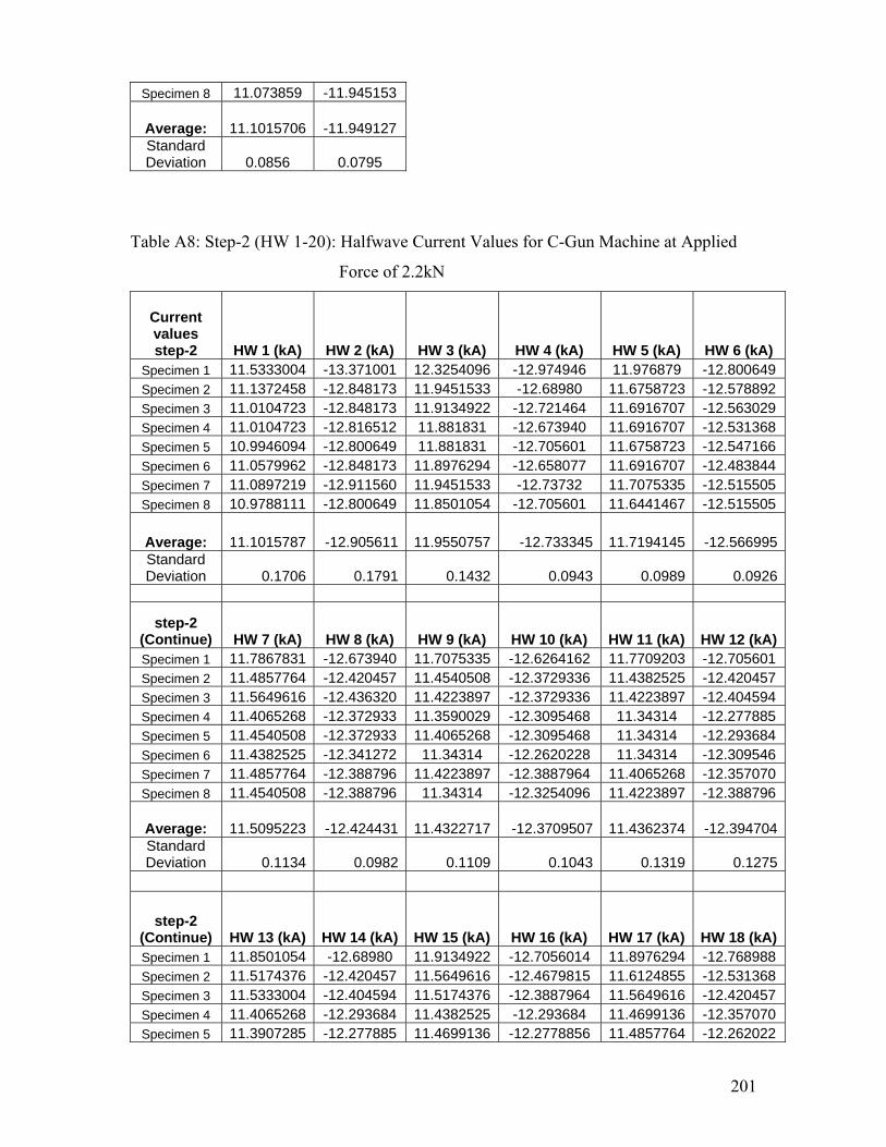
Specimen 8 11.073859 -11.945153

Average: 11.1015706 -11.949127 Standard Deviation 0.0856 0.0795


Force of 2.2kN


Specimen 1 11.5333004 -13.371001 12.3254096 -12.974946 11.976879 -12.800649 Specimen 2 11.1372458 -12.848173 11.9451533 -12.68980 11.6758723 -12.578892 Specimen 3 11.0104723 -12.848173 11.9134922 -12.721464 11.6916707 -12.563029 Specimen 4 11.0104723 -12.816512 11.881831 -12.673940 11.6916707 -12.531368 Specimen 5 10.9946094 -12.800649 11.881831 -12.705601 11.6758723 -12.547166 Specimen 6 11.0579962 -12.848173 11.8976294 -12.658077 11.6916707 -12.483844 Specimen 7 11.0897219 -12.911560 11.9451533 -12.73732 11.7075335 -12.515505 Specimen 8 10.9788111 -12.800649 11.8501054 -12.705601 11.6441467 -12.515505




step-2 (Continue) HW 13 (kA) HW 14 (kA) HW 15 (kA) HW 16 (kA) HW 17 (kA) HW 18 (kA)Specimen 1 11.8501054 -12.68980 11.9134922 -12.7056014 11.8976294 -12.768988 Specimen 2 11.5174376 -12.420457 11.5649616 -12.4679815 11.6124855 -12.531368 Specimen 3 11.5333004 -12.404594 11.5174376 -12.3887964 11.5649616 -12.420457 Specimen 4 11.4065268 -12.293684 11.4382525 -12.293684 11.4699136 -12.357070 Specimen 5 11.3907285 -12.277885 11.4699136 -12.2778856 11.4857764 -12.262022

201

Specimen 6 11.4223897 -12.357070 11.4699136 -12.3254096 11.5015748 -12.404594 Specimen 7 11.4857764 -12.388796 11.5333004 -12.4521187 11.6441467 -12.467981 Specimen 8 11.4540508 -12.404594 11.4540658 -12.3412724 11.5332359 -12.372933


step-2 (Continue) HW 19 (kA) HW 20 (kA)Specimen 1 11.929355 -12.832374 Specimen 2 11.7075335 -12.499642 Specimen 3 11.5808244 -12.420457 Specimen 4 11.4382525 -12.309546 Specimen 5 11.4857764 -12.325409 Specimen 6 11.5649616 -12.357070 Specimen 7 11.7075335 -12.499642 Specimen 8 11.5333004 -12.388796



Force of 2.2kN



202







Average: 12.2758891 -13.075939Standard 0.0574 0.0548

203

Deviation

Table A10: Step-4 (HW 1-20): Halfwave Current Values for C-Gun Machine at

Applied Force of 2.2kN




step-4 (Continue) HW 7 (kA) HW 8 (kA) HW 9 (kA) HW 10 (kA) HW 11 (kA) HW 12 (kA) Specimen 1 12.4679815 -13.418525 12.5788923 -13.4185254 12.6264162 -13.450186 Specimen 2 12.4521187 -13.386864 12.5313683 -13.4501866 12.6264162 -13.481912 Specimen 3 12.4045947 -13.355138 12.4521187 -13.3393403 12.4679815 -13.402662 Specimen 4 12.4679815 -13.450186 12.5155055 -13.4977105 12.5946906 -13.545234 Specimen 5 12.4838443 -13.386864 12.5313683 -13.4501866 12.5946906 -13.481912 Specimen 6 12.5313683 -13.434388 12.6264162 -13.4977105 12.6739402 -13.576960 Specimen 7 12.4045947 -13.402662 12.5788923 -13.4185254 12.5788923 -13.466049 Specimen 8 12.4838443 -13.355155 12.5313038 -13.4343882 12.5947203 -13.545234



204









205







206










207



APPENDIX B

CALCULATED SAMPLE DYNAMIC RESISTANCE PLOTS

208

C-Zange (2.6kN)

0

0.02

0.04

0.06

0.08

0.1

0.12

0.14

HW1 HW3 HW5 HW7 HW9 HW11 HW13 HW15 HW17 HW19

Halfwave

Step 1Step 2Step 3Step 4Step 5Step 6

)(mΩ

Figure B1: C-Gun (2.6 kN) steps 1-6, Dynamic Resistance plot

209

C-Zange (3.0kN)

0

0.02

0.04

0.06

0.08

0.1

0.12

HW1

HW3

HW5

HW7

HW9

HW11

HW13

HW15

HW17

HW19

Halfwave

0.14


Figure B2: C-Gun (3.0 kN) steps 1-6, Dynamic Resistance plot

)(mΩ

210

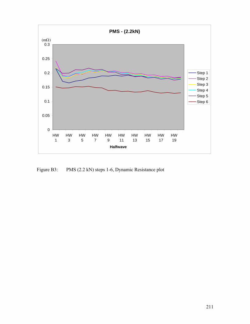
PMS - (2.2kN)

0

0.05

0.1

0.15

0.2

0.25

0.3

HW1

HW3

HW5

HW7

HW9

HW11

HW13

HW15

HW17

HW19

Halfwave


)(mΩ

Figure B3: PMS (2.2 kN) steps 1-6, Dynamic Resistance plot

211

PMS - (2.6kN)

0

0.05

0.1

0.15

0.2

0.25

HW1

HW3

HW5

HW7

HW9

HW11

HW13

HW15

HW17

HW19

Halfwave



)(mΩ

212

PMS - (3.0kN)

0

0.02

0.04

0.06

0.08

0.1

0.12

0.14

0.16

0.18

HW1

HW3

HW5

HW7

HW9

HW11

HW13

HW15

HW17

HW19

Halfwave

0.2



)(mΩ

213

Dalex-25 (1.76kN)

0

0.02

0.04

0.06

0.08

0.1

0.12

0.14

HW1

HW3

HW5

HW7

HW9

HW11

HW13

HW15

HW17

HW19

Halfwave

0.16


Figure B6: Dalex-25 (1.76 kN) steps 1-6, Dynamic Resistance plot

)(mΩ

214

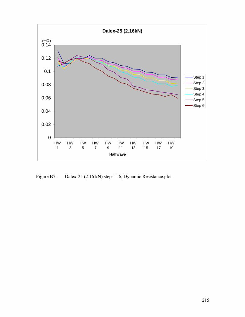
Dalex-25 (2.16kN)

0

0.02

0.04

0.06

0.08

0.1

0.12

0.14

HW1

HW3

HW5

HW7

HW9

HW11

HW13

HW15

HW17

HW19

Halfwave


)(mΩ


215

Dalex-25 (2.2kN)

0

0.02

0.04

0.06

0.08

0.1

0.12

0.14

0.16

HW1

HW3

HW5

HW7

HW9

HW11

HW13

HW15

HW17

HW19

Halfwave


)(mΩ


216

Dalex-25 (2.46kN)

0

0.02

0.04

0.06

0.08

0.1

0.12

0.14

HW1

HW3

HW5

HW7

HW9

HW11

HW13

HW15

HW17

HW19

Halfwave



)(mΩ

217

Dalex-25 (2.6kN)

0

0.02

0.04

0.06

0.08

0.1

0.12

0.14

0.16

HW1

HW3

HW5

HW7

HW9

HW11

HW13

HW15

HW17

HW19

Halfwave



)(mΩ

218

Dalex-25 (3.0kN)

0

0.02

0.04

0.06

0.08

0.1

0.12

0.14

HW1

HW3

HW5

HW7

HW9

HW11

HW13

HW15

HW17

HW19

Halfwave


)(mΩ


219

DZ-35 (2.2kN)

0

0.02

0.04

0.06

0.08

0.1

0.12

0.14

0.16

HW1

HW3

HW5

HW7

HW9

HW11

HW13

HW15

HW17

HW19

Halfwave


)(mΩ

Figure B12: DZ-35 (2.2 kN) steps 1-6, Dynamic Resistance plot

220

DZ-35 (2.6kN)

0

0.02

0.04

0.06

0.08

0.1

0.12

0.14

0.16

HW1

HW3

HW5

HW7

HW9

HW11

HW13

HW15

HW17

HW19

Halfwave


)(mΩ


221

DZ-35 (3.0kN)

0

0.02

0.04

0.06

0.08

0.1

0.12

0.14

HW1

HW3

HW5

HW7

HW9

HW11

HW13

HW15

HW17

HW19

Halfwave


)(mΩ


222

2 4 6 8 10

12

14 16 18 20

0.075

0.085

0.095

0.105

0.115

Halfwave Cycle Time

Ωm

2 4 6 8 10 12 14 16 18 20-0.01

0

0.01

0.02

0.03 Level of Error


Fit Deviation

APPENDIX C

FITTED DYNAMIC RESISTANCE CURVES

Figure C1: Fitted Dynamic Resistance Curve: C-Gun machine at 2.2kN applied

Force.

Data and Fits

223

224

Figure C2: Fitted Dynamic Resistance Curve: PMS machine at 2.2 kN Force.

Figure C3: Fitted Dynamic Resistance Curve: PMS machine at 2.6kN Force.

2 4 6 8 10 12 14 16 18 20

0.19

0.21

0.23 0.25

Halfwave cycle Time

Ωm

2 4 6 8 10 12 14 16 18 20 -0.02

0

0.02

0.04

0.06 Level of Error

Dynamic Resistance

Fitted

Fit Deviation

2 4 6 8 10 12 14 16 18 20 0.195

0.205

0.215 0.22

0.225

Halfwave Cycle Time

Ωm

2 4 6 8 10 12 14 16 18 20

-0.01

0

0.01


Fitted

Fit Deviation

Data and Fits

Data and Fits

Figure C4: Fitted Dynamic Resistance Curve: Dalex-35 machine at 2.2kN Force.

2 4 6 8 10 12 14 16 18 20

0.12

0.13

0.14

Halfwave Cycle Time

Ωm

2 4 6 8 10 12 14 16 18 20 -4

0

4

8 X10-3 Level of error


Fitted

Fit Deviation

Data and Fits

Fit Deviation

4 6 8 10 12 14 16 18 20 0.07

0.08

0.09

0.1

Halfwave Cycle Time

Ωm

2 4 6 8 10 12 14 16 18 20 0

0.005

0.015

0.025 Level of error

Dynamic Resistance

Fitted

Fitted

Figure C5 Fitted Dynamic Resistance Curve: Dalex-25 machine at 3.0kN Force.

225

226

Figure C7: Fitted Dynamic Resistance Curve: Dalex-25 machine at 2.16 kN Force.

Figure C6: Fitted Dynamic Resistance Curve: Dalex-25 machine at 1.76 kN Force.

2 4 6 8 10 12 14 16 18 20 0.08 0.09

0.1 0.11

0.12

Halfwave Cycle Time

Ωm

2 4 6 8 10 12 14 16 18 20 -8 -6 -4 -2 0 2 4 6 8 x 10 -3


Fitted

Fit Deviation

Data and Fits

2 4 6 8 10 12 14 16 18 20 0.09 0.1

0.11 0.12 0.13

Halfwave Cycle Time

Ωm

2 4 6 8 10 12 14 16 18 20 -0.01

0

0.01

0.02


Fitted

Fit Deviation

Data and Fits

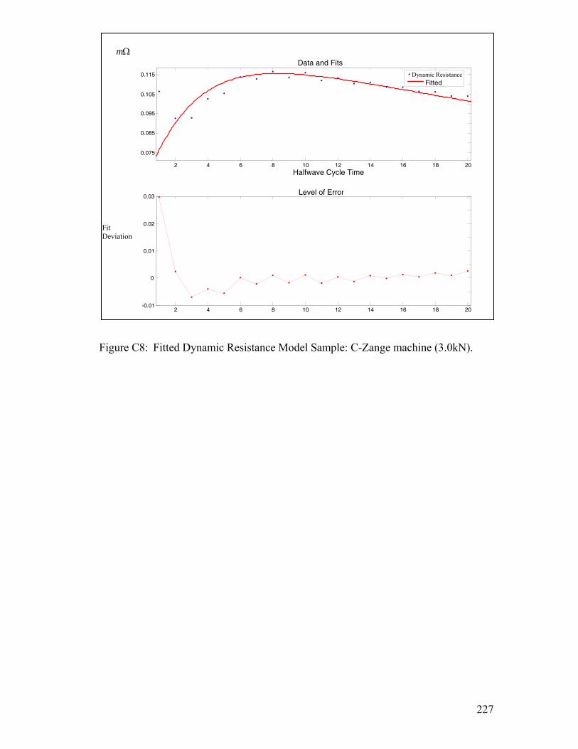
2 4 6 8 10 12 14 16 18 20

0.075

0.085

0.095

0.105

0.115

Halfwave Cycle Time

Ωm Data and Fits

2 4 6 8 10 12 14 16 18 20-0.01

0

0.01

0.02

0.03 Level of Error

Dynamic Resistance

Fitted

Fit Deviation

Figure C8: Fitted Dynamic Resistance Model Sample: C-Zange machine (3.0kN).

227

Figure C9: Fitted Dynamic Resistance Curve: Dalex-25 machine at 2.6kN Force.

2 4 6 8 10 12 14 16 18 20 0.1

0.11

0.12

Halfwave Cycle Time

Ωm

2 4 6 8 10 12 14 16 18 20 -0.01

0

0.01

0.02

0.03 Level of error

Dynamic Resistance

Fitted

Fitted

Fit Deviation

228

APPENDIX D

CODE FOR RUNNING EMBEDDED NEURAL NETWORK MODEL:

PREDICTING SAMPLE RESISTANCE

Private Sub CommandButton1_Click()

Step by step instructions are given on how to use the 'generated DLL for this purpose.

This function returns the network ‘response’.

'Step 1: Create a new neural network object of the NSRecallNetwork type.

'-----------------------------------------------------------------------

'Step 2: Set the pathName of the generated network DLL.

'------------------------------------------------------

The DLL_PATH_NAME below is defined in the Globals module as the 'path to the

newly generated DLL.

nn.dllPathName = DLL_PATH_NAME

'Step 3: Load the saved network weights.

'---------------------------------------

'The initial best weights file is an exact copy of the weights file that was saved

'when the DLL was generated. However, the best weights file will change with each

'run of the TrainNetwork function if the network is reset before training.

nn.loadWeights BEST_WEIGHTS_PATH_NAME

'Step 4: Define the input data.

'------------------------------

'The original breadboard's training input data has been added to this

'workbook in the 'Input' worksheet. This step retrieves the data from this worksheet

229

into an array then 'transposes this array to get it in the right format for input into the

generated DLL.

'The number of inputs in the input data must match the number of inputs

'expected by the generated DLL.

' Dim inputDataTransposed As Variant, inputData As Variant

' inputData = Array(ForceText.Value, DiamterText.Value, KText.Value,

MText.Value, RoText.Value)

Dim inputData(0 To 4, 0 To 0) As Variant

inputData(0, 0) = CSng(ForceText.Value)

inputData(1, 0) = CSng(DiamterText.Value)

inputData(2, 0) = CSng(KText.Value)

inputData(3, 0) = CSng(MText.Value)

inputData(4, 0) = CSng(RoText.Value)

' With ThisWorkbook.Sheets("Input")

' If .Cells(2, 1).CurrentRegion.Columns.Count = 1 Then

' inputDataTransposed = .Range(.Cells(2, 1), .Cells(2, 1).End(xlDown)).Value

' Else

' inputDataTransposed = .Range(.Cells(2, 1), .Cells(2,

1).End(xlToRight).End(xlDown)).Value

' End If

' End With

' inputData = TransposeArray(inputDataTransposed)

'Step 5: Send the input data to the network DLL.

'-----------------------------------------------

nn.inputData = inputData

'Step 6: Get the network response (output).

'------------------------------------------

230

'The network response is assigned to the return value of GetNetworkResponse

'function.

Dim netout As Variant

netout = nn.getResponse

outputText.Value = netout(0, 0)

'Step 7: Release the neural network object.

'------------------------------------------

Set nn = Nothing

End Sub

231

APPENDIX E

CODE FOR RUNNING EMBEDDED NEURAL NETWORK MODEL:

PREDICTING OVERALL PROCESS PARAMETER

Private Sub CommandButton1_Click()

Step by step instructions are given on how to use the 'generated DLL for this purpose.

This function returns the network ‘response’.

'Step 1: Create a new neural network object of the NSRecallNetwork type.

'-----------------------------------------------------------------------

'Step 2: Set the pathName of the generated network DLL.

'------------------------------------------------------

The DLL_PATH_NAME below is defined in the Globals module as the 'path to the

newly generated DLL.

nn.dllPathName = DLL_PATH_NAME

'Step 3: Load the saved network weights.

'---------------------------------------

'The initial best weights file is an exact copy of the weights file that was saved

'when the DLL was generated. However, the best weights file will change with each

'run of the TrainNetwork function if the network is reset before training.

nn.loadWeights BEST_WEIGHTS_PATH_NAME

'Step 4: Define the input data.

'------------------------------

'The original breadboard's training input data has been added to this

'workbook in the 'Input' worksheet. This step retrieves the data from this worksheet

232

into an array then 'transposes this array to get it in the right format for input into the

generated DLL.

'The number of inputs in the input data must match the number of inputs

'expected by the generated DLL.

' Dim inputDataTransposed As Variant, inputData As Variant

' inputData = Array(ForceText.Value, ResistanceText.Value, DiameterText.Value)

Dim inputData(0 To 2, 0 To 0) As Variant

inputData(0, 0) = CSng(ForceText.Value)

inputData(1, 0) = CSng(ResistanceText.Value)

inputData(2, 0) = CSng(DiameterText.Value)

' With ThisWorkbook.Sheets("Input")

' If .Cells(2, 1).CurrentRegion.Columns.Count = 1 Then

' inputDataTransposed = .Range(.Cells(2, 1), .Cells(2, 1).End(xlDown)).Value

' Else

' inputDataTransposed = .Range(.Cells(2, 1), .Cells(2,

1).End(xlToRight).End(xlDown)).Value

' End If

' End With

' inputData = TransposeArray(inputDataTransposed)

'Step 5: Send the input data to the network DLL.

'-----------------------------------------------

nn.inputData = inputData

'Step 6: Get the network response (output).

'------------------------------------------

'The network response is assigned to the return value of GetNetworkResponse

'function.

Dim netout As Variant

233

netout = nn.getResponse

CurrentText.Value = netout(0, 0)

'Step 7: Release the neural network object.

'------------------------------------------

Set nn = Nothing

End Sub

234

APPENDIX F

PREDICTION OF EFFECTIVE CURRENT FOR DESIRED WELD

DIAMETER USING CONTROLLER FORM

N

C-gun Machine with an applied force of 3.0 k

Predicted = 6.703784 Actual = 6.48 Prediction accuracy = 96.55% F1: Effective Current Predicted for C-Gun Machine 3.0kN Applied Force

C-gun Machine with an applied force of 2.6 kN

235

Predicted = 7.98468 Actual = 8.29 Prediction accuracy = 95.29% Figures F2: Effective Current Predicted

for C-Gun Machine 2.6 kN Applied Force

C-gun Machine with applied force of 2.2 kN

Predicted = 7.121756 Actual = 7.1 Prediction accuracy = 99.66% F3: Effective Current Predicted for C-Gun Machine 2.2 kN Applied Force Dalex Machine with an applied force of 1.76 kN

236

Predicted = 5.383359 Actual = 5.18 Prediction accuracy = 96.86% F4: Effective Current Predicted for Dalex Machine 1.76 kN Applied Force Dalex Machine with an applied force of 2.46 kN

Predicted = 6.38831 Actual = 6.58 Prediction accuracy = 97.04% F5: Effective Current Predicted for Dalex Machine 2.46 kN Applied Force Dalex Machine with an applied force of 3.0 kN

237

Predicted = 8.358552 Actual = 8.49 Prediction accuracy = 97.97% F6: Effective Current Predicted for Dalex Machine 3.0 kN Applied Force PMS Machine with an applied force of 2.2 kN

Predicted = 6.474659 Actual = 6.35 Prediction accuracy = 98.08% F7: Effective Current Predicted for PMS Machin

e 2.2 kN Applied Force

PMS Machine with an applied force of 2.6 kN

238

Predicted = 7.986079 Actual = 7.68 Prediction accuracy = 95.28% F8: Effective Current Predicted for PMS Machine 2.6 kN Applied Force PMS Machine with an applied force of 3.0 kN

Predicted = 8.963214 Actual = 9.36 Prediction accuracy = 93.88% F9: Effective Current Predicted for PMS Machine 3.0 kN Applied Force DZ Machine with an applied force of 3.0 kN

239

Predicted = 7.325683 Actual = 7.61 Prediction accuracy = 95.61% F10: Effective Current Predicted for DZ Machine 3.0 kN Applied Force DZ Machine with an applied force of 2.6 kN

Predicted = 8.088946 Actual = 8.32 Prediction accuracy = 96.43% F11: Effective Current Predicted for DZ Machine 2.6 kN Applied Force DZ Machine with an applied force of 2.2 kN

240

Predicted = 6.073895 Actual = 6.49 Prediction accuracy = 93.58% F12: Effective Current Predicted for DZ Machine 2.2 kN Applied Force

241

APPENDIX G

PAPER SUBMISSION 1

MODELLING DYNAMIC RESISTANCE VARIABLE IN RESISTANCE SPOT WELDING

Pius Nwachukwu Oba, Professor D. Chandler and Dr. S. Oerder

(University of the Witwatersrand, Johannesburg, South Africa)

Prof. Dr.-Ing. Dr. h.c.L. Dorn and Dr. Ing. Kevin Momeni

(Technical University Berlin, Germany)

Abstract

The non linear and complex nature of dynamic resistance variables makes it difficult to

predict weld quality. Presented in this paper is the method used to obtain appropriate

models for predicting weld resistance from dynamic resistance halfwaves.

An empirical three parameter approximate mathematical function model with dependent

and independent variables was developed for curve fitting the nonlinear halfwave

dynamic resistance curve. The values of the parameters were used for determining overall

resistance for any desired weld diameter. The prediction capability of the empirical model

for predicting resistance in any welding machine was improved by passing the outputs

from the empirical model through neural network learning. By using the multilayer

perceptron (MLP) neural network architecture, resistance of each sample was predicted

with an accuracy of about 99.9% to 97%. This estimated resistance can be used for

predicting weld quality with good reproducibility.

242

APPENDIX H

PAPER SUBMISSION 2

MODELLING RESISTANCE SPOT WELDING PARAMETERS FOR PREDICTING EFFECTIVE WELD CURRENT





Abstract

Presented in this paper is a model used for predicting effective weld current (RMS) for

desired weld diameter (weld quality) in the resistance spot welding process. Electrical

parameters namely effective weld current and dynamic resistance with applied electrode

force, are identified as the strongest input signals necessary to predict the output weld

diameter. These input parameters are used for developing a neural network process model

for predicting effective weld current.

An initial empirical model developed by the authors as was used for predicting sample

resistance which was integrated with this model for predicting required effective weld

current for any desired weld diameter. The prediction accuracy of this model was in the

range of 94% to 99%. This neural network process model was designed by optimising

the squared error between the neural network output and the desired output. The neural

network process model delivers effective current for any desired weld diameter. The

model is observed to predict the desired output accurately.

243

APPENDIX I

PAPER 3 DEVELOPED FOR PUBLICATION

CASE STUDY ON IMPROVING NEURAL NETWORK PREDICTIVE CAPABILITY

APPLICATION IN RESISTANCE SPOT WELDING QUALITY MODELLING





Abstract

A three parameter approximate mathematical function model with dependent and

independent variables was used for curve fitting nonlinear halfwave dynamic resistance

curve generated from the resistance spot welding process. The value estimates of the

parameters were used to develop charts for determining overall resistance of samples for

any desired weld diameter. The prediction error in estimating sample resistance using the

charts was 16% to 167%.

The empirical model prediction accuracy was improved using neural network artificial

intelligency to learn the pattern in the dataset. The two inputs used were applied electrode

force and weld diameter while calculated sample resistance from the empirical model was

the output. These dataset were used to train four neural network types. These were the

Generalised feed forward neural network, Multilayer perceptron network, Redial basis

function and Recurrent network. Of all the four network types, the multilayer perceptron

had the least mean square error for training and cross validation with prediction error of

65%. Prediction improvement from previous 167%.

244

245

The number of input parameters in the multilayer perceptron architecture was increased

from the initial two inputs to five inputs by including all the estimation parameters from

the mathematical model. This Multilayer perceptron neural network architecture yielded a


correlation coefficient in testing of 0.999 and maximum estimation error of about 0.1% to

3%. An accuracy of 99.9% to 97%.

246

UAPPENDIX J

UPAPER 4 DEVELOPED FOR PUBLICATION

DESIGN AND IMPLEMENTATION OF PREDICTIVE CONTROLLER FOR THE

RESISTANCE SPOT WELDING PROCESS.





Abstract Presented in this paper is the method used for the design of a predictive controller for

predicting effective weld current in the resistance spot welding process using a developed

process model. A suitable process model forms an important step in the development and

design of process controller for achieving good weld quality with good reproducibility.

The process model developed by the Authors consists of three parameter empirical model

with dependent and independent variables used for curve fitting the nonlinear halfwave

dynamic resistance curve. To improve the prediction accuracy of this empirical model,

the data generated from the model were used to train four different neural network types.

Of the four network types trained, the MLP had the least mean square error for training

and cross validation of 0.00037 and 0.000390 respectively with linear correlation

coefficient in testing of 0.999 and maximum estimation error range from 0.1% to 3%.

This model was selected for the design and implementation of the controller for

predicting overall sample resistance. Using this predicted overall sample resistance, and

applied electrode force, a similar model was developed for predicting required effective

weld current for any desired weld diameter. The prediction accuracy of this model was in

247

the range of about 94% to 99%. The controller outputs effective current for any desired

weld diameter. This controller is observed to track the desired output accurately with

same prediction accuracy of the model used which was about 94% to 99%. The controller

works by utilizing the neural network output embedded in Microsoft Excel as a digital

link library.

quality analysis and predictive control modelling of …

Documents