Product Market Characteristics and the Industry Life Cycle

Kenneth L. Simons *

May 1, 2011

*Economics Department, Rensselaer, 110 8th Street, Troy, NY 12180, USA. Phone 1 518 276 3296, fax 1 518 276 2235, email simonk@rpi.edu, web www.rpi.edu/~simonk. Acknowledgments: Steven Klepper kindly gave permission to use US data which the author helped to collect. Teams of research assistants worked to assemble and verify data at Carnegie Mellon University and at Royal Holloway, University of London. Chris Mega, Avi Bar, and Alessio Puricelli provided especially substantial research assistance. Chunbo Ma at Rensselaer also helped clean the US data. The inter-library loan office at Carnegie Mellon and the Guildhall Library in London went to special efforts to provide parts of the hundreds of shelf-feet of trade directories used. Graham Hogg advised regarding UK ball point pen makers. Valuable comments came from participants, commentators, and anonymous reviewers of conferences of the Academy of Management, American Economic Association, Centre for Economic Policy Research, European Association for Research in Industrial Economics, Industrial Organization Society, International Schumpeter Society, Network of Industrial Economists, International Workshop on the Post-Entry Performance of Firms, and at seminars at Chalmers University of Technology, Ente Einaudi (Bank of Italy), the LSE, Cornell University, Rensselaer, and the Universities of Connecticut, Oklahoma, Sussex, Toronto, and Waterloo.

Product Market Characteristics and the Industry Life Cycle

Abstract

A theoretical model implies that technological opportunity drives industry evolution, fueling a spiral of advantage that allows a few firms to dominate in the long run in high technological opportunity markets. Distinctive implications are tested using new long-period, cross-sectional, cross-national (US and UK) industry data on narrowly-defined product markets.

The process by which industries evolve to their static outcomes is found to occur similarly for the same industry in the different countries. Some industries have strong shakeouts in firm numbers and others not, confirming findings of Gort and Klepper (1982) on the first large set of alternative data. In industries with shakeouts entry eventually nearly ceases, but in industries without shakeouts entry remains high. Even in strong shakeouts there is not necessarily a rise in firms’ rate of exit coincident with the shakeout, confirming that shakeouts are not driven by single technological events. The theory and evidence explain why early mover advantage is tied up with the spiral of firm advantage that yields shakeouts, so that only in industries with substantial shakeouts do early movers experience low exit rates relative to incumbents.

Technological patterns conform to those expected if technological opportunity drives typical industry outcomes. Leading early entrants dominate relevant patents in industries with substantial shakeouts, and patenting enhances survival especially in industries with shakeouts. Thus technological innovation seems typically to drive alternative industry competitive dynamics, through a spiral of firm advantage in industries with high opportunity for product improvement and process innovation. Keywords: Industry Dynamics, Cross-National Comparison, Technology, Product Life Cycles

1

1. Introduction

Industries with high or low concentration in one nation tend to have similar high or low

concentration in all industrialized nations (Bain, 1966; Pryor, 1972). This finding suggests, in

the words of Schmalensee (1989, p. 992), that “similar processes operate to determine

concentration levels everywhere….” Since national markets are somewhat independent,

moreover, it seems that concentration is substantially predictable based on traits of the

technology or product.

This study extends cross-industry, cross-national empirical research by examining not the

static outcomes studied in the 1960s and 1970s, but the historical process through which

industries move toward long-run outcomes. A theory of industry evolution is used to suggest

what type of industries will experience shakeouts, the reasons for shakeouts, and cross-national

relationships in the degree and timing of shakeouts and in shifting patterns of entry. New cross-

national, cross-industry data for competitive-level industries, collected longitudinally from at or

near the inception of each industry, are used to probe how industry outcomes are formed. The

evidence facilitates distinctive tests of the causal process by which a characteristic such as

internal-to-the-firm technological opportunity may drive early-mover advantage and shakeouts.

The empirical strategy is that, if economic models are correct about how internal-to-the-

firm technological opportunity typically drives early-mover advantage and industry shakeouts,

three predictions should hold. First, comparing the same industry across two or more countries,

a similar competitive outcome should occur in all nations in which the industry initially

developed. Thus systematic causes, not differing national environments (Lundvall, 1992;

Nelson, 1993) nor random successes and failures of firms, would seem to drive industry

outcomes. Second, correlated patterns of entry, exit, early-mover advantage, and shakeout

2

should be observed, potentially allowing types of competition can be classified into a few (here,

two) commonly-occurring groups. Differences in exit timing facilitate tests between alternative

theories of industry shakeouts. Third, measures of technology should be correlated with the

entry, exit, early-mover, and shakeout patterns, so that technological activity and its effects are

strongest in industries with early-mover advantage and shakeouts. This would provide evidence

that within-firm technological opportunity could be the primary trait underlying differences in

industry evolution.

The three predictions are confirmed using data on manufacturing industries in the United

States and the United Kingdom. In years with limited international trade, both the timing of an

industry’s shakeout and its resultant percentage drop in number of firms are highly and

significantly correlated. In industries with substantial shakeouts, but not in industries with little

or no shakeouts, entry eventually nearly ceases and an early-mover advantage is apparent in exit

rates. Estimates imply that in industries with very severe shakeouts the annual percentage exit

rate is lower by 3.4 for the first half of entrants compared to the second half, whereas in

industries with no shakeout the annual percentage exit rate is higher by 2.2 for the first half of

entrants. Exit rates typically remain comparable throughout an industry’s history; the shakeouts

are “shake-ins” in which entrants populate an industry in early decades while exit steadily

whittles away the population of firms. In industries with substantial shakeouts, early entrants

typically dominate at generating relevant patents. Having patented in the previous five years is

associated with a 2.4 lower percentage annual exit rate in industries with no shakeout, but with a

6.7 lower percentage annual exit rate in industries with near-total shakeouts.

Identification is complicated by international trade which could drive cross-national

similarities, and by endogeneity between the dependent variable exit and the degree of shakeout

3

which is involved as an interaction in key regressors. The analyses therefore consider

restrictions of cross-national comparisons to years preceding international trade, and exit models

that use the other nation’s percentage drop in number of firms, in all years or years preceding

strong international trade, as a tool for instrumentation. The findings are robust to these

identification strategies.

This study provides evidence that internal-to-the-firm technological opportunity may be

these industry dynamics’ driving characteristic. However, could another (correlated)

characteristic such as opportunity for advertising (Sutton, 1991), or distribution networks, in fact

drive the observed patterns? In two industries studied here, tires and television receiver

manufacturing, Klepper and Simons (2000a, 2000b) find evidence that technological innovation

drove shakeouts while advertising or distribution networks had an independent effect (in tires) or

no effect (in televisions) on firm exit. Direct evidence on how technological innovation in firms

unceasingly drove four industry shakeouts is in Klepper and Simons (1997). Nonetheless, more

work is needed to confirm how often opportunities for technological innovation versus

advertising, distribution, or other traits might in practice yield industry shakeouts.

A model of industry shakeouts developed in section 2 yields the three predictions stated

above. Data are described in section 3, and empirical tests are reported in section 4. Section 5

discusses the results and concludes.

2. Technological Change and Market Structure Dynamics

To posit a logic behind how an industry characteristic, in-house research and engineering

(R&E) potential, can drive different product industries to experience shakeouts or not, to become

concentrated among a few producers or not (necessarily), and to drive a growth of relative

advantage that drives such concentration, this section presents a theory of industry dynamics.

4

The theory builds in a simple, yet extremely important, manner on models of industry shakeouts

developed by Klepper (1996, 2002). The most minimal cross-national difference, country size,

and a simple parameter for cross-industry difference, R&E potential, are added to the models.

Klepper’s theories characterize how entrants gradually populate and expand output in a

new industry. Businesses differ in the capability of employees and in their entry times, with the

more capable and larger businesses experiencing the greatest returns to research spending, and

therefore choosing to invest the most in research. Their investments yield greater financial

returns to output and hence incentivize the greatest rate of expansion. As a result, the state

variable firm size cumulates most for these leading firms, giving them, at least in a relative

sense, a rich-get-richer advantage that ensures there continuing dominance over other firms. The

profits of firms and entrants vary, with some firms steadily pushed out of the market as rising

industry output drives down the representative price and makes marginal firms’ profits negative,

and with entry eventually ceasing when the prospective profits of all potential entrants become

negative making entry unattractive. The cessation of entry coupled with ongoing exit causes a

drop-off or “shakeout” in firm numbers following the initial build-up of firms.1

A. Model

Assume that a new product technology is introduced in independent nations n = 1,2,…

which are identical except in their population base bn which is normalized to 1 in nation 1.

Buyers in each nation face a reference price pnt determined by the inverse demand function

pnt = f (Qnt / bn; Rt ) , where f (⋅) decreases with industry output Qnt put on a per-person basis by

1 As in Klepper (2002), product and process research are treated identically, both to provide a simpler starting point,

and to reflect available fact about the roles of product and process innovation (Klepper and Simons, 1997).

5

dividing by bn , and increases with worldwide cumulative knowledge Rt which enhances all

firms’ products. The potential for knowledge improvement is measured by parameter α ≥ 0 .

Each nation has bn Kt potential entrants in period t. Potential entrants i differ in ability

ai > 0 , with upper limit a and continuous distribution H (a) . Each entrant firm has output Qit

which starts at 0 before entry and increases each period by Δqit = Qit −Qit−1 . This growth has

cost m(Δqit ) , which is convex with a minimum of 0 at Δqit = 0 , reflecting high costs of rapid

expansion such as discussed by Penrose (1959) and modeled in convex form in Flaherty (1980)

and in a large literature on optimal control and growth.

In addition to choosing Δqit , the firm chooses R&E spending rit , which affects period t

profit only; after t technology becomes common knowledge and instead enhances overall

demand through the term Rt . Price minus average production cost is pnt − c(Rt ) + l(αairit ) ,

whose terms are price, an initial unit cost c(Rt ) > 0 with ′c (⋅) < 0 , and the term l(αairit ) which

represents the benefits of research. Research reduces cost and/or improves the firm’s product

such that it can charge a price above the reference price in period t. Research is always

beneficial at the margin, ′l (⋅) > 0 , but it has diminishing returns ′′l (⋅) < 0 since firms first cherry

pick the best projects available to them in period t. The argument to l(⋅) equals R&E spending

multiplied by α and by ai , so that the research inputs are scaled by industry-wide R&E potential

and by firm-specific R&E ability.

Profit is therefore Πit = ( pnt − c(Rt ) + l(αairit ))Qit − rit − m(Δqit ) . Firm i’s only state

variable is Qit . To simply convey the model’s points, we follow Klepper by assuming myopic

decision making that maximizes current-period profit. Potential entrants enter if their first-

6

period profit would be positive, and exit if their profit would be negative. (Infinite-horizon

decision making, it can be shown, yields similar outcomes). Firms have a random failure

probability χ at the end of each period due to external causes.2 The first-order conditions are, if

α > 0 ,

′m (Δqit* ) = pnt − c(Rt ) + l(αairit

* ) ,

′l (αairit

* ) = 1αai (Qit−1 + Δqit

* ).

A further assumption about the form of the research production function, ′l (0) > 1

αaiQmin

where

Qmin is the smallest firm size observed in practice, guarantees an interior solution (Klepper,

2002).3 If α = 0 , rit* = 0 and ′m (Δqit

* ) = pnt − c(Rt ) . With α > 0 , most of the conclusions of

Klepper (1996, 2002) follow with little modification of the proofs. It is assumed that in each

period Rt is small enough that pt < ( pt−1 − δ) for some δ > 0 ; this abstracts away from the

possibility of product popularity gains that outpace industry expansion. With α = 0 , ability is

irrelevant, there is no R&E, and entry and firm expansion continue until Qnt reaches a steady

state where Πit = 0 and entry and growth are just sufficient to replace random exit.

2 This failure condition is a simplified version of Klepper’s (2002) productivity shock, and can be made a decreasing

function of pni − c(Rt )+ l(αairit* ) without change to the conclusions. It can alternatively be made a decreasing

function of Πit but this adds the complication that industries without R&E could have some shakeout depending on

the steepness of the function and other conditions. 3 More properly, the Inada condition

limρ→0+

′l (ρ) = ∞ can be imposed on the research production function.

7

B. Testable Implications

The theory has distinctive implications for cross-national and cross-industry differences

in the dynamics of competition. These implications hold for industries defined at a competitive

level: products produced by different firms should be substitutable enough that they could fulfill

the same consumer need, so that firms compete directly with each other in terms of price and

quality. Product differentiation may exist but most not be complete.

Comparisons across countries apply to capitalist economies in which an indigenous

industry producing the product develops near the worldwide commercial inception of the

product.4 The theory, in its characterization that the only cross-national differences are captured

by bn , yields identical outcomes in each nation except that the number of firms is proportionate

to bn . It provides a logic why international trade should be limited, since firms would derive no

benefit by selling to markets in other nations instead of in their home nations, partially justifying

the theory’s assumption of independence across nations. To the extent that in practice different

nations’ industries indeed are isolated, the ideal that industry outcomes should be the same

across nations can thus be carried out. While this ideal depends on strong assumptions about

comparable numbers of entrants, firm ability distributions, and demand functions, it sets a

benchmark for comparison to outcomes that might be driven by random causes or national

environments, yielding different patterns of entry, initial modes of competition, times with peak

numbers of producers, or fractions of weaker firms that might exit during later competition.

Hypotheses 1 and 2 pertain to the number of firms as it changes over time. The theory

taken literally predicts identical graphs of the number of firms versus time, simply scaled in

4 Comparisons might also hold for planned economies, if economic realities force the planners to make decisions

approximating those of capitalist firms and if in practice much R&E must occur within individual productive units

and diffusion across units occurs about as slowly as in capitalist economies.

8

proportion to bn , and hence indicates that the time with the peak number of firms and the degree

of shakeout, defined as the percentage drop in number of firms from its peak, should be identical.

In particular, higher R&E potential is associated with an earlier and more rapid shakeout of

firms. Hence, substituting the term “similar” in place of “identical” to allow for limited

differences in functional forms, the spirit of the theoretical prediction is captured as:

HYPOTHESIS 1: The same product industries in different countries experience similar degrees

of shakeout.

HYPOTHESIS 2: The same product industries in different countries experience similar timing as

to when they achieve their peak number of firms.

Hypotheses 3 and 4 pertain to the entry and exit processes causing changes in the

numbers of firms. Less entry per year or greater percentage exit per year each could cause a

drop in the number of firms. In this theory, however, the decrease in entry guarantees a

shakeout, while the annual percentage of firms exiting the industry may remain steady. In

industries with no R&E potential ( α = 0 ), however, entry continues and no shakeout occurs. A

advantage of earlier entrants is another telltale sign that should be associated with shakeouts;

although exit continues in industries with and without shakeouts, the exit rate of relatively early

entrants is low relative to later entrants in industries with shakeouts (where α > 0 ), but not in

industries without shakeouts (where α = 0 ).

This contrasts with other theories of shakeouts, in which a single new technology or the

standardization of product designs triggers a shakeout. In those cases, the probability of exit

should rise at the start of the shakeout, but should subsequently decline (Utterback and Suárez,

1993; Jovanovic and MacDonald, 1994). Likewise, in these views the extent of early-entrant

9

advantages is commonly anticipated to grow at the time of the shakeout and then diminish. If

these views are right, while entry would be expected to decline as in this theory, the difference is

that exit must increase at the time of the technological event triggering the shakeout and then

decline as surviving firms have adapted to the technological change.

The following Hypotheses 3 and 4 therefore should be expected to hold in the long term

if continuous R&E matters for competition.

HYPOTHESIS 3: In industries with strong shakeouts, entry eventually declines considerably, but

the rate of exit need not increase. In industries with little or no shakeout, entry continues

relatively unabated, and exit continues. Countries that simultaneously developed a substantial

population of producers in an industry experience similar declines (or lack thereof) in entry.

HYPOTHESIS 4: In industries with strong shakeouts, firms in earlier-entering cohorts tend to

exit less frequently than firms in later-entering cohorts. With little or no shakeout, these

differences are insignificant or nonexistent.

Hypotheses 5 through 7 pertain to the potential for R&E and inter-cohort differences in

firm R&E activities. A greater potential for R&E causes shakeouts in the model because it

yields substantial R&E output (hypothesis 5) that is dominated by the largest producers, which

predominantly entered earlier (hypothesis 6) and achieve reduced probability of exit as a result of

their R&E successes (hypothesis 7):5

5 The theoretical view also implies that with little or no shakeout, entrants from all eras are similar in their near-zero

R&E output. Unfortunately, the sample sizes involved should then make it virtually impossible to test statistically

for similarity in amounts of R&E output. Two other complicating factors arise in testing hypotheses 5 and 6. First

is the potential for product development that does not qualify as R&E, or for R&E that can be successfully sold

between firms. If the incentives for product development and saleable R&E are similar in shakeout and non-

shakeout industries, R&E data that are polluted with development and saleable R&E will tend to suggest similar

10

HYPOTHESIS 5: In industries with strong shakeouts, improvements in the product and

manufacturing methods tend to be more rapid than in industries without shakeouts.6

HYPOTHESIS 6: In industries with strong shakeouts, relatively early entrants have the greatest

R&E output.

HYPOTHESIS 7: In industries with strong shakeouts, firms with relatively high R&E output have

relatively low probability of exit from the industry. This is less true in industries with little or no

shakeout.

C. Discussion of the Theory

Why might earlier entrants hold a technology-related advantage? Two reasons

emphasized in the economic literature are cost-spreading, as firms that have entered earlier and

had time to grow larger can do R&E to improve quality or unit cost and spread the cost over a

greater number of units produced, and progressive cost reduction (and progressive quality

improvement, both responsible for learning curves).7 Although the theory presented here is

based on cost spreading, it would be possible to develop a variant of progressive cost reduction

output for earlier and later entrants. Second is inter-industry differences in propensity to patent or record an

innovation, or in how dramatic an innovation needs to be before it is patented or recorded as an innovation, which

add substantial noise to inter-industry comparisons regarding prediction 5. 6 The expression “tend to be” is necessary because in some cases rapid improvements can be purchased through

third-party suppliers, as for styrene manufacturers buying process machinery from third-party suppliers, or diffusion

of technological information may be easy and rapid. 7 On cost-spreading, see for example Flaherty (1980) and Shaked and Sutton (1987). On progressive cost reduction

and learning curves, Petrakis, Rasmusen, and Roy (1997) address the issue of industry shakeouts.

11

theories with similar implications.8 Non-technological forces such as advertising cost spreading

could yield similar outcomes.

The focus here is on research and engineering, not development of new kinds of products,

hence the use of the term R&E which is a subset of R&D. Development of new products that are

not close substitutes for the original creates new markets, with their own competitive dynamics,

largely or entirely independent of competition in the original market.9 Development of product

features that enhance the existing product or create variants of it is included in R&E.

In addition to focusing on R&E excluding development of non-substitutable products, the

focus is on research that is difficult to license and sell to other firms. Technologies that can be

effectively sold provide relatively similar incentives to small and large firms to develop

innovations, because the innovations can be sold for similar amounts of profit regardless of the

size of the innovator; this would undermine the tendency of large (and hence mainly early-

entering) producers to dominate innovation. Hence it is the potential for within-firm R&E, not

for development or for readily saleable innovation, that is expected to matter to inter-industry

differences in competitive dynamics.10

8 Cost-spreading, with a continual need for new R&E work, is assumed in the model used to develop hypotheses

here. In contrast, progressive cost reduction theories typically assume a fixed stock of achievable R&E, resulting in

an eventual lessening of competition as R&E opportunities become exhausted. 9 If firms create new variants of the existing product, satisfying the same consumer need as the original product, the

variants are characterized here as quality changes. 10 Both product and process R&E are expected to matter for firm technological competitiveness, and they are

expected to continue being competitively relevant throughout the parts of the industry life cycle analyzed

empirically here. A shift in importance from product to process R&D over the industry life cycle is depicted as

common by Abernathy and Utterback (1978; Utterback & Abernathy, 1975). However, such a product-process shift

has not generally been borne out in empirical studies, which might better be characterized as showing the continuing

importance of both types of innovation (McGahan & Silverman, 2001). It is implicitly assumed here that where

technological opportunity for R&E is strong initially, that opportunity is rarely if ever exhausted quickly. This

assumption appears to fit well with studies of technological innovation in industries (cf. Mansfield, 1968).

12

3. Data

Assessment of the theoretical view, and of the more general questions of similarity and

predictability in industry outcomes, requires data over many decades, beginning at or near the

inception of a product market. Data for each product must be at the competitive market level;

producers included must make products that are close substitutes for each other. Moreover, a

test of the first prediction requires data for the same products in more than one national market.

Neither data collected by national statistical agencies nor cross-industry data from commercial

services fully meet these needs.11 Instead, this study bases its sample on the studies of industry

dynamics by Gort and Klepper (1982) and Klepper and Graddy (1990). Those authors examined

46 U.S. manufactured products from the early 1900s up to 1970 and 1980 respectively, using

counts of numbers of manufacturers drawn from annual editions of Thomas’ Register of

American Manufacturers. To carry out the tests proposed, much more detailed data than the

numbers of firms recorded in the original study were collected in both the U.S. and the U.K.

Data for additional countries would be helpful, but for this study (the first many-industry

international study of its kind), the focus was restricted to these two countries given the

enormous difficulties and expense involved in data collection. In the U.K., the annual Kelly’s

Directory of Merchants, Manufacturers, and Shippers was identified as a source. Among the 46

products first studied by Gort and Klepper (1982), products were used if Kelly’s Directory

11 Data from government censuses of firms and many commercial datasets are available generally at 4-digit or more

aggregated SIC levels. At these levels, most of the products made by companies are not substitutable; a customer

would rarely buy a hearse, bus, or armored personnel carrier as a substitute for an automobile (all are in 1987 U.S.

SIC 3711). Government and some commercial data sources also tend to recognize new industries only after

substantial delay, making it impossible to analyze the important early years of competition. Also, census and other

data sources classify firms into the industries in which they have the greatest productive activity, but many firms

produce in multiple 4-digit industries and hence are ignored in such data in all but their primary industry.

13

included similar categories. This process yielded 18 products with closely matched definitions

for product categories.

A. Firms

Annual editions of Thomas’ Register and Kelly’s Directory were consulted to determine

the identities of firms that manufactured each product in each year for which data were available,

up to a maximum year described below.12 Firm entry and exit dates were determined using these

annual data. Addresses were also recorded and, in the absence of further information, an

identical address in the same or nearby years was taken as evidence that differently-named firms

were parts of the same organization. A firm is defined, as in relevant theories, not as a legal

entity nor by its owners, but by the facilities, equipment, and skilled personnel it possesses.

In selected industries, additional sources were used to check the identities of firms and

their histories of production, merger, and acquisition, and this information was integrated with

the data. Perhaps because most of the firms in the sample are small, mergers or acquisitions

involving multiple firms in a product market account for only a tiny percentage of exits recorded

in the data, and hence the lack of systematic information on mergers does not appear to bias the

results. Moreover, when acquisitions occurred, they appear almost always to have involved

firms close to failure, so that treating acquisition as exit may indeed be the most appropriate

treatment for testing the hypotheses. In the U.S., an additional directory, Television Factbook,

was identified as a more reliable source for data on two products, televisions and television

picture tubes, and this source is used instead of Thomas’ Register.13

12 In Kelly’s Directory, although the product categories had headings indicating the firms listed were manufacturers,

additional firms were occasionally included with an annotation that they supplied components or sold rather than

manufactured the product; these non-manufacturers of the products are excluded from the data. 13 Klepper and Simons (2000b) discuss Television Factbook as an information source.

14

The data in Thomas’ Register and Kelly’s Directory are neither perfectly accurate nor

based on perfectly commensurate product definitions, but the two trade registers do seem to yield

fairly accurate and comparable listings for many product categories.14 Products were therefore

classed in two groups, labeled as having somewhat reliable versus more questionable data

sources. Products classed as more questionable are those with few manufacturers in one of the

countries and those with quite ambiguous product definitions. Analyses are based primarily on

products classed as somewhat reliable, although counts of the numbers of firms in each year are

compared for the more questionable product categories as well.

Data were collected through the 1980 editions of the registers, published in 1979, to

provide at minimum several decades in which to analyze each product. In one product,

television picture tubes, the US data end at 1971 because the source used ceased listing the

category. For two products with extremely severe shakeouts, tires and televisions, extended data

were collected to allow further study: the data collection period was limited to 1980 in US tires

due to a change in category definitions, but other data were extended to 1996 for UK tires, 1989

for US televisions (the data source ceased listing television manufacturers after 1989), and 1996

for UK televisions. Statistical comparisons between nations are restricted to end at the last year

when data are available for both nations.

14 As an example of incommensurate product definition, the tires listings for the US were limited to pneumatic (and

a few cushion) automobile tires whereas the UK lists included some solid and non-automotive tires. It is usually

possible to judge the degree of product definition differences and ambiguities given the names of categories in the

registers, annotations next to firms’ names about the kinds of products they supplied, or the firm names themselves.

Ambiguities in types of firms could arise because the registers sometimes included sellers, repair shops, importers,

or related service providers among the lists. Such non-manufacturers generally are few among the lists (the

registers’ publishers made concerted efforts to limit the relevant lists to manufacturers), and annotations and firm

names again provided clues to gauge the (apparently very limited) extent to which they polluted the data.

15

B. International Trade and Multinational Producers

As a measure of years with strong international trade, years once US imports attained

10% of shipments were identified. Where early data were not available, low imports in years

with available data were assumed to signal limited international trade to date. Imports data stem

from the NBER international trade database (Feenstra, 1996) and value of domestic shipments

data stem from the NBER Productivity Database (Bartelsman and Gray, 1996). Data pertain to

the 4-digit 1972 SIC category containing a product. Lasers and artificial Christmas trees are

excluded in analyses that exclude years with strong international trade, due to difficulty

determining an appropriate and reasonably narrow category. For typewriters, substantial

international trade was occurring by the first year of the NBER data, and US government sources

cited in Frederiksen (1974, p. 250-251) were used. Radar was included based on evidence of

limited international trade in U.S. Department of Commerce (1991).

Foreign-originated producers were identified where possible using literature about each

product.15 A firm is treated as foreign-originated if it made the product in another country before

beginning in-country production. Generally a relatively small number of foreign producers enter

the industry and tend to do so in later years. Because of their earlier entry date in their original

country, and their large size and high skill (given their international success), foreign-originated

producers typically have long lifetimes after entry relative to most in-country producers, as well

as high R&E output. Given their small numbers, foreign producers have a limited effect in

counts, but because they tend to have large research programs and enter late they would have a

particularly strong effect on analyses of exit and R&E. Foreign-originated firms therefore are

removed from the sample in analyses of entry, exit, and patenting.

16

C. Research and Engineering

Patent data provide a systematic source of information to analyze technological change

across all of the products (other measures of R&E could not systematically be obtained). US and

UK patent data from 1920 onward were obtained from the EPO Worldwide Patent Statistical

Database. Relevant patent categories and/or title keywords were determined for each of the

products examined here, and all relevant patents in the database were catalogued along with all

available information about the assignee and the date each patent was granted. The resulting

patents were matched to firms in the sample, and a random sample of the patents of each firm in

each product was selected and the patent titles, and if necessary abstracts and full patents, were

consulted to ascertain whether the invention seemingly applied to the improvement of the

existing product or its production methods. If a substantial fraction of inappropriate patents was

found, inappropriate types of patents were excluded by ruling out all patents whose titles

included certain combinations of words that signal bad fit; this procedure was repeated until the

sample was cleansed of at least most non-R&E-related patents.

4. Empirical Tests

A. Trends in the Number of Firms: Cross-National Comparison

Hypotheses 1 and 2 are tested by comparing how the number of firms changed over time

in matched product markets in the US and the UK. The counts of firms can be used to assess

whether identical product markets did or did not experience shakeouts in both nations, as well as

the timing and severity of shakeouts. Table 1 compares for the two nations the year with the

peak number of firms in each product, and the percentage decrease between the peak and the

15 Sources include Martin (1925), Carlip (1960), King (1966), Arnold (1985), Willer (1994), Adler (1997), and

Gostony and Schneider (1998).

17

lowest subsequent number of firms. If multiple years share the peak number of firms, the latest

such year is reported. The table is divided into two panels according to the apparent reliability of

data sources. All of the product categories collected from the registers involved some

ambiguities in product definition and in the types of firms included, and some products involved

small numbers of firms and therefore substantial random variation in measures such as the peak

year, but the ambiguities and random variation appear to be relatively small in the first panel

versus substantial in the second panel.

Within each panel, products with the largest percentage drop in US firms are listed first.

Despite presumed errors in the data, the patterns tend to be remarkably similar across the two

nations. In panel A, the first five products exhibit percentage decreases in number of firms that

are always within 10% of each other. The remaining four products exhibit more substantial

differences in the percentage drop in number of firms, but even so there is still a tight correlation

between countries even with these more disparate figures. The close cross-country relationship

in each industry’s degree of shakeout is remarkable.

Even more remarkably, the year with the peak number of firms is also substantially

related within each product across the two nations. A majority of the products had differences of

less than one decade in the timing of the peak number of firms. This suggests that not only do

product market characteristics determine the degree of shakeout in an industry, but moreover

product characteristics may to a substantial degree determine the timing of when shakeouts

begin. One interpretation of this pattern, consistent with empirical studies of shakeouts, is that

the rate at which competition intensifies is a function of technology development and usage that

tends to be fairly predictable and not easily influenced by national economic environments or

random outcomes.

18

In panel B of the table, problems with the data sources make it difficult to observe the

true relationship between the two countries’ patterns. Despite the considerable noise in the data,

however, the percentage drop and especially the peak year show substantial positive

relationships across countries. Again, to the extent a pattern can be seen through noise in the

data, product-specific characteristics seem to be related to industry competitive dynamics.

Further sample characteristics are reported in Table 2: the first year for which data are

available in each country and the peak number of firms in panels A and B, and differences after

excluding years with strong international trade in panel C. The first year in each product

generally comes one or even several decades before any shakeout begins, and near the inception

of most of the products, suggesting that there is adequate time to determine when the true peak

occurred in the number of firms. The peak number of firms is small in some of the products,

contributing to noise in the data and hence in the cross-country comparisons.

The close relationship in market dynamics across the two countries can also be observed

in the high correlation between countries in each of the variables of Tables 1 and 2. Table 3

presents cross-country correlation coefficients and tests of statistical significance for each of the

variables. Results are similar for all years (middle column) and years preceding strong

international trade (last column). Except in the noisier data of panel B, the correlation

coefficients are universally high and statistically significant. To check for correlation in the

amount of time between the industry’s inception and the peak number of firms, the industry’s

inception date was proxied using the first year in which data were available in either country, and

the difference between the peak year and this minimum first year was computed; the correlation

in this time lag is about as large as the correlation in the peak year. Likewise the correlation in

the percentage drop in number firms, measuring the intensity of shakeout, is substantial and in

19

panels A and C is highly significant. Even the peak number of firms is highly and significantly

correlated in panel A and in the overall sample of panel C. Thus the correlation coefficients and

their significance levels confirm the overall impression from Tables 1 and 2 of remarkable

similarity in market evolution across the two countries, and confirm hypotheses 1 and 2.16 Some

underlying characteristics associated with each industry seemingly drove similar industry

dynamics in both countries.

B. Entry and Exit

According to hypothesis 3, changes in entry not exit rate are the systematic cause of

shakeouts; in shakeouts, entry decreases but exit rates do not universally increase. Products

without shakeouts in contrast have less decrease in entry. To compare earlier versus later entry

or exit without subjectively defining eras, and to do so in products both with and without

shakeouts, in each product the time period with data on both countries is divided in half.17 In

each of the resulting early and late eras, the mean annual number of entrants and the mean annual

probability of exit were determined. Table 4 reports the ratio of entry per annum, or of exit per

firm per annum, in the later era to that in the earlier era, for each product and country. In

industries with severe shakeouts, there tends to be a strong drop in entry in the later era. In

industries with little or no shakeout, there tends to be continued entry; indeed for zippers in the

US and records in the UK there actually appears to have been greater entry in the later era of the

industry. In contrast the exit rate was larger in the later era about equally often in products with

and without shakeouts.

16 To check significance of the observed positive relationships given possibly non-normal errors, Spearman rank

correlations and their p-values were also computed. In the overall sample, all correlation coefficients except those

for the peak number of firms proved significant at the 1% level, confirming the main impression from t-test results. 17 In case of ties, the middle year was classified with the later era.

20

As reported in Table 5 for both countries, despite the noise in the data, there is a large and

statistically significant negative correlation between the percentage drop in number of producers

and the ratio of late to early entry. Thus, consistent with hypothesis 3, whatever traits of

industries lead to shakeouts seem to be working at least in part by choking off entry. Shifts in

entry, not exit, seem to be the consistent cause of shakeouts, judging from this comparison of

eras.

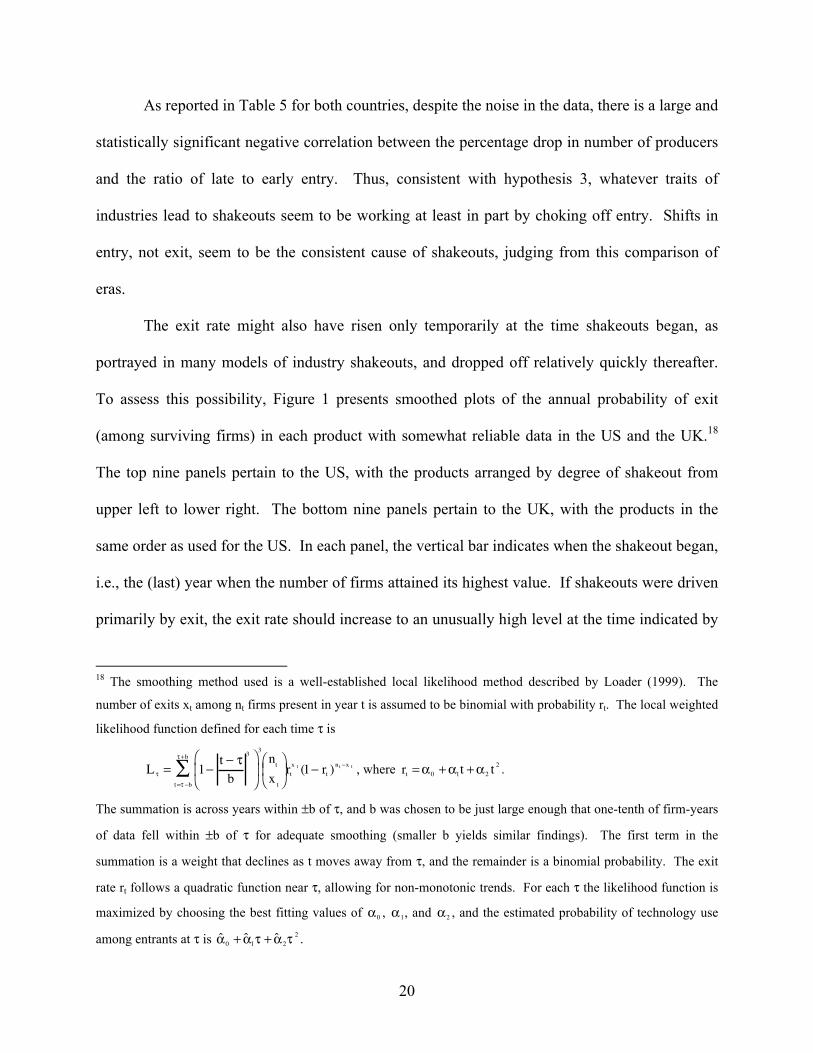
The exit rate might also have risen only temporarily at the time shakeouts began, as

portrayed in many models of industry shakeouts, and dropped off relatively quickly thereafter.

To assess this possibility, Figure 1 presents smoothed plots of the annual probability of exit

(among surviving firms) in each product with somewhat reliable data in the US and the UK.18

The top nine panels pertain to the US, with the products arranged by degree of shakeout from

upper left to lower right. The bottom nine panels pertain to the UK, with the products in the

same order as used for the US. In each panel, the vertical bar indicates when the shakeout began,

i.e., the (last) year when the number of firms attained its highest value. If shakeouts were driven

primarily by exit, the exit rate should increase to an unusually high level at the time indicated by

18 The smoothing method used is a well-established local likelihood method described by Loader (1999). The

number of exits xt among nt firms present in year t is assumed to be binomial with probability rt. The local weighted

likelihood function defined for each time τ is

�

L τ = 1−t − τb

3⎛

⎝ ⎜

⎞

⎠ ⎟

3ntx t

⎛ ⎝ ⎜

⎞ ⎠ ⎟ rt

x t (1− rt )nt −x t

t=τ −b

τ +b

∑ , where

�

rt =α0 +α1t +α2 t2 .

The summation is across years within ±b of τ, and b was chosen to be just large enough that one-tenth of firm-years

of data fell within ±b of τ for adequate smoothing (smaller b yields similar findings). The first term in the

summation is a weight that declines as t moves away from τ, and the remainder is a binomial probability. The exit

rate rt follows a quadratic function near τ, allowing for non-monotonic trends. For each τ the likelihood function is

maximized by choosing the best fitting values of

�

α0 ,

�

α1, and

�

α2 , and the estimated probability of technology use

among entrants at τ is

�

ˆ α 0 + ˆ α 1τ + ˆ α 2τ2 .

21

the bar. This apparently did occur in a few of the products in each country: tires, typewriters,

and perhaps cathode ray tubes in the US, and cathode ray tubes, electric blankets, and perhaps

adding and calculating machines in the UK. Yet the exit rate was not unusually high in just as

many cases: television sets, adding and calculating machines, and electric blankets in the US,

and tires, television sets, and typewriters in the UK. Thus the evidence suggests that price wars,

new technologies, or other events sometimes contributed to shakeouts by raising the probability

of exit, but a decrease in entry always contributed to any substantial shakeout. Indeed, in

products with strong shakeouts, the drop-offs in entry per annum were multiplicatively much

larger than the increases in probability of exit, and as often as not shakeouts were caused solely

by the drop-off in entry.

Hypothesis 4 indicates that late entrants are more likely to exit than early entrants in

industries with shakeouts, but that this characteristic does not pertain in industries without

shakeouts. To test this hypothesis, again a mechanism is needed to classify which firms are early

and late, and again the simplest division is chosen to avoid subjectivity. Firms within each

country and product were rank-ordered by date of entry, and the first 50% of firms were

classified as early entrants, except for any firms entering in the year with the 50th percentile.

Firms entering in that year and later were classified as late entrants. To examine impacts on exit,

probit models were estimated for the full sample of products. The models took the form:

Pr[Exitpcit ] = Φ(β0p +β1pukc +β2Spct +β3Lpct + ′γ ait + ...) , (1)

where Pr[Exitpcit ] is the probability of exit (conditional on the regressors) for firm i in year t

producing product p in country c, Φ(⋅) is the cumulative normal distribution function,

�

ukc is a

dummy variable equal to 0 in the US or 1 in the UK,

�

Spct equals 1 during the first decade after

the peak in an industry’s number of firms or 0 at other times,

�

L pct equals 1 at times ten or more

22

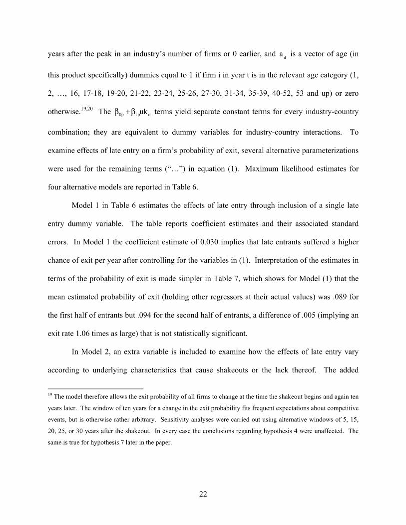
years after the peak in an industry’s number of firms or 0 earlier, and a it is a vector of age (in

this product specifically) dummies equal to 1 if firm i in year t is in the relevant age category (1,

2, …, 16, 17-18, 19-20, 21-22, 23-24, 25-26, 27-30, 31-34, 35-39, 40-52, 53 and up) or zero

otherwise.19,20 The

�

β0p +β1pukc terms yield separate constant terms for every industry-country

combination; they are equivalent to dummy variables for industry-country interactions. To

examine effects of late entry on a firm’s probability of exit, several alternative parameterizations

were used for the remaining terms (“…”) in equation (1). Maximum likelihood estimates for

four alternative models are reported in Table 6.

Model 1 in Table 6 estimates the effects of late entry through inclusion of a single late

entry dummy variable. The table reports coefficient estimates and their associated standard

errors. In Model 1 the coefficient estimate of 0.030 implies that late entrants suffered a higher

chance of exit per year after controlling for the variables in (1). Interpretation of the estimates in

terms of the probability of exit is made simpler in Table 7, which shows for Model (1) that the

mean estimated probability of exit (holding other regressors at their actual values) was .089 for

the first half of entrants but .094 for the second half of entrants, a difference of .005 (implying an

exit rate 1.06 times as large) that is not statistically significant.

In Model 2, an extra variable is included to examine how the effects of late entry vary

according to underlying characteristics that cause shakeouts or the lack thereof. The added

19 The model therefore allows the exit probability of all firms to change at the time the shakeout begins and again ten

years later. The window of ten years for a change in the exit probability fits frequent expectations about competitive

events, but is otherwise rather arbitrary. Sensitivity analyses were carried out using alternative windows of 5, 15,

20, 25, or 30 years after the shakeout. In every case the conclusions regarding hypothesis 4 were unaffected. The

same is true for hypothesis 7 later in the paper.

23

variable is an interaction term, the late entry dummy multiplied by the fractional drop in number

of firms that occurred in the relevant country and industry, as reported in Table 1. (Both

variables have already been included singly in Model 1; the fractional drop is implicitly included

as its effects are absorbed by the

�

β0p +β1pukc terms.) When the additional term is included, it

becomes apparent that there is a strong early mover advantage in products with strong shakeouts,

but an early mover disadvantage in products with no shakeouts. From the top panel of Table 7,

in a product with no shakeout, %drop=0, the probability of exit would be .077 for early entrants

versus .055 for late entrants, but in a product with an extreme shakeout, using the limiting case

where %drop=100, the probability of exit would be .094 for early entrants versus .128 for late

entrants. Both differences are significant at the .001 level, as apparent in the second panel of

Table 7, and the difference (.055-.077)-(.128-.094) is also significant at the .001 level.

Because the dependent variable, exit, determines together with entry the number of

companies in each year, the variable %drop is endogenous. Therefore in Models 3 and 4 the

endogenous variable Late x % Drop / 100 is instrumented, by replacing %drop with the other

country’s %drop in number of firms, a highly correlated variable that is not affected by the

dependent variable. In Model 3 the other country’s %drop is computed using only years

preceding substantial international trade, and in Model 4 the other country’s %drop is computed

using all years. Maximum likelihood estimates of instrumental variables probit models are

reported in the columns of Table 6 denoted Model 3 and Model 4, and corresponding predicted

probabilities are reported in Table 7. In both models, use of the instrumental variables does not

alter the conclusions: early entrants are estimated to have had the same advantage given a severe

20 The omitted age category is 0. Age categories were chosen by grouping together successive integer ages the

minimum amount necessary to achieve standard errors less than 0.1 on all age coefficients except the last (for which

the standard error was just over 0.1) in a typical model.

24

shakeout, and the same disadvantage given zero shakeout. In both cases a Wald test of

exogeneity fails to reject the null hypothesis that Late x % Drop / 100 is exogenous. The

explanation for this apparent exogeneity is that variations in exit in fact sometimes increase and

sometimes decrease the degree of shakeout depending on whether exit occurs before or after the

peak in the number of firms, and that after all variations in entry not exit are the primary

determinant of the degree of shakeout.

In Model 5 the degree of early mover advantage is estimated using a separate coefficient

for each product. The estimates show a fair degree of variation between products in the degree

of early mover advantage, and again a strong correlation is clearly present between severity of

shakeout and estimated early mover advantage. The four products with the most severe

shakeouts have higher hazards for later entrants, as can readily be observed at the bottom of

Table 7, although the difference is small for adding and calculating machines. For the three

other products the differences are all statistically significant at conventional levels. In Model 6,

the product level coefficients of early mover advantage are augmented with interaction terms to

test to what degree early mover advantage in the UK differed from that in the US. The estimates

for these interaction terms in Table 6 tend to be near zero and statistically insignificant,

suggesting that quite similar dynamic processes of competition were at work in both countries.

The table reports estimated time period effects: the hazard is estimated to be somewhat

higher on average in the decade following the peak in the number of firms, labeled “Shakeout

Decade,” than in earlier years. In the “Later Eras” of the industries, the probability of exit

apparently declined on average toward pre-shakeout values. Thus, even with controls for time

effects, business age, and inter-industry differences, there is a robust relationship between the

25

degree of industry shakeout and the increased exit probability of relatively late entrants,

consistent with hypothesis 4.

C. Technology and Industry Dynamics

To test hypothesis 5, the number of patents in each product were compared over the first

30 years of available data in each industry’s life cycle (beginning no earlier than the date of the

product’s first listing in the US or UK directories). Table 8 reports the resulting counts of

numbers of patents, for All patents in the first column, or for only indigenous Industry producers

in the second column.21 The figures tend to be higher for industries with more severe shakeouts,

as suggested by hypothesis 5. The logarithms of both counts of patents have a positive

correlation with the percentage drop in number of producers, in the US 0.524 (p=.15) for all

patents or 0.539 (p=.13) for indigenous producer patents, in the UK 0.636 (p=.07) for all patents

or 0.460 (p=.21) for indigenous producer patents. Although the measures are clouded by both

random errors in the data and cross-industry differences in the propensity to patent, this provides

suggestive evidence of a relationship between severity of shakeout and R&E activity.

To test hypothesis 6, firms are divided into early and late entrants as in the previous

section, and the mean number of patents per year, during years when firms are producing, is

computed for each group.22 The last three columns of Table 8 report the results. In the

industries with severe shakeouts, typewriters, tires, television sets, cathode ray tubes, and adding

21 No attempt was made to control for possible differences in the propensity to patent over time, although the data in

Table 7 are suggestive that products in later years may have had somewhat greater rates of patenting relative to

earlier years. 22 In case the number of patents granted per year is biased because some firms received patents only after exit, an

alternative measure was computed counting patents granted during the years firms produced plus the ten years after

exit, and dividing by the number of years produced. In fact, presumably because firms predicted by the theory to

carry out R&E were most active at R&E-related patenting, use of this measure only strengthened the conclusions.

26

and calculating machines, the early producers have substantially higher numbers of patents per

year than late producers. This finding agrees with hypothesis 6. As expected, for most of the

other products the tiny number of patents involved makes it virtually impossible to check

whether earlier and later entrants differed at all in their rates of patenting. For only one other

product, zippers, is there a substantial number of patents, and in this case the evidence suggests

that early entrants also dominated patenting; this is not anticipated by the theory for the US but

may be consistent with the theory for the UK given the 40% drop in number of producers

observed in the UK. Thus, although the low-shakeout industry of zippers is an anomaly, the

evidence confirms the prediction that early entrants dominate R&E activity in industries with

strong shakeouts.23

Hypothesis 7 indicates that successful R&E activity should reduce the probability of exit

in industries with strong shakeouts, but less so in industries with little or no shakeout. To test

this hypothesis, probit models of exit were estimated similar to Model 2 reported earlier, but

using only the years 1920 onward, when patent data are available. In Table 9, which reports the

estimates, Model 7 is the direct analogue of Model 2. Similarly to the earlier exit models, late

entrants are estimated to have the advantage of a 0.020 lower exit rate in industries without

shakeouts, but the strong disadvantage of a 0.039 higher exit rate in industries with strong

shakeouts (see Table 10; both differences, and the difference between them, are significant at the

.001 level).

In Model 8, two R&E-related variables are added: a 1-0 dummy equal to 1 if firm i

accomplished R&E recently as judged by whether the firm received one or more patents within

the five years ending at t, and this dummy variable multiplied by the fractional drop in the

23 These results must be interpreted with caution as they are sensitive to any errors in classification of firms

27

number of firms (recall that the fractional drop itself is also implicitly included in Model 7 as its

effects are entirely absorbed by the industry dummies). With the R&E-related variables

included, the estimated effect of Late x % Drop / 100 falls slightly, as one would expect on

inclusion of a crude control for the source of late-entry disadvantage in strong-shakeout

industries. More importantly, the estimates indicate that R&E-related patenting enormously

reduced the probability of exit, but only in products with substantial shakeouts. Patenting in

non-shakeout industries is estimated to have decreased the probability of exit from .066 to .042

(a decrease significant at the .01 level), a decrease of 36%. In contrast, patenting in industries

with severe shakeouts (approaching a 100% drop in number of firms) is estimated to have

decreased the probability of exit from .119 to .053, a decrease of 55%. The difference between

non-shakeout and severe-shakeout industries is statistically significant at the .05 level when

considering the absolute, but not the percentage, decreases in probabilities. The findings are

robust to instrumentation of %drop with the other nation’s %drop in the interaction with

patenting, in years preceding strong international trade in Model 9 or all years in Model 10, and

Wald tests of exogeneity fail to find any sign of endogeneity. Thus the evidence is at least

weakly consistent with hypothesis 7, indicating an especially strong role for R&E (excluding

new product development) in industries that experience strong shakeouts.

5. Conclusion

This paper has analyzed whether industry dynamics typically stem from industry-specific

traits. A theoretical view described in this paper implies distinctive testable hypotheses, used to

guide a search for correlations in patterns of industry dynamics. Moreover, inter-country

comparisons of industry dynamics, comparing nations where a non-trivial industry was

regarding whether they originated as indigenous or foreign producers.

28

established early, provide a means to assess whether some underlying traits yield highly

predictable patterns of industry dynamics.

First, counts of the number of firms over time were compared between the US and the

UK in matched, narrowly defined product industries. The counts show surprising regularity

despite noise in the data. Products with severe shakeouts in one country had severe shakeouts in

the other country, and vice versa, with the degree of shakeout often nearly identical across the

two nations. The year when the number of firms reached its peak also was similar across

countries.

Second, entry and exit patterns were compared across product industries with varying

degrees of shakeouts. According to the theoretical view described, entry should decline – and

the rate of exit need not increase – around the time of an industry’s shakeout, but only if an

industry experienced a substantial shakeout. Likewise earlier entrants into an industry should

have a substantial advantage over later entrants, resulting in a lower rate of exit, but again only in

industries with substantial shakeouts. The patterns should hold similarly across different

national markets. All these patterns were confirmed using extensive, novel data on producers’

entry and exit times in narrowly-defined product markets in the US and UK.

Third, to confirm the plausibility of research and engineering as the driving force behind

the inter-industry differences, UK patent data from as early as the 1920s to recent years were

collected, culled to focus on research and engineering of the existing product rather than new

product development, and matched to the firm data in this study. Despite inter-industry

differences in the propensity to patent, industries with substantial shakeouts seem to have had

greater innovative opportunity. More importantly, relatively early entrants in industries with

severe shakeouts had the greatest concentration of innovative output. Successful innovation

29

coincided with greatly reduced probabilities of firm exit, in the near-term future, but only in

industries with extreme shakeouts.24

Of course other product and market characteristics could also yield firm advantage and

act in a similar manner; the tests in this paper and in Klepper and Simons (1997, 2000a, 2005)

primarily confirm the important role of technological advance as a driving force in industry

dynamics. For example, Sutton (1991) shows that advertising-intensive food product industries

experience a high lower bound to their degree of concentration, and interprets the finding as

evidence that advertising not technology is responsible for these industries’ high lower bound to

concentration. However, tests of the role of advertising and of distribution networks in selected

industries with extreme shakeouts indicate that these factors either had little relation to

competitive success or had effects independent of a stronger effect of technological advance

(Klepper and Simons 2000a, 2000b). This suggests both that the role of technological change is

particularly important in causing shakeouts, and that the estimated effects of technological

change are not merely spurious correlation.

The tests carried out here are distinctive as regards many theories of industry dynamics.

In contrast to event-based shakeout theories, in which a single event such as the advent of a new

technology (Jovanovic and MacDonald, 1994) or the formation of a dominant product standard

(Utterback and Suárez, 1993), exit did not necessarily rise at the time of a shakeout. Further

evidence that individual events do not ordinarily cause shakeouts is available in Klepper and

Simons (1997, 2000a, 2005).25 Demand contraction is not the typical cause (although slowing

24 Similarly a few studies of cross-industry characteristics including Agarwal (1998) suggest that unique underlying

technological characteristics pertain to industries with shakeouts. 25 Theories of competence-destroying and disruptive technologies if applied to shakeouts likewise imply temporary

increases in exit rate, so do not explain typical industry shakeouts (Foster, 1986; Tushman and Anderson, 1986;

Anderson and Tushman, 1990; Henderson and Clark, 1990; Schnaars, 1994; Christensen and Rosenbloom, 1995).

30

growth rates may still contribute), as demonstrated in many studies including Gort and Klepper

(1982). Theories of overentry as in Camerer and Lovallo (1999) imply a market correction after

which exit rates return to lower levels, and hence are likewise inconsistent with the sustained

high exit rates observed here and in Klepper and Miller (1995). In contrast Klepper and Simons

(1997, 2000a, 2000b, 2005) and Klepper (2002) present evidence consistent with the theoretical

here, in which shakeouts result from cessation of entry and continued exit (under pressure of

declining profit) due to gradual solidification of leading firms’ market leadership caused by

cumulating relative advantage related to product and process innovation.

The empirical results in this paper provide the first independent confirmation of the

findings of Gort and Klepper (1982) that over the industry life cycle, products commonly

experience a growth and then substantial decline in their number of producers. They also

confirm, as one may read from the Gort-Klepper analysis, that seemingly not all industries

experience substantial shakeout. In fact the results shown here confirm using an independent

data source the extent and timing of industry shakeouts in 18 of the 46 industries in their sample.

This finding goes beyond confirmation of the conclusion that shakeouts frequently but not

always occur in industries, and moreover suggests that there is some underlying characteristic

associated with specific products that yields similar industry dynamics across different countries.

Shakeout in some industries but not others is an indicated feature of theories by

Jovanovic and MacDonald (1994) theory and several others, but is not considered in the theories

by Klepper (1996, 2002) that are central to the theoretical view herein. Indeed, the simple

extension theorized here, such that some industries experience little or no shakeout because of

underlying technological opportunities, can be seen as an important philosophical break in which

the decision is made to study why many industries do not experience substantial industry

31

shakeouts in order both to understand the phenomenon of shakeouts and to explain outcomes

more fully across typical industries. The approach here is in many ways close in spirit to

Sutton’s (1991, 1998) static analyses of how an underlying characteristic causes concetration in

some product industries but not others.

The empirical findings show that early-mover advantage is systematically tied up with

the degree of industry shakeouts. This finding is not tautological, for late-mover advantages, or

exogenous events that affect all firms alike, could also cause industry shakeouts.26 The

interaction between early-mover advantage and shakeout is a predictable pattern that can extend

understanding and tests of the source and role of early-entry advantages. The marriage that

Lieberman and Montgomery (1998) sought to broker, between literatures on first-mover

advantage and resource-based views of the firm, needs to be extended to a trinity of early-mover

advantage, firm resources, and long-run industry dynamics. The present study suggests a way

forward to better understand in what situations and why early-mover advantages should arise.

Understanding the most important causes of industry dynamics is a key challenge for

researchers. Although this challenge is difficult, it is extremely important, because it is requisite

for in-depth understanding of why certain industries become concentrated among few producers,

of market success or failure for a large fraction of businesses, and of the related societal impacts

stemming from product quality improvement and cost reduction. As the present study helps to

26 However, early-mover advantages can be a cause of shakeouts, as theorized here. For example if entrants entering

at rate e1 per year in times 0 to t1 have constant exit hazard r1 forever, and entrants after t1 enter at a constant rate e2

per year and have constant exit hazard r2>r1 forever, then it is easy to derive that the eventual %drop in number of

firms is 0 if n1(t1) ≡

e1

r1(1− e− r1t1 ) ≤

e2

r2

but otherwise is (100%) ⋅

n1(t1)− (e2 / r2 )n1(t1)

≅ (100%) ⋅(e1 / r1)− (e2 / r2 )

(e1 / r1) where

the approximation is close if the first-period number of firms approaches by t1 its steady-state value of e1 / r1 and in

any case the right hand side is an upper bound on the %drop.

32

show, the nature of technological change appears to be an important characteristic underlying

industry competitive dynamics. Industries with shakeouts, in particular, appear to demand from

their participants the rapid development of unusually large numbers of relatively incremental

innovations. This form of innovation being one of the key means to improvement in consumer

welfare and productivity, it appears that the dependence of shakeout and non-shakeout industry

dynamics on innovation is a central factor involved in shaping economic growth.

References

Abernathy, William J. and James M. Utterback. “Patterns of Industrial Innovation.” Technology

Review 80, June/July 1978, pp. 41-47.

Adler, Michael. Antique Typewriters: From Creed to QWERTY. Schiffer Books, 1997.

Agarwal, Rajshree. “Evolutionary Trends of Industry Variables.” International Journal of

Industrial Organization 16, 1998, pp. 511-525.

Anderson, Philip and Michael L. Tushman. “Technological Discontinuities and Dominant

Designs: A Cyclical Model of Technological Change.” Administrative Science Quarterly 35,

1990, pp. 604-633.

Arnold, Erik. Competition and Technological Change in the Television Industry: An Empirical

Evaluation of Theories of the Firm. London: Macmillan Press, 1985.

Bain, Joe S. International Differences in Industrial Structure. New Haven, CT: Yale University

Press, 1966.

Bartelsman, Eric J., and Wayne B. Gray. “The NBER Productivity Database.” NBER Technical

Working Paper no. 205, October 1996.

Camerer, Colin and Dan Lovallo. “Overconfidence and Excess Entry: An Experimental

Approach,” American Economic Review 89 (1), March 1999, pp. 306-318.

33

Carlip, Alfred Benjamin. The Slide Fastener Industry: A Study of Market Structure and

Innovation. PhD dissertation, Columbia University, 1960.

Christensen, Clayton M. and Richard S. Rosenbloom. “Explaining the Attacker's Advantage:

Technological Paradigms, Organizational Dynamics, and the Value Network.” Research

Policy 24, 1995, pp. 233-257.

Feenstra, Robert C. “NBER Trade Database, Disk1: U.S. Imports, 1972-1994: Data and

Concordances.” NBER Working Paper no. 5515, March 1996.

Flaherty, M. Therese. “Industry Structure and Cost-Reducing Investment.” Econometrica 48,

1980, pp. 1187-1209.

Foster, Richard N. Innovation: The Attacker’s Advantage. New York: Summit Books, 1986.

Frederiksen, Peter Carl. “Prospects of Competition from Abroad in Major Manufacturing

Industries: Case Studies of Flat Glass, Primary Aluminum, Typewriters, and Wheel Tractors.”

PhD dissertation, Washington State University, 1974.

Gort, Michael and Steven Klepper. “Time Paths in the Diffusion of Product Innovations.”

Economic Journal 92, 1982, pp. 630-653.

Gostony, Henry and Stuart Schneider. The Incredible Ball Point Pen. Schiffer Books, 1998.

Henderson, Rebecca M. and Kim B. Clark. “Architectural Innovation: The Reconfiguration of

Existing Product Technologies and the Failure of Established Firms.” Administrative Science

Quarterly 35, 1990, pp. 9-30.

Jovanovic, Boyan and Glenn MacDonald. “The Life Cycle of a Competitive Industry.” Journal

of Political Economy, April 1994, 102 (2), pp. 322-347.

King, Algin Braddy. The Marketing of Phonograph Records in the United States: An Industry

Study. PhD dissertation, Ohio State University, 1966.

34

Klepper, Steven. “Entry, Exit, Growth, and Innovation over the Product Life Cycle.” American

Economic Review 86 (3), June 1996, pp. 562-583.

Klepper, Steven. “Firm Survival and the Evolution of Oligopoly.” RAND Journal of Economics

33 (1), 2002, pp. 37-61.

Klepper, Steven, and Elizabeth Graddy. “The Evolution of New Industries and the Determinants

of Market Structure.” RAND Journal of Economics 21, 1990, pp. 27-44.

Klepper, Steven, and John H. Miller. “Entry, Exit and Shakeouts in the United States in New

Manufactured Products.” International Journal of Industrial Organization 13, 1995, pp. 567-

591.

Klepper, Steven, and Kenneth L. Simons. “Technological Extinctions of Industrial Firms: An

Enquiry into their Nature and Causes.” Industrial and Corporate Change 6, 1997, pp. 379-

460.

Klepper, Steven, and Kenneth L. Simons. “The Making of an Oligopoly: Firm Survival and

Technological Change in the Evolution of the U.S. Tire Industry.” Journal of Political

Economy 108, 2000a, pp. 728-760.

Klepper, Steven, and Kenneth L. Simons. “Dominance by Birthright: Entry of Prior Radio

Producers and Competitive Ramifications in the U.S. Television Receiver Industry,” Strategic

Management Journal 21 (10-11), October-November 2000b, pp. 997-1016.

Klepper, Steven, and Kenneth L. Simons. “Industry Shakeouts and Technological Change,”

International Journal of Industrial Organization 23 (1-2), February 2005, pp. 23-43.

Lieberman, Marvin B., and David B. Montgomery. “First-Mover (Dis)advantages:

Retrospective and Link with the Resource-Based View. Strategic Management Journal 19,

1998, pp. 1111-1125.

35

Loader, Clive. Local Regression and Likelihood. New York: Springer, 1999.

Lundvall, B.-Å., ed. National Systems of Innovation: Towards a Theory of Innovation and

Interactive Learning. London: Pinter, 1992.

Mansfield, Edwin. Industrial Research and Technological Innovation. New York: Norton,

1968.

Martin, Ernst. Die Rechenmaschinen und ihre Entwicklungsgeschichte (The Calculating

Machines: Their History and Development). Pappenheim: Johannes Mayer, 1925. Translation

by Peggy Aldrich Kidwell and Michael R. Williams, Cambridge, Mass. and Los Angeles: MIT

Press and Tomash Publishers, 1992.

McGahan, Anita M. and Brian S. Silverman. “How Does Innovative Activity Change as

Industries Mature?” International Journal of Industrial Organization 19, 2001, pp. 1141-1160.

Nelson, Richard R., ed. National Innovation Systems. New York: Oxford University Press,

1993.

Penrose, Edith. The Theory of the Growth of the Firm. Oxford: Basil Blackwell, 1959.

Petrakis, Emmanuel, Eric Rasmusen, and Santanu Roy, “The Learning Curve in a Competitive

Industry,” RAND Journal of Economics 28(2), (1997), pp. 248-268.

Pryor, Frederic L. “An International Comparison of Concentration Ratios.” Review of

Economics and Statistics 54 (2), May 1972, pp. 130-140.

Schmalensee, Richard. “Inter-Industry Studies of Structure and Performance.” In Richard

Schmalensee and Robert D. Willig, eds., Handbook of Industrial Organization, Volume 2,

Amsterdam: Elsevier, 1989, pp. 951-1009.

Schnaars, Steven P. Managing Imitation Strategies: How Later Entrants Seize Markets from

Pioneers. Free Press (Macmillan), 1994.

36

Shaked, Avner and John Sutton. “Product Differentiation and Industrial Structure.” Journal of

Industrial Economics 36 (2), 1987, pp. 131-146.

Sutton, John. Sunk Costs and Market Structure: Price Competition, Advertising, and the

Evolution of Concentration. Cambridge, Mass.: MIT Press, 1991.

Sutton, John. Technology and Market Structure: Theory and History. Cambridge, Mass.: MIT

Press, 1998.

Tushman, Michael L., and Philip Anderson. “Technological Discontinuities and Organizational

Environments.” Administrative Science Quarterly 31, 1986, pp. 439-465.

U.S. Department of Commerce, International Trade Administration. “Radio Communication and

Detection Equipment.” In U.S. Industrial Outlook 1991, Washington, D.C.: U.S. Department

of Commerce, 1991.

Utterback, James and William J. Abernathy. “A Dynamic Model of Product and Process

Innovation.” Omega 3 (6), 1975, pp. 639-656.

Utterback, James and Suárez, Fernando. “Innovation, Competition, and Industry Structure.”

Research Policy, 1993, 22, pp. 1-21.

Willer, Paul. Whose Zip? A History of the Zip and the Lightning/Opti Group. Enderby: Opti,

1994.

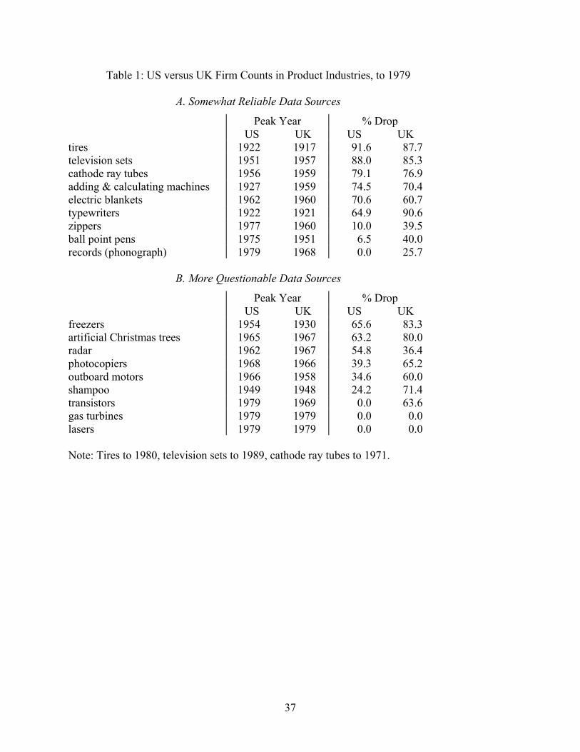
37

Table 1: US versus UK Firm Counts in Product Industries, to 1979

A. Somewhat Reliable Data Sources

Peak Year % Drop US UK US UK tires 1922 1917 91.6 87.7 television sets 1951 1957 88.0 85.3 cathode ray tubes 1956 1959 79.1 76.9 adding & calculating machines 1927 1959 74.5 70.4 electric blankets 1962 1960 70.6 60.7 typewriters 1922 1921 64.9 90.6 zippers 1977 1960 10.0 39.5 ball point pens 1975 1951 6.5 40.0 records (phonograph) 1979 1968 0.0 25.7

B. More Questionable Data Sources

Peak Year % Drop US UK US UK freezers 1954 1930 65.6 83.3 artificial Christmas trees 1965 1967 63.2 80.0 radar 1962 1967 54.8 36.4 photocopiers 1968 1966 39.3 65.2 outboard motors 1966 1958 34.6 60.0 shampoo 1949 1948 24.2 71.4 transistors 1979 1969 0.0 63.6 gas turbines 1979 1979 0.0 0.0 lasers 1979 1979 0.0 0.0 Note: Tires to 1980, television sets to 1989, cathode ray tubes to 1971.

38

Table 2: Sample Characteristics for US and UK Firm Counts

A. Somewhat Reliable Data Sources

First Year of Data Peak Number US UK US UK tires 1905 1896 274 106 television sets 1947 1935 92 34 cathode ray tubes 1949 1950 67 13 adding & calculating machines 1905 1910 51 27 electric blankets 1915 1941 17 28 typewriters 1905 1903 37 32 zippers 1928 1933 80 38 ball point pens 1946 1948 108 20 records (phonograph) 1905 1913 47 35

B. More Questionable Data Sources

First Year of Data Peak Number US UK US UK freezers 1944 1915 61 6 artificial Christmas trees 1924 1949 19 5 radar 1945 1951 168 11 photocopiers 1939 1954 28 23 outboard motors 1909 1930 26 10 shampoo 1905 1939 128 14 transistors 1952 1959 72 11 gas turbines 1940 1948 35 13 lasers 1962 1969 106 4

C. Differences After Excluding Years with Substantial International Trade

Country Peak Year % Drop Peak Number television sets US 64.1 television sets UK 64.7 adding & calculating machines US 51.0 adding & calculating machines UK 1958 0.0 typewriters UK 62.5 zippers US 1972 0.0 48 zippers UK 34.2 artificial Christmas trees both excluded transistors US 1963 26.9 67 transistors UK 0.0 lasers both excluded

39

Table 3: Correlation Coefficients Across Countries

A. Somewhat Reliable Data Sources

All Years Excluding Years after Substantial Trade

peak year 0.735 * 0.749 * peak year – min.(first year) 0.694 * 0.715 * first year of data 0.849 ** 0.849 ** % drop 0.923 *** 0.679 * peak number 0.872 ** 0.858 **

B. More Questionable Data Sources

All Years Excluding Years after Substantial Trade

peak year 0.836 ** 0.803 * peak year – min.(first year) 0.780 * 0.771 * first year of data 0.507 0.360 % drop 0.652 † 0.627 peak number -0.105 -0.202

C. All Data Sources

All Years Excluding Years after Substantial Trade

peak year 0.772 *** 0.749 *** peak year – min.(first year) 0.718 *** 0.728 ** first year of data 0.734 *** 0.706 ** % drop 0.769 *** 0.625 ** peak number 0.626 ** 0.632 ** Note: † p<.10, * p<.05, ** p<.01, *** p<.001 (2-tailed t-test)

40

Table 4: Early-Era Versus Late-Era Entry and Exit by Product, US and UK

A. Somewhat Reliable Data Sources

Late/Early Entry Late/Early Exit US UK US UK tires 0.097 *** 0.093 *** 2.329 *** 1.534 ** television sets 0.039 † 0.159 * 1.014 0.862 cathode ray tubes 0.078 * 0.428 0.883 0.779 adding & calculating machines 0.380 ** 1.110 1.329* 1.199 electric blankets 0.150 ** 0.676 0.838 0.222 *** typewriters 0.732 0.490 ** 1.054 1.118 zippers 1.292 0.578 † 1.015 1.005 ball point pens 0.758 0.294 * 1.059 2.865 *** records (phonograph) 0.888 1.345 1.609 ** 2.200 ***

B. More Questionable Data Sources

Late/Early Entry Late/Early Exit US UK US UK freezers 0.206 *** 1.000 0.830 0.880 artificial Christmas trees 0.769 0.747 0.178 *** 0.444 radar 0.330 *** 0.529 0.785* 2.407 * photocopiers 0.797 0.410 * 0.464 ** 0.458 * outboard motors 1.194 0.952 0.749 0.327 † shampoo 0.788 0.667 1.005 1.620 transistors 0.925 0.222 ** 1.694 * 1.128 gas turbines 0.859 1.875 0.793 1.460 lasers 0.836 5.000 † 0.876 0.000 Note: † p<.10, * p<.05, ** p<.01, *** p<.001 (entry: 2-tailed t-test for equality of means, with variance allowed to differ, between periods; exit: 2-tailed Wald test of H0: β1=0 in maximum likelihood probit regressions of exit on a constant term and the LateEra dummy, with cluster-robust (by firm) variance estimation; for exit in lasers in the UK, exact logistic regression is used to assess statistical significance since probit regression is incapable of parameter estimation for an independent variable whose value perfectly predicts exit).

41

Table 5: Entry and Exit Correlation Coefficients

A. Somewhat Reliable Data Sources

All Years Excluding Years after Substantial Trade

% drop and entry ratio, US -0.867 ** % drop and entry ratio, UK -0.551 entry ratio US and UK 0.373 0.635 † % drop and exit ratio, US 0.113 % drop and exit ratio, UK -0.507 exit ratio US and UK 0.327 0.154

B. More Questionable Data Sources

All Years Excluding Years after Substantial Trade

% drop and entry ratio, US -0.585 † % drop and entry ratio, UK -0.728 * entry ratio US and UK 0.126 0.129 % drop and exit ratio, US -0.606 † % drop and exit ratio, UK -0.064 exit ratio US and UK 0.281 0.204

C. All Data Sources

All Years Excluding Years after Substantial Trade

% drop and entry ratio, US -0.800 *** % drop and entry ratio, UK -0.674 ** entry ratio US and UK 0.243 0.472 † % drop and exit ratio, US 0.018 % drop and exit ratio, UK -0.188 exit ratio US and UK 0.388 0.291 Note: † p<.10, * p<.05, ** p<.01, *** p<.001 (2-tailed t-test)

42

Table 6: Probit and IV Probit Regressions of Firm Exit, Maximum Likelihood Estimates

Dependent variable: Exit (1=exited in year t, 0=survived) (1) (2) (3) (4) (5) (6) Probit Probit IV Probit IV Probit Probit Probit Late entry effects: Late Entry 0.030 -0.198*** -0.208** -0.226*** (0.028) (0.049) (0.063) (0.053) Late x % Drop / 100 § 0.377*** 0.397*** 0.430*** (0.067) (0.097) (0.076) by product: Late x Tires 0.098* 0.157** (0.042) (0.052) Late x Television sets 0.254*** 0.299*** (0.064) (0.076) Late x Cathode ray tubes 0.341*** 0.335*** (0.092) (0.101) Late x Adding & calc. 0.046 0.115 (0.072) (0.083) Late x Electric blankets -0.127 -0.266* (0.094) (0.128) Late x Typewriters 0.126 0.019 (0.092) (0.107) Late x Zippers -0.158* -0.222* (0.079) (0.100) Late x Ball point pens -0.141* -0.095 (0.069) (0.078) Late x Records -0.174** -0.080 (0.066) (0.085) by product in UK: Late x Tires x UK -0.140† (0.075) Late x Television sets x UK -0.148 (0.139) Late x Cathode ray tubes x UK 0.028 (0.240) Late x Adding & calc. x UK -0.300* (0.146) Late x Electric blankets x UK 0.252 (0.183) Late x Typewriters x UK 0.290 (0.180) Late x Zippers x UK 0.173 (0.159) Late x Ball point pens x UK -0.203 (0.169) Late x Records x UK -0.211 (0.134)

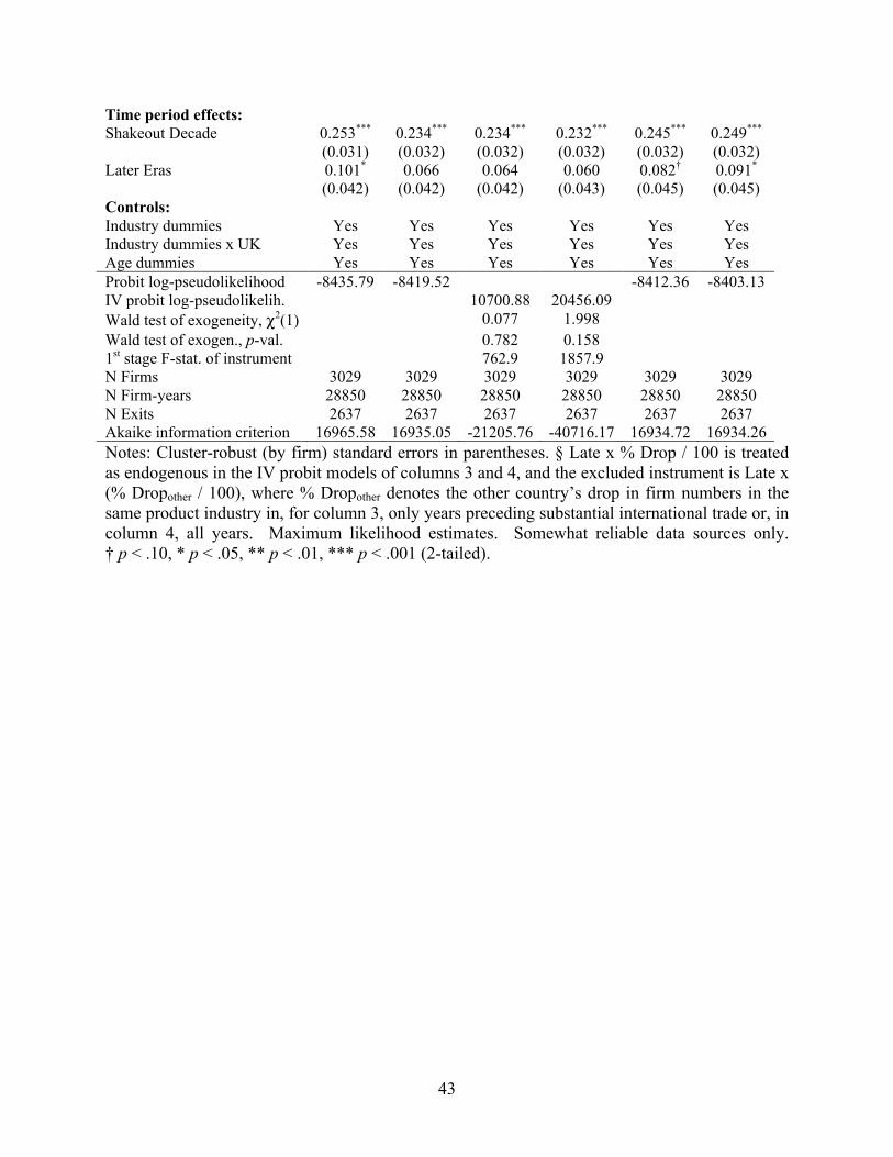
43

Time period effects: Shakeout Decade 0.253*** 0.234*** 0.234*** 0.232*** 0.245*** 0.249*** (0.031) (0.032) (0.032) (0.032) (0.032) (0.032) Later Eras 0.101* 0.066 0.064 0.060 0.082† 0.091* (0.042) (0.042) (0.042) (0.043) (0.045) (0.045) Controls: Industry dummies Yes Yes Yes Yes Yes Yes Industry dummies x UK Yes Yes Yes Yes Yes Yes Age dummies Yes Yes Yes Yes Yes Yes Probit log-pseudolikelihood -8435.79 -8419.52 -8412.36 -8403.13 IV probit log-pseudolikelih. 10700.88 20456.09 Wald test of exogeneity, χ2(1) 0.077 1.998 Wald test of exogen., p-val. 0.782 0.158 1st stage F-stat. of instrument 762.9 1857.9 N Firms 3029 3029 3029 3029 3029 3029 N Firm-years 28850 28850 28850 28850 28850 28850 N Exits 2637 2637 2637 2637 2637 2637 Akaike information criterion 16965.58 16935.05 -21205.76 -40716.17 16934.72 16934.26 Notes: Cluster-robust (by firm) standard errors in parentheses. § Late x % Drop / 100 is treated as endogenous in the IV probit models of columns 3 and 4, and the excluded instrument is Late x (% Dropother / 100), where % Dropother denotes the other country’s drop in firm numbers in the same product industry in, for column 3, only years preceding substantial international trade or, in column 4, all years. Maximum likelihood estimates. Somewhat reliable data sources only. † p < .10, * p < .05, ** p < .01, *** p < .001 (2-tailed).

44

Table 7: Average Predicted Probabilities of Exit by Entry Time and Late-Early Differences (1) (2) (3) (4) (5) (6) Exit Probability by Entry Time If entry were early .089***

(.003) .088*** (.003)

.088*** (.003)

.088*** (.003)

.089*** (.003)

.089*** (.003)

If entry were late .094*** (.003)

.096*** (.003)

.096*** (.003)

.096*** (.003)

.095*** (.003)

.095*** (.003)

If %drop were 0 & early .077*** (.005)

.077*** (.006)

.077*** (.005)

If %drop were 0 & late .055*** (.004)

.054*** (.005)

.054*** (.004)

If %drop were 100 & early .094*** (.004)

.093*** (.004)

.093*** (.004)

If %drop were 100 & late .128*** (.006)

.129*** (.007)

.129*** (.006)

Exit Probability if Late Entrant Minus Exit Probability if Early Entrant Unadjusted .005

(.004) .008† (.004)

.008† (.005)

.009† (.005)

.007 (.005)

.006 (.005)

If %drop were 0 -.022*** (.006)

-.023** (.008)

-.023*** (.007)

If %drop were 100 .034*** (.007)

.036*** (.010)

.036*** (.008)

In Tires .018* (.008)

.018* (.008)

In Television sets .049*** (.013)

.049*** (.013)

In Adding & calc. .007 (.011)

.006 (.011)

In Cathode ray tubes .063*** (.017)

.063*** (.017)

In Electric blankets -.017 (.012)

-.017 (.012)

In Typewriters .019 (.014)

.020 (.014)

In Zippers -.017* (.008)

-.017* (.008)

In Ball point pens -.017* (.008)

-.018* (.009)

In Records -.026* (.010)

-.027** (.010)

Notes: First panel estimates are average predicted probabilities of exit. Second panel estimates are the average predicted probability of exit if each firm entered late, minus the average predicted probability of exit if each firm entered early. Both panels are means across all observations, or across producers of specific products specified in the last nine rows, substituting hypothetical values of early or late entry and of %drop. Cluster-robust (by firm) standard errors, computed by the delta method, in parentheses. Predictions with hypothetical values of %drop allow the constant term to vary with %drop, rather than by industry, by maximum likelihood estimation of models with %drop but without industry dummies. † p < .10, * p < .05, ** p < .01, *** p < .001 (2-tailed).

45

Table 8: Patents by Country and Industry

Somewhat Reliable Data Sources Only

Patents in 30 Years Patents per Year All Industry Early Late Late/Early United States tires 1345 1225 0.190 0.015 0.079 television sets 1361 1274 0.941 0.075 0.080 cathode ray tubes 3046 1687 1.737 0.231 0.133 adding & calculating machines 221 210 0.054 0.034 0.634 electric blankets 37 36 0.075 0.051 0.686 typewriters 2143 2064 0.747 0.382 0.511 zippers 645 633 0.332 0.005 0.015 ball point pens 86 80 0.014 0.008 0.596 records (phonograph) 63 62 0.033 0.007 0.199 United Kingdom tires 3018 356 0.069 0.008 0.113 television sets 3528 705 0.390 0.106 0.271 adding & calculating machines 277 9 0.045 0.018 0.402 cathode ray tubes 1087 66 0.192 0.016 0.083 electric blankets 4 0 0.000 0.009 ∞ typewriters 618 29 0.017 0.002 0.106 zippers 558 151 0.198 0.012 0.062 ball point pens 44 4 0.002 0.000 0 records (phonograph) 31 4 0.001 0.002 2.651

46

Table 9: Hazard of Exit – Probit and IV Probit Regressions of Firm Exit, Maximum Likelihood Estimates, with Effects of Patenting

Dependent variable: Exit (1=exited in year t, 0=survived)

(7) (8) (9) (10) Probit Probit IV Probit IV Probit Late entry effects: Late Entry -0.191*** -0.197*** -0.203*** -0.194*** (0.051) (0.051) (0.054) (0.051) Late x % Drop / 100 0.397*** 0.334*** 0.347*** 0.327*** (0.072) (0.074) (0.082) (0.075) R&E effects: Patented in previous 5 years -0.197* -0.250 -0.167 (0.100) (0.182) (0.117) Patented5 x % Drop / 100 § -0.283* -0.199 -0.329† (0.139) (0.275) (0.168) Time period effects: Shakeout Decade 0.232*** 0.255*** 0.254*** 0.256*** (0.038) (0.038) (0.038) (0.038) Later Eras 0.039 0.075 0.071 0.077 (0.049) (0.049) (0.050) (0.049) Controls: Industry dummies Yes Yes Yes Yes Industry dummies x UK Yes Yes Yes Yes Age dummies Yes Yes Yes Yes Probit log-pseudolikelihood -6830.52 -6784.42 IV probit log-pseudolikelihood 16585.34 27404.12 Wald test of exogeneity, χ2(1) 0.130 0.281 Wald test of exogeneity, p-val. 0.718 0.596 1st stage F-stat. of instrument 71.8 291.2 N Firms 2512 2512 2512 2512 N Firm-years 24017 24017 24017 24017 N Exits 2124 2124 2124 2124 Akaike information criterion 13757.05 13668.84 -32966.68 -54604.23 Notes: Cluster-robust (by firm) standard errors in parentheses. § Patented5 x % Drop / 100 is treated as endogenous in the IV probit models of columns 9 and 10, and the excluded instrument is Patented5 x (% Dropother / 100), where % Dropother denotes the other country’s drop in firm numbers in the same product industry in, for column 9, only years preceding substantial international trade or, in column 10, all years. Maximum likelihood estimates. Years before 1920, when patent data are unavailable, are excluded. Somewhat reliable data sources only. † p < .10, * p < .05, ** p < .01, *** p < .001 (2-tailed).

47

Table 10: Average Predicted Probabilities of Exit and Differences (7) (8) (9) (10) Exit Probability by Entry Time If entry were early .083***

(.003) .087*** (.003)

.087*** (.003)

.087*** (.003)

If entry were late .091*** (.003)

.088*** (.003)

.088*** (.003)

.088*** (.003)

If %drop were 0 & early .074*** (.005)

.074*** (.005)

.075*** (.006)

.074*** (.005)

If %drop were 0 & late .054*** (.004)

.053*** (.004)

.052*** (.004)

.053*** (.004)

If %drop were 100 & early .089*** (.005)

.097*** (.005)

.095*** (.006)

.096*** (.005)

If %drop were 100 & late .127*** (.006)

.122*** (.006)

.123*** (.006)

.122*** (.006)

Exit Probability if Late Entrant Minus Exit Probability if Early Entrant Unadjusted .008

(.005) .001

(.005) .001

(.005) .001

(.005) If %drop were 0 -.020**

(.006) -.021***

(.006) -.022***

(.007) -.021***

(.006) If %drop were 100 .039***

(.008) .025** (.008)

.028** (.009)

.025** (.008)

Exit Probability by Patenting If patented in 5 years .048***

(.004) .048*** (.004)

.049*** (.004)

If did not patent in 5 years .096*** (.002)

.096*** (.002)

.096*** (.002)

If %drop were 0 & patented .042*** (.008)

.034* (.014)

.041*** (.010)

If %drop were 0 & no patent .066*** (.004)

.067*** (.004)

.066*** (.004)

If %drop were 100 & patented .053*** (.006)

.059*** (.013)

.053*** (.008)

If %drop were 100 & no patent .119*** (.004)

.118*** (.005)

.119*** (.004)

Exit Probability if No Patent Minus Exit Probability if Patented Unadjusted .047***

(.005) .048*** (.005)

.047*** (.005)

If %drop were 0 .024** (.009)

.033* (.016)

.026* (.011)

If %drop were 100 .067*** (.007)

.059*** (.015)

.066*** (.009)

Notes: First and third panel estimates are average predicted probabilities of exit. Second panel estimates are the average predicted probability of exit if each firm entered late, minus the average predicted probability of exit if each firm entered early. Fourth panel estimates are the average predicted probability of exit if each firm patented (related to the product) in the previous five years, minus the average predicted probability of exit if each firm did not patent in the previous five years. All panels are means across all observations, substituting hypothetical values of early or late entry, patenting, and %drop. Cluster-robust (by firm) standard errors, computed by the delta method, in parentheses. Predictions with hypothetical values of %drop allow the constant term to vary with %drop, rather than by industry, by maximum likelihood estimation of models with %drop but without industry dummies. † p < .10, * p < .05, ** p < .01, *** p < .001 (2-tailed).

48

Figure 1. Smoothed exit rates over time by product and country.