THE 19th CHESAPEAKE SAILING YACHT SYMPOSIUM

ANNAPOLIS, MARYLAND, MARCH 2009

Assessing the Wind-Heel Angle Relationship of Traditionally-Rigged Sailing Vessels William C. Lasher and Diana R. Tinlin, The Pennsylvania State University at Erie, The Behrend College Bruce Johnson and John Womack, Co-chairs, SNAME Panel O-49 Jan C. Miles, Captain, Pride of Baltimore II Walter Rybka and Wes Heerssen, Captains, U.S. Brig Niagara ABSTRACT

A program to assess the wind-heel relationship of traditionally-rigged sailing vessels has been undertaken with the eventual goal of being able to provide sailing guidance to the masters and crews. This program uses Computational Fluid Dynamics (CFD) with full-scale experimental measurement to develop and validate a wind-heel model, as well as understand the nature of how these vessels respond to different wind situations. The CFD simulations are used to assess errors in measured wind angle and direction, and the experimental data are used to establish the CFD model uncertainty. The model has been validated against a limited set of data from Pride of Baltimore II. In some cases the agreement between the model and experimental values is excellent; in other cases there is significant error. The CFD-based model is computationally expensive, so a different approach for determining the sail forces is proposed. The experimental measurements indicate that the ship is almost never in static equilibrium, which raises questions about the validity of models based on equilibrium principles. These questions have not yet been answered and are the topic of ongoing future research.

NOTATION A sail area AW apparent wind AWA apparent wind angle AWV apparent wind velocity CD drag coefficient, D/(0.5ρV2A) CL drag coefficient, L/(0.5ρV2A) CS side force coefficient (sideways projection of CL and CD) CFD computational fluid dynamics D aerodynamic drag HA heel angle

HM heeling moment IMS International Measurement System L aerodynamic lift RANS Reynolds Averaged Navier Stokes Equation RM righting moment SLIP Stability Letter Improvement Project SLEP Stability Letter Enhancement Project TW true wind TWA true wind angle TWV true wind velocity Greek symbols ρ air density INTRODUCTION

For several hundred years wooden traditionally-rigged sailing ships were the dominant form of ocean transportation. Even though fuel power replaced sail as the primary mode of propulsion long ago, there are still many traditionally-rigged sailing vessels, often called “tall ships”, world-wide. Their rigging style can range from large square-rigged ships to small and simple fore & aft rigged vessels. Today they are used for historical preservation, youth and adult education, character development, or purely recreational reasons.

The U.S. Brig Niagara (Figure 1) and the Chesapeake Bay topsail schooner Pride of Baltimore II (Figure 2) are two different examples of these tall ships. Both are reproductions of ships used by the United States in the War of 1812 on the Great Lakes and Atlantic Ocean, respectively. The vessels are used for historical interpretation, traditional sailing skills preservation, and public sails. These vessels represent the two predominant types of tall ships of their era, primarily square rigged or fore and aft rigged. See Appendix A for additional vessel descriptions.

125

Figure 1 - Niagara

Figure 2 - Pride of Baltimore II (Courtesy of Jack McKim)

Compared to typical modern sailing vessels these traditional examples present two significant differences: 1) lower average freeboard to beam ratio (lower deck height above water relative to beam), hence smaller acceptable angles of heel to keep the decks dry while sailing, and 2) square rigged sail equipment.

The first difference of lower freeboard poses a couple of questions to the operator: 1) What sail area in what wind force will achieve a good sailing experience and still keep the edge of the deck from becoming significantly submerged? 2) What increase in apparent wind speed and angle will subject the vessel to undesirable angles of heel or the possibility of a 90 degree knockdown for the same sail area?

The second difference of square rigged sails presents an especially interesting question when one considers that traditional seamanship, both written and unwritten, teaches that the “best practice” for handling traditionally-rigged, square sail-equipped sailing vessels in open waters during an instance of rising winds is to bear off as quickly as

possible in order to bring the wind aft of the beam. This provides the crew with a vessel that remains mostly vertical while they attend to shortening sail as quickly as possible, because traditional square sail rigging is more successfully and quickly handled when the wind is from behind relative to the sails.

For those readers possessing extensive sailing experience, it should be noted that traditional sailing vessels, especially those with square rigged sails, have lower-aspect ratio sail configurations than found on modern sailing vessels. Low aspect ratio sail configurations are generally much more able to sustain increased wind from behind without causing steering control problems than high-aspect ratio sail configurations. Traditional seamanship also instructs keeping the center of effort forward while bearing off before a rising wind, i.e. one should reduce sail aft more quickly than reducing sail from forward. (One of the authors, Jan C. Miles, master for more than two decades in square topsail rigged schooners sailing waters between East Asia and Eastern Europe can attest to the much reduced risk of sail handling problems for the vessel’s crew when there is sea room and time opportunity to bear off before a breeze for the purposes of taking in sail).

As a result of these issues, the crews of traditionally-rigged vessels are very concerned about wind-heel angle stability – that is, how much sail they can safely carry to maximize performance (i.e., crew/passenger enjoyment) and still have sufficient wind-heel stability margins to remain upright under various conditions.

The problem for crews of both Niagara and Pride II is the wind-heel stability guidance provided with the U.S. Coast Guard (USCG) sailing vessel inspection does not include any vessel-specific wind-heel stability behavior information. Because of this, newly assigned crew to any of the wide variety of USCG-inspected traditional sailing vessel have no formal assistance in understanding the widely differing wind-heel stability and behavioral characteristics of their vessels. Hence, when taking command of a USCG certified traditional sailing vessel for the first time, a new captain generally cannot be assumed to possess a full understanding of the ship’s wind-heel stability characteristics as a function of wind speed and sail combination, except for the fact that she has passed the generic U.S. Coast Guard stability regulations.

One might think that a question such as what it would take to seriously endanger or capsize a traditionally rigged sailing vessel would have been answered in the historical record; after all, these vessels were around for hundreds of years and sailed through almost every imaginable condition. However, the practice of conceiving sailing vessels predates the formal science of naval architecture, hence is based on a foundation of rule of thumb experience. There is, in fact, a small body of literature

126

describing practical seamanship in traditional sailing vessels, but it is largely anecdotal and the information is spotty (for example, Harland and Myers, 1984). In many cases the information only applies to specific vessels; in some cases it is simply wrong; and in most cases there is no wind-heel stability behavior described.

Interestingly, the captains of these two vessels (Walter Rybka of Niagara and Jan Miles of Pride of Baltimore II) independently approached two of the authors about collaborative studies to improve operator knowledge of traditional sailing vessel wind-heel stability. These studies resulted in two separate presentations at the previous Chesapeake Sailing Yacht Symposium (CSYS, Lasher et. al., 2007, and Miles et. al, 2007). Lasher et. al. described the development of a CFD-based model to predict the heeling moment and applied it to a study of Niagara, and Miles et. al. described an experimental program to measure and record the wind conditions and heel angle on Pride of Baltimore II. Due to their common interest and a clear need to learn more about the wind-heel stability of traditionally-rigged vessels, the authors decided to work together on a unified program.

This paper presents an overview of this program as well as some preliminary results. The new program is a further development of the previous CFD model, along with experimental verification through enhanced full-scale testing. The previously published work of the authors will first be summarized, and an overview of the combined program will be presented. Results from both the CFD modeling and the full-scale testing will be provided, and validation of the model will be discussed. While the initial results are promising, the computational resources necessary to perform a CFD analysis are impractical for general application, so a proposal for a simplified approach to determining the sail forces that could be run using a simple computer code (or possibly even a spreadsheet) will be described.

OVERVIEW OF PREVIOUS WORK

CFD-based model Lasher et. al. (2007) presented the development of a

CFD-based model for predicting the forces and heeling moment on a square-rigged vessel due to the sails and rigging (see Appendix B for computational details). The model was validated using both wind tunnel testing and full-scale testing. A model of a single square-rigged sail was built and tested in a wind tunnel, and the force coefficients were compared to those produced by CFD simulation. The computed lift and drag coefficients were in close agreement with the experimental values at angles of attack through peak lift, but the coefficients (especially the drag coefficient) were over-predicted by the model when the sail was stalled. For example, at an angle of attack of 30 degrees, the predicted lift and drag

coefficients were both approximately 4% higher than the experimental values, whereas at 60 degrees the computed lift and drag coefficients were about 12% and 20% higher than the experimental lift and drag coefficients, respectively. This indicates that the CFD part of the model should be relatively accurate when the sails are trimmed for optimum performance, but should over-predict the forces and heeling moment when the sails are over-trimmed.

The model was also used to predict the heeling

moment for three separate cases where data were taken while Niagara was sailing. The model over-predicted the heel angle in all three cases by 0.6 to 0.8 degrees (on the order of 15%), showing that it was relatively accurate. However, there is a high degree of uncertainty in the onboard experimental measurements, so these results must be taken with caution. The model was also used to predict the optimum sail trim for two square topsails, and limited experimentation on the Niagara suggested that the predictions were correct. Finally, the model was used to analyze a typical sailing configuration of 5 sails, and the predicted heel angle was consistent with the Captain’s experience. It was concluded that predictions by the model were in good agreement with full-scale experimental observation but that further verification was needed.

Full-scale measurements on Pride II

For the past three years, The Society of Naval Architects and Marine Engineers (SNAME) has supported the full scale measurement of wind speed and direction and heel angles on board the Pride of Baltimore II for the purpose of eventually developing wind-heel guidance to her crew. This project was initially entitled the “Stability Letter Improvement Project (SLIP)”, and preliminary results were presented at the previous CSYS (Miles et. al., 2007). It should be noted that the project should have used the word Enhancement (i.e. SLEP) rather than Improvement, since voluntary operator guidance does not replace or change USCG regulations.

The paper presented a first cut at providing operator guidance concerning appropriate sail areas to safely handle various wind speeds. The full-scale measurements also contributed to understanding the far-from-equilibrium dynamic stability situations experienced by the Pride II during the squalls that led up to her dismasting on September 5, 2005. These squalls were particularly interesting as the first (wet) squall gave adequate warning to prepare the vessel, while the second (dry) squall gave no warning of its occurrence or its ultimate extreme magnitude. The second (dry) squall pushed Pride to angles of heel that were undesirable (but not threatening). However, this did lead to a rigging hardware failure and her subsequent dismasting.

127

Several uncertainties were present in this original data including the time lag in the two-axis motion sensor which was used to calculate the roll and pitch rates needed to make a mast motion correction to the apparent wind. The other uncertainty was in the method used to correct the apparent wind speed measured by the Raymarine wind sensor mounted between the masts (see Figure 5). The assumed slot effect correction was proved invalid by a later CFD analysis of the flow field velocities on the windward side of the sails (see “Description of full-scale measurement program on Pride of Baltimore II” following for additional discussion.)

OVERVIEW OF PRESENT WORK

Advantages of a combined program

The sailing environment is complex with normal

variations in wind velocity and direction, sea states, sail shape, sail trim, and helmsman response all creating a broad range of heel angles for a given sail configuration. This complexity can only be discovered with a full-scale measurement program for assessing a vessel’s wind-heel stability characteristics. Nevertheless, there are significant limitations to an experimental approach: • A given set of measurements only applies to a

particular vessel under a particular set of conditions. Generalization to other vessels and other conditions requires additional research.

• A full-scale measurement program can be expensive and time consuming, and only provides operator guidance after it is completed.

• Measurement errors can be significant, and in some cases it is not possible to assess how large these errors are.

• It is very difficult to find a steady state “equilibrium” condition to separate the ship’s heel due to wind effects from the ship’s motion due to sea conditions.

A CFD-based modeling approach can address the

question of generalization to different conditions and vessels, but suffers from two major drawbacks: • It is well known that CFD is not capable of

accurately predicting the forces on sails in all conditions, so the model needs to be validated.

• Even if the model were able to accurately predict the forces for a given condition, the complexity of the sailing environment (sea state, normal wind variations, actual sail trim, helmsmen response, etc.) means that defining all of the possible operating conditions for preparing wind-heel stability guidance might not be practical.

In a combined program the two approaches can inform

and complement each other. For example, the wind anemometers used on Pride were originally mounted on the main mast for cosmetic and physical installation

concerns, placing them between the masts. Depending on point of sail and sail trim, CFD simulations showed that the error in measured velocity was as high as 22% and the error in measured wind angle was as high as 15 degrees. In addition, there was a significant variation in these errors with both point of sail and sail trim, so it was not possible to determine an accurate, universal correction factor.

The CFD simulation results did suggest the best place

to locate the anemometer was above the top of the foremast. In this location there is still a significant error due to upwash from the sails – up to 5% error in measured velocity and 7 degrees in apparent wind angle – however, these errors (which still depend on apparent wind angle) are essentially independent of sail trim, so a correction factor can be developed for this anemometer that is a function of apparent wind angle only.

On the other hand, in the original Niagara study the crew was only able to obtain three reliable measurements of heel angle and wind speed, due to the fact that these measurements were observed and recorded manually. Since Pride II is now fully instrumented to measure and record heel and wind conditions, it is possible to obtain a much larger record for comparison with CFD simulations, as well as develop statistics that can be used to assess the uncertainly due to the various modeling assumptions.

Vessel Sail Plans

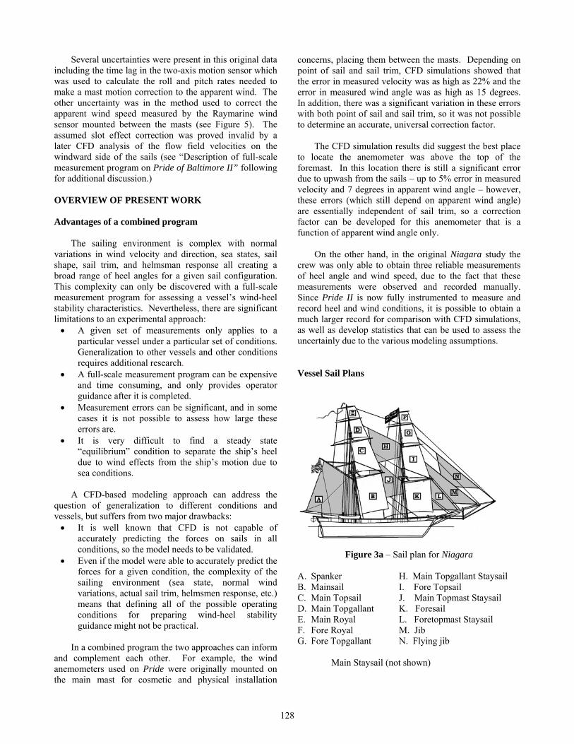
Figure 3a – Sail plan for Niagara

A. Spanker H. Main Topgallant Staysail B. Mainsail I. Fore Topsail C. Main Topsail J. Main Topmast Staysail D. Main Topgallant K. Foresail E. Main Royal L. Foretopmast Staysail F. Fore Royal M. Jib G. Fore Topgallant N. Flying jib

Main Staysail (not shown)

128

Figure 3b - Pride of Baltimore II. A key to sail

combination numbers for Pride II is found in Appendix A. Description of CFD-based modeling program

The present CFD-based model is a refinement of the

model described by Lasher et. al. (2007). This new CFD-based model (see Appendix B for computational details) was used for both vessels to calculate the heeling moment for a commonly used sail combination at apparent wind angles varying from close hauled to a beam reach. At each apparent wind angle the angles of attack of the sails were systematically varied to find two conditions – the sail angles that produced the maximum heeling moment, and the sail angles that produced the maximum driving force. This typically required about 20 separate simulations per apparent wind angle, which produced data that can be used to analyze the effects of sail interaction as a function of sail trim.

For Niagara, the sail combination consisted of both

topsails, the spanker with one reef, the jib, and the foretopmast staysail, and the minimum apparent wind angle was 50 degrees. Figure 4a shows the predicted steady-state heeling moment vs. apparent wind angle for Niagara. For Niagara, only the maximum heeling moment is shown as a sufficient number of simulations for maximum drive were not performed for all apparent wind angles. The maximum CFD-predicted heeling moment for Niagara occurs at an apparent wind angle of approximately 75 degrees.

Figure 4a – predicted heeling moment vs. apparent

wind angle for Niagara

For Pride II, the sail combination (defined as #13 in Miles et. al., 2007) consisting of the foresail, mainsail, square topsail with a single reef, fore staysail, jib, and jib topsail was used with a minimum apparent wind angle of 30 degrees. Figure 4b shows the resulting predicted steady-state heeling moment vs. apparent wind angle for Pride II (the differences in heeling moment between Niagara and Pride are due both to differences in the size of the ships, as well as different reference wind speeds used in the simulations). The maximum CFD-predicted heeling moment for Pride occurs at an apparent wind angle of approximately 60 degrees. The difference in apparent wind angle for maximum heeling moment is presumably due to differences in the design of the rigs (ie., predominantly square vs. fore-and-aft).

Figure 4b – CFD predicted heeling moment vs.

apparent wind angle for Pride II

When the wind is forward of the beam, the “maximum drive” case is more likely to occur than the “maximum heel” case on Pride II because it is presumed that the sails will be set to maximize performance due to relative ease of trimming her sails compared to the Niagara or when she is racing. Sail trim for maximum drive is less likely to occur on Niagara due to a number of factors including her size and the risks of backing the square sails; however, maximum drive is a clearly defined metric which can be optimized.

The maximum heeling moment condition can occur,

sometimes unexpectedly, for example, if either vessel is sailing upwind and for some reason has to turn quickly downwind (i.e. reduce square sails by getting wind behind them). Other causes for the maximum heeling moment condition are sails that are badly over-trimmed because of rig limitations, such as extreme mast rake and/or high vessel inertia and rig complexity, that cause slow responses by sail trimmers and/or helmsmen during lifts and heading gusts and during vessel maneuvers. This is less of a problem on modern racing sailboats where the helmsman and sail trimmers are able to more quickly adjust during apparent wind variations.

129

The heeling moment at maximum drive can be seen to “wiggle” in Figure 4b. This is due to the relative flatness of the drive force curve as a function of sail trim – that is, a small change in sail trim will produce a small change in driving force, but a more significant change in heeling moment. This distinction is important when racing, since the crew will accept high heel angles to maximize speed. However, there are many cases where accepting a slightly lower drive force in exchange for a more significant reduction in heeling moment is desirable. A more useful metric than maximum drive force would be maximum speed, but this can only be found by coupling the sail forces with a model for hull forces – something that is impractical with the current modeling process.

If the steady state model represented actual sailing

conditions, one would expect that the steady state heel angle seen by the ship would never exceed the predicted steady state “maximum heel” condition, and that it would generally be near the “maximum drive” condition, depending on how well the sails are trimmed. Since the sails can be completely luffed, the actual heel angle can be significantly less than either of these; however, no attempt has been made to model this condition.

An additional goal of the full-scale experimental

program (beyond validating the model) is to determine how likely the ship is to be operating at either of the nominal conditions (maximum heel or maximum drive) defined in the present analysis. For example, we hope to eventually be able make a statement such as “the actual heel angle was within 2 degrees of the predicted “maximum force” angle 50% of the time, and was within 2 degrees of the predicted “maximum heel” angle 5% of the time.”

Description of full-scale measurement program on Pride of Baltimore II

Shortly after the two groups started working together, the CFD model was used to calculate the sail forces for an initial set of sail and wind combinations on the Pride of Baltimore II. It was thought that the use of CFD to predict steady-state sail forces would greatly enhance the operator guidance goals, since only a more limited set of full-scale validation measurements would be needed to extend the SNAME SLIP (now SLEP) project (Miles et. al., 2007) to a variety of traditional sailing vessels.

This CFD analysis discovered that a five sail combination of 4 Lowers (4L) plus the Square Topsail (SQT) used by Pride II in many typical wind conditions act as a wind dam, slowing down the apparent wind and changing its apparent direction well to windward of the masts and beyond the location of the port and starboard Young Marine Jr. wind sensors added in 2007 (see Figure 5). This discovery invalidated the concept of measuring apparent wind 10 feet to windward and in the slot between

the masts, so the wing sensors were removed at the end of the 2007 season to be used on other traditional sailing vessels who will participate in this multi-year project.

Figure 5 – 2007 season wind sensor array on Pride II

This CFD analysis resulted in the decision to purchase

a Young Ultrasonic Anemometer to mount at the top of the foremast on Pride of Baltimore II, well above any of the normal sails. The anemometer is shown in Figure 6.

Figure 6 – Young Ultrasonic anemometer of the type

mounted on top of the fore-topmast of Pride II

Measurements from this system gave a number of data points to attempt to validate the steady-state CFD model of Pride II. This system was installed on Pride II along with John Womack’s new data acquisition package. Data taken during the Great Chesapeake Bay Schooner Race, October 10-14, 2007 showed very unsteady wind speed and heeling angles which when combined with non-quantifiable sensor lead/lag issues made the mast roll correction to the wind speed and direction essentially meaningless. We were also unable to log all the sensor data from Pride II because of incompatible data strings. 2008 Full Scale Data

It was then concluded that a fully integrated wind

sensor plus rate gyros and data acquisition package such as the B&G WTP2 system is needed (similar to that used aboard the Volvo 70 ocean racers and the America’s Cup class boats). The use of rate gyros is the only known method for correcting the wind sensor for mast motion and properly logging the data from a compatible set of sensors using the B&G Deckman software. The correction

130

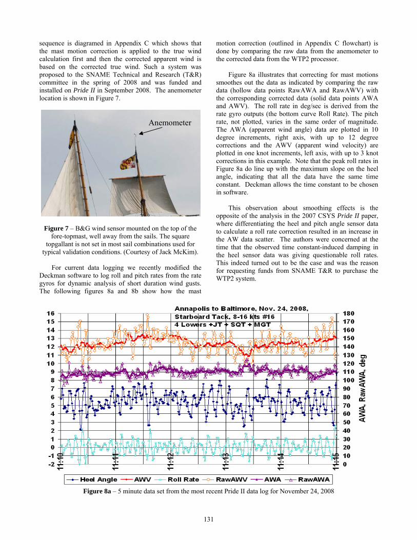
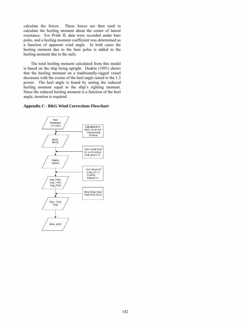
sequence is diagramed in Appendix C which shows that the mast motion correction is applied to the true wind calculation first and then the corrected apparent wind is based on the corrected true wind. Such a system was proposed to the SNAME Technical and Research (T&R) committee in the spring of 2008 and was funded and installed on Pride II in September 2008. The anemometer location is shown in Figure 7.

Figure 7 – B&G wind sensor mounted on the top of the fore-topmast, well away from the sails. The square

topgallant is not set in most sail combinations used for typical validation conditions. (Courtesy of Jack McKim).

For current data logging we recently modified the

Deckman software to log roll and pitch rates from the rate gyros for dynamic analysis of short duration wind gusts. The following figures 8a and 8b show how the mast

motion correction (outlined in Appendix C flowchart) is done by comparing the raw data from the anemometer to the corrected data from the WTP2 processor.

Figure 8a illustrates that correcting for mast motions

smoothes out the data as indicated by comparing the raw data (hollow data points RawAWA and RawAWV) with the corresponding corrected data (solid data points AWA and AWV). The roll rate in deg/sec is derived from the rate gyro outputs (the bottom curve Roll Rate). The pitch rate, not plotted, varies in the same order of magnitude. The AWA (apparent wind angle) data are plotted in 10 degree increments, right axis, with up to 12 degree corrections and the AWV (apparent wind velocity) are plotted in one knot increments, left axis, with up to 3 knot corrections in this example. Note that the peak roll rates in Figure 8a do line up with the maximum slope on the heel angle, indicating that all the data have the same time constant. Deckman allows the time constant to be chosen in software.

Anemometer

This observation about smoothing effects is the

opposite of the analysis in the 2007 CSYS Pride II paper, where differentiating the heel and pitch angle sensor data to calculate a roll rate correction resulted in an increase in the AW data scatter. The authors were concerned at the time that the observed time constant-induced damping in the heel sensor data was giving questionable roll rates. This indeed turned out to be the case and was the reason for requesting funds from SNAME T&R to purchase the WTP2 system.

Figure 8a – 5 minute data set from the most recent Pride II data log for November 24, 2008

131

Captain Miles installed the new B&G system when he

returned to Pride II, still on the Great Lakes in early September. The apparent wind angle calibration was done on September 14 after taking un-calibrated AWA data during the Prince Edward Island Race on September 13. Calibrated data were taken during the Halifax Race on September 17th, the New York City Races on October 2nd and 3rd, and a series of maneuvers just above the Bay Bridge on October 8th. Once back in Baltimore, Matt Fries of B&G wrote a software patch to record the output of the 3-axis gyro to obtain logs of the pitch, roll and yaw rates. This patch was used to obtain excellent data from the day-sail to Annapolis on November 19th, the day-sails on the 21st and 22nd and the day-sail back to Baltimore on November 24th. Much of the data used in this paper are from that last sailing day of the season for which the standard day-sail combination #16 was used. (See Appendix A for combination key)

From Figure 8b, note the difficulty in establishing

even quasi-static conditions. The wide swings in heel angle are associated with wind gusts (both speed and direction) that produce far-from-equilibrium conditions

which cannot be used as steady-state validation data. A useful parameter is to observe what happens to AWV2/HA, which should be a constant for the condition where wind heel moment equals the vessel’s righting moment, since the steady state heeling moment varies with the square of the apparent wind speed. This is confirmed in Figure 8b, where the hollow green data (AWV2/HA), is relatively consistent over a wide range of wind speeds and heel angles.

Also note that the AWV2/HA parameter drops

dramatically during increasing rolls and rises dramatically during roll back as illustrated in Figure 8c, an expansion of Figure 8b. Near time 11:10:20, a 6 degree lift drops the AWV by 0.5 knots and reduces the heel angle sharply which produces a peak in AWV2/HA. A sharp lift around 11:11:35 does the same to the heel angle with a change in AWV of only 0.22 knots.

Figure 8b – 2008 Data from B&G system. From the baseline y axis up: the aqua data (hollow squares) show the plus and minus variations in roll rate during the 30 minute time period. The green hollow data points show the square of the apparent wind velocity divided by the heel angle, a significant parameter. Dark blue diamonds represent heel angle, brown represents boat speed, purple triangles represent corrected apparent wind angle, red is corrected apparent wind speed, and orange is the true wind velocity. Note that bearing off just before 11:10 decreased the heel angle, but made only a small increase in average AWV2/HA even though both the true wind (top data set) and roll rate (lowest data set) increased.

132

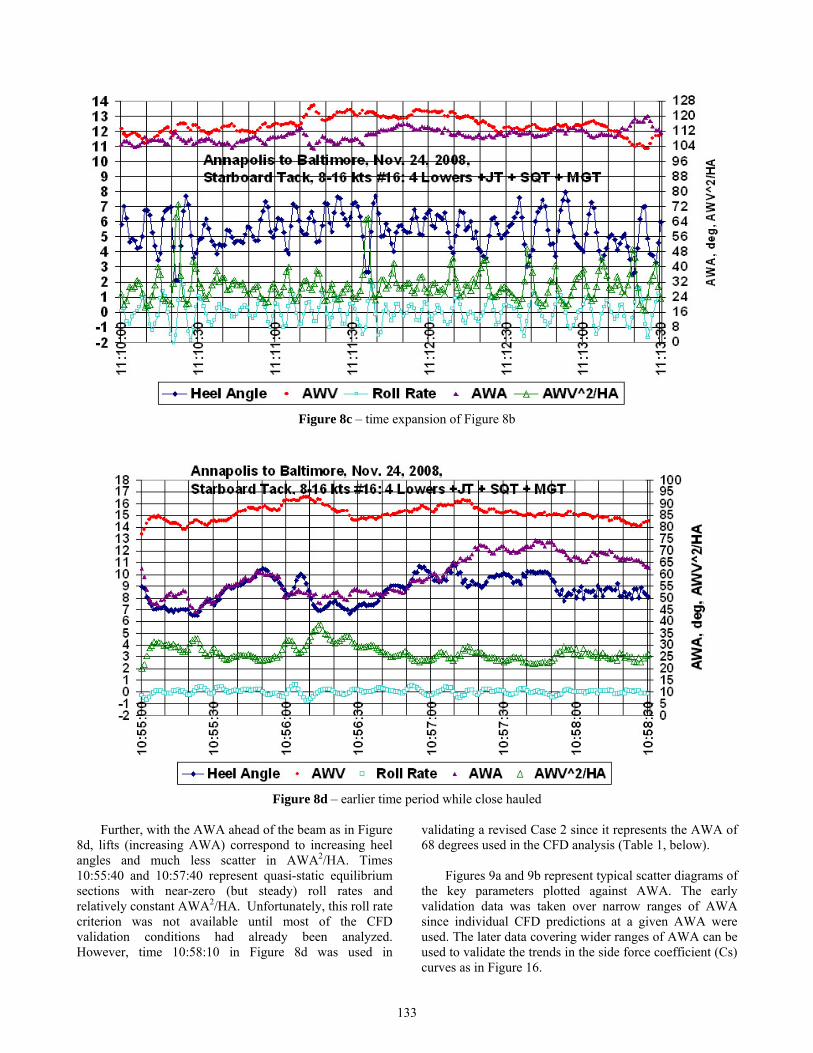
Figure 8c – time expansion of Figure 8b

Figure 8d – earlier time period while close hauled

Further, with the AWA ahead of the beam as in Figure

8d, lifts (increasing AWA) correspond to increasing heel angles and much less scatter in AWA2/HA. Times 10:55:40 and 10:57:40 represent quasi-static equilibrium sections with near-zero (but steady) roll rates and relatively constant AWA2/HA. Unfortunately, this roll rate criterion was not available until most of the CFD validation conditions had already been analyzed. However, time 10:58:10 in Figure 8d was used in

validating a revised Case 2 since it represents the AWA of 68 degrees used in the CFD analysis (Table 1, below).

Figures 9a and 9b represent typical scatter diagrams of

the key parameters plotted against AWA. The early validation data was taken over narrow ranges of AWA since individual CFD predictions at a given AWA were used. The later data covering wider ranges of AWA can be used to validate the trends in the side force coefficient (Cs) curves as in Figure 16.

133

Figure 9a – scatter diagram of primary parameters in Figure 8 above

Both TWA (True Wind Angle) and AWA values were

investigated for the x-axis but we settled on AWA since AWV2/HA, green circles, appears to vary around an apparent mean value except at very low apparent wind angles. For example in Figure 9a the mean value for AWV2/HA is about 24 to 26 over a range in AWA from 55 to 150 degrees. On the other hand, TWV2/HA varies from 4 to 16 over the same AWA range. Using true wind would require that the true wind speed must increase as the wind shifts aft to keep a steady heel angle.

Excellent full scale data for six different sail

combinations with reduced sail areas down to 22% of the standard four lowers plus three upper sails (#16) have been recorded. Data taken during a bear away experiment with all seven sails (#16) show interesting correlations at nearly

constant true wind speed (light blue) of apparent wind velocity (red) with resulting heel angle (dark blue) and the resulting square of AWV divided by heel angle (hollow green). This parameter should exhibit no scatter from steady state CFD calculations at a constant apparent wind angle (AWA). However in real sailing conditions, variations in both apparent wind speed (gusts) and direction (lifts and headers) create a useful scatter diagram for illustrating the effect of heading up and bearing away on heel angle. Heading up (decreasing AWA below 60 degrees) and bearing away (increasing AWA beyond 90 degrees) both serve to reduce heel angles. This is a well known fact but seldom quantified by a scatter diagrams, now possible with the new data acquisition system which corrects for mast motion.

Figure 9b – scatter diagram showing variations in a relatively constant true wind

134

Figure 10 – data from the New York City Race of October 2 in high, gusty winds using the reduced sail combination 19

Figure 10 shows the necessity of choosing a relatively constant AWV for steady-state validation efforts. The wide variations in AWV and HA as opposed to Figures 9a or 9b produce a variable value for AWV2/HA over the full range of AWA’s.

The September data used for validation purposes were

mostly taken at apparent wind angles much less than 90 degrees. However, the New York City Races on October 2 and 3 and a systematic series of tests in the mid-Chesapeake Bay on October 8th revealed that we needed to look more closely at the beam reaching condition, which appeared to have the greatest heel angles, especially when the crew cannot trim the sails easily to follow the effects of lifts and headers. Note this confirms the previously discussed CFD studies, (see Figure 4b,) showing the maximum heeling moment occurring at AWA’s greater than 60 to 80 degrees.

Using beam reaching conditions for validation

purposes also works to keep the AWV2/HA at a relatively constant value over a wide range of AWA values as was demonstrated in Figures 9a and 9b. In Figure 11, even though AWV and heel angle are relatively constant, AWV2/HA varies from about 64 to 48 over a relatively short AWA range of 44 to 60 degrees, making this a more sensitive area for assessing the accuracy of the CFD model.

Figure 11 – variation in AWV2/HA at low apparent wind

angles

135

Table 1 – Summary of six validation cases with data from full-scale measurements. A definition of the sail combinations is provided in Appendix A.

VALIDATION OF CFD MODEL WITH EXPERIMENTAL DATA

In addition to the original validation described in

Lasher et. al. (2007), the model was used to predict the heel angle for Pride II for the six different validation cases summarized in Table 1. For each of these cases the sails in the model were adjusted until the maximum driving force was found, since Pride was racing and the sails were most likely trimmed to produce maximum driving force. The observed and predicted values are compared in Figure 12.

The uncertainty estimates were made based on the

visual scatter about a median value of AWV2/HA vs. the apparent mean value at any given AWA. It is only meant to be an approximate calculation in the absence of sufficient data to calculate a meaningful standard deviation.

Figure 12 – predicted vs. observed heel angles for Pride II

The error bars on the observed heel angle show the

positive uncertainty from Table 1. (The equal negative uncertainty does not plot.) For 4 of the 6 cases the agreement between the model and the data is good. In cases 1 and 6 the model predictions are within the

uncertainties, and for cases 2 and 5 they are within 11% of the observed values.

Case 3 is the only case where the predicted value was

well outside the uncertainty band and also lower than the observed value. From a safety prediction viewpoint this is the most troubling case; in the other cases the errors are either relatively small or the prediction is conservative. Case 3 also had the highest apparent wind angle of the six cases, and it is hypothesized that the reason for the significant underprediction of the heel angle is that the sails may have been overtrimmed, as discussed earlier. If the worst case (i.e., maximum heeling moment) value from the CFD simulation is used rather than the maximum drive value, the predicted heel angle increases to 9.2 degrees, which is 18% higher than the observed heel angle. This shows that the observed angle is between the “maximum drive” and “maximum heel” values; however, further analysis of high apparent wind angle cases will be necessary to resolve this question, as discussed in more detail below.

For the fourth case the predicted heel angle is

significantly greater than the measured value (21% higher) and well outside the uncertainty band. This may be due in part to the fact that the square topsail had been braced back (i.e., the angle of attack was reduced) about 10-15 degrees to reduce the heeling moment in gusts, so the sails were not trimmed to produce maximum drive. An additional CFD analysis was performed with the square topsail set at an angle of attack 15 degrees less than that which produced the maximum driving force. The resulting predicted heel angle in this case was 15.4 degrees, which is within 2% of the measured value.

Since it is difficult to accurately record the actual sail

trim conditions, there is some uncertainty in the predictions. The previous analysis shows that the discrepancies can be explained by making reasonable assumptions about the sail trim. Other factors, such as lack of equilibrium as discussed earlier, could be

136

contributing to the difference between the predictions and experimental measurement. This shows that further analysis of the issues surrounding dynamic stability are necessary, and that the present validation results should be considered preliminary.

DEVELOPMENT OF A SIMPLIFIED MODEL FOR SAIL FORCES

While the CFD-based model described appears to be

reasonably accurate, it suffers from one major drawback – it takes approximately 5-6 hours of CPU time to perform a simulation for one case consisting of a single apparent wind angle and sail combination, with multiple sail angles of attack. It typically takes about 20 different cases to determine the sail trim that produces maximum heeling moment and the heeling moment at maximum drive for each apparent wind angle. The analysis of a single apparent wind angle is in excess of 100 hours; multiply this by the number of apparent wind angles and sail combinations of interest, and the required CPU time will be measured in years rather than hours. A more efficient method is clearly required.

A traditional approach is to identify an appropriate

side force coefficient and use it to calculate the heeling moment (Skene, 2001). Two questions must be addressed to determine if this approach is satisfactory:

1. Can the integration of stresses over the sail surfaces

be replaced with a single force applied at the sail centroid and get the same answer? In other words, does the force on a sail act reasonably close to the sail’s geometric centroid?

2. Can an appropriate side force coefficient be identified that will reasonably predict the heel angle under various conditions, or can a model for side force coefficients be developed that takes into account sail type, sail setting, and apparent wind angle?

To answer the first question, the upright heeling moment for Niagara was computed by multiplying the side force of each sail by the distance of the centroid of that sail from the center of lateral resistance. These results are plotted against the heeling moment calculated by direct integration of the stresses in Figure 13. The diagonal line shows what would be obtained if these two calculations of heeling moment were identical; the squares are the actual values. It can be seen from this figure that very little error is present in assuming that the sail forces act at the sail geometric centroids. One would assume that the center of pressure would be below the geometric centriod, since the water acts as a symmetry plane; however, the velocity increases as you get further from the water surface, and this has the effect of moving the center of pressure up. The two effects

essentially cancel each other, and the net force acts very close to the sail’s centriod.

Figure 13 – Niagara’s upright heeling moment calculated

by integration of stresses on sails (horizontal axis) and multiplying force on sail by distance of geometric centroid of sail to underwater center of lateral resistance (vertical axis). Distance from the diagonal line indicates error in

the calculation. To answer the second question, data from the previous

simulations were used to calculate the side force coefficient for Niagara’s foretopsail, as shown in Figure 14. One of the advantages of CFD is that it is possible to determine the forces on each sail independently while other sails are present – something that would be impossible on the ship and very difficult in a wind tunnel.

Figure 14 – side force coefficient vs. angle of attack

for Niagara’s foretopsail. The variation with apparent wind angle is due to the interaction of the foretopsail with

the other sails.

137

The side force coefficient is clearly a strong function of both angle of attack of the sail as well as apparent wind angle (due to interactions with the other sails). The coefficient is highest for sailing upwind thorough a beam reach (maximum side force occurs at 75 degrees AWA for Niagara as shown in Figure 4), and is minimal when the ship is on a broad reach or running. The maximum side force coefficient in this figure is approximately 1.7, and this is consistent across all of Niagara’s sails. A similar analysis was performed on the simulation results for Pride II, with comparable results. One could therefore use a value of 1.7 to find the “worst case”. The disadvantage of this approach is that it will not tell us anything about what the most likely heel angle will be; only how bad it can get.

An alternative approach to using a single side force

coefficient is to develop a side force coefficient model that is a function of sail type, apparent wind angle, and sail angle of attack. For example, using the “maximum drive” and “maximum heel” conditions described earlier, the side force coefficients for each sail on Pride II were determined from the CFD simulations, as shown in Figure 15:

Figure 15a – side force coefficient vs. apparent wind

angle for six sails on Pride II based on maximum drive case.

Figure 15b – side force coefficient vs. apparent wind angle for six sails on Pride II based on maximum heel

case.

It is clear from Figure 15 that the side force coefficient for a given sailing condition (i.e., maximum drive or maximum heel) is not a constant, but varies with each sail and apparent wind angle. For example, the jib topsail coefficient is among the highest at low apparent wind angles, but at high apparent wind angles, it must be eased to avoid blockage from the other headsails, so its side force coefficient is the lowest of the six sails. To determine how important these variations are, the heeling moment was calculated using the side force coefficients and compared to the integration results from the CFD simulation for three cases: using the actual Cs for each sail and apparent wind angle; using an average Cs of all six sails but varying with apparent wind angle; and using a single Cs that is the average for all sails and all apparent wind angles. In the first case (using the actual Cs for each sail) the error between the calculated heeling moment and that from integration was less than 3% for the maximum drive case and less than 4% for the maximum heel case, consistent with the results shown in Figure 13.

The average side force coefficients for all six sails as a

function of apparent wind angle are shown in Figure 16:

Figure 16 – average side force coefficient for Pride II at

each apparent wind angle

When these average values were used to calculate the heeling moment, the errors compared to the CFD integration results were less than 5% for the maximum drive case and less than 9% for the maximum heel case.

The overall average side force coefficients are 1.09 for

the maximum drive case and 1.38 for the maximum heel case. When these values were used, the errors in the computed heeling moments were as large as 22% and 42%, respectively. It is clear that the use of a single side force coefficient for all points of sail is not satisfactory, but the use of a force coefficient model such as the one shown in Figure 16 produces reasonable results. To determine whether additional corrections should be made to account for differences in sail type, the side force coefficients for Niagara using the maximum drive case were computed. The results are shown in Figure 17:

138

Figure 17a - Side force coefficients for Niagara at

maximum drive for individual sails,

Figure 17b– Side force coefficients for Niagara at

maximum drive for average for each apparent wind angle A comparison of Figure 17 with Figures 15 and 16 show similar trends with a few differences. The simulations for Pride II were limited to apparent wind angles of 90 degrees, whereas the Niagara simulations include broad reaching conditions. Under larger apparent wind angles it is possible to have very low or even negative heel angles since the topsails can be set at very low angles of attack (although this may not be practical since it induces roll and can be unsafe). The data taken from Pride II (see Figures 9a & 9b) do not show an increase in AWV2/HA at apparent wind angles greater than 90 degrees, which suggests that the sails may have been over trimmed. In particular, it may be that as the vessel falls off, the effective side force coefficient tends to increase from the maximum drive case towards the maximum heel case due to the difficulty of adjusting the fore and aft sails to wind shifts at these larger wind angles. Further simulations for Pride at larger angles are in progress to better assess this phenomena.

The 2007 Lasher paper demonstrated for NIAGARA that square sails braced to low angles of attack in a downwind situation can provide more driving force than if the square sails are trimmed to be square with the wind; i.e., in squared trim the square sails are stalled.

Aboard PRIDE there is the possible phenomenon of windward rolling when the square fore-topsail is braced to a low angle of attack to achieve maximum driving force while sailing downwind. This can, in the right sea conditions, generate synchronous rolling. So PRIDE almost never braces to low angle of attack. A similar phenomena was observed on Niagara when the square sails were braced to a low angle of attack. Separately, PRIDE’s fore and aft sails are often in an over trimmed state during wide sailing angle situations due to her raked masts and swept back shrouds that prevent the fore and aft sails from being trimmed to near 90 degrees of the ship. Usually PRIDE’s fore and aft sail trim is at the most 60-70 degrees as measured at the foot of the sail. Considering PRIDE’s fore and aft sails represent significantly more than 50% of the sail plan, perhaps the phenomenon referred to above is to be expected. Aboard NIAGARA, only 20% or less of her sail area is fore and aft and the huge proportion of sail that is square can be trimmed properly, even if by the lee, rather than in a stalled state of trim, when she is sailing downwind. The second difference is that the average side force coefficients for Niagara are about 11% less than the comparable coefficients for Pride (compare Figure 16 with Figure 17b). The force coefficients are also more uniform across sails for Niagara than they are for Pride at each apparent wind angle. This suggests that the side force coefficient model should include corrections at least for the rig type (i.e., square rig vs. fore and aft), if not for different combinations of sails. Future work is planned to better understand the differences in force coefficients with different rigs, and whether additional corrections could be built into the model to account for sail interaction effects.

It should be noted that the importance of this type of modeling is not limited to traditionally-rigged vessels. Commercial ships using sails to reduce fuel consumption will probably use rigs with several spars and sails due to the difficulty of handling large sails. For example, Fujiwara et. al (2005) report on the analysis of sail-sail and sail-hull interactions for a sail-assisted bulk carrier. They conclude that a better understanding of these interactions will be necessary if these types of ships are to be built, and models such as those being developed in the present work could be of value, at least during preliminary design stages.

CONCLUSIONS

While the CFD-based model has shown promise, there

are several issues that need to be addressed: 1. The current validation set is small and needs to be

expanded. Additional data need to be taken both on Pride II and on Niagara, and additional simulations need to be performed. Pride II is instrumented and

139

the processes for collecting the data are being refined; Niagara will receive similar instrumentation for the 2009 sailing season.

2. The question of under what conditions the vessel can

be assumed to be in static equilibrium needs to be clearly defined. Our preliminary analysis shows that a high correlation coefficient R2 of the parameter AWV2/HA indicates that the ship may be considered to be in quasi-static equilibrium, but a low R2 value does not necessarily indicate that the ship is not in quasi-static equilibrium. Additional metrics, including the evaluation of observed roll and pitch rates, need to be developed.

3. The difference between the apparent wind angle of

maximum heel from the CFD simulations compared to the experimental results needs to be understood. Specifically, the CFD results show that the maximum heeling moment should occur with the wind ahead of the beam, decreasing rapidly as the wind goes aft, whereas the experimental data show that the heeling moment remains relatively flat at apparent wind angles greater than 90 degrees. This may be due to over-trimming of the sails at higher apparent wind angles, and additional simulations are in progress to better understand the issue; however, it is an important question that must be resolved.

4. A more efficient model for calculating the sail forces

needs to be developed, as the CFD simulations are too time consuming for regular use. A possible approach for this model has been developed, and work is currently under way to assess its feasibility. Work is also underway to modify the spreadsheet used in the 2007 paper to include what has been learned from the CFD analysis, using the additional sail combinations and to account for an assumed boundary layer profile for the wind field.

ACKNOWLEDGMENTS

This work was supported by grants from the Behrend College Undergraduate Student Research Programs and generous instrumentation grants from the SNAME Technical and Research (T&R) Steering Committee. The support of Phil Mitchell and Matt Fries in setting up the B&G WTP2 system is greatly appreciated. REFERENCES Deakin, B., “Model Test Techniques Developed to Investigate the Wind Heeling Characteristics of Sailing Vessels and their Response to Gusts”, Proceedings of the Tenth Chesapeake Sailing Yacht Symposium, Annapolis, MD, February, 1991, pp. 83-93. Fluent 6.3 User’s Guide, Fluent, Inc., Lebanon, NH, 2006.

Fujiwawa, T. Hearn, G.E. Kitamura, F., Ueno, M. and Minami, Y. “Sail-Sail and Sail-Hull Interaction Effects of Hybrid-Sail Assisted Bulk Carrier”, Journal of Marine Science Technology, 2005, vol. 10, pp. 131-146. Harland, J. and Myers, M., Seamanship in the Age of Sail, Naval Institute Press, Annapolis, MD, 1984. Kerwin, J.E., “A Velocity Prediction Program for Ocean Racing Yachts”, Report no. 78-11, Massachusetts Institute of Technology, 1978. Lasher, W.C., Musho, T.D., McKee, K.C and Rybka, W., “An Aerodynamic Analysis of the U.S. Brig Niagara”, Proceedings of the Eighteenth Chesapeake Sailing Yacht Symposium, Annapolis, MD, March 2-3, 2007, pp. 185-197. Miles, J.C., Johnson, B., Womack, J. and Franzen, I, “SNAME’s Stability Letter Improvement Project (SLIP) for Passenger Sailing Vessels”, Proceedings of the Eighteenth Chesapeake Sailing Yacht Symposium, Annapolis, MD, March 2-3, 2007, pp. 165-184. Skene, N. L, Elements of Yacht Design, Sheridan House, Dobbs Ferry, NY, 2001, p. 92. APPENDIX Appendix A – Description of Niagara and Pride of Baltimore II

The U.S. Brig Niagara (Figure 1) is a re-construction of a sailing warship built for the Great Lakes portion of the War of 1812 between the U.S. and England. She has a dual mission of historic interpretation as well as skills preservation. Within this historic interpretation mission, the Niagara represents a warship from an important battle in the War of 1812, a story of naval history and seafaring as an industrial process. The other, and dominant, aspect of the mission is a skills preservation program carried out through the active sailing of the ship on 60 to 75 days each summer.

Niagara is also inspected by the U.S. Coast Guard (USCG) as a sailing school vessel (SSV) which falls under a different set of regulations than passenger vessels such as Pride of Baltimore II (described later). As a result, the crew is very concerned about wind-heel stability – that is, how much sail can she safely carry to maximize performance (crew/passenger enjoyment) and still have sufficient wind-heel stability margins to remain upright under various conditions.

Pride of Baltimore II, Figure 2, was commissioned in 1988 as a sailing memorial to her immediate predecessor, the original Pride of Baltimore, which was tragically sunk

140

by a sustained microburst off Puerto Rico in 1986, taking her captain and three crew members down with her. Pride I was built as a near exact reproduction (uninspected by the USCG, hence non-passenger carrying) of an 1812-era Chesapeake Bay topsail schooner privateer called Baltimore Clippers, which helped America win the Atlantic portion of the War of 1812. Pride II remains a faithful reproduction of a Chesapeake Bay Baltimore Clipper Privateer while also being a USCG inspected passenger-carrying traditional sailing vessel. Her mission is the representation of the origins of the American national anthem as a result of the contribution Baltimore Clippers made to the 1812 War as Baltimore-built privateers. She operates with a crew of 12, carrying general public passengers on both overnight voyages as well local day-sails.

The sail combination numbering system has been

changed from the 2007 paper as the projected standard 24 sail combinations were exceeded during the 2008 season for which data was obtained for sail combinations 16, 17, 18, 19, 20 and 22, giving a range of sail area ratios of 0.22 to 1.0 for the baseline combination #16.

Shorthand notation used to identify Pride II’s sails

Where M Main J Jib F Foresail S Fore Staysail 4L 4 Lowers = M+F+S+J JT Jib Topsail SQT Square Fore Topsail STG Square Top Gallant MGT Main Gaff Topsail

Appendix B - CFD Model Computational Details

Lasher et. al. (2007) presented the development of a CFD based model for predicting the forces and heeling moment on a square-rigged vessel due to the sails and

rigging. The sail forces were determined using Fluent (2006), a commercial Computational Fluid Dynamics (CFD) code. The forces on the spars and rigging were determined using a simple drag coefficient approach. An overview of the model will be presented here; readers interested in computational details can refer to the earlier paper.

The CFD simulations are used to find the forces on the

sails and the resulting heeling moment. Since Fluent (2006) is a Reynolds Averaged Navier Stokes Equation (RANS) code, the model accounts for both skin friction and separation effects. The heeling moment is calculated by integrating the moments due to pressures and shear stresses on the sails about the center of lateral resistance, which is assumed to be located at 40% of the ship’s draft below the waterline. The 40% value is based on the spanwise location of the center of pressure on an elliptically-loaded foil, and because this distance is small compared to the distance from the water to the sails, any error in this estimate will be negligible. Since the model is integrating the stresses, it does not assume that the aerodynamic forces are acting at the centroids of the sails.

The shapes of the sails are estimated based on

combination of photographic evidence and general knowledge of sail shape. Circular arcs are used for all sail cross-sections, which are a reasonable approximation for the types of sails used on traditionally-rigged vessels based on photographs from both Niagara and Pride II.

The inlet wind velocity is based on the atmospheric

boundary layer profile used in the IMS rule (Kerwin, 1978). The ship is stationary in the problem domain, so the reference wind is the apparent wind rather than the true wind. All computations are performed using a reference wind speed of 20 knots at a height of 10 meters above the water surface. Since the primary concern is in cases where the wind speed is high and the ship is sailing between a beam reach and upwind, the twist of the apparent wind is small and can be neglected.

When comparing the model to full-size data from the

ship, it is necessary to use the same wind velocity. Since the wind speed and direction at the anemometer are influenced by the sails, the CFD computations are used to determine what these would be at the anemometer location. These computed values are then used to scale the forces and moments from the simulation to the actual wind speeds on the ship, assuming that they vary by the square of the wind speed.

For Niagara, the heeling moment due to the spars and

rigging was calculated by assuming a drag coefficient of 1.13, which is what is used in the IMS rule (Kerwin, 1978). The spars and rigging are broken into segments based on their elevation from the water surface, and the velocity based on the boundary layer profile is used to

141

calculate the forces. These forces are then used to calculate the heeling moment about the center of lateral resistance. For Pride II, data were recorded under bare poles, and a heeling moment coefficient was determined as a function of apparent wind angle. In both cases the heeling moment due to the bare poles is added to the heeling moment due to the sails.

The total heeling moment calculated from this model

is based on the ship being upright. Deakin (1991) shows that the heeling moment on a traditionally-rigged vessel decreases with the cosine of the heel angle raised to the 1.3 power. The heel angle is found by setting the reduced heeling moment equal to the ship’s righting moment. Since the reduced heeling moment is a function of the heel angle, iteration is required. Appendix C - B&G Wind Corrections Flowchart

142