Pricing Options under Heston’s Stochastic

Volatility Model via Accelerated Explicit Finite

Differencing Methods

Conall O’Sullivan

University College Dublin∗

and

Stephen O’Sullivan

Dublin Institute of Technology

Current draft: June 2010.

Abstract

We present an acceleration technique, effective for explicit finite difference schemes

describing diffusive processes with nearly symmetric operators, called Super-Time-

Stepping (STS). The technique is applied to the two-factor problem of option pricing

under stochastic volatility. It is shown to significantly reduce the severity of the sta-

bility constraint known as the Courant-Friedrichs-Lewy condition whilst retaining the

simplicity of the chosen underlying explicit method.

For European and American put options under Heston’s stochastic volatility model

we demonstrate degrees of acceleration over standard explicit methods sufficient to

achieve comparable, or superior, efficiencies to a benchmark implicit scheme. We con-

clude that STS is a powerful tool for the numerical pricing of options and propose them

as the method-of-choice for exotic financial instruments in two and multi-factor models.

∗Address for correspondence: Conall O’Sullivan, Banking and Finance, The Michael Smurfit

Graduate School of Business, University College Dublin, Blackrock, Co. Dublin, Ireland. Email:

conall.osullivan@ucd.ie. The authors would like to thank the participants of the Bachelier World Congress

in Finance, London, July 2008 and the participants of the Quantitative Methods in Finance Conference,

Sydney, December 2009.

1 Introduction

The Black-Scholes partial differential equation (PDE), Black & Scholes (1973) and Merton

(1973), laid the foundations for modern derivatives pricing. However the assumptions

made in the Black-Scholes model are known to be overly restrictive. In particular, the

Black-Scholes model assumes that the underlying asset price follows a geometric Brownian

motion with a fixed volatility.

Many derivative pricing models have been developed subsequently which use more so-

phisticated stochastic processes for the underlying asset which result in a better match to

empirically observed details.

Using such stochastic processes is often more straightforward than relaxing the Black-

Scholes assumptions to allow for discrete time trading, transactions costs and other mar-

ket imperfections. Examples of more realistic stochastic processes include: jump-diffusion

(Merton, 1976); Levy (Cont & Tankov, 2004); stochastic volatility (SV) (Heston, 1993);

stochastic volatility jump-diffusion (Bates, 1996); and also combinations of these that ex-

hibit SV as well as jumps in both the asset price and volatility (Duffie et al., 2000).

In many of these cases there may be no analytical solution to the PDE describing the

corresponding vanilla European option price. The PDE describing the American analog

does not have a closed form solution in any of these models.

When a closed form solution does not exist one popular way to proceed is to solve

the PDE numerically using finite difference (FD) methods, see Wilmott et al. (1993) and

Tavella & Randall (2000).

Despite their increased complexity numerical valuations of options using FD methods

based on implicit discretizations are usually superior in terms of efficiency to approaches

based on conventional explicit discretizations. The principal reason for this is the Courant-

Friedrichs-Lewy (CFL) stability constraint on explicit schemes which limits the size of

the time step relative to the square of the spatial step size. In this paper, the restric-

tion that the CFL constraint imposes is reduced significantly using an acceleration tech-

nique for explicit algorithms known as Super-Time-Stepping (STS). STS was recently in-

troduced to the finance literature for the first time in the one-factor Black-Scholes setting

by O’Sullivan & O’Sullivan (2009) for vanilla European and American put options.

While the behaviour of STS has only been analytically established for symmetric opera-

tors Alexiades et al. (1996), O’Sullivan & O’Sullivan (2009) described the implementation

2

of a novel splitting approach to treating non-symmetric operators. This splitting method is

based on the unique decomposition of the operator into its symmetric and skew-symmetric

parts. The former may then be treated via STS while the latter is efficiently integrated

via a suitable scheme in a procedure introduced by O’Sullivan & Downes (2006, 2007). In

this way, O’Sullivan & O’Sullivan (2009) demonstrated formal stability for the accelerated

scheme and showed that the splitting procedure is unnecessary in the case of a weakly

non-symmetric operator.

In this work, we follow that precedent and do not split the operator. As will be shown,

for the problems under consideration here, the performance of STS does not appear to

suffer any discernable adverse implications to its stability properties as a result.

The contribution of this paper to computational finance is to extend the application

of the STS acceleration technology to the two-factor problem of pricing European and

American put options under Heston’s SV model. STS is compared to a number of standard

FD methods used frequently in the literature for SV options pricing. We demonstrate that

the efficiencies attained using the STS algorithm are comparable, and often superior, to

those of common implicit differencing techniques. Crucially, this acceleration is achieved

without any significant increase in implementation complexity relative to the underlying

standard explicit scheme.

There exist many methods to numerically solve European and American style options

using the PDE approach. Successive overrelaxation (SOR) is the most popular iterative

method for obtaining the solution in the European option case (see Crank (1984) for details)

while projected SOR (PSOR) (PSOR) (Cryer, 1971) is one of the most popular methods

used to solve higher dimensional linear complementarity problems (LCPs) that result from

pricing American options. With (P)SOR, as we refine the computational grid to obtain

more accurate option prices the number of iterations required to converge grows, however

this effect can be reduced by appropriate (problem dependent) tuning of the overrelaxation

parameter.

Other approaches used to numerically solve the option pricing PDE under the SV model

of Heston include: an ILU pre-conditioned conjugate gradient method with a penalty term

devised by Zvan et al. (1998) to handle the early exercise feature of American options; a

multigrid method used by Clarke & Parrot (1999) and Oosterlee (2003) to price American

options; a Hopscotch scheme applied by Kurpiel & Roncalli (2000) to price American op-

tions; a finite element approach constructed by Winkler et al. (2001) to price European and

3

barrier options.

A number of schemes used to solve LCPs were also compared by Ikonen & Toivanen

(2007a,b) including a PSOR method, a projected multigrid method, an operator splitting

method and a component wise splitting method. All of the schemes examined by these

authors displayed varying levels of superiority over the PSOR method in efficiently pricing

American options under the SV model.

All of the methods mentioned above, with the exception of the Hopscotch method which

is a mixed implicit-explicit method, are implicit algorithms which are faster but significantly

more complex in their implementation than their explicit differencing cousins. In particular,

these methods are global in the sense that the entire solution must be available in order to

advance any point and are therefore inherently difficult to parallelize.

The crucial difference in the STS algorithm allows explicit FD schemes to become viable

alternatives to their implicit counterparts. The relative simplicity of explicitly differenced

PDEs is inherited by the scheme including the local nature of the FD stencil. Parallelization

is therefore a trivial endeavor in this context.

This paper is arranged as follows.

Section II reviews Heston’s SV model, the corresponding PDEs describing vanilla Eu-

ropean and American option prices, and the associated boundary conditions. Section III

describes the implementation details required to construct the spatial (asset price and vari-

ance) grid and reviews the standard FD schemes used to benchmark the STS implementa-

tion employed. Section IV introduces the STS technique. The application of STS to option

pricing under SV is the main contribution of the paper. Section V contains comparative

timings and discussion of results. Finally, in Section VI, we offer concluding remarks.

2 Review

This section provides a review of the option pricing PDE and associated boundary condi-

tions for both European and American options under Heston’s SV model.

4

2.1 Heston’s Stochastic Volatility Model

Heston’s risk neutral SV model can be written as follows:

dxt = rxtdt +√

ytxtdzt,

dyt = {α (β − yt) − λγ√

yt}dt + γ√

ytdwt, (1)

ρdt = dztdwt,

where xt and yt are the asset price and variance at time t respectively, r is the risk-free

rate, α is the mean reversion of the variance, β is the long run mean of the variance, γ is

the volatility of the variance, ρ is the correlation of the asset price and the variance and λ

is the market price of risk. We denote by u(x, y, τ) an option price with a time-to-maturity

of τ = T − t where t is the observation time and T is the expiry.

2.2 European Put Options

European options satisfy the following PDE under these asset price dynamics:

Lu =∂u

∂τ+ Au = 0, (2)

where L is a generalised Black-Scholes type operator and A is its spatial component defined

by

Au = −1

2yx2uxx − ργyxuxy −

1

2γ2yxuyy − rxux − {α (β − y) − λγ

√y}uy + ru. (3)

The payoff, or initial condition, on a Eurpoean put option is

u(x, y, 0) = g(x, y) = max [E − x, 0] . (4)

European put options satisfy

u(0, y, τ) = e−rτg(0, y) (5)

on the boundary of x = 0.

The PDE on the boundary y = 0 reduces to

Lu =∂u

∂τ+ Au =

∂u

∂τ− rxux − αβuy + ru = 0. (6)

5

We use the following asymptotic boundary conditions at x = ∞ and y = ∞:

limx→∞

∂u(x, y, τ)

∂x= 0; (7)

limy→∞

∂u(x, y, τ)

∂y= 0. (8)

This is the equivalent system to that described by Clarke & Parrot (1999), Ikonen & Toivanen

(2007b), Oosterlee (2003) and Zvan et al. (1998).

2.3 American Put Options

American options may be excercised early thereby demanding the price u must at least be

as large as the early exercise value g. This leads to the early exercise constraint u(x, y, τ) ≥g(x, y).

In the continuation region where the contraint is inactive u satisfies the same PDE as

the European option i.e. Lu = 0 as given by Eq. 2.

Combining these relations we can write the American option pricing problem as a time

dependent LCP (for example see Ikonen & Toivanen (2007b))

Lu ≥ g, u ≥ g,

(Lu) (u − g) = 0,(9)

in a domain {(x, y, τ) |x ≥ 0, y ≥ 0, τ ∈ [0, T ]}.

Note that the payoff or initial condition of the American put option is the same as the

European option.

At x = 0, the pertinent boundary condition is

u(0, y, τ) = g(0, y). (10)

The linear complementarity conditions on the boundary y = 0 are

Lu = ∂u∂τ + Au = ∂u

∂τ − rxux − αβuy + ru ≥ g, u ≥ g,

(Lu) (u − g) = 0.(11)

The boundary conditions at x = ∞ and y = ∞ are the same as those for the European

put option as given by Eq. 7 and Eq. 8.

6

3 Implementation Details

In this section we provide the implementation details of the FD methods considered in this

work.

Following Ikonen & Toivanen (2007b), we use grid generating functions to increase com-

putational efficiency by decreasing the density of mesh points away from regions of interest.

We also employ upwinding when the PDE becomes convection dominated to avoid spuri-

ous oscillations in these regions as described by Ikonen & Toivanen (2007b). Unlike these

authors, however, we use a conventional nine point stencil as opposed to their seven point

prescription.

3.1 Spatial Discretization on Non-Uniform Grids

The FD discretizations are constructed on a non-uniform grid

(xi, yj , τk) ∈ {0 = x0, . . . , xm = X} × {0 = y0, . . . , yn = Y } × {0 = τ0, . . . , τl = T} . (12)

Standard FD methods are used to discretise the spatial operator A in Eq. 3. Centred

FD is used for the diffusion terms and, in most cases, for the convection terms. However,

at certain boundaries, and in areas where convection dominates over diffusion, upwinding

is beneficial and one-sided differences are used. More details on the discretization scheme

used at the boundaries and on the implementation of upwinding techniques are given in A

and B respectively.

We now present a nine point stencil with respect to a reference point (xi, yj).

The spatial intervals used in the discretization are then given as

hl = xi − xi−1, hr = xi+1 − xi, hd = yj − yj−1, and hu = yj+1 − yj . (13)

For clarity of notation from this point on we denote u (xi, yj) as ui,j .

The central FD schemes used for the diffusion components at the inner points of the

7

computional mesh (away from the boundaries) are

∂2u

∂x2≈ aD

l ui−1,j + aDui,j + aDr ui+1,j ,

∂2u

∂y2≈ bD

d ui,j−1 + bDui,j + bDu ui,j+1,

∂2u

∂x∂y≈ cD

ldui−1,j−1 + cDl ui−1,j + cD

luui−1,j+1 (14)

+ cDd ui,j−1 + cDui,j + cD

u ui,j+1

+ cDrdui+1,j−1 + cD

r ui+1,j + cDruui+1,j+1,

where

aDl =

2

hl (hl + hr), aD =

−2

hlhr, aD

r =2

hr (hl + hr),

bDd =

2

hd (hd + hu), bD =

−2

hdhu, bD

u =2

hu (hd + hu),

cDld = aC

l bCd , cD

l = aCl bC , cD

lu = aCl bC

u , (15)

cDd = aCbC

d , cD = aCbC , cDu = aCbC

u ,

cDrd = aC

r bCd , cD

r = aCr bC , cD

ru = aCr bC

u .

The FD schemes used for the convection components at any inner points of the com-

putional mesh where upwinding is not necessary are

∂u

∂x≈ aC

l ui−1,j + aCui,j + aCr ui+1,j ,

∂u

∂y≈ bC

d ui,j−1 + bCui,j + bCu ui,j+1, (16)

where

aCl =

−hr

hl (hl + hr), aC =

hr − hl

hlhr, aC

r =hl

hr (hl + hr),

bCd =

−hu

hd (hd + hu), bC =

hu − hd

hdhu, bC

u =hd

hu (hd + hu). (17)

Substituting these approximations into Heston’s PDE for European options, Eq. 2, we

8

have

∂u

∂τ−

(

1

2yx2aD + ργyxcD +

1

2γ2bD + rxaC + α (β − y) bC

)

ui,j

−(

1

2yx2aD

l + ργyxcDl + rxaC

l

)

ui−1,j

−(

1

2yx2aD

r + ργyxcDr + rxaC

r

)

ui+1,j

−(

ργyxcDd +

1

2γ2bD

d + +α (β − y) bCd

)

ui,j−1 (18)

−(

ργyxcDu +

1

2γ2bD

u + +α (β − y) bCu

)

ui,j+1

−(

ργyxcDld

)

ui−1,j−1 −(

ργyxcDlu

)

ui−1,j+1

−(

ργyxcDrd

)

ui+1,j−1 −(

ργyxcDru

)

ui+1,j+1 = 0.

The governing PDE may then written compactly as

Lu =∂u

∂τ+ Au = 0, (19)

in which A is a nine component operator matrix given by

A =

Alu Au Aru

Al Ac Ar

Ald Ad Ard

, (20)

with

Ac = −(

1

2yx2aD + ργxycD +

1

2γ2ybD + rxaC + α (β − y) bC − r

)

,

Al = −(

1

2yx2aD

l + ργxycDl + rxaC

l

)

,

Ar = −(

1

2yx2aD

r + ργxycDr + rxaC

r

)

,

Ad = −(

1

2γ2ybD

d + ργxycDd + α (β − y) bC

d

)

, (21)

Au = −(

1

2γ2ybD

u + ργxycDu + α (β − y) bC

u

)

,

Ald = −ργxycDld, Alu = −ργxycD

lu

Ard = −ργxycDrd, Aru = −ργxycD

ru.

9

We have relegated discussion of the discretization techniques employed at the boundaries

to A, and on the interior in zones where upwinding is necessitated by the dominance of

convection effects in the solution to B.

The approach described above is easily applied to the case of American options as given

by the time dependent LCP Eq. 9.

3.2 Grid Generating Functions

Grid generating functions are used to increase the density of the computational nodes

around regions of importance in order to increase the efficiency of the method i.e. to reach

a desired accuracy level with less grid points. The grid in the x−direction is constructed

according to

xi+1 = xi + hr(xi) for i = 0, . . . , m, (22)

with the functional form used for the grid generating function in the x−direction, hr(xi),

given by:

hr(xi) = E +c

psinh

(

pxi + arcsinh(

−p

cE

))

for i = 0, . . . , m. (23)

as described by Kluge (2002).

This grid generating function increases the number of nodes around the exercise price E.

The parameter c controls the density of the grid points close to E relative to the density of

the grid points at xmax. The parameter p is obtained by requiring x0 +∑m

i=1 hr(xi) = xmax

and solving numerically for p.

By way of illustration, Figure 1(a) depicts the non-uniform grid step size versus the

stock price for x0 = 0, xmax = 20, m = 128, p = 0.2177 and c = 0.5. These parameters

result in a ratio of step sizes in the x-direction at xmax and E of 4.3939.

In the y−direction a linear grid generating function, hu(yj), is used where

yj+1 = yj + hu(yj) for j = 0, . . . , n. (24)

The grid generating function hu(yj) increases the density of grid points at low variance

values relative to high variance values and is specified by

hu(yj) =qj/n − 1

q − 1yj for j = 0, . . . , n. (25)

10

The parameter q is chosen to ensure that a given reference value in variance occurs

on some point on the grid, yk. For the tests under consideration in this work we choose

yk = 0.0625 or yk = 0.25.

Figure 1(b) plots the non-uniform grid step size against the variance y for yk = 0.0625, n =

64 and q = 4.0734. In this illustrative case, the ratio of step sizes in the y-direction at ymax

and yk is 2.1566.

3.3 Time Discretization

In this section the explict, implicit and Crank-Nicolson (CN) time discretization methods

are briefly described.

The Heston PDE for European options over the entire solution space can be written as

∂u

∂τ+ Au = 0, (26)

where A is a block tridiagonal (m+1)(n+1)×(m+1)(n+1) matrix, u is a vector of length

(m+1)(n+1), m is the number of steps in the x−direction and n is the number of steps in

the y−direction. The vector u and tridiagonal matrix A are constructed by stacking each

solution uij and corresponding nine component operator matrix A into a column vector

and block tridiagonal matrix respectively, for i = 0, . . . , m and j = 0, . . . , n.

We begin by introducing the θ-method of discretization. Applied to Eq. 26 we obtain

u(k+1) − u(k)

∆τ+ θAu(k+1) + (1 − θ)Au(k) = 0

⇒ (I + θ∆τA)u(k+1) − (I − (1 − θ)∆τA)u(k) = 0, for k = 0, 1, . . . , l − 1.

This can be written more compactly as

Bu(k+1) − Cu(k) = 0, (27)

where B = I + θ∆τA and C = I − (1 − θ)∆τA.

For American options the scheme in Eq. 27 becomes a time dependent LCP as described

in Eq. 9

Bu(k+1) ≥ Cu(k), u(k+1) ≥ g(

Bu(k+1) − Cu(k))T (

u(k+1) − g)

= 0,(28)

11

where g is the early exercise value of the option.

When θ = 0 the θ-method corresponds to the explicit Euler scheme. This scheme

is first order accurate in time and second order accurate in space. The Euler scheme is

very simple to implement, however, stability depends on the size of the time step which

is in turn dictated by the spatial step size and the coefficients of the governing PDE (see

Wilmott et al. (1993); Tavella & Randall (2000) for further details). In particular when

correlation ρ = 0, the theoretical upper limit on the time step is given by

∆τexpl ≤ min0≤i≤m

0≤j≤n

[

x2i yj

h (xi)2 +

γ2yj

h (yj)2

]−1

. (29)

In the more general case of non-zero correlation Eq. 29 is found to be an effective estimate

of the critical upper limit on the time step in the test cases considered in this paper.

This constraint on the time step is known as the Courant-Friedrichs-Lewy (CFL) stability

constraint and can be severely restrictive.

When θ = 1 the θ-method corresponds to the fully implicit scheme. The fully implicit

scheme is first order accurate in time, second order accurate in space and has no limitations

on the size of the time-step for stability, however, the desired accuracy of the solution still

imposes a constraint on the minimum number of time steps that may be used.

An alternative approach frequently used in the literature is the CN scheme which cor-

responds to θ = 1/2. The CN scheme is second order accurate in time and space. Similarly

to the fully implicit method, CN has no limitations on the size of the time-step for stability.

However the CN method can lead to solutions with spurious oscillations if the initial value

is not smooth (which is the case for option payoffs). To alleviate this problem Rannacher

(1984) time-stepping is typically used in the CN algorthim1.

In the fully implicit and CN schemes, LCPs can be solved iteratively at each time

step by employing any of a number of methods including PSOR, projected multigrid,

and the penalty method (see Clarke & Parrot (1999); Oosterlee (2003); Ikonen & Toivanen

(2007b)). Direct methods also exist such as the formulation presented by Ikonen & Toivanen

(2007b) of the Brennan & Schwartz (1977) UL decomposition algorithm.

1Rannacher time-stepping is where the first few time steps are performed with the fully implicit scheme

with a time step size of ∆τ/2 and thereafter the time steps are performed with the CN scheme with a time

step size of ∆τ . We use the first four steps with the implicit scheme and the remaining l − 4 steps with the

CN scheme.

12

We elect CN with PSOR, denoted CN-PSOR, as the standard benchmark scheme for

comparison with the proposed STS approach in tests solving Eq. 28. CN-PSOR is a suitable

choice due to its competitive performance with respect to other methods and its widespread

usage (e.g. Tavella & Randall (2000); Wilmott et al. (1993)). A short description of the

PSOR algorithm is included in C for the reader’s reference.

The equation for the European option price, Eq. 2, may be solved analytically (Heston,

1993). However, as analytical solutions do not exist in general for exotic options with

European payoff functions, we test the efficacy of STS with respect to CN-SOR, a CN

scheme iteratively solved via simple successive overrelaxation (SOR).

Finally, the standard explicit scheme to first order accurate in time, denoted EXPL-1,

is included in the tests to assess the relative acceleration achieved by STS over its base

scheme in both the American and European cases.

4 Super-Time-Stepping

In the previous section we reviewed a number of well known time discretization approaches

frequently used in FD methods for the integration of time-dependent PDEs. This section

introduces an alternative time discretization method known as super-time-stepping (STS)

which can be used to accelerate conventional explicit schemes for parabolic problems with

nearly symmetric positive definite evolution operators.

In the following, we shall use the description of Alexiades et al. (1996), itself a variant of

a method presented by Gentzsch (1979), which is in turn essentially a pared-down Runge-

Kutta-Chebyshev (RKC) method (van der Houwen (1977); van der Houwen et al. (1980);

Verwer et al. (1990); Verwer (1996); Sommeijer et al. (1997)).

Despite the fact that the STS method is approximately 30 years old, it has been reported

in use by relatively few researchers. The instances in the literature of STS being used which

we are aware of are in engineering and physical disciplines. These include: nonlinear de-

generate convection-diffusion Evje et al. (2001); electromagnetic wave scattering Shi et al.

(2006); isotropic and anisotropic diffusion on biological membranes Sbalzarini et al. (2006);

and magnetic field diffusion in astrophysics O’Sullivan & Downes (2007); Mignone et al.

(2007). Recently, STS has been applied in finance and rigorously tested for the Black-

Scholes pricing model by O’Sullivan & O’Sullivan (2009) where it was shown to be compa-

rable, and in many cases superior, to the CN-SOR/CN-PSOR scheme in terms of accuracy

13

and computional speed for European/American put options.

To proceed we consider the PDE

∂u

∂τ+ Au = 0; u (0) = u0, (30)

and we assume a linear explicit scheme on u ∈ R(m+1)(n+1) of the form

uk+1 = (I − ∆τstsA)uk (31)

where the solutions at time levels k and k +1 are known and unknown respectively, I is the

identity matrix and A ∈ R(m+1)(n+1) ×R

(m+1)(n+1) is a symmetric positive definite matrix.

Eq. 31 corresponds to the θ = 0 instance of the θ-method corresponding to the explicit

Euler scheme as described in Section 3.3. For stability the CFL contraint requires that

|1 − ∆τλ| < 1 (32)

for all eigenvectors λ of A. The maximal value of ∆τ may therefore be defined by

∆τexpl ≡2

λmax(33)

where λmax is the largest eigenvalue of A.

The essence of STS is that rather than requiring stability at each step of the time

integration, Nsts sub-steps of varying size ∆τj (j = 1 to Nsts) are rolled together into a

single super-step ∆τsts according to

∆τsts =

Nsts∑

j=1

∆τj . (34)

and stability is only demanded at the end of the super-step 2. We write the compound

scheme as

uk+1 =

Nsts∏

j=1

(I − ∆τjA)

uk (35)

2Verwer (1996) has claimed that factorized RKC methods are impractical as they suffer from internal

instability. O’Sullivan & O’Sullivan (2009) find no evidence of any such instability influencing their solutions

for cases with Nsts<∼ 30.

14

and for stability we require

∣

∣

∣

∣

∣

∣

Nsts∏

j=1

(1 − ∆τjλ)

∣

∣

∣

∣

∣

∣

< 1 (36)

for all eigenvectors λ of A.

The properties of Chebyshev polynomials of degree Nsts (Markoff, 1916) provide the

means to explicitly enforce stability while maximizing ∆τsts. The optimal values for the

sub-steps obtained in this way are given by

∆τj = ∆τexpl

[

(−1 + ν) cos

(

2j − 1

Nsts

π

2

)

+ 1 + ν

]−1

(37)

where ν is a user defined damping factor. The scheme is stable for ν > 0 and unstable in

the limit ν → 0 with the property

∆τsts → N2sts∆τexpl as ν → 0. (38)

In practice the scheme may be marginally stable for low enough values of ν for a given

choice of Nsts. A balance between robustness and acceleration should therefore be struck

by the user with appropriate choices of the two free parameters.

We illustrate the efficacy of the acceleration process for Nsts = 30 in Figure 2 for various

choices of ν. It can be seen that the first substep may be up to 25 times the stable limit

for a standard explicit integration as ν → 0 but subsequent substeps become small. The

effect of this is a cumulative error cancellation which recovers stability over the composite

superstep. Crucially, there is a net payoff in terms of the size of the superstep with respect

to Nsts steps of size ∆texpl according to equation 38.

STS applied directly as described above results in a scheme which is first order in

time (Alexiades et al., 1996). From this point we shall refer to this scheme as the STS-1

scheme. It is not possible to introduce additional temporal structure to an STS step since

intermediate values obtained during an STS cycle are physically meaningless and may not

be used as approximations to the solution in any sense. Therefore, predictor-corrector style

methods are not applicable should higher order convergence be required. On the other

hand, we have found that Richardson extrapolation (RE) works well. By this method

15

all the advantages of the STS-1 method are easily transferred to second (or higher) order

schemes.

The principal advantage of the STS method is not efficiency however, but simplicity.

Explicit discretizations of even the most complex systems of parabolic equations are very

straightforward within this discretization paradigm. In particular, implementation of adap-

tive mesh refinement (AMR) technologies and/or parallelization via domain decomposition

techniques present no great challenges from within an explicit framework. On the con-

trary, when implicit methods are involved, tackling problems of even a moderate level of

complexity can be an exceedingly intricate task, especially in parallel applications.

Note that although formal results only exist for linear schemes, there is ample evidence,

as described above, that non-linear target systems may be equally amenable to the STS

method. Formally, stability of the STS scheme is assured if A in equation (35) is symmetric

positive definite, Alexiades et al. (1996). However, in the Black Scholes PDE and the more

general Heston PDE the spatial operator A is weakly non-symmetric.

In the Black Scholes case a formal stability analysis for an alternative discretization of

the non-symmetric Black Scholes spatial operator A is given in O’Sullivan & O’Sullivan

(2009). The scheme presented therein is formally stable under application of STS to the

symmetric component of the multiplicitavely split operator. The skew symmetric part

of the operator is then integrated via a novel scheme developed by O’Sullivan & Downes

(2006, 2007). While the split scheme presented by O’Sullivan & O’Sullivan (2009) is for-

mally stable and may be of particular interest for systems with moderate to strong skew

symmetric evolution operators, it was found by these authors that this alternative scheme

was not strictly necessary for weakly non-symmetric operators. In agreement with this

result, we find that splitting is unnecessary and that direct application of the STS scheme

to the Heston PDE is appropriate even though the Heston spatial operator A is not fully

symmetric.

Before comparing the performance of the STS method applied via equation (35) to the

FD schemes described in Section 3.3 we include a brief section on the use of RE in the STS

scheme.

16

4.1 Richardson Extrapolation

In this paper we employ two RE methods to render STS schemes second order accurate in

time.

The first approach is to use RE in a step-wise fashion. We assume a smoothly convergent

first order accurate method for the temporal integration of the semi-discrete equation (30)

with exact solution u∆x,∆y(x, y, τ) on a grid with spatial intervals ∆x, ∆y. Given a second

order accurate solution at time level k such that uki,j = u∆x,∆y(i∆x, j∆y, k∆τ) + (L −

k)O(∆τ3) we may take a single step of size ∆τ to approximate the solution at time level

k+1 using uk+1ij (∆τ) = u∆x,∆y(i∆x, j∆y, (k+1)∆τ)+C∆τ2+O(∆τ3) for some constant C

determined by the leading truncation error term of the scheme. Similarly, taking two steps

of size ∆τ/2, we have uk+1ij (∆τ/2) = u∆x,∆y(i∆x, j∆y, (k + 1)∆τ) + (C/2)∆τ2 +O(∆τ3).

Subtracting the expression for uk+1ij (∆τ) from twice the expression for uk+1

ij (∆τ/2) yields

a second order advancement in the solution from time level k to level k + 1 according to

uk+1ij = 2uk+1

ij (∆τ/2) − uk+1ij (∆τ), for k = 0, 1, . . . , l − 1. (39)

We also consider the more usual post-processed form which requires two independently

derived solutions for use in the extrapolation of the final solution ulij = 2ul

ij(∆τ/2) −ul

ij(∆τ), see for example Geske & Johnson (1984).

We refer to the former approach as local RE and the latter as global RE. The significant

difference is that, for local RE, a second order solution is immediately available at every

temporal mesh point. For global RE, this would require significant additional data storage

and handling. However, we find that global RE is less prone to numerical oscillations for

very small values of the damping parameter ν and is therefore preferable in general for use

with STS.

We note that RE is computationally more expensive than some other higher order

reconstructions. It requires 50% more computational effort than the predictor-corrector

approach on a per-step basis. However, it is simple to implement as it merely requires a

reapplication of the first order scheme. When used with STS it is of greater applicability

than CN-PSOR as shall be demonstrated.

17

5 Numerical Experiments

In this section we analyse the efficiency of the STS accelerated explicit scheme relative to

the unaccelerated explicit scheme and a CN scheme applied to the pricing of European and

American options under Heston’s SV model.

The default parameters of the problem are chosen to be

E = 10, T = 0.25, r = 0.1, α = 5, β = 0.16, γ = 0.9, λ = 0, and ρ = 0.1,

in order to permit direct comparison with the results of Zvan et al. (1998); Clarke & Parrot

(1999); Oosterlee (2003); Ikonen & Toivanen (2007b)3. The computational domain’s extent

is defined by setting xmin = 0, xmax = 20 and ymin = 0, ymax = 1. These values are again

chosen for consistency with the referenced works. We note, however, that xmax = 20 is

close enough to the exercise price E = 10 for the influence of the boundary to be apparent

on the solution. This point is discussed further in the subsequent error analysis of this

section. Grid generating functions, as described in section 3.2, are used to prescribe the

interior grid points. The convention we use for a given test case for denoting the number

of stock price steps, variance steps and time steps respectively is {m, n, l}.

Firstly, by way of an illustration the behaviour of STS driven acceleration as ν → 0 over

the time-to-maturity of the option T , we fix Nsts = 30 and consider the performance of

STS-1 for various small values of ν. Panel (a) of Figure 3 shows the number of supersteps,

l, required to complete the integration over time T versus the damping parameter ν on

a grid where (m, n) = (512, 256), the finest grid test case considered in the experiments

below. The convergence of l to 77 as ν → 0 is clearly evident in panel (b) (where the

abcissa are logarithmic rather than linear in ν). From Eq. 38, and using the minimum

number of explicit steps required for stability on this grid (estimated to be lexpl = 68, 878

from Eq. 29), we expect a limiting value of l ≈ 77. This is clearly in good agreement with

our experimentally derived value and repesents a speed-up by a factor of approximately 30

relative to the explicit method.

We note that accelerated schemes are not stable for vanishing ν and some small but

finite value of ν is required. By way of illustration of this detail, Figure 3 includes a reference

line at l = 81 corresponding to the acceleration obtained for ν = 4 × 10−5. This is the

3Other parameter settings were chosen including cases in which the Feller condition was not satisfied.

However results were broadly similar across all parameter settings examined.

18

experimentally derived stability limit for the STS-1 scheme below which prices are found

to exhibit spurious oscillations. At this value of ν a speed-up factor of approximately 28 is

achieved.

Stable solutions are guaranteed on all the grid resolutions in the experiments considered

below for ν = 0.0006. Moreover, as the grid resolution is increased the damping parameter

can be pushed closer to zero whilst still maintaining stable solutions.

In the following sections we shall examine the behaviour of the schemes as both the

spatial and temporal resolutions are increased simulataneously. For EXPL-1, in order to

achieve a stable solution the number of timesteps is increased by 4 for every doubling of

the spatial resolution. In all other cases the resolution in time is scaled linearly with the

spatial resolution.

5.1 European Options

We now present a series of test results for the pricing of European put options under

Heston’s SV model.

Table 1 displays European put option prices at five stock prices x = 8, . . . , 12 for an

initial variance y = 0.0625 at a number of different resolutions. Five numerical schemes

are tabulated: the STS-1 method; the STS method with local RE (STS-RE-L); the STS

method with global RE (STS-RE-G); the standard explicit approach to first order accuracy

in time (EXPL-1); and the CN-SOR scheme. We will refer to the STS-RE-L and STS-RE-G

schemes collectively as the STS-2 schemes. Two reference methods derived via the semi-

analytical results obtained using the FFT approach of Carr & Madan (1999)4 and a high

resolution CN-SOR method are included for reference.

The CN-SOR European put prices are computed with a convergence tolerence measure

tol = 1 × 10−4 defined similarly to tol in C (tol = 1 × 10−5 on the high resolution grid).

These values are approximately optimal in the sense that we find decreasing the tolerance

increases the run time for the scheme without improving the accuracy. The overrelaxation

parameter is varied with the grid resolution to ensure optimal convergence rates for the

scheme. All European STS prices are computed with a fixed number of substeps Nsts = 30

and a fixed damping parameter of ν = 0.0006. The number of supersteps, l, is scaled in

4The accuracy of the FFT prices were ensured by varying the FFT inputs until the relative price changes

were of the order of 1 × 10−10.

19

proportion to the number of points on the spatial grid in each dimension.

It is clear from Table 1 that all five FD methods result in European put prices that

converge as expected to the reference prices as the grid and temporal resolutions increase.

To evaluate the rate of this convergence we examine the errors in the solutions obtained

from the FD schemes relative to reference prices.

Figure 4 illustrates the errors in the solutions obtained from the FD schemes as a

function of the stock price at an initial variance y = 0.0625 on a range of resolutions. As

stated previously, the boundary at xmax = 20 is close enough to the exercise price E = 10,

that the influence of the boundary conditions are evident in the solution. While we have

carried out tests with xmax moved to larger values and confirmed that boundary induced

errors may be reduced, as previously remarked, we use xmax = 20 for consistency with

the referenced tests from the literature. For the error analysis we use a high resolution

reference solution obtained via CN-SOR with (m, n, l) = (2048, 1024, 2050). Note that the

semi-analytical FFT results are inappropriate as the reference solution for this analysis

since they are not subject to the boundary conditions prescribed for the FD numerical

schemes. We note however that we have confirmed the high resolution CN-SOR solution

converges to the semi-analytical FFT solution at a rate of second order accuracy at ten

sample interior points (x, y) = ([8, 9, . . . , 12] × [0.0625, 0.25]).

The error in the prices is in good agreement in all cases. STS-1 demonstrates larger

errors than the others due to its lower (first) order of accuracy in time. Despite also

being first order in time, the error in the EXPL-1 solution is close to those of the second

order integrations. This is due to the substantially larger number of timesteps required

to maintain a stable solution which results in a negligible first order temporal error with

respect to the second order spatial error. The total error therefore takes on the second order

charasteristics of the spatial error. We also note that the plots are qualitively similar for

different variance values y, however, the errors do increase in magnitude across all schemes

when y is near the boundary values of y0 = 0 and yn = 1.

Table 2 displays the l2 norm errors calculated using ten European put prices at five

stock prices about the exercise price E, x = 8, 9, . . . , 12, and two different initial variance

values y = 0.0625 and y = 0.25. As before, since it is a first order accurate method in

time, the STS-1 method displays the largest errors in the l2 norm. We also found that the

explicit method displays the smallest l2 norm error values since, as previously remarked,

very high temporal resolution is necessary to maintain stability. We may also observe that

20

the STS-2 schemes provide l2 norm errors that are similar to standard explicit case. We

may deduce therefore that the temporal error in the STS-2 schemes is also small despite

the more efficient time integration. Finally, we note that, while not dramatically different,

the CN-SOR scheme has the highest l2 norm error of the second order schemes.

Table 2 also provides error ratios between test cases with successively increased reso-

lution. The error ratios for STS-1 are approximately 2 which is a consequence of scheme

with dominant first order temporal error. In the case of EXPL-1 the error ratios scale as

roughly 4 on doubling the spatial resolution. As remarked earlier, the temporal resolution

is necessarily very high for reasons of stability resulting in a negligible temporal error and

dominant second order spatial error. This is compatible with our assumption of a scheme

which is second order in space and first order in time. The remaining schemes yield ratios

of approximately 4 suggesting schemes which are second order both in space and time.

We remark that the convergence rates of the STS-2 methods are almost identical to the

CN-SOR and the standard explicit method.

Lastly, we note that table 2 gives CPU times for each test. These indicate that on the

finest grid the STS-1 method is least computationally expensive, followed by STS-RE-L,

STS-RE-G, CN-SOR and finally EXPL-1 in that order. Notably, the STS-2 methods are

approximately twice as efficient as the CN-SOR scheme. This is despite the advantage of

the overrelaxation parameter in CN-SOR being chosen experimentally to ensure the fastest

possible convergence of the algorithm in each case.

5.2 American Options

When pricing American options with the STS schemes, the early exercise constraint is

applied at the end of each superstep since the solution conditions inside the superstep are

not meaningful as option prices. Consequently, an increase (decrease) in the number of

supersteps results in an increase (decrease) in the frequency at which the early exercise

condition is enforced. This generates a trade-off in the speed of the algorithm versus the

resolution of the early exercise boundary. A similar trade-off in speed versus accuracy

typically arises for implicit methods. For PSOR, for example, projection (replacement of

the continuation value of the American option with its early exercise value when optimal)

must be carried out within each iteration (see C). A direct consequence is that achieving

convergence becomes more laborious with increasing timestep size.

21

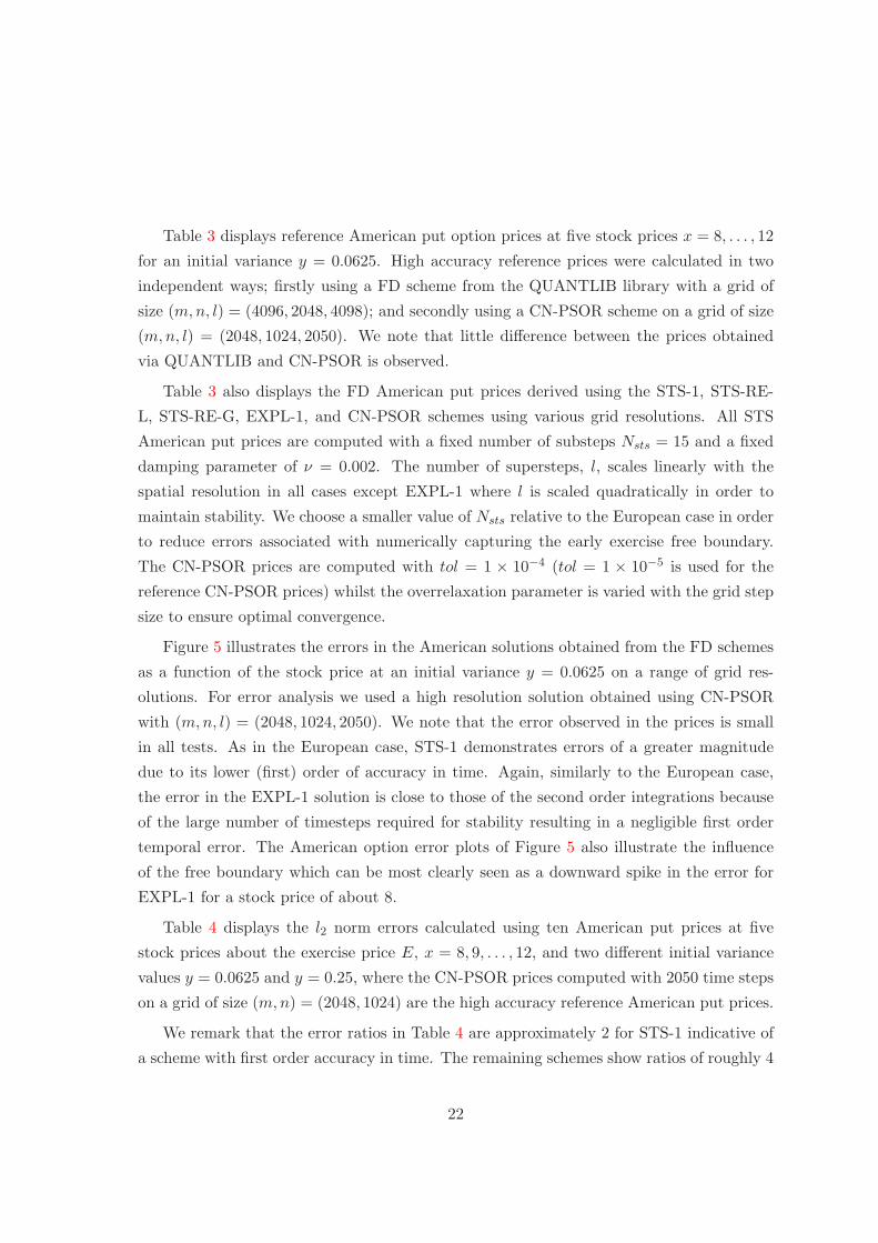
Table 3 displays reference American put option prices at five stock prices x = 8, . . . , 12

for an initial variance y = 0.0625. High accuracy reference prices were calculated in two

independent ways; firstly using a FD scheme from the QUANTLIB library with a grid of

size (m, n, l) = (4096, 2048, 4098); and secondly using a CN-PSOR scheme on a grid of size

(m, n, l) = (2048, 1024, 2050). We note that little difference between the prices obtained

via QUANTLIB and CN-PSOR is observed.

Table 3 also displays the FD American put prices derived using the STS-1, STS-RE-

L, STS-RE-G, EXPL-1, and CN-PSOR schemes using various grid resolutions. All STS

American put prices are computed with a fixed number of substeps Nsts = 15 and a fixed

damping parameter of ν = 0.002. The number of supersteps, l, scales linearly with the

spatial resolution in all cases except EXPL-1 where l is scaled quadratically in order to

maintain stability. We choose a smaller value of Nsts relative to the European case in order

to reduce errors associated with numerically capturing the early exercise free boundary.

The CN-PSOR prices are computed with tol = 1 × 10−4 (tol = 1 × 10−5 is used for the

reference CN-PSOR prices) whilst the overrelaxation parameter is varied with the grid step

size to ensure optimal convergence.

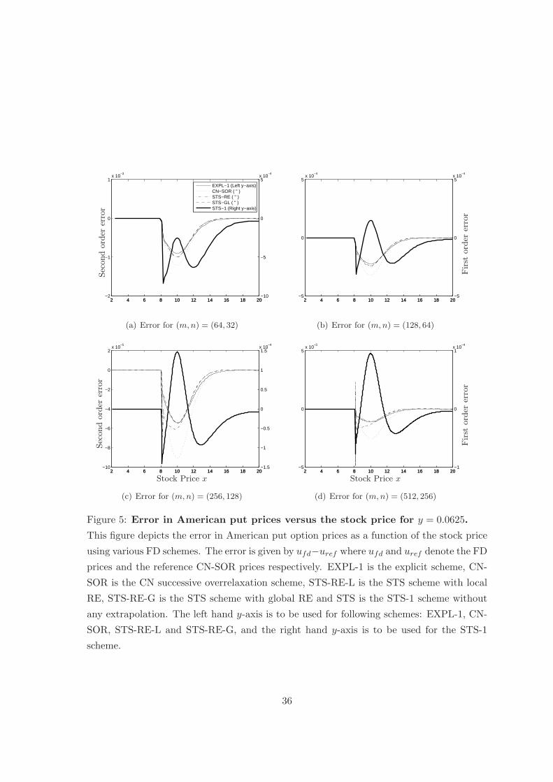
Figure 5 illustrates the errors in the American solutions obtained from the FD schemes

as a function of the stock price at an initial variance y = 0.0625 on a range of grid res-

olutions. For error analysis we used a high resolution solution obtained using CN-PSOR

with (m, n, l) = (2048, 1024, 2050). We note that the error observed in the prices is small

in all tests. As in the European case, STS-1 demonstrates errors of a greater magnitude

due to its lower (first) order of accuracy in time. Again, similarly to the European case,

the error in the EXPL-1 solution is close to those of the second order integrations because

of the large number of timesteps required for stability resulting in a negligible first order

temporal error. The American option error plots of Figure 5 also illustrate the influence

of the free boundary which can be most clearly seen as a downward spike in the error for

EXPL-1 for a stock price of about 8.

Table 4 displays the l2 norm errors calculated using ten American put prices at five

stock prices about the exercise price E, x = 8, 9, . . . , 12, and two different initial variance

values y = 0.0625 and y = 0.25, where the CN-PSOR prices computed with 2050 time steps

on a grid of size (m, n) = (2048, 1024) are the high accuracy reference American put prices.

We remark that the error ratios in Table 4 are approximately 2 for STS-1 indicative of

a scheme with first order accuracy in time. The remaining schemes show ratios of roughly 4

22

on successive doubling of spatial resolution suggesting second order accuracy in the leading

error terms. In all cases except EXPL-1 this is the expected behaviour for schemes of second

order accuracy in both space and time when the spatial and temporal errors are comparable

in magnitude. EXPL-1 has negligible temporal error and second order accuracy may only

be inferred in the spatial terms.

In terms of relative error magnitudes, the STS-1 method may be seen to have the largest

error followed by CN-PSOR. Furthermore, it is clear that the STS-2 methods have only

slightly larger errors relative to EXPL-1 despite the latter’s far greater, albeit first order

accurate, temporal resolution.

With regard to the CPU times also provided by table 4, we find that, similarly to the

European case, STS-2 schemes are faster than the CN-PSOR scheme and display lower

errors. Additionally, the STS-1 scheme is observed to be approximately three to four times

faster than the CN-PSOR scheme.

As a final exercise in validation, table 5 displays American put option prices at the

five stock prices x = 8, 9, . . . , 12 calculated with variances of y = 0.0625 and 0.25. Along

with the two reference prices from table 4, three sets of STS-RE-G prices are displayed

for a single spatial grid of size (m, n) = (2048, 1024) but different STS parameter settings.

We first set Nsts = 30, ν = 0.0006 and l = 2050, so that results are comparable to the

CN-PSOR results. We also examine two additional choices of parameter sets with Nsts =

25, ν = 0.0006, l = 2750 and Nsts = 35, ν = 0.0006, l = 1800. These results are compared

to the American put option prices published in the literature using the same sets of SV

parameters. We find that the American option prices from all three STS parameter settings

agree very closely with the reference prices and those prices in the literature. In particular,

agreement with prices quoted by Ikonen & Toivanen (2007b) is strong.

6 Conclusion

An acceleration technique, known as Super-Time-Stepping (STS), for explicit finite differ-

ence (FD) algorithms is introduced for the first time in the two-factor setting of stochastic

volatility. We demonstrate the efficacy of the method by pricing European and American

put options in a series of bench-tests with well-known FD techniques.

We demonstrate degrees of acceleration provided by the STS method which yield com-

parable, and even superior, efficiencies to implicit differencing methods. Of central impor-

23

tance, this is achieved with no significant increase in implementation complexity over and

above that of the underlying standard explicit algorithm.

Given that STS accelerated methods inherit the simplicity of explicit methods whilst

achieving high accuracy at low computational cost, we conclude that when faced with com-

plex numerical pricing problems, the approach presented here offers a compelling alternative

to conventional implicit techniques. Models involving multi-dimensional parameter spaces,

non-uniform meshes, moving boundaries, or meshes which are distributed in parallel over

several processors will be particularly amenable to STS accelerated explicit methods.

24

A Boundary Discretization

The following discretizations are used at the boundaries. At x0 we use a Dirichlet bound-

ary condition with u(x0, yj , τk) = exp (−rk∆t)max [E − x0, 0] for European options and

u(x0, yj , τk) = max [E − x0, 0] for American options. At xmax we use a Neumann condition

given by

∂um,j

∂x≈ aC

ll um−2,j + aCl um−1,j + aCum,j = 0,

⇒ um,j = − 1

aC

(

aCll um−2,j + aC

l um−1,j

)

,

where

aCll =

hr (xm−1)

hl (xm−1) (hl (xm−1) + hr (xm−1)),

aCl = − hl (xm−1) + hr (xm−1)

hl (xm−1)hr (xm−1),

aC =hl (xm−1) + 2hr (xm−1)

hr (xm−1) (hl (xm−1) + hr (xm−1)).

At ymax a Neumann condition is also used

∂ui,n

∂y≈ bC

ddui,n−2 + bCd ui,n−1 + bCui,n = 0,

⇒ ui,n = − 1

bC

(

bCddui,n−2 + bC

d ui,n−1

)

,

where

bCdd =

hu (yn−1)

hd (yn−1) (hd (yn−1) + hu (yn−1)),

bCd = − hd (yn−1) + hu (yn−1)

hd (yn−1)hu (yn−1),

bC =hd (yn−1) + 2hu (yn−1)

hu (yn−1) (hd (yn−1) + hu (yn−1)).

At y0 the value for ui,0 satisfies a reduced PDE and is solved explicitly or implicitly in the

same way as the solution to ui,j at the inner points on the grid. The PDE at y0 is given by

∂ui,0

∂τ− rxi

∂ui,0

∂x− αβ

∂ui,0

∂y+ rui,0 = 0,

⇒∂ui,0

∂τ− rxi

(

ui+1,0 − ui,0

hr (xi)

)

− αβ

(

ui,1 − ui,0

hu (y0)

)

+ rui,0 = 0.

25

B Upwinded Differencing

Recall from section 3.1 that the Heston PDE at a reference point u = uij can be written

as follows:

Lu =∂u

∂τ+ Au = 0,

in which A is a nine component operator matrix given by

A =

Alu Au Aru

Al Ac Ar

Ald Ad Ard

,

with

Ac = −(

1

2yx2aD + ργxycD +

1

2γ2ybD + rxaC + α (β − y) bC − r

)

,

Al = −(

1

2yx2aD

l + ργxycDl + rxaC

l

)

,

Ar = −(

1

2yx2aD

r + ργxycDr + rxaC

r

)

,

Ad = −(

frac12γ2ybDd + ργxycD

d + α (β − y) bCd

)

,

Au = −(

1

2γ2ybD

u + ργxycDu + α (β − y) bC

u

)

,

Ald = −ργxycDld, Alu = −ργxycD

lu

Ard = −ργxycDrd, Aru = −ργxycD

ru,

where the superscript D denotes diffusion terms and the superscript C denotes convection

terms defined in section 3.1. To adjust for upwinding we first define forward and backward

convection terms as follows:

aCFl = 0, aCF

r =1

hr, aCB

l = − 1

hl, aCB

r = 0,

bCFd = 0, bCF

u =1

hu, bCB

d = − 1

hd, aCB

r = 0.

26

At each point on the grid we adjust the nine component operator matrix A to implement

upwinding. For exampe Ac is adjusted as follows:

Auwc = −

(

1

2yx2aD + ργxycD +

1

2γ2ybD

+ rx[

aC1{Al<0,Ar<0} + aCFr 1{Al>0} + aCB

l 1{Ar>0}

]

+ α (β − y)[

bC1{Au<0,Ad<0} + bCFu 1{Ad>0} + bCB

d 1{Au>0}

]

− r)

.

Similarly we adjust the other convection components of the operator matrix A as follows:

aCl → aC

l 1{Al<0,Ar<0} + aCFl 1{Al>0} + aCB

l 1{Ar>0},

aCr → aC

r 1{Al<0,Ar<0} + aCFr 1{Al>0} + aCB

r 1{Ar>0},

bCd → bC

l 1{Ad<0,Au<0} + bCFd 1{Ad>0} + bCB

d 1{Au>0},

bCu → bC

u 1{Ad<0,Au<0} + bCFu 1{Ad>0} + bCB

u 1{Au>0}.

C Projected Successive OverRelaxation

PSOR is an important method for solving LCPs and is widely used to price American

options, see for example Tavella & Randall (2000); Wilmott et al. (1993). For completeness

we include a short description of the PSOR algorithm in this section of the appendix.

To solve the LCP in Eq 28 assume the solution u(k)ij is known at time k and we need

to determine the solution u(k+1)ij . For notional clarity denote uij = u

(k)ij and vij = u

(k+1)ij .

PSOR approximates the value vij to within a specified tolerance with the iterated solution

vs+1ij . The algorithm proceeds as follows:

1. Initialize unknown value with solution at previous time step i. e. v(0)ij = uij .

2. Perform the following sequence of iteration steps over s:

cv(s+1)i,j = (1 − ω) uij +

ω

Bi,i

Ci,juij −i−1∑

p=0

j−1∑

q=0

Bp,qv(s+1)p,q −

M∑

p=i+1

N∑

q=j+1

Bp,q v(s)p,q

,

v(s+1)i,j = max

[

cv(s+1)i,j , gi,j

]

, for i = 0, . . . , m, j = 0, . . . , n,

where cv(s)i,j denotes the approximated continuation value of the option at iteration s

and gij denoted the immediate exercise value of the option.

27

3. Do until∥

∥

∥v

(s+1)i,j − v

(s)i,j

∥

∥

∥≤ tol or until s = Imax, where tol is the tolerance level and

Imax is the maximum number of iterations.

4. Set u(k+1)ij = v

(s+1)i,j .

References

Alexiades, V., Amiez, G., and P. Gremaud, 1996, “Super-Time-Stepping acceleration of

explicit schemes for parabolic problems”, Com. Num. Meth. Eng., 12, 31-42.

Bates, D., 1973. “Jumps and Stochastic Volatility: Exchange Rate Processes Implicit in

Deutshe Mark Options”, Review of Financial Studies, 9, 69-107.

Black, F. and M.S. Scholes, 1973. “The pricing of options and corporate liabilities”, Journal

of Political Economy, 81, 637-654.

Brennan, M., and E. Schwartz, 1977. “The valuation of American put options”, Journal of

Finance, 32, 449-462.

Carr, P. and D. Madan, 1999. “Option valuation using the fast Fourier transform”, Journal

of Computational Finance 2, 61-73.

Clarke, N., and K. Parrot, 1999. “Multigrid for American option pricing with stochastic

volatility”, Applied Mathematical Finance, 177-195.

Cont, R. and P. Tankov, 2004. “Financial Modelling With Jump Processes”, Chapman &

Hall/CRC Financial Mathematics Series.

Crank, J., 1984. “Free and moving boundary problems”, Oxford: Clarendon Press.

C.W. Cryer, 1971. “The solution of a quadratic programming problem using systematic

overrelaxation”, SIAM Journal on Control, 9, 385-392.

Duffie, D., J. Pan, and K. Singleton (2000). Transform analysis and asset pricing for affine

jump-diffusions. Econometrica 68, 1343-76.

Evje, S., Karlsen, K. H., Risebro, N. H., 2001. “A continuous dependence result for nonlinear

degenerate parabolic equations with spatially dependent flux function”, in Int. Series of

Numerical Mathematics, Birkhauser-Verlag, 140, 337-346.

28

Gentzsch, W., 1979. “Numerical solution of linear and non-linear parabolic differential

equations by a time-discretisation of third order accuracy”, in Hirschel, E. H. (ed.),

Proceeding of the Third GAMM-Conference on Numerical Methods in Fluid Mechanics,

Friedr. Vieweg & Sohn, pp. 109-117.

Geske, R., and H.E. Johnson, 1984. “The American Put Option Valued Analytically.” The

Journal of Finance, 39, 1511-1524.

Heston, S.L., 1993. “A Closed-Form Solution for Options with Stochastic Volatility with

Applications to Bond and Currency Options”, The Review of Financial Studies, Vol. 6,

No. 2, pp. 327-343.

Kluge, T., 2002. “Pricing derivatives in stochastic volatility models using the finite difference

method”, Dimploma Thesis, Chemnitz University of Technology.

Kurpiel, A. and T. Roncalli, 2000. “Hopscotch Methods for Two State Financial Models”,

Journal of Computational Finance, Vol. 2/3, 2000.

Ikonen, S. and J. Toivanen, 2007a. “Componentwise splitting methods for pricing American

options under stochastic volatility”, International Journal of Theoretical and Applied

Finance, Vol. 10, No. 2, pp. 331-361.

Ikonen, S. and J. Toivanen, 2007b. “Efficient numerical methods for pricing American op-

tions under stochastic volatility”, Numerical Methods for Partial Differential Equations,

Vol. 24, Issue 1, 104-126.

Markoff, W., 1916. “Uber Polynome, die in einem gegebenen Intervalle moglichst wenig von

null abweichen”, Mathematische Annalen, 77, 213-258, translated by J. Grossman from

original Russian article published in 1892.

Merton, R.C., 1973. “The theory of rational option pricing”, Bell Journal of Economics

and Management Science, 4, 141-183.

Merton, R.C., 1976.“Option Pricing when the Underlying Returns are Discontinuous”.

Journal of Financial Economics 3, 125-144.

Mignone, A., Bodo, G., Massaglia, S., Matsakos, T., Tesileanu, O., Zanni, C., Ferrari, A.,

2007. “PLUTO: A Numerical Code for Computational Astrophysics”, ApJS, 170, 228

29

Nielsen, B.,Skavhaug,O. and A.Tveito, 2002. “Penalty and front-fixing methods for the

numerical solution of American option problems”, Journal of Computational Finance, 5.

Oosterlee, C.W. 2003. “On multigrid for linear complementarity problems with applications

to American-style options”, Electronic Transactions Numerical Analysis, 15, 165-185.

O’Sullivan, S., Downes, T. P., 2006. “An explicit scheme for multifluid magnetohydrody-

namics”, MNRAS, 366, 1329

O’Sullivan, S., Downes, T. P., 2007. “A three-dimensional numerical method for modelling

weakly ionized plasmas”, MNRAS, 376, 1648

O’Sullivan, S., O’Sullivan, C., 2010. “On the acceleration of explicit finite difference meth-

ods for option pricing”, forthcoming Quantitative Finance.

R. Rannacher, 1984. “Finite element solution of diffusion problems with irregular data”,

Numerical Mathematics, 43, 309-327.

Sbalzarini, I. F., Hayer, Helenius, A., Koumoutsakos, P., 2006. “Simulations of (an) isotropic

diffusion on curved biological surfaces”, Biophys. J., 90, 84788485.

Shi, Y., Li, L., Liang, C. H., 2006. “Multidomain pseudospectral time-domain algorithm

based on super-time-stepping method”, IEE Proceedings Microwaves, Antennas and

Propagation, 153, 55-60.

Sommeijer, B. P., Shampine, L. F., Verwer, J. G., 1997. “RKC: An explicit solver for

parabolic PDEs”, Technical Report MAS-R9715, CWI Amsterdam.

Tavella, D. and C. Randall, 2000. “Pricing financial instruments: the finite difference

method” John Wiley and Sons, New York.

van der Houwen, P. J., 1977. “Construction of integration formulas for initial value prob-

lems”, North-Holland, Amsterdam-New York.

van der Houwen, P. J., Sommeijer, B. P., 1980. “On the internal stability of explicit m-stage

Runge–Kutta methods for large values of m”, Z. Angew. Math. Mech., 60, 479-485.

Verwer, J. G., Hundsdorfer, W. H., Sommeijer, B. P., 1990. “Convergence Properties of the

Runge-Kutta-Chebyshev Method”, Numer. Math., 57, 157-178.

30

Verwer, J. G., 1996. “Explicit Runge-Kutta methods for parabolic partial differential equa-

tions”, Appl. Num. Math, 22, 359-379.

Wilmott, P., Howison, S. and Dewynne, J., 1995, “Option pricing: mathematical models

and computation”, Oxford Financial Press.

Winkler, G., Apel, T. and U. Wystup, 2001. “Valuation of options in Heston’s stochastic

volatility model using finite element methods”, Working Paper, Chemnitz University of

Technology.

Zvan, R., Forsyth, P.A. and Vetzal K.R., 1998. “Penalty methods for pricing American

options with stochastic volatility”, Journal of Computational and Applied Mathematics,

91, 199-218.

Zvan, R., Forsyth, P.A. and Vetzal K.R., 2003. “Negative coefficients in two-factor option

pricing models”, Journal of Computational Finance, 7, 37-73.

31

0 5 10 15 200.05

0.1

0.15

0.2

0.25

0.3

0.35

0.4

Non-u

niform

gri

dst

epsi

ze

Stock price

(a) Non-uniform grid step size in the x-direction

0 0.2 0.4 0.6 0.8 10

0.005

0.01

0.015

0.02

0.025

0.03

0.035

0.04

0.045

Non-u

niform

gri

dst

epsi

zeVariance

(b) Non-uniform grid step size in the y-direction

Figure 1: Grid step size as a function the stock price and variance.

These figures plot the stock price grid step size against the stock price and the variance grid

step size against the variance. The plots emphasise how the grid step size reduces around

areas of interest such as the exercise price or low variance values.

32

0 5 10 15 20 25 300

100

200

300

400

500

600

700

800

900

Ref line

ν = 5 × 10−1

ν = 5× 10−2

ν = 5× 10−3

ν = 5× 10−4

ν = 0

Acc

um

ula

ted

tim

ein

ST

S

Substeps: j = 1, . . . , Nsts

Figure 2: Illustration of acceleration via STS.

Figure 2 plots accumulated time,∑j

k=1 ∆τk, in STS versus the substep number j over a sin-

gle superstep ∆τsts with Nsts = 30 for a range of damping factors ν. The accumulated time

is plotted in units of the standard explicit timestep ∆τexpl. A reference line at Nsts∆τexpl

(= 30 in units of ∆τexpl) indicates the time attained over Nsts unaccelerated standard ex-

plicit steps. Note that acceleration approaches Nsts times this value as ν → 0, in agreement

with equation (38). Note also that deceleration occurs for the highest considered damping

factor of ν = 0.5.

33

0 0.2 0.4 0.6 0.8 1

x 10−3

70

80

90

100

110

120

130

140

150

160

No.

ofsu

per

step

sl

Damping parameter ν

(a) Number of supersteps l versus ν

−7 −6.5 −6 −5.5 −5 −4.5 −4 −3.5 −370

80

90

100

110

120

130

140

150

160

Num

ber

ofsu

per

step

sl

log10

ν

(b) Number of supersteps l versus log10

ν

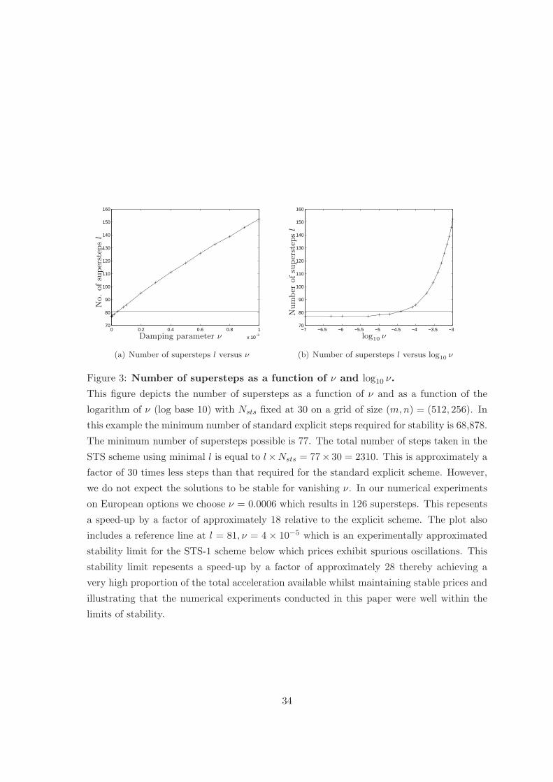
Figure 3: Number of supersteps as a function of ν and log10 ν.

This figure depicts the number of supersteps as a function of ν and as a function of the

logarithm of ν (log base 10) with Nsts fixed at 30 on a grid of size (m, n) = (512, 256). In

this example the minimum number of standard explicit steps required for stability is 68,878.

The minimum number of supersteps possible is 77. The total number of steps taken in the

STS scheme using minimal l is equal to l×Nsts = 77× 30 = 2310. This is approximately a

factor of 30 times less steps than that required for the standard explicit scheme. However,

we do not expect the solutions to be stable for vanishing ν. In our numerical experiments

on European options we choose ν = 0.0006 which results in 126 supersteps. This repesents

a speed-up by a factor of approximately 18 relative to the explicit scheme. The plot also

includes a reference line at l = 81, ν = 4 × 10−5 which is an experimentally approximated

stability limit for the STS-1 scheme below which prices exhibit spurious oscillations. This

stability limit repesents a speed-up by a factor of approximately 28 thereby achieving a

very high proportion of the total acceleration available whilst maintaining stable prices and

illustrating that the numerical experiments conducted in this paper were well within the

limits of stability.

34

2 4 6 8 10 12 14 16 18 20−12

−10

−8

−6

−4

−2

0

2

4x 10

−4

2 4 6 8 10 12 14 16 18 20−2.5

−2

−1.5

−1

−0.5

0

0.5

1

1.5x 10

−3

EXPL−1 (Left y−axis)CN−SOR ( " )STS−RE ( " )STS−GL ( " )STS−1 (Right y−axis)

Sec

ond

ord

erer

ror

(a) Error for (m, n) = (64, 32)

2 4 6 8 10 12 14 16 18 20−4

−2

0

2x 10

−4

2 4 6 8 10 12 14 16 18 20−2

−1

0

1x 10

−3

Fir

stord

erer

ror

(b) Error for (m, n) = (128, 64)

2 4 6 8 10 12 14 16 18 20−1

0

1x 10

−4

2 4 6 8 10 12 14 16 18 20−1

0

1x 10

−3

Sec

ond

ord

erer

ror

Stock Price x

(c) Error for (m, n) = (256, 128)

2 4 6 8 10 12 14 16 18 20−2

0

2x 10

−5

2 4 6 8 10 12 14 16 18 20−5

0

5x 10

−4

Fir

stord

erer

ror

Stock Price x

(d) Error for (m, n) = (512, 256)

Figure 4: Error in European put prices versus the stock price for y = 0.0625.

This figure depicts the error in European put option prices as a function of the stock price

using various FD schemes. The error is given by ufd−uref where ufd and uref denote the FD

prices and the reference CN-SOR prices respectively. EXPL-1 is the explicit scheme, CN-

SOR is the CN successive overrelaxation scheme, STS-RE-L is the STS scheme with local

RE, STS-RE-G is the STS scheme with global RE and STS is the STS-1 scheme without

any extrapolation. The left hand y-axis is to be used for following schemes: EXPL-1, CN-

SOR, STS-RE-L and STS-RE-G, and the right hand y-axis is to be used for the STS-1

scheme.

35

2 4 6 8 10 12 14 16 18 20−2

−1

0

1x 10

−3

2 4 6 8 10 12 14 16 18 20−10

−5

0

5x 10

−4

EXPL−1 (Left y−axis)CN−SOR ( " )STS−RE ( " )STS−GL ( " )STS−1 (Right y−axis)

Sec

ond

ord

erer

ror

(a) Error for (m, n) = (64, 32)

2 4 6 8 10 12 14 16 18 20−5

0

5x 10

−4

2 4 6 8 10 12 14 16 18 20−5

0

5x 10

−4

Fir

stord

erer

ror

(b) Error for (m, n) = (128, 64)

2 4 6 8 10 12 14 16 18 20−10

−8

−6

−4

−2

0

2x 10

−5

2 4 6 8 10 12 14 16 18 20−1.5

−1

−0.5

0

0.5

1

1.5x 10

−4

Sec

ond

ord

erer

ror

Stock Price x

(c) Error for (m, n) = (256, 128)

2 4 6 8 10 12 14 16 18 20−5

0

5x 10

−5

2 4 6 8 10 12 14 16 18 20−1

0

1x 10

−4

Fir

stord

erer

ror

Stock Price x

(d) Error for (m, n) = (512, 256)

Figure 5: Error in American put prices versus the stock price for y = 0.0625.

This figure depicts the error in American put option prices as a function of the stock price

using various FD schemes. The error is given by ufd−uref where ufd and uref denote the FD

prices and the reference CN-SOR prices respectively. EXPL-1 is the explicit scheme, CN-

SOR is the CN successive overrelaxation scheme, STS-RE-L is the STS scheme with local

RE, STS-RE-G is the STS scheme with global RE and STS is the STS-1 scheme without

any extrapolation. The left hand y-axis is to be used for following schemes: EXPL-1, CN-

SOR, STS-RE-L and STS-RE-G, and the right hand y-axis is to be used for the STS-1

scheme.

36

Table 1: European put prices evaluated using stock prices x = 8, 9, . . . , 12 and an initial

variance value of y = 0.0625 with STS parameters of ν = 0.0006 and Nsts = 30.

x

Method Grid (m, n, l) 8 9 10 11 12

Reference (FFT) 1.838868 1.048347 0.501465 0.208187 0.080428

Reference (CN-SOR) (2048, 1024, 2050) 1.838868 1.048347 0.501465 0.208186 0.080428

STS-1 (64, 32, 18) 1.837355 1.048321 0.502606 0.208727 0.079657

(128, 64, 34) 1.837830 1.048418 0.502317 0.208617 0.079983

(256, 128, 66) 1.838343 1.048341 0.501963 0.208402 0.080225

(512, 256, 130) 1.838598 1.048352 0.501733 0.208306 0.080328

STS-RE-L (64, 32, 18) 1.839445 1.048331 0.500517 0.207842 0.080441

(128, 64, 34) 1.838916 1.048414 0.501228 0.208148 0.080381

(256, 128, 66) 1.838895 1.048337 0.501406 0.208159 0.080425

(512, 256, 130) 1.838877 1.048349 0.501451 0.208183 0.080429

STS-RE-G (64, 32, 18) 1.839424 1.048301 0.500535 0.207825 0.080415

(128, 64, 34) 1.838910 1.048406 0.501232 0.208143 0.080374

(256, 128, 66) 1.838894 1.048335 0.501407 0.208158 0.080423

(512, 256, 130) 1.838877 1.048349 0.501451 0.208183 0.080428

EXPL-1 (64, 32, 1064) 1.839334 1.048302 0.500611 0.207860 0.080379

(128, 64, 4284) 1.838887 1.048407 0.501252 0.208152 0.080364

(256, 128, 17192) 1.838888 1.048335 0.501412 0.208161 0.080421

(512, 256, 68878) 1.838875 1.048349 0.501452 0.208183 0.080428

Grid (m, n, l, iterav, w)

CN-SOR (64, 32, 18, 22.3, 1.59) 1.839586 1.048240 0.500295 0.207683 0.080432

(128, 64, 34, 28.6, 1.75) 1.838951 1.048393 0.501177 0.208110 0.080378

(256, 128, 66, 35.5, 1.84) 1.838904 1.048331 0.501393 0.208150 0.080424

(512, 256, 130, 50.4, 1.87) 1.838879 1.048348 0.501448 0.208181 0.080429

37

Table 2: The (l2-norm) errors calculated using ten European put prices at stock prices of

x = 8, 9, . . . , 12, and initial variance values of y = 0.0625 and 0.25. Also reported are the

the ratio of consective errors, and the CPU times in seconds.

Method Grid (m, n, l) Error Ratio CPU

STS-1 (64, 32, 18) 0.005124 0.07

(128, 64, 34) 0.003068 1.67 0.30

(256, 128, 66) 0.001620 1.89 2.48

(512, 256, 130) 0.000845 1.92 24.54

STS-RE-L (64, 32, 18) 0.001657 0.22

(128, 64, 34) 0.000365 4.54 0.90

(256, 128, 66) 0.000101 3.60 7.45

(512, 256, 130) 0.000023 4.37 69.80

STS-RE-G (64, 32, 18) 0.001543 0.24

(128, 64, 34) 0.000348 4.43 0.99

(256, 128, 66) 0.000097 3.59 8.23

(512, 256, 130) 0.000022 4.42 89.87

EXPL-1 (64, 32, 1064) 0.001341 0.14

(128, 64, 4284) 0.000298 4.50 1.25

(256, 128, 17192) 0.000078 3.79 22.16

(512, 256, 68878) 0.000021 3.65 452.76

Grid (m, n, l, iterav, w)

CN-SOR (64, 32, 18, 22.3, 1.59) 0.002085 0.39

(128, 64, 34, 28.6, 1.75) 0.000473 4.41 2.26

(256, 128, 66, 35.5, 1.84) 0.000131 3.61 15.24

(512, 256, 130, 50.4, 1.87) 0.000030 4.36 129.61

38

Table 3: American put prices evaluated using stock prices x = 8, 9, . . . , 12 and an initial

variance value of y = 0.0625 with STS parameters of ν = 0.002 and Nsts = 15.

x

Method Grid (m, n, l) 8 9 10 11 12

Reference (Quantlib) (4096, 2048, 4098) 2.000000 1.107611 0.520024 0.213675 0.082043

Reference (CN-PSOR) (2048, 1024, 2050) 2.000000 1.107620 0.520030 0.213676 0.082043

STS-1 (64, 32, 66) 2.000000 1.107834 0.519776 0.213609 0.081817

(128, 64, 130) 2.000000 1.107836 0.520177 0.213805 0.081892

(256, 128, 258) 2.000000 1.107677 0.520176 0.213742 0.081996

(512, 256, 514) 2.000000 1.107662 0.520125 0.213725 0.082025

STS-RE-L (64, 32, 66) 2.000000 1.107601 0.519038 0.213308 0.082022

(128, 64, 130) 2.000000 1.107700 0.519787 0.213639 0.081988

(256, 128, 260) 2.000000 1.107599 0.519970 0.213651 0.082040

(512, 256, 514) 2.000000 1.107619 0.520016 0.213675 0.082045

STS-RE-G (64, 32, 66) 2.000000 1.107600 0.519033 0.213300 0.082016

(128, 64, 130) 2.000000 1.107712 0.519788 0.213636 0.081985

(256, 128, 258) 2.000000 1.107614 0.519975 0.213651 0.082039

(512, 256, 514) 2.000000 1.107626 0.520019 0.213675 0.082045

EXPL-1 (64, 32, 1064) 2.000000 1.107652 0.519126 0.213336 0.081992

(128, 64, 4284) 2.000000 1.107719 0.519804 0.213640 0.081977

(256, 128, 17192) 2.000000 1.107612 0.519975 0.213650 0.082036

(512, 256, 68878) 2.000000 1.107625 0.520018 0.213674 0.082044

Grid (m, n, l, iter-avg, w)

CN-PSOR (64, 32, 66, 9.8, 1.60) 2.000000 1.107465 0.518820 0.213154 0.081951

(128, 64, 130, 13.5, 1.75) 2.000000 1.107656 0.519707 0.213577 0.081956

(256, 128, 258, 18.8, 1.84) 2.000000 1.107589 0.519939 0.213624 0.082025

(512, 256, 514, 23.4, 1.87) 2.000000 1.107616 0.520004 0.213664 0.082038

39

Table 4: The (l2-norm) errors calculated using ten American put prices at stock prices of

x = 8, 9, . . . , 12, and initial variance values of y = 0.0625 and 0.25. Also reported are the

the ratio of consective errors, and the CPU times in seconds.

Method Grid (m, n, l) Error Ratio CPU

STS-1 (64, 32, 66) 0.001091 0.18

(128, 64, 130) 0.000784 1.39 0.58

(256, 128, 260) 0.000445 1.76 4.90

(512, 256, 514) 0.000262 1.70 38.53

STS-RE-L (64, 32, 66) 0.001521 0.49

(128, 64, 130) 0.000360 4.22 1.76

(256, 128, 258) 0.000098 3.69 14.84

(512, 256, 514) 0.000019 5.22 119.74

STS-RE-G (64, 32, 66) 0.001531 0.44

(128, 64, 130) 0.000358 4.27 1.74

(256, 128, 258) 0.000086 4.17 14.62

(512, 256, 514) 0.000018 4.86 118.02

EXPL-1 (64, 32, 1064) 0.001351 0.46

(128, 64, 4284) 0.000329 4.10 1.70

(256, 128, 17192) 0.000083 3.95 27.04

(512, 256, 68878) 0.000017 4.81 452.48

Grid (m, n, l, iter-avg, w)

CN-PSOR (64, 32, 66, 9.8, 1.60) 0.001885 0.96

(128, 64, 130, 13.5, 1.75) 0.000501 3.76 3.44

(256, 128, 258, 18.8, 1.84) 0.000160 3.14 28.00

(512, 256, 514, 23.4, 1.87) 0.000042 3.81 226.95

40

Table 5: American put reference prices calculated using the STS-RE-G and CN-PSOR

schemes at various stock prices, x, and for two initial variances: y = 0.0625, 0.25 on a grid

of size (m, n, l). These price are compared to benchmark prices computed using code from

quantlib, a freeware financial software resource. Other reference prices published in the

literature are also included.

x

Reference y 8 9 10 11 12

STS-RE-G m = 2048, n = 1024, l = 2050 0.0625 2.000000 1.107622 0.520032 0.213678 0.082044

Nsts = 30, ν = 0.0006 0.25 2.078364 1.333633 0.795977 0.448273 0.242811

STS-RE-G m = 2048, n = 1024, l = 2750 0.0625 2.000000 1.107622 0.520032 0.213678 0.082044

Nsts = 25, ν = 0.0006 0.25 2.078364 1.333633 0.795977 0.448273 0.242810

STS-RE-G m = 2048, n = 1024, l = 1800 0.0625 2.000000 1.107622 0.520032 0.213678 0.082044

Nsts = 35, ν = 0.0006 0.25 2.078357 1.333623 0.795967 0.448264 0.242803

STS-RE-G m = 2048, n = 1024, l = 1600 0.0625 2.000000 1.107622 0.520032 0.213678 0.082045

Nsts = 30, ν = 0.0002 0.25 2.078364 1.333633 0.795977 0.448274 0.242811

STS-RE-G m = 2048, n = 1024, l = 1400 0.0625 2.000000 1.107622 0.520033 0.213678 0.082045

Nsts = 30, ν = 0.00005 0.25 2.078364 1.333633 0.795977 0.448274 0.242811

CN-PSOR m = 2048, n = 1024, l = 2050 0.0625 2.000000 1.107620 0.520030 0.213676 0.082043

tol = 1 × 10−5, w = 1.85 0.25 2.078363 1.333631 0.795974 0.448271 0.242809

Quantlib m = 4096, n = 2048, l = 4098 0.0625 2.000000 1.107611 0.520024 0.213675 0.082043

0.25 2.078355 1.333626 0.795972 0.448271 0.242803

Ikonen & Toivanen (2007b) 0.0625 2.000000 1.107629 0.520038 0.213681 0.082046

0.25 2.078372 1.333640 0.795983 0.448277 0.242813

Clarke & Parrot (1999) 0.0625 2.0000 1.1080 0.5316 0.2261 0.0907

0.25 2.0733 1.3290 0.7992 0.4536 0.2502

Zvan et al. (1998) 0.0625 2.0000 1.1076 0.5202 0.2138 0.0821

0.25 2.0784 1.3337 0.7961 0.4483 0.2428

Oosterlee (2003) 0.0625 2.000 1.107 0.517 0.212 0.815

0.25 2.079 1.334 0.796 0.449 0.24341