pricing barrier options with numerical methods · pricing barrier options with numerical methods...
TRANSCRIPT
Pricing barrier options with numerical methods
C.N de Ponte
Dissertation submitted in partial fulfilment of therequirements for the degree Master of Science in Applied
Mathematics at the Potchefstroom campus of theNorth-WestUniversity
Supervisor : Dr E.H.A Venter
The financial assistance of the National Research Foundation (NRF) towards this research is
hereby acknowledged. Opinions expressed and conclusions arrived at, are those of the author
and are not necessarily to be attributed to the NRF.
ii
Abstract
Barrier options are becoming more popular, mainly due to the reduced cost to hold a
barrier option when compared to holding a standard call/put options, but exotic options
are difficult to price since the payoff functions depend on the whole path of the underlying
process, rather than on its value at a specific time instant.
It is a path dependent option, which implies that the payoff depends on the path followed by
the price of the underlying asset, meaning that barrier options prices are especially sensitive
to volatility.
For basic exchange traded options, analytical prices, based on the Black-Scholes formula,
can be computed. These prices are influenced by supply and demand. There is not always
an analytical solution for an exotic option. Hence it is advantageous to have methods that
efficiently provide accurate numerical solutions. This study gives a literature overview and
compares implementation of some available numerical methods applied to barrier options.
The three numerical methods that will be adapted and compared for the pricing of barrier
options are:
� Binomial Tree Methods
� Monte-Carlo Methods
� Finite Difference Methods

iii
Key terms
� Barrier options
� Black-Scholes
� Binomial method
� Trinomial method
� Monte Carlo simulation
� Finite difference method
iv
Summary
Barrier options are probably the oldest of all exotic options and have been traded in the US
market since 1967. The most popular standard barrier options are knock-out and knock-in
options. In 1973 Merton provided the first analytical formula to price basic barrier options
in continuous time.
Most real-world financial barrier options pricing have no analytical solutions, because the
barrier structure is complex or discrete. There are essentially no analytical formulas for
pricing discrete barrier options, and numerical pricing is difficult and slow to converge.
This dissertation offers a discussion of the theoretical background of different barrier op-
tions, an investigation of numerical techniques to determine the value of a barrier option, a
description of the algorithms and shows the implementation of the algorithms in MATLAB
code.
A thorough literature study was undertaken to investigate the current available pricing
techniques, after which MATLAB code was implemented and experimented, with numer-
ical data. The efficiency of the numerical methods and adaptive methods used in the
valuation of financial derivatives, with special focus on barrier options was studied. Numer-
ical methods studied include binomial methods, Monte Carlo Methods and finite difference
methods. The option price was obtained using the numerical methods and was compared
to the analytical solution (if it existed).
The best lattice method is the adaptation of the trinomial method using the stretch tech-
nique. The Monte Carlo method converges very slowly to obtain an accurate value, whilst
the Crank-Nicolson finite difference method takes the least number of time steps to obtain
an accurate value.

v
Declaration
I declare that, apart from the assistance acknowledged, the research presented in this dis-
sertation is my own unaided work. It is being submitted in partial fulfilment of the re-
quirements for the degree Master of Science in Applied Mathematics at the Potchefstroom
campus of the North-West University. It has not been submitted before for any degree or
examination to any other University.
Nobody, including Dr. Venter, but myself is responsible for the final version of this disser-
tation.
Signature.................................
Date......................................
vi
Acknowledgements
Firstly, I’d like to thank my supervisor, Dr. Venter for her guidance, sugges-
tions, patience and assistance.
Next, I’d like to thank my parents, my brother Christopher, my sister Caitlyn
and my boyfriend Paulo Oliveira. Their support, encouragement, love and pa-
tience through the tough and good times of writing this dissertation will always
be appreciated.
I thank the North West University (Potchefstroom) and the NRF for their fi-
nancial assistance, and Christien Terblanche for the language editing.

vii
Basic Notations
K - exercise/strike price
St - asset price at general time
ST - asset price at expiry date
t - general time
T - expiry date
T − t - time to maturity
ct - payoff of European call option
pt - payoff of European put option
r - risk-free interest rate
σ - volatility
B - barrier
q - dividend yield
µ - drift
N(x) - Cumulative distribution function of the standard normal distribution
M - number of asset paths sampled
Smax - suitably large asset price
Contents
1 Introduction 1
2 Introduction to Options 3
2.1 Fundamental concepts of options . . . . . . . . . . . . . . . . . . . . . . . . 3
2.1.1 Definition of an option . . . . . . . . . . . . . . . . . . . . . . . . . . 3
2.1.2 Payoff of the option . . . . . . . . . . . . . . . . . . . . . . . . . . . 5
2.1.3 Factors affecting option prices . . . . . . . . . . . . . . . . . . . . . . 5
2.2 Black-Scholes . . . . . . . . . . . . . . . . . . . . . . . . . . . . . . . . . . . 7
2.2.1 Random variable and stochastic processes . . . . . . . . . . . . . . . 7
2.2.2 Asset price modelling . . . . . . . . . . . . . . . . . . . . . . . . . . 7
2.2.3 Ito’s lemma . . . . . . . . . . . . . . . . . . . . . . . . . . . . . . . . 8
2.2.4 The Black-Scholes model . . . . . . . . . . . . . . . . . . . . . . . . 9
3 Theory of Barrier Options 13
3.1 Characteristics of barrier options . . . . . . . . . . . . . . . . . . . . . . . . 13
3.2 Black-Scholes and barrier option pricing . . . . . . . . . . . . . . . . . . . . 16
4 Binomial and Trinomial Method 26
4.1 Binomial method . . . . . . . . . . . . . . . . . . . . . . . . . . . . . . . . . 26
4.1.1 Accuracy of option value . . . . . . . . . . . . . . . . . . . . . . . . 38
4.2 Trinomial method . . . . . . . . . . . . . . . . . . . . . . . . . . . . . . . . 39
4.3 Barrier options for the binomial and trinomial method . . . . . . . . . . . . 43
4.3.1 Direct barrier method . . . . . . . . . . . . . . . . . . . . . . . . . . 46
4.3.2 Errors with the binomial method for a barrier option . . . . . . . . . 48
4.3.3 A comparison of parameters for the trinomial method . . . . . . . . 49
4.3.4 Revised binomial model . . . . . . . . . . . . . . . . . . . . . . . . . 51
4.3.5 Interpolation technique . . . . . . . . . . . . . . . . . . . . . . . . . 53
viii
CONTENTS ix
4.3.6 Stretch technique . . . . . . . . . . . . . . . . . . . . . . . . . . . . . 57
4.3.7 A numerical comparison of a down-and-out call option using various techniques 59
4.4 Discrete barrier options . . . . . . . . . . . . . . . . . . . . . . . . . . . . . 61
4.4.1 The barrier adjustment technique for Black-Scholes . . . . . . . . . . 61
4.4.2 The barrier adjustment technique for the trinomial method . . . . . 63
5 Monte Carlo Method 66
5.1 Monte Carlo simulation . . . . . . . . . . . . . . . . . . . . . . . . . . . . . 66
5.1.1 Advantages of Monte Carlo . . . . . . . . . . . . . . . . . . . . . . . 69
5.1.2 Disadvantages of Monte Carlo . . . . . . . . . . . . . . . . . . . . . . 69
5.2 Barrier options . . . . . . . . . . . . . . . . . . . . . . . . . . . . . . . . . . 70
5.3 Variance reduction . . . . . . . . . . . . . . . . . . . . . . . . . . . . . . . . 72
5.3.1 Antithetic variates . . . . . . . . . . . . . . . . . . . . . . . . . . . . 72
5.3.2 Comparison . . . . . . . . . . . . . . . . . . . . . . . . . . . . . . . . 74
6 Finite Difference Methods 76
6.1 Explicit method . . . . . . . . . . . . . . . . . . . . . . . . . . . . . . . . . . 80
6.2 Implicit method . . . . . . . . . . . . . . . . . . . . . . . . . . . . . . . . . . 81
6.3 Crank-Nicolson method . . . . . . . . . . . . . . . . . . . . . . . . . . . . . 82
6.4 Barrier options . . . . . . . . . . . . . . . . . . . . . . . . . . . . . . . . . . 86
7 Conclusion 89
8 Appendix 92
8.1 Matlab code . . . . . . . . . . . . . . . . . . . . . . . . . . . . . . . . . . . . 92
8.1.1 Black-Scholes for barrier options . . . . . . . . . . . . . . . . . . . . 92
8.1.2 Standard options . . . . . . . . . . . . . . . . . . . . . . . . . . . . . 93
8.1.2.1 Binomial method . . . . . . . . . . . . . . . . . . . . . . . 93
8.1.2.2 Accuracy of option value . . . . . . . . . . . . . . . . . . . 94
8.1.2.3 Trinomial method . . . . . . . . . . . . . . . . . . . . . . . 96
8.1.3 Barrier options . . . . . . . . . . . . . . . . . . . . . . . . . . . . . . 97
8.1.3.1 Binomial method . . . . . . . . . . . . . . . . . . . . . . . 97
8.1.3.2 Trinomial method . . . . . . . . . . . . . . . . . . . . . . . 99
8.1.4 Interpolation technique . . . . . . . . . . . . . . . . . . . . . . . . . 101
8.1.5 Stretch technique . . . . . . . . . . . . . . . . . . . . . . . . . . . . . 103
8.1.6 Monte Carlo method . . . . . . . . . . . . . . . . . . . . . . . . . . . 105

CONTENTS x
8.1.7 Antithetic variable technique . . . . . . . . . . . . . . . . . . . . . . 106
8.1.8 Crank-Nicolson method . . . . . . . . . . . . . . . . . . . . . . . . . 107
Chapter 1
Introduction
Options are part of derivatives instruments. Derivatives are financial instruments that de-
rive their value from the value of other, more basic, underlying variables. These underlying
variables are stochastic, i.e. random, thus taking a position in a financial instrument built
on these random variables implies risk. This explains why one needs to have the correct
price for a given financial product if one does not want to take inconsiderate risks.
Exotic options are not a strict defined class of options, but rather refer to options with more
complicated properties than ordinary put and call options. Exotic options are usually born
of the particular needs of hedgers and investors using the instruments to manage financial
risk.
Barrier options are probably the oldest of all exotic options and have been traded in the
US market since 1967 (Chriss 1997, 462). They are extensions of a standard stock option.
Standard calls and puts have payoffs that depend on one predetermined value, the strike K,
whereas barrier options have payoffs that depend on two predetermined values namely the
strike K and the barrier B. The most popular standard barrier options are ’knock-out’ and
’knock-in’ options. A knock-in option is a contract that becomes active only when a certain
price is reached. A knock-out option is a contract that starts out as ordinary call or put
options, but they become null and void if the spot price ever crosses a certain predetermined
knock-out barrier. A major reason for the popularity of barrier options is that, because
there is a positive probability (in either case) of worthlessness, these options are cheaper
than the corresponding standard stock option, and hence possibly more attractive to the
speculator. They are also used by investors to gain exposure to future market scenarios
more complex than can be described by standard options.
In 1973 Merton provided the first analytical formula to price basic barrier options in con-
tinuous time. It is common practice to assume that the underlying asset is continuously
1
2
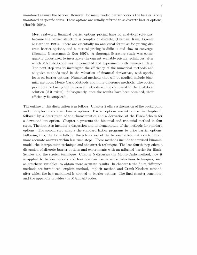
monitored against the barrier. However, for many traded barrier options the barrier is only
monitored at specific dates. These options are usually referred to as discrete barrier options,
(Horfelt 2003).
Most real-world financial barrier options pricing have no analytical solutions,
because the barrier structure is complex or discrete, (Derman, Kani, Ergener
& Bardhan 1995). There are essentially no analytical formulas for pricing dis-
crete barrier options, and numerical pricing is difficult and slow to converge,
(Broadie, Glasserman & Kou 1997). A thorough literature study was conse-
quently undertaken to investigate the current available pricing techniques, after
which MATLAB code was implemented and experiment with numerical data.
The next step was to investigate the efficiency of the numerical methods and
adaptive methods used in the valuation of financial derivatives, with special
focus on barrier options. Numerical methods that will be studied include bino-
mial methods, Monte Carlo Methods and finite difference methods. The option
price obtained using the numerical methods will be compared to the analytical
solution (if it exists). Subsequently, once the results have been obtained, their
efficiency is compared.
The outline of this dissertation is as follows. Chapter 2 offers a discussion of the background
and principles of standard barrier options. Barrier options are introduced in chapter 3,
followed by a description of the characteristics and a derivation of the Black-Scholes for
a down-and-out option. Chapter 4 presents the binomial and trinomial method in four
steps. The first step includes a discussion and implementation of the methods for standard
options. The second step adapts the standard lattice programs to price barrier options.
Following this, the focus falls on the adaptation of the barrier lattice methods to obtain
more accurate answers within less time steps. These methods include the revised binomial
model, the interpolation technique and the stretch technique. The last fourth step offers a
discussion of discrete barrier options and experiments with an adjusted barrier for Black-
Scholes and the stretch technique. Chapter 5 discusses the Monte-Carlo method, how it
is applied to barrier options and how one can use variance reductions techniques, such
as antithetic variables, to obtain more accurate results. In chapter 6 the finite difference
methods are introduced; explicit method, implicit method and Crank-Nicolson method,
after which the last mentioned is applied to barrier options. The final chapter concludes,
and the appendix provides the MATLAB codes.

Chapter 2
Introduction to Options
2.1 Fundamental concepts of options
Trading on options on an organized exchange started in the early 1980s (Hull 2000, 10).
They have two primary uses: speculation and hedging. The pricing of options is a topic of
some significance and interest due to their importance in financial markets. Standard option
contracts are traded on option exchanges, and their prices are widely listed. However, there
is also a market for more specialized option contracts such as exotic options, which are
designed to tailor to more specific risk management strategies.
2.1.1 Definition of an option
Options are a class of derivatives, i.e., financial assets of which the value depends on another
asset, called the underlying. The underlying can also be a non-financial asset, such as a
commodity, or an arbitrary quantity representing a risk factor to someone, such as weather,
so that setting up a market to transfer risks makes sense. Options are contracts with very
specific rules for issuing, trading and accounting (Brandimarte 2006, 35).
Options are contracts that give their holders the right to buy or sell an underlying asset at
a fixed price (called the strike, and denoted K) at a certain time in the future (the expiry
date, denoted T). The holder of an option pays an agreement fee (premium) at the start of
the option. The profit at time t = T is then equal to the payoff minus the premium.
The writer of the option keeps the premium regardless of whether or not the option is ulti-
mately exercised. It is paid by the buyer to the writer in order to enjoy the choice conferred
by holding the option. The writer has no such choice, but must trade if the buyer wishes
to do so.
3
CHAPTER 2. INTRODUCTION TO OPTIONS 4
All options of the same type (call or puts) are referred to as an option class where the call
and put is defined as:
• The call option gives the holder the right to buy the underlying asset by a certain date
for a certain price.
• The put option gives the holder the right to sell the underlying asset by a certain date for
a certain price.
If you own a call option you want the asset to rise as much as possible so that you can buy
the stock for a relatively small amount, then sell it and make a profit. When you own a put
option you want the asset price to fall as low as possible because the lower the asset price
at expiry the higher the profit.
An important relationship between the call and put is called the put-call parity
c− p = S −Ke−r(T−t). (2.1)
It shows that the value of a European call with a certain exercise price and exercise date
can be deduced from the value of a European put with the same exercise price and exercise
date, and vice versa. It is an important equation, because if (2.1) does not hold then there
are arbitrage opportunities (Hull 2000, 174).
The buyer of an option does not buy the underlying instrument; he or she buys a right. If
this right can be exercised only at the expiration date, then the option is European. If it
can be exercised any time during the specified period, the option is said to be American.
A Bermudan option is in between, given that it can be exercised at more than one of the
dates during the life of the option.
In the case of a European call, the option holder has purchased the right to ”buy” the
underlying instrument at a certain price, strike price, at a specific date, the expiration date.
In the case of European put, the option holder has again purchased the right to an action.
The action in this case is to ”sell” the underlying instrument at the strike price and at the
expiration date.
American style options can be exercised anytime until expiration and hence may be more
expensive. They may carry an early exercise premium. At the expiration date, options
cease to exist (Neftci 2008, 206).
There are two sides to every option contract. On one side is the investor who has taken the
long position (i.e., has bought the option), on the other side is the investor who has taken
a short position (i.e., has sold or written the option) (Hull 2000, 1).
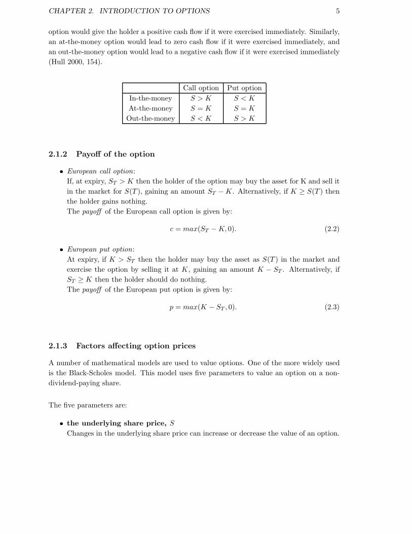
Options are referred to as in the money, at the money or out of the money. An in-the-money
CHAPTER 2. INTRODUCTION TO OPTIONS 5
option would give the holder a positive cash flow if it were exercised immediately. Similarly,
an at-the-money option would lead to zero cash flow if it were exercised immediately, and
an out-the-money option would lead to a negative cash flow if it were exercised immediately
(Hull 2000, 154).
Call option Put option
In-the-money S > K S < K
At-the-money S = K S = K
Out-the-money S < K S > K
2.1.2 Payoff of the option
� European call option:
If, at expiry, ST > K then the holder of the option may buy the asset for K and sell it
in the market for S(T ), gaining an amount ST −K. Alternatively, if K ≥ S(T ) then
the holder gains nothing.
The payoff of the European call option is given by:
c = max(ST −K, 0). (2.2)
� European put option:
At expiry, if K > ST then the holder may buy the asset as S(T ) in the market and
exercise the option by selling it at K, gaining an amount K − ST . Alternatively, if
ST ≥ K then the holder should do nothing.
The payoff of the European put option is given by:
p = max(K − ST , 0). (2.3)
2.1.3 Factors affecting option prices
A number of mathematical models are used to value options. One of the more widely used
is the Black-Scholes model. This model uses five parameters to value an option on a non-
dividend-paying share.
The five parameters are:
� the underlying share price, S
Changes in the underlying share price can increase or decrease the value of an option.

CHAPTER 2. INTRODUCTION TO OPTIONS 6
These price changes have opposite effects on calls and puts. For instance, as the value
of the underlying share price rises, call will generally increase and the value of a put
will generally decrease in price. A decrease in the underlying share price will generally
have the opposite effect.
� the strike price, K
The strike price determines whether or not an option has any intrinsic value. An
option’s premium (intrinsic value plus time value) generally increases as the option
becomes further in the money, and decreases as the option becomes more deeply out
of the money.
� the time to expiry, T-t
Time until expiration affects the time value component of an option’s premium. Gen-
erally, as expiration approaches, the levels of an option’s time value, for both puts and
calls, decreases or ”erodes”. This effect is most noticeable with at-the-money options.
� the volatility of the underlying share, σ
The value of an option will increase with the volatility of the underlying share.
� the risk-free interest rate, r
The effect of the risk-free interest rate has a small but measurable effect on option
premiums. This effect reflects the ”cost of carry” of shares in an underlying security,
the interest that might be paid for margin or received from alternative investments.
In the case of a dividend-paying share, dividends can be considered a sixth factor. The
price of an option is the premium paid at the outset.
CHAPTER 2. INTRODUCTION TO OPTIONS 7
2.2 Black-Scholes
The following definitions are given as referred to in (Hull 2000) in order to model option
prices.
2.2.1 Random variable and stochastic processes
Random variable:
� A number of which the value is determined by the outcome of an experiment.
� The outcome is unknown.
Discrete random variable:
� Can take on only certain separated values.
� Example: the result of throwing a dice. The probability of every outcome is 1/6.
Continuous random variable:
� Can take on any real value from a range.
� Example: the price of a stock. The probability that the price is within a certain
interval depends on the distribution of the random variable, for example normal dis-
tribution.
Stochastic process:
� Represents the evolution in time of a random value. It is a sequence of values of some
quantity where the future values cannot be predicted with certainty.
Deterministic:
� A deterministic model/approach has predefined results and is non-random. An exam-
ple of a deterministic model would be a fixed deposit, the input values are all known
and do not change, thus the end result is known from the start.
2.2.2 Asset price modelling
Asset price modelling can be described as a continuous-time stochastic process where a
mathematical model is used to describe random movement.
CHAPTER 2. INTRODUCTION TO OPTIONS 8
Suppose at time t the asset price is S. Consider a small time interval dt, as S changes to
S + dS. In a risk-free environment, with each change in asset price, we associate a return
defined to be the change in the price divided by the original value. The return dS/S has a
contribution of µdt, where µ (drift) is the expected rate of return of a risk-free environment.
Another contribution to the return is the random change in the asset price, σdW which is
a random sample from a normal distribution with mean zero where σ is a number known
as the volatility and dW represents the randomness. The randomness dW can also be
described as a Wiener process and has unique properties such as its variance is dt, the
mean zero and dW is a random variable from a normal distribution(Dewynne, Howison &
Wilmott 1995, 21) .
Thus one can then obtain the stochastic differential equation dS/S = σdW +µdt. It is used
to derive the Black-Scholes model to price an option.
If σ = 0, then you would have the ordinary differential equation dS/S = µdt or dS/t = µS.
And assuming that µ is constant, the ordinary differential equation can be solved exactly
to give the exponential growth in the value of the asset,
S = S0eµ(t),
here S is the value at t.
2.2.3 Ito’s lemma
In the 1940s Kiyoshi Ito developed stochastic calculus. The key result of stochastic calculus
is Ito’s lemma. Ito’s lemma relates small changes in a function of a random variable to
the small change in the random variable itself. The following concept is necessary when
deriving the Black-Scholes model, and can be found with the proof in (Dewynne et al. 1995,
25) and (Bjork 2009, 51):
� Ito’s lemma: Suppose that the value of a variable x follows the Ito process
dx = a(x, t)dt+ b(x, t)dz (2.4)
where dz is a Wiener process and a and b are functions of x and t. The variable x has
a drift rate of a and a variance rate of b2.
If G is a function of x and t, then
dG =
(
∂G
∂xa+
∂G
∂t+
1
2
∂2G
∂x2b2)
dt+∂G
∂xbdz
where∂G
∂xa+
∂G
∂t+
1
2
∂2G
∂x2b2

CHAPTER 2. INTRODUCTION TO OPTIONS 9
is the drift rate and(
∂G
∂x
)2
b2
the variance rate (Hull 2000, 229).
Assume that the stock price S at time t, has a stochastic differential given by
dS(t) = µS(t)dt+ σS(t)dW (t), (2.5)
where µ and σ are the drift and volatility parameters, and f(t, S) is a function of continuous
first and second order partial derivatives. From Ito’s lemma, it follows that the process
followed by a function, f , of S and t is
df(t, S(t)) =
[
µS∂f
∂S+
1
2σ2S2 ∂
2f
∂S2+
∂f
∂t
]
dt+ σS∂f
∂SdW (t). (2.6)
2.2.4 The Black-Scholes model
One of the significant equations in financial mathematics is the Black-Scholes equation,
which was developed by (Merton 1973). Its a partial differential equation that governs the
value of financial derivatives, such as options.
To derive the Black-Scholes model, the following assumptions are made:
� Since a random walk becomes Brownian motion in the continuous-time limit, the
assumption is that the share price follows a geometric Brownian motion or log normal
model.
� Short selling is allowed. Short selling is the trading practice of borrowing a share,
selling it, buying the share later and returning it to the owner.
� No transaction costs or taxes.
� All securities are infinitely divisible (it’s possible to buy any fraction of a share).
� The underlying security does not pay dividends during the life of the derivative.
� No risk-less arbitrage opportunities. Arbitrage is the simultaneous purchase and sale
of an asset in order to profit from a difference in the price and is done without risk
involved.
� Security trading is continuous.

CHAPTER 2. INTRODUCTION TO OPTIONS 10
� It is possible to borrow and lend cash at a known constant risk-free interest rate. A
risk-free interest rate is a theoretical concept and is thought to be the interest rate
earned by investing in financial instruments with no risk.
The following Black-Scholes model derivation is based on the derivation in the textbook of
(Dewynne et al. 1995, 42).
Given a stock price S which follows the process dS = µSdt + σSdW , suppose there is an
option of which the value V (S, t) depends only on S and t the time. With the help of Ito’s
lemma and equation (2.6), one has
dV =
[
µS∂V
∂S+
1
2σ2S2 ∂
2V
∂S2+
∂V
∂t
]
dt+ σS∂V
∂SdW. (2.7)
One then constructs a portfolio(Π) consisting of one option and a number −△ of the un-
derlying asset. By choosing a portfolio of the option and the underlying asset, the Wiener
process can be eliminated, for a small time period.
The value of this portfolio is
Π = V −△S (2.8)
and the change is dΠ = dV −△dS,
where Π follows the random walk
dΠ =
[
µS∂V
∂S+
1
2σ2S2∂
2V
∂S2+
∂V
∂t− µ△S
]
dt+ σS
[
∂V
∂S−△
]
dW. (2.9)
Choosing
∆ =∂V
∂S(2.10)
to eliminate the random component in the random walk, one obtains a portfolio whose
increment is deterministic
dΠ =
[
∂V
∂t+
1
2σ2S2∂
2V
∂S2
]
dt. (2.11)
The return on an amount, Π invested in riskless assets would see a growth of rΠdt in a time
dt. If the right hand side of (2.11) was less or more then rΠdt, the arbitrager would make
a riskless, no cost, instantaneous profit.
Thus
rΠdt =
[
∂V
∂t+
1
2σ2S2∂
2V
∂S2
]
dt. (2.12)
CHAPTER 2. INTRODUCTION TO OPTIONS 11
Substituting (2.8) and (2.10) into (2.12) and dividing by dt one arrives at
∂V
∂t+
1
2σ2S2∂
2V
∂S2+ rS
∂V
∂S− rV = 0. (2.13)
Equation (2.13) is the famous Black-Scholes partial differential equation governing the evo-
lution of the price of a derivative (pricing equation), developed by (Merton 1973).
Boundary conditions on European calls and puts:
At t = T , the value of a call is known to be the payoff:
c(S, T ) = max(S −K, 0). (2.14)
When S = 0 one has
c(0, t) = 0. (2.15)
As S → ∞ the value of the option becomes that of the asset
c(S, t) ∼ S as S → ∞. (2.16)
For a put option, with value p(S, T ) the final condition is the payoff:
p(S, T ) = max(K − S, 0). (2.17)
Assuming that interest rate is constant, one finds the boundary condition at S = 0 to be
p(0, t) = Ke−r(T−t). (2.18)
As S → ∞ the option is unlikely to be exercised and so
p(S, t) → 0 as S → ∞. (2.19)
The Black-Scholes formulae for European Options
One of the most appealing features of the Black-Scholes model is the existence of an analyt-
ical formula for the pricing of European call and put options. For a European call option,

CHAPTER 2. INTRODUCTION TO OPTIONS 12
without the possibility of early exercise, (2.13), (2.14), (2.15) and (2.16), can be solved
(Wilmott 2007, 92) exactly to give the Black-Schole values of a call option at time 0:
c0(S0, 0) = S0N(d1)−Ke−r(T )N(d2). (2.20)
For a European put option, without the possibility of early exercise, (2.13), (2.17), (2.18)
and (2.19), can be solved exactly to give the Black-Schole values of a put option at time 0:
p0(S0, 0) = Ke−r(T )N(−d2)− S0N(−d1), (2.21)
where N(.) is the cumulative distribution function for a standardized normal random vari-
able given by
N(x) =1√2π
∫ x
−∞e−
1
2y2dy. (2.22)
Further, one sees that
d1 =log(S0/K) + (r + σ2/2)(T )
σ√T
, (2.23)
d2 =log(S0/K) + (r − σ2/2)(T )
σ√T
. (2.24)
Or at any time t:
c(S, t) = SN(d1)−Ke−r(T−t)N(d2). (2.25)
p(S, t) = Ke−r(T−t)N(−d2)− SN(−d1), (2.26)
and
d1 =log(S/K) + (r + σ2/2)(T − t)
σ√T − t
, (2.27)
d2 =log(S/K) + (r − σ2/2)(T − t)
σ√T − t
. (2.28)
Where
c - European call option price (premium),
p - European put option price (premium),
S - Underlying asset’s price at time t,
K - Predetermined option strike price,
r - Risk-free interest rate,
N(x) - Cumulative distribution function of the standard normal distribution,
σ - Standard deviation.
Chapter 3
Theory of Barrier Options
Barrier options are a class of exotic options, they are considered to be one of the simplest
types of path dependent options. Their payoff, and therefore value, depends on the path
taken by the asset S up to expiry. The path dependence is weak because the only factor
considered is whether or not the barrier B has been triggered (Wilmott 2007, 385). Barrier
options were created to provide risk managers with a cheaper means to hedge their expo-
sures without paying for price ranges that they believe unlikely to occur. They are also
used by investors to gain exposure to future markets more complex than the simple bullish
or bearish expectations embodied in standard options, (Kotze 1999).
Barrier options are options where the payoff depends on whether the underlying asset’s
price reaches a certain level during a certain period of time (Hull 2000, 462). A barrier
option has a payoff that depends on whether or not a specified level of the underlying is
reached before expiration (Wilmott 2007, 381).
3.1 Characteristics of barrier options
The following definitions can be found in (Chriss 1997, 434).
� Knock-out options start out as ordinary call or put options, but they become null
and void if the spot price ever crosses a certain predetermined knock-out barrier, even
before the expiration date.
� Knock-in options start their lives inactive, in a sense null and void, and only become
active on the event that the stock price crosses the knock-in barrier, then it becomes
an ordinary call or put option.
The barrier option can be further portrayed by the position of the barrier relative to the
initial value of underlying.
13
CHAPTER 3. THEORY OF BARRIER OPTIONS 14
� If the barrier is above the initial asset value, one has an up option.
� If the barrier is below the initial asset value, one has a down option.
Summary of characteristics
(Hull 2000, 662) offers the following definitions:
� Down-and-out An option that terminates when the price of the underlying asset
declines to a predetermined level.
� Up-and-out An option that terminates when the price of the underlying asset in-
creases to a predetermined level.
� Down-and-in An option that comes into existence when the price of the underlying
asset declines to a predetermined level.
� Up-and-in An option that comes into existence when the price of the underlying
asset increases to a predetermined level.
Terms associated with barrier options
Barrier options can also have cash rebates associated with them. This is a consolation prize
paid to the holder of the option when an out barrier is knocked out or when an in barrier is
never knocked in. The rebate can be nothing or it could be some fraction of the premium.
Rebates are usually paid immediately when an option is knocked out, however, payments
can be deferred to the maturity of the option, (Kotze 1999).
A barrier can be either continuous or discrete. Once a continuously monitored barrier is
reached the option is immediately knocked in or out, while in discretely monitored con-
ditions, barriers only come into effect in discrete monitored time, for example at close of
every market day, every quarter, every month, or every half year. Analytic formulas present
methods to price barrier options in continuous time. Pricing discretely monitored barrier
options is not as easy as pricing continuously monitored barrier options, since there is es-
sentially no closed solution (Wilmott 2007, 372).
In-out parity is the barrier option answer to put-call parity. The principal is the same as
in put-call parity (2.1). In-out parity says that the ”in” option value plus the ”out” option
value is equal to the value of the vanilla option
c = cin + cout. (3.1)
CHAPTER 3. THEORY OF BARRIER OPTIONS 15
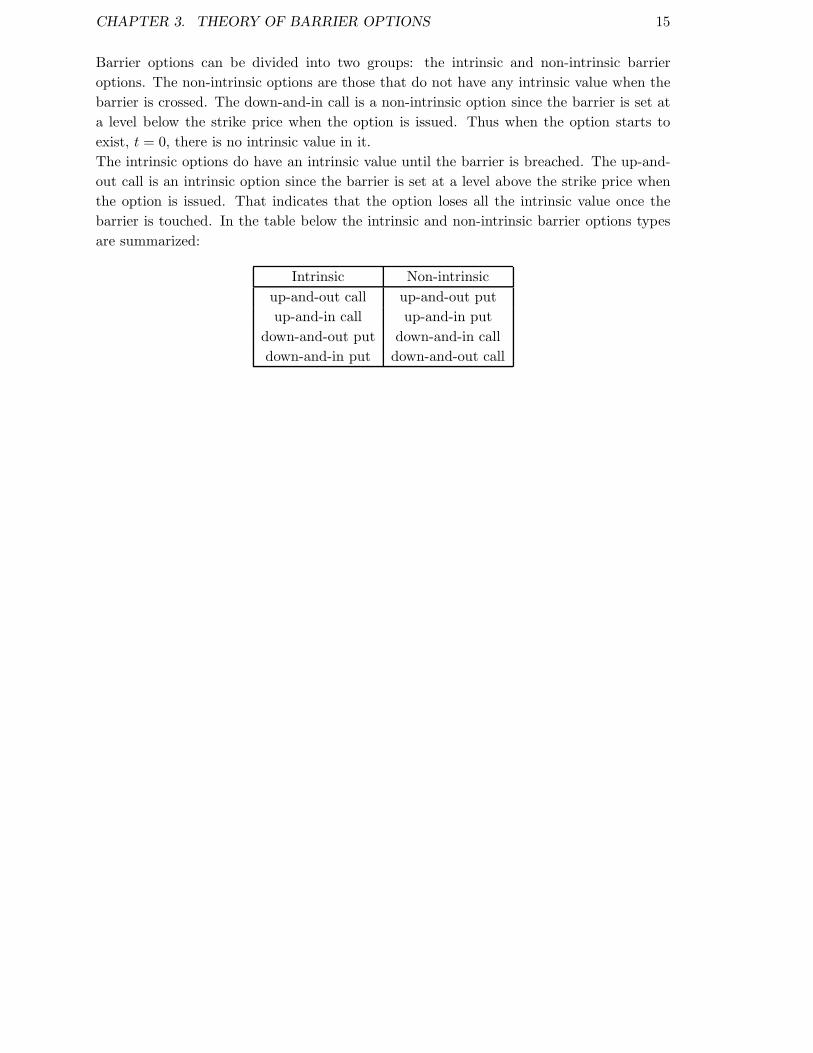
Barrier options can be divided into two groups: the intrinsic and non-intrinsic barrier
options. The non-intrinsic options are those that do not have any intrinsic value when the
barrier is crossed. The down-and-in call is a non-intrinsic option since the barrier is set at
a level below the strike price when the option is issued. Thus when the option starts to
exist, t = 0, there is no intrinsic value in it.
The intrinsic options do have an intrinsic value until the barrier is breached. The up-and-
out call is an intrinsic option since the barrier is set at a level above the strike price when
the option is issued. That indicates that the option loses all the intrinsic value once the
barrier is touched. In the table below the intrinsic and non-intrinsic barrier options types
are summarized:
Intrinsic Non-intrinsic
up-and-out call up-and-out put
up-and-in call up-and-in put
down-and-out put down-and-in call
down-and-in put down-and-out call
CHAPTER 3. THEORY OF BARRIER OPTIONS 16
3.2 Black-Scholes and barrier option pricing
(Merton 1973) proposed the first analytic formula for a down-and-out call option and later
(Reiner & Rubinstein 1991) provided the formulas for all four types of barrier on both call
and put options.
The price of a barrier option will depend on the standard Black-Scholes parameters, as well
as on the barrier level, B.
The outline in (Higham 2004, 197) is followed to derive the value of a Barrier Option. In
section 2.2.4 on page 11 showed a derivation of the Black-Schole partial differential equation
(PDE)∂V
∂t+
1
2σ2S2∂
2V
∂S2+ rS
∂V
∂S− rV = 0. (3.2)
Suppose that the function V (S, t) satisfies the Black-Scholes partial differential equation.
Set
V(S, t) = S1− 2r
σ2 V
(
B
S, t
)
. (3.3)
Thus
∂V
∂t= S1− 2r
σ2∂V
∂t
(
B
S, t
)
,
∂V
∂S=
(
1− 2r
σ2
)
S− 2r
σ2 V
(
B
S, t
)
−BS−1− 2r
σ2∂V
∂S
(
B
S, t
)
,
∂2V
∂S2=
(
1− 2r
σ2
)(−2r
σ2
)
S−1− 2r
σ2 V
(
B
S, t
)
+∂V
∂S
(
B
S, t
)(
4Br
σ2
)
S−2− 2r
σ2
+B2S−3− 2r
σ2∂2V
∂S2
(
B
S, t
)
.

CHAPTER 3. THEORY OF BARRIER OPTIONS 17
Substitute the above partial fraction expressions in (3.2). So,
∂V
∂t+
1
2σ2S2∂
2V
∂S2+ rS
∂V
∂S− rV
= S1− 2r
σ2∂V
∂t
(
B
S, t
)
−(
1− 2r
σ2
)
(r)S1− 2r
σ2 V
(
B
S, t
)
+2BrS− 2r
σ2∂V
∂S
(
B
S, t
)
+1
2σ2B2S−1− 2r
σ2∂2V
∂S2
(
B
S, t
)
+r
(
1− 2r
σ2
)
S1− 2r
σ2 V
(
B
S, t
)
− rBS− 2r
σ2∂V
∂S
(
B
S, t
)
−rS1− 2r
σ2 V
(
B
S, t
)
= S1− 2r
σ2∂V
∂t
(
B
S, t
)
+B2S−1− 2r
σ21
2σ2∂
2V
∂S2
(
B
S, t
)
+rBS− 2r
σ2∂V
∂S
(
B
S, t
)
−rV S1− 2r
σ2
(
B
S, t
)
= S1− 2r
σ2
[
∂V
∂t
(
B
S, t
)
+1
2σ2
(
B
S
)2 ∂2V
∂S2
(
B
S, t
)
+ rB
S
∂V
∂S
(
B
S, t
)
− rV
(
B
S, t
)
]
.
The term inside the block brackets is zero since V satisfies the Black-Scholes PDE. Thus V
solves the Black-Scholes PDE.
Similar to the derivation above, it can be proven that
cdown−in(S, t) =
(
S
B
)1− 2r
σ2
c
(
B2
S, T − t
)
,
solves the Black-Schole PDE, where c(
B2
S , T − t)
is calculated using equation (2.25).
One can then calculate the option value of a down-and-out call option, for K > B, on the

CHAPTER 3. THEORY OF BARRIER OPTIONS 18
domain 0 ≤ t ≤ T , B ≤ S by using the in-out parity.
c(S, t) = cdown−in(S, t) + cdown−out(S, t)
cdown−out(S, t) = c(S, t) − cdown−in(S, t)
= c(S, t) −(
S
B
)1− 2r
σ2
c
(
B2
S, T − t
)
.
An interesting observation
From equation above one can immediately observe that the down-and-out call is worth less
than the European call.
From section 2.2.4, equation (2.25) one finds
c(S, t) = SN
(
log(S/K) + (r + σ2/2)(T − t)
σ√T − t
)
−Ke−r(T−t)N
(
log(S/K) + (r − σ2/2)(T − t)
σ√T − t
)
,
where N(.) is the cumulative distribution function for a standardized normal random vari-
able given by
N(x) =1√2π
∫ x
−∞e−
1
2y2dy.
Thus
cdown−out(S, t) = c(S, t) − cdown−in(S, t)
= c(S, t) −(
S
B
)1− 2r
σ2
c
(
B2
S, T − t
)
= SN
(
log(S/K) + (r + σ2/2)(T − t)
σ√T − t
)
−Ke−r(T−t)N
(
log(S/K) + (r − σ2/2)(T − t)
σ√T − t
)
−B
(
S
B
−2rσ−2)
N
(
log(B2/SK) + (r + σ2/2)(T − t)
σ√T − t
)
−(
S
B
1−2rσ−2
Ke−r(T−t)
)
N
(
log(B2/SK) + (r − σ2/2)(T − t)
σ√T − t
)
.
Unless the barrier is crossed, the Black-Scholes partial differential equation (2.13) is ap-
plicable, thus cdown−out(S, t) must satisfy the partial differential equation on the domain
0 ≤ t ≤ T,B ≤ S, where
ct - European call option price(premium),
pt - European put option price (premium),

CHAPTER 3. THEORY OF BARRIER OPTIONS 19
St - Underlying asset’s price at time t,
K - Predetermined option strike price,
r - Risk-free interest rate,
σ - Volatility of the underlying.
When S(t∗) ≤ B for some t∗, then the option becomes worthless:
cdown−out(B, t) = 0, for t∗ ≤ t ≤ T.
At expiry, when S(t) > B for 0 ≤ t ≤ T , then one recovers the European value, so that:
cdown−out(S, t) = c(S, t), for B ≤ S,
where c(S, t) is from equation (2.25).
The method below will be referred to as the standard method :
According to (Wilmott 2007, 408), the continuously monitored barrier option values can be
calculated using the following formula mentioned below, where N(.) denotes the cumulative
distribution function for a standardized normal variable, B the barrier position, q the div-
idend yield , S the stock price and K the strike price. (Dewynne et al. 1995, 207) derives
the formulae below.
The following are formulae for the value of the call and put barrier options:
Consider a up-and-in and up-and-out call, with the barrier above the initial stock price
B > S0.
Up-and-out call:
1. K >B:
cup−out = 0.
If K > B then K > S0. According to (2.14) this means that the value of the option
will be 0.
2. K < B:
cup−out = Se−q(T−t)(N(d1)−N(d3)− b(N(d6)−N(d8)))−Ke−r(T−t)(N(d2)−N(d4)− a(N(d5)−N(d7))).
If K < B then one can have K ≤ S or K ≥ S and the value of the option is calculated
using the above formula.

CHAPTER 3. THEORY OF BARRIER OPTIONS 20
Up-and-in call:
1. K >B:
cup−in = 0.
If K > B then K > S0. According to (2.14) this means that the value of the option
will be 0.
2. K < B:
cup−in = Se−q(T−t)(N(d3) + b(N(d6)−N(d8))) −Ke−r(T−t)(N(d4) + a(N(d5)−N(d7)))).
If K < B then one can have K ≤ S or K ≥ S and the value of the option is calculated
using the above formula.
Consider a down-and-out and down-and-in put, with the barrier below the initial stock
price B < S0.
Down-and-out put:
1. K >B:
pdown−out = −Se−q(T−t)(N(d3)−N(d1)− b(N(d8)−N(d6))) +
Ke−r(T−t)(N(d4)−N(d2)− a(N(d7)−N(d5))).
If K > B then one can have K ≤ S or K ≥ S and the value of the option is calculated
using the above formula.
2. K < B:
pdown−out = 0.
If K < B then K < S0. According to (2.17) this means that the value of the option
will be 0.
Down-and-in put:
1. K >B:
pdown−in = −Se−q(T−t)(1−N(d3) + b(N(d8)−N(d6))) +
Ke−r(T−t)(1−N(d4) + a(N(d7)−N(d5))).
If K > B then one can have K ≤ S or K ≥ S and the value of the option is calculated
using the above formula.

CHAPTER 3. THEORY OF BARRIER OPTIONS 21
2. K < B:
pdown−in = 0.
If K < B then K < S0. According to (2.17) this means that the value of the option
will be 0.
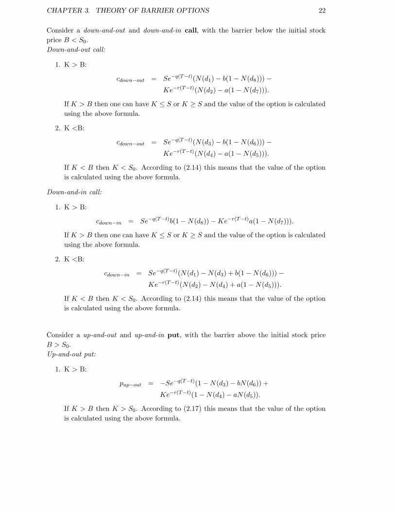
CHAPTER 3. THEORY OF BARRIER OPTIONS 22
Consider a down-and-out and down-and-in call, with the barrier below the initial stock
price B < S0.
Down-and-out call:
1. K > B:
cdown−out = Se−q(T−t)(N(d1)− b(1−N(d8))) −Ke−r(T−t)(N(d2)− a(1−N(d7))).
If K > B then one can have K ≤ S or K ≥ S and the value of the option is calculated
using the above formula.
2. K <B:
cdown−out = Se−q(T−t)(N(d3)− b(1−N(d6))) −Ke−r(T−t)(N(d4)− a(1−N(d5))).
If K < B then K < S0. According to (2.14) this means that the value of the option
is calculated using the above formula.
Down-and-in call:
1. K > B:
cdown−in = Se−q(T−t)b(1−N(d8))−Ke−r(T−t)a(1−N(d7))).
If K > B then one can have K ≤ S or K ≥ S and the value of the option is calculated
using the above formula.
2. K <B:
cdown−in = Se−q(T−t)(N(d1)−N(d3) + b(1−N(d6))) −Ke−r(T−t)(N(d2)−N(d4) + a(1−N(d5))).
If K < B then K < S0. According to (2.14) this means that the value of the option
is calculated using the above formula.
Consider a up-and-out and up-and-in put, with the barrier above the initial stock price
B > S0.
Up-and-out put:
1. K > B:
pup−out = −Se−q(T−t)(1−N(d3)− bN(d6)) +
Ke−r(T−t)(1−N(d4)− aN(d5)).
If K > B then K > S0. According to (2.17) this means that the value of the option
is calculated using the above formula.

CHAPTER 3. THEORY OF BARRIER OPTIONS 23
2. K <B:
pup−out = −Se−q(T−t)(1−N(d1)− bN(d8)) +
Ke−r(T−t)(1−N(d2)− aN(d7)).
If K < B then one can have K ≤ S or K ≥ S and the value of the option is calculated
using the above formula.
Up-and-in put:
1. K > B:
pup−in = −Se−q(T−t)(N(d3)−N(d1) + bN(d6)) +
Ke−r(T−t)(N(d4)−N(d2) + aN(d5)).
If K > B then K > S0. According to (2.17) this means that the value of the option
is calculated using the above formula.
2. K <B:
pup−in = −Se−q(T−t)bN(d8) +Ke−r(T−t)aN(d7).
If K < B then one can have K ≤ S or K ≥ S and the value of the option is calculated
using the above formula.
with
a =
(
B
S
)−1+2(r−q)/σ2
b =
(
B
S
)1+2(r−q)/σ2
d1 =log(S/K) + (r − q + 1
2σ2)(T − t)
σ√T − t
d2 =log(S/K) + (r − q − 1
2σ2)(T − t)
σ√T − t

CHAPTER 3. THEORY OF BARRIER OPTIONS 24
d3 =log(S/B) + (r − q + 1
2σ2)(T − t)
σ√T − t
d4 =log(S/B) + (r − q − 1
2σ2)(T − t)
σ√T − t
d5 =log(S/B)− (r − q − 1
2σ2)(T − t)
σ√T − t
d6 =log(S/B)− (r − q + 1
2σ2)(T − t)
σ√T − t
d7 =log(SK/B2)− (r − q − 1
2σ2)(T − t)
σ√T − t
d8 =log(SK/B2)− (r − q + 1
2σ2)(T − t)
σ√T − t
where ct - European call option price,
St - Underlying asset’s price at time t,
K - Predetermined option strike price,
r - Risk-free interest rate,
q - Dividend yield,
σ - Standard deviation.
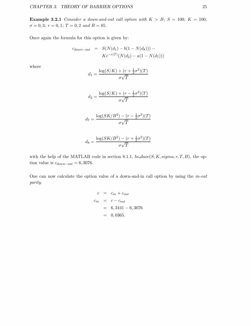
CHAPTER 3. THEORY OF BARRIER OPTIONS 25
Example 3.2.1 Consider a down-and-out call option with K > B; S = 100; K = 100;
σ = 0, 3; r = 0, 1; T = 0, 2 and B = 85.
Once again the formula for this option is given by:
cdown−out = S(N(d1)− b(1−N(d8)))−Ke−r(T )(N(d2)− a(1−N(d7)))
where
d1 =log(S/K) + (r + 1
2σ2)(T )
σ√T
d2 =log(S/K) + (r − 1
2σ2)(T )
σ√T
d7 =log(SK/B2)− (r − 1
2σ2)(T )
σ√T
d8 =log(SK/B2)− (r + 1
2σ2)(T )
σ√T
with the help of the MATLAB code in section 8.1.1, bs daoc(S,K, sigma, r, T,B), the op-
tion value is cdown−out = 6, 3076.
One can now calculate the option value of a down-and-in call option by using the in-out
parity.
c = cin + cout
cin = c− cout
= 6, 3441 − 6, 3076
= 0, 0365.
Chapter 4
Binomial and Trinomial Method
Analytical solutions do not always exist for real-world barrier options, either because the
barrier structure is complex or because it is discrete, (Derman et al. 1995). There are es-
sentially no analytical formulas for pricing discrete barrier options, and numerical pricing
is difficult and slow to converge, (Broadie et al. 1997). It is consequently necessary to in-
vestigate the efficiency of a number of numerical methods and adaptive methods.
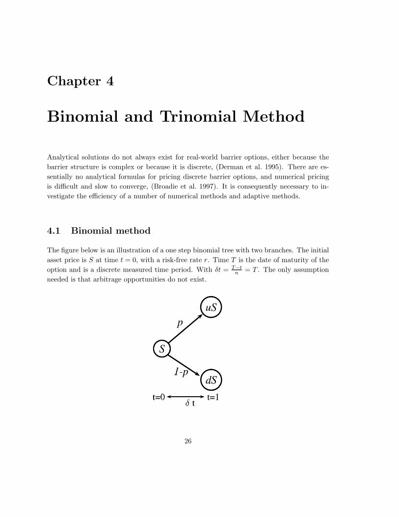
4.1 Binomial method
The figure below is an illustration of a one step binomial tree with two branches. The initial
asset price is S at time t = 0, with a risk-free rate r. Time T is the date of maturity of the
option and is a discrete measured time period. With δt = T−tn = T . The only assumption
needed is that arbitrage opportunities do not exist.
26
CHAPTER 4. BINOMIAL AND TRINOMIAL METHOD 27
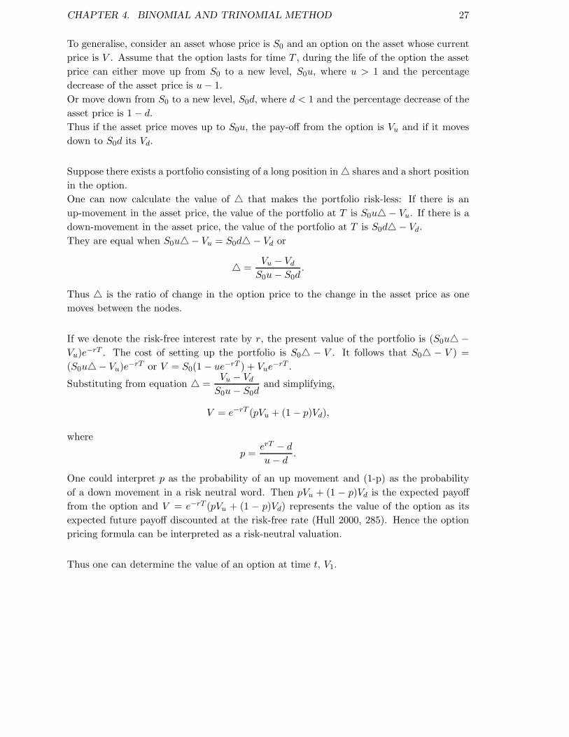
To generalise, consider an asset whose price is S0 and an option on the asset whose current
price is V . Assume that the option lasts for time T , during the life of the option the asset
price can either move up from S0 to a new level, S0u, where u > 1 and the percentage
decrease of the asset price is u− 1.
Or move down from S0 to a new level, S0d, where d < 1 and the percentage decrease of the
asset price is 1− d.
Thus if the asset price moves up to S0u, the pay-off from the option is Vu and if it moves
down to S0d its Vd.
Suppose there exists a portfolio consisting of a long position in △ shares and a short position
in the option.
One can now calculate the value of △ that makes the portfolio risk-less: If there is an
up-movement in the asset price, the value of the portfolio at T is S0u△− Vu. If there is a
down-movement in the asset price, the value of the portfolio at T is S0d△− Vd.
They are equal when S0u△− Vu = S0d△− Vd or
△ =Vu − Vd
S0u− S0d.
Thus △ is the ratio of change in the option price to the change in the asset price as one
moves between the nodes.
If we denote the risk-free interest rate by r, the present value of the portfolio is (S0u△−Vu)e
−rT . The cost of setting up the portfolio is S0△ − V . It follows that S0△ − V ) =
(S0u△− Vu)e−rT or V = S0(1− ue−rT ) + Vue
−rT .
Substituting from equation △ =Vu − Vd
S0u− S0dand simplifying,
V = e−rT (pVu + (1− p)Vd),
where
p =erT − d
u− d.
One could interpret p as the probability of an up movement and (1-p) as the probability
of a down movement in a risk neutral word. Then pVu + (1 − p)Vd is the expected payoff
from the option and V = e−rT (pVu + (1 − p)Vd) represents the value of the option as its
expected future payoff discounted at the risk-free rate (Hull 2000, 285). Hence the option
pricing formula can be interpreted as a risk-neutral valuation.
Thus one can determine the value of an option at time t, V1.

CHAPTER 4. BINOMIAL AND TRINOMIAL METHOD 28
For one time step,
V1 = e−rδt((p)V u2 + (1− p)V d
2 )
where
V u2 = max(uS −K, 0), (4.1)
V d2 = max(dS −K, 0) (4.2)
and K = strike price.
To generalize one can determine the value of an option at time t, Vt, as
Vt = e−rδt(pV ut+δt + (1− p)V d
t+δt) (4.3)
where V ut+δt is the value of the option at time t+ δt if the value of the asset increases, and
V dt+δt is its value if the asset price decreases.
Thus, in order to price an option, one divides the period of the contract [0, T ] into a certain
number of subintervals, with a binomial process occurring in each time interval. One then
uses the payoff equation (2.14) or (2.17) at the end of the interval [t = T ].
Then one uses equation (4.3) to move backwards in time through the tree. Since risk neu-
trality is assumed, the value at each node at time T − δt can be calculated as the expected
value at time T discounted at rate r for a time period δt. In the same way, the value at
each node at time T −2δt can be calculated as the expected value at time T − δt discounted
for a time period δt at rate r, and so on until one reaches a price at the beginning of the
interval, which is the value of the option (Hull 2000, 390).
CHAPTER 4. BINOMIAL AND TRINOMIAL METHOD 29
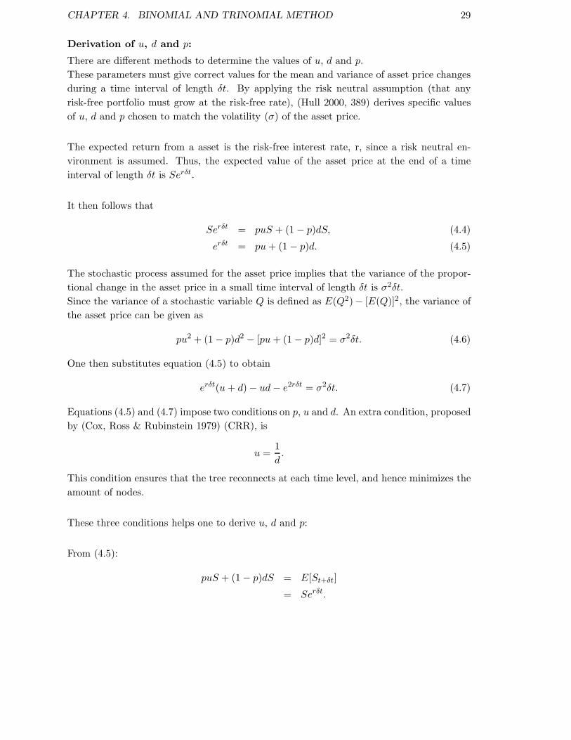
Derivation of u, d and p:
There are different methods to determine the values of u, d and p.
These parameters must give correct values for the mean and variance of asset price changes
during a time interval of length δt. By applying the risk neutral assumption (that any
risk-free portfolio must grow at the risk-free rate), (Hull 2000, 389) derives specific values
of u, d and p chosen to match the volatility (σ) of the asset price.
The expected return from a asset is the risk-free interest rate, r, since a risk neutral en-
vironment is assumed. Thus, the expected value of the asset price at the end of a time
interval of length δt is Serδt.
It then follows that
Serδt = puS + (1− p)dS, (4.4)
erδt = pu+ (1− p)d. (4.5)
The stochastic process assumed for the asset price implies that the variance of the propor-
tional change in the asset price in a small time interval of length δt is σ2δt.
Since the variance of a stochastic variable Q is defined as E(Q2)− [E(Q)]2, the variance of
the asset price can be given as
pu2 + (1− p)d2 − [pu+ (1− p)d]2 = σ2δt. (4.6)
One then substitutes equation (4.5) to obtain
erδt(u+ d)− ud− e2rδt = σ2δt. (4.7)
Equations (4.5) and (4.7) impose two conditions on p, u and d. An extra condition, proposed
by (Cox, Ross & Rubinstein 1979) (CRR), is
u =1
d.
This condition ensures that the tree reconnects at each time level, and hence minimizes the
amount of nodes.
These three conditions helps one to derive u, d and p:
From (4.5):
puS + (1− p)dS = E[St+δt]
= Serδt.

CHAPTER 4. BINOMIAL AND TRINOMIAL METHOD 30
One divides by S
pu+ (1− p)d = erδt
pu+ d− pd = erδt
p(u− d) = erδt − d.
Thus
p =erδt − d
u− d, (4.8)
var(St+δt) = E[S2t+δt]− E[St+δt]
2.
Thus from the variance equation (4.6):
σ2δt = pu2 + (1− p)d2 − [pu+ (1− p)d]2
= pu2 + (1− p)d2 − p2u2 − 2p(1− p)ud− (1− p)2d2
= u2(p− p2) + [(1− p)− (1− p)2]d2 − 2p(1− p)ud
= u2p(1− p) + (1− p)[1− (1− p)]d2 − 2p(1− p)ud
= u2p(1− p) + (1− p)(p)d2 − 2p(1− p)ud
= p(1− p)[u2 − 2ud+ d2].
Hence
σ2δt = p(1− p)(u− d)2. (4.9)
Using (4.8) one obtains
p(1− p) = p− p2
=erδt − d
u− d− e2rδt − 2derδt + d2
(u− d)2
=erδtu− ud− erδtd+ d2 − e2rδt + 2derδt − d2
(u− d)2
=erδt(u− d+ 2d)− ud− e2rδt
(u− d)2
=erδt(u+ d)− ud− e2rδt
(u− d)2.
Hence
p(1− p) =erδt(u+ d)− ud− e2rδt
(u− d)2. (4.10)
CHAPTER 4. BINOMIAL AND TRINOMIAL METHOD 31
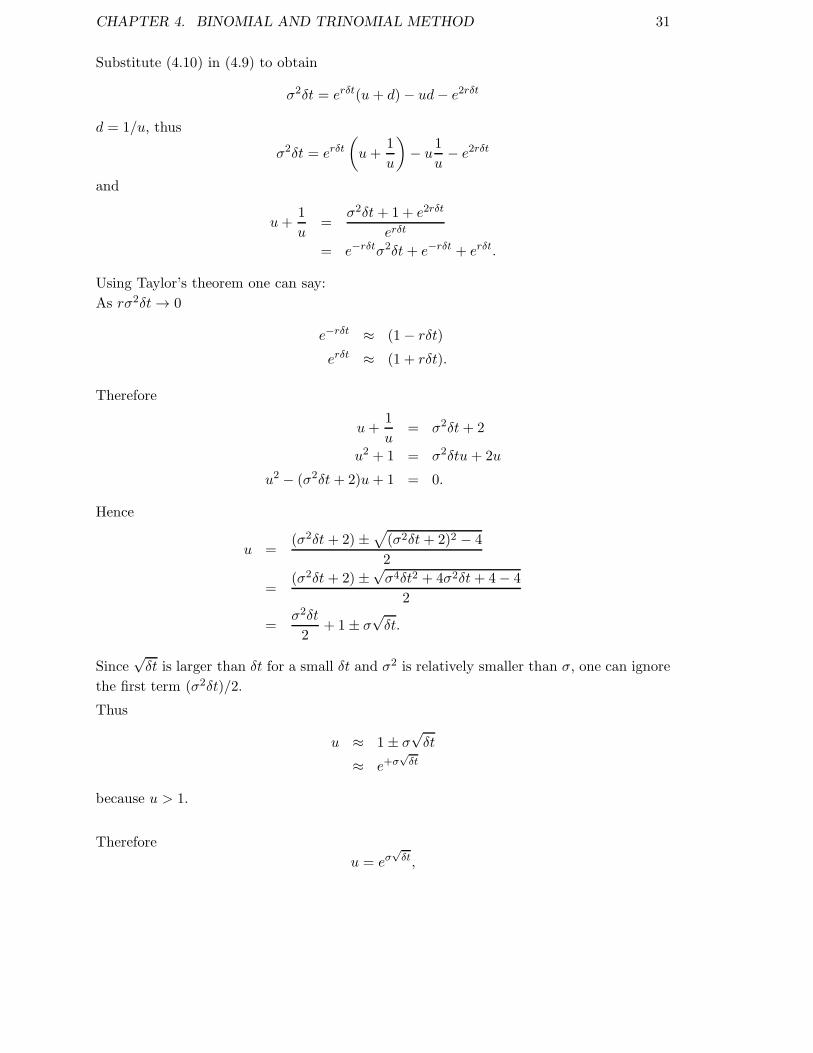
Substitute (4.10) in (4.9) to obtain
σ2δt = erδt(u+ d)− ud− e2rδt
d = 1/u, thus
σ2δt = erδt(
u+1
u
)
− u1
u− e2rδt
and
u+1
u=
σ2δt+ 1 + e2rδt
erδt
= e−rδtσ2δt+ e−rδt + erδt.
Using Taylor’s theorem one can say:
As rσ2δt → 0
e−rδt ≈ (1− rδt)
erδt ≈ (1 + rδt).
Therefore
u+1
u= σ2δt+ 2
u2 + 1 = σ2δtu+ 2u
u2 − (σ2δt+ 2)u+ 1 = 0.
Hence
u =(σ2δt+ 2)±
√
(σ2δt+ 2)2 − 4
2
=(σ2δt+ 2)±
√σ4δt2 + 4σ2δt+ 4− 4
2
=σ2δt
2+ 1± σ
√δt.
Since√δt is larger than δt for a small δt and σ2 is relatively smaller than σ, one can ignore
the first term (σ2δt)/2.
Thus
u ≈ 1± σ√δt
≈ e+σ√δt
because u > 1.
Therefore
u = eσ√δt,

CHAPTER 4. BINOMIAL AND TRINOMIAL METHOD 32
d = e−σ√δt
and
p =erδt − d
u− d.
�
(Higham 2004, 153) chooses p = 0, 5 and then obtains
u = eσ√δt+(r− 1
2σ2)δt
and
d = e−σ√δt+(r− 1
2σ2)δt.
Standard binomial method algorithm
Assume there are two time steps (N) and that S0 is the initial asset price.
1. First work out the value of the asset at every node.
Thus, at t = 0
Sn1 = S0.
CHAPTER 4. BINOMIAL AND TRINOMIAL METHOD 33
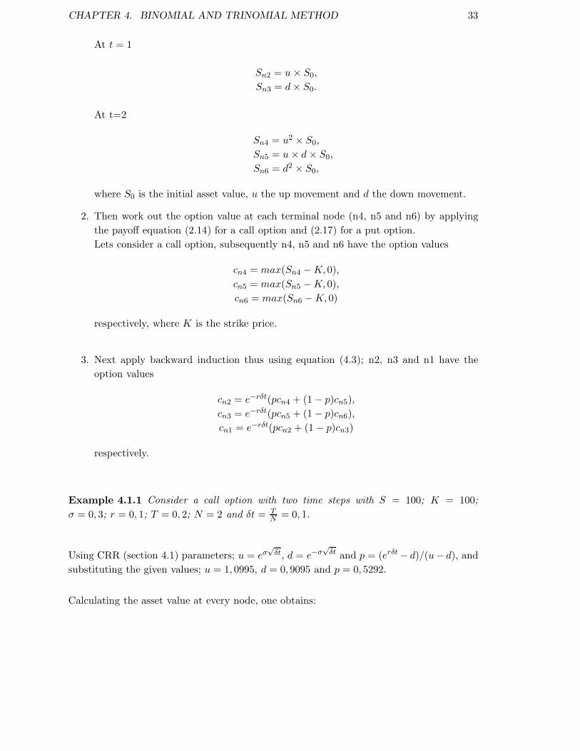
At t = 1
Sn2 = u× S0,
Sn3 = d× S0.
At t=2
Sn4 = u2 × S0,
Sn5 = u× d× S0,
Sn6 = d2 × S0,
where S0 is the initial asset value, u the up movement and d the down movement.
2. Then work out the option value at each terminal node (n4, n5 and n6) by applying
the payoff equation (2.14) for a call option and (2.17) for a put option.
Lets consider a call option, subsequently n4, n5 and n6 have the option values
cn4 = max(Sn4 −K, 0),
cn5 = max(Sn5 −K, 0),
cn6 = max(Sn6 −K, 0)
respectively, where K is the strike price.
3. Next apply backward induction thus using equation (4.3); n2, n3 and n1 have the
option values
cn2 = e−rδt(pcn4 + (1− p)cn5),
cn3 = e−rδt(pcn5 + (1− p)cn6),
cn1 = e−rδt(pcn2 + (1− p)cn3)
respectively.
Example 4.1.1 Consider a call option with two time steps with S = 100; K = 100;
σ = 0, 3; r = 0, 1; T = 0, 2; N = 2 and δt = TN = 0, 1.
Using CRR (section 4.1) parameters; u = eσ√δt, d = e−σ
√δt and p = (erδt − d)/(u− d), and
substituting the given values; u = 1, 0995, d = 0, 9095 and p = 0, 5292.
Calculating the asset value at every node, one obtains:

CHAPTER 4. BINOMIAL AND TRINOMIAL METHOD 34
Then calculate the option value at each terminal node by using the payoff equation c(S, t) =
max(S −K, 0). Nodes n4, n5 and n6 option values are then
cn4 = 20, 89;
cn5 = 0;
cn6 = 0
respectively.
(For example: cn4 = max(120, 89 − 100; 0) = 20, 89)
Then apply backward induction to get the options values of nodes n2, n3 and finally n1.
Using the equations
cn2 = e−rδt(pcn4 + (1− p)cn5),
cn3 = e−rδt(pcn5 + (1− p)cn6),
cn1 = e−rδt(pcn2 + (1− p)cn3)
and substitute the valid numerical data.
(For example: cn2 = e−0.1×0.1(0, 5292 × 20, 89 + (1− 0, 5292) × 0) = 10, 94)
One can then obtain the option value at each node:
CHAPTER 4. BINOMIAL AND TRINOMIAL METHOD 35
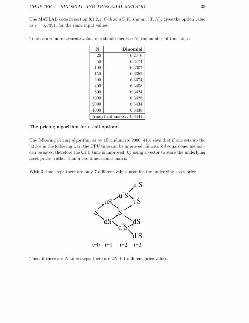
The MATLAB code in section 8.1.2.1, Call bm(S,K, sigma, r, T,N), gives the option value
as c = 5, 7351, for the same input values.
To obtain a more accurate value, one should increase N , the number of time steps.
N Binomial
20 6,2776
50 6,3174
100 6,3307
150 6,3352
200 6,3374
400 6,3408
800 6,3424
1000 6,3428
2000 6,3434
4000 6,3438
Analytical answer: 6,3441
The pricing algorithm for a call option:
The following pricing algorithm as by (Brandimarte 2006, 413) says that if one sets up the
lattice in the following way, the CPU time can be improved. Since u×d equals one, memory
can be saved therefore the CPU time is improved, by using a vector to store the underlying
asset prices, rather than a two-dimensional matrix.
With 3 time steps there are only 7 different values used for the underlying asset price.
Thus, if there are N time steps, there are 2N + 1 different price values.

CHAPTER 4. BINOMIAL AND TRINOMIAL METHOD 36
The numbers shown in the picture above are locations in the vector. Thus in element 1 the
lowest value is stored resulting from a sequence of down steps only (dS). Note that you
obtain the same values in different locations in the tree (i.e. at t=0 and t=2 the location
indicated by 4 will have the same value).
Even-numbered entries correspond to the second-to-last time layer and odd-numbered en-
tries correspond to the last time layer. Depending on the number of time steps, the number
of branches of the lattice may be even or odd-numbered.
Brandimarte uses this pattern to store option values in his program, thus using one vector
of 2N + 1 elements elements instead of using huge matrix’s that take a lot of memory (i.e.
in the picture above, 7 storage places are used instead of 10 individual storage places). Note
that as the number of time steps increase so will the storage places, making Brandimarte’s
program efficient. Below is steps explaining how the program is complied to give the final
option price.
1. First precompute invariant quantities, including the discounted probabilities, in the
first section of the code.
2. Then write the vector S(i) of underlying asset prices, start with the smallest element,
which is SdN . Next multiply by u, storing S0 in element S(N + 1), which is the
mid-element, and then proceed both up and down.
3. When one works with call values c(i), the index steps over by two, which amounts to
alternating odd- and even-indexed values corresponding to consecutive time layers.
4. When time to maturity is τ , one needs to consider only the 2(N − τ) + 1 innermost
elements of the array c(i). The option price is stored in the root of the lattice, which
corresponds to position N + 1 (Brandimarte 2006, 412).
set the initial option value S(1) = SdN
set the rest of the Option values:

CHAPTER 4. BINOMIAL AND TRINOMIAL METHOD 37
for i = 2 to 2N + 1
compute: S(i) = uS(i− 1)
end
set the terminal call values:
for i = 1 to 2 to 2N + 1
compute: c(i)=maximum(S(i) - K,0)
end
Work backwards to set the rest of the call values
for tau equal 1 to N
for i equal (tau+ 1) to 2 to (2N + 1− tau)
compute: c(i) = e−rδt(pc(i+ 1) + (1− p)(c(i − 1)))
end
end
Final call value = c(N+1)
where
c - European call option price,
S - Underlying asset’s price,
K - Predetermined option strike price,
r - Risk-free interest rate,
σ - Standard deviation,
p - Probability of upward or downward movement,
u - upward movement factor,
d - downward movement factor,
t - time to maturity,
δt - length of time interval,
N - number of time steps.
In section 8.1.2.1, the program Call bm is based on the above described algorithm.

CHAPTER 4. BINOMIAL AND TRINOMIAL METHOD 38
4.1.1 Accuracy of option value
In real world financial problems, the number of time steps (N) are not a known factor. Thus,
to find the option value accurately, it is important to have a program that can efficiently
calculate N . A proficient way of doing this is by modifying the previous method, by adding
a tolerance(tol).
The resulting algorithm can be summarized as follows:
set Option value old = 0
for N=1 to 5000
compute: Option value new = binomial method option value
if |Option value new- Option value old| < tolerance
break (stop)
end
set Option value old= Option value new
end
Example 4.1.2 Consider a call option with S = 100; K = 100; σ = 0, 3; r = 0, 1 and
T = 0, 2.
With the help of the MATLAB code found in section 8.1.2.2, newtest bm(S,K, sigma, r, T, tol),
one obtains the following table:
N Tol c
262 0,01 6,3390
2615 0,001 6,3446
Analytical answer: 6,3441
On an intel core i5 processor pc, when the tol = 0, 01 it took 0, 042 seconds and when the
tol = 0, 001 it took 30, 338 seconds.
According to Black-Scholes the analytic solution for the call option is 6, 3441.

CHAPTER 4. BINOMIAL AND TRINOMIAL METHOD 39
4.2 Trinomial method
Trinomial trees provide an effective method of numerical calculation of option prices within
Black-Scholes share pricing model. Trinomial trees can be used as an alternative to bino-
mial trees.
(Ritchken 1995) notes that the trinomial trees have a distinct advantage over binomial trees.
The asset price can move in three directions from a given node, thus the number of time
steps can be reduced and one can still attain the same accuracy as in the binomial tree.
The trinomial tree offers more flexibility than the binomial tree and is therefore useful when
pricing complex derivatives.
To discretize a geometric Brownian motion, the jump sizes and probabilities must match
the mean and variance. A possible choice to determine the jump sizes, is to build a trino-
mial tree where the asset price at each node can go up, stay at the same level, or go down
(Haug 1998, 300).
The parameters pu, pd and pm that are considered in this chapter are derived in (Haug 1998,
300).
There are different methods to determine these parameters, such as in (Haug 1998, 300):
u = eσ√2δt,
d = e−σ√2δt,
pu =
(
erδt/2 − e−σ√
δt/2
eσ√
δt/2 − e−σ√
δt/2
)2
,
CHAPTER 4. BINOMIAL AND TRINOMIAL METHOD 40
pd =
(
eσ√
δt/2 − erδt/2
eσ√
δt/2 − e−σ√
δt/2
)2
,
pm = 1− pu − pd,
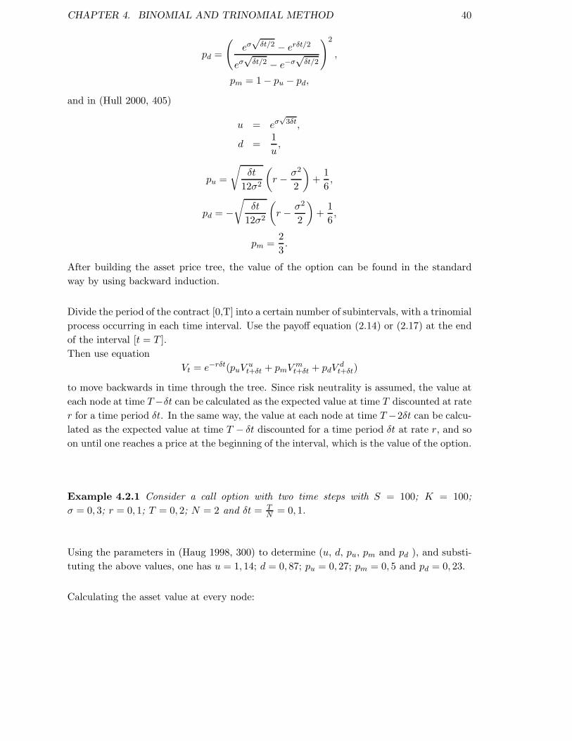
and in (Hull 2000, 405)
u = eσ√3δt,
d =1
u,
pu =
√
δt
12σ2
(
r − σ2
2
)
+1
6,
pd = −√
δt
12σ2
(
r − σ2
2
)
+1
6,
pm =2
3.
After building the asset price tree, the value of the option can be found in the standard
way by using backward induction.
Divide the period of the contract [0,T] into a certain number of subintervals, with a trinomial
process occurring in each time interval. Use the payoff equation (2.14) or (2.17) at the end
of the interval [t = T ].
Then use equation
Vt = e−rδt(puVut+δt + pmV m
t+δt + pdVdt+δt)
to move backwards in time through the tree. Since risk neutrality is assumed, the value at
each node at time T−δt can be calculated as the expected value at time T discounted at rate
r for a time period δt. In the same way, the value at each node at time T −2δt can be calcu-
lated as the expected value at time T − δt discounted for a time period δt at rate r, and so
on until one reaches a price at the beginning of the interval, which is the value of the option.
Example 4.2.1 Consider a call option with two time steps with S = 100; K = 100;
σ = 0, 3; r = 0, 1; T = 0, 2; N = 2 and δt = TN = 0, 1.
Using the parameters in (Haug 1998, 300) to determine (u, d, pu, pm and pd ), and substi-
tuting the above values, one has u = 1, 14; d = 0, 87; pu = 0, 27; pm = 0, 5 and pd = 0, 23.
Calculating the asset value at every node:

CHAPTER 4. BINOMIAL AND TRINOMIAL METHOD 41
Calculate the option value at each terminal node by using the equation c(S, t) = max(S −K, 0), where K = strike price.
Nodes n5, n6, n7, n8 and n9 option values are then
cn5 = 30, 78;
cn6 = 14, 36;
cn7 = 0;
cn8 = 0;
cn9 = 0
respectively.
(For example: c4 = max(130, 78 − 100; 0) = 30, 78 ).
Then apply backward induction and get the options values using the equations
cn2 = e−rδt(pucn5 + pmcn6 + pdcn7),
cn3 = e−rδt(pucn6 + pmcn7 + pdcn8),
cn4 = e−rδt(pucn7 + pmcn8 + pdcn9),
cn1 = e−rδt(pucn2 + pmcn3 + pdcn4),
and substitute the valid numerical data.
(For example: cn2 = e−0,1×0,1(0, 27 × 30, 78 + 0, 5 × 14, 36 + 0, 23 × 0) = 15, 35).
Obtain the option value at each node:

CHAPTER 4. BINOMIAL AND TRINOMIAL METHOD 42
The MATLAB code found in section 8.1.2.3, Call tm(S,K, sigma, r, T,N), using the same
input values gives the option value as c = 6, 0229, which is similar to the hand worked out
example above.
To obtain a more accurate value, one should increase N .
N Trinomial
20 6,3108
50 6,3307
100 6,3374
150 6,3397
200 6,3408
400 6,3424
800 6,3433
1000 6,3434
2000 6,3438
4000 6,3439
Analytical answer: 6,3441
CHAPTER 4. BINOMIAL AND TRINOMIAL METHOD 43
4.3 Barrier options for the binomial and trinomial method
The procedures for pricing knock-out and knock-in options through binomial/trinomial tree
methods work on exactly the same principal as standard options and the pricing method
is a two-step procedure. First value the options at every point above (up) or below (out)
the barrier. With the knock-out options, values below the barrier are equal to the value
of the rebate, unless there is no rebate, then the barrier values are equal to zero. Whereas
with the knock-in options, barrier values are equal to the value of an ordinary put or call
settled when the spot price breaches the barrier. Once the values are determined along the
barrier, use the payoff equation at the remaining terminal [t = T ] nodes and then perform
backward induction. The technique is similar to what is done with ordinary puts and calls,
except one works backwards from every point along the barrier, not just from the terminal
nodes (Chriss 1997, 452).
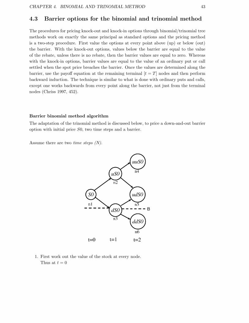
Barrier binomial method algorithm
The adaptation of the trinomial method is discussed below, to price a down-and-out barrier
option with initial price S0, two time steps and a barrier.
Assume there are two time steps (N).
1. First work out the value of the stock at every node.
Thus at t = 0
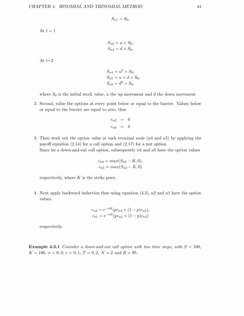
CHAPTER 4. BINOMIAL AND TRINOMIAL METHOD 44
Sn1 = S0.
At t = 1
Sn2 = u× S0,
Sn3 = d× S0.
At t=2
Sn4 = u2 × S0,
Sn5 = u× d× S0,
Sn6 = d2 × S0,
where S0 is the initial stock value, u the up movement and d the down movement.
2. Second, value the options at every point below or equal to the barrier. Values below
or equal to the barrier are equal to zero, thus
cn3 = 0
cn6 = 0
3. Then work out the option value at each terminal node (n4 and n5) by applying the
payoff equation (2.14) for a call option and (2.17) for a put option.
Since its a down-and-out call option, subsequently n4 and n5 have the option values
cn4 = max(Sn4 −K, 0),
cn5 = max(Sn5 −K, 0)
respectively, where K is the strike price.
4. Next apply backward induction thus using equation (4.3), n2 and n1 have the option
values
cn2 = e−rδt(pcn4 + (1− p)cn5),
cn1 = e−rδt(pcn2 + (1− p)cn3)
respectively.
Example 4.3.1 Consider a down-and-out call option with two time steps, with S = 100,
K = 100, σ = 0, 3; r = 0, 1; T = 0, 2; N = 2 and B = 95.
CHAPTER 4. BINOMIAL AND TRINOMIAL METHOD 45
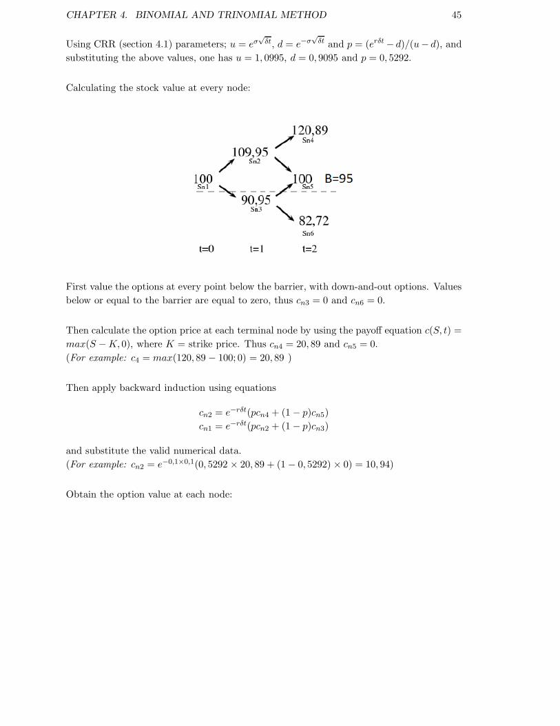
Using CRR (section 4.1) parameters; u = eσ√δt, d = e−σ
√δt and p = (erδt − d)/(u− d), and
substituting the above values, one has u = 1, 0995, d = 0, 9095 and p = 0, 5292.
Calculating the stock value at every node:
First value the options at every point below the barrier, with down-and-out options. Values
below or equal to the barrier are equal to zero, thus cn3 = 0 and cn6 = 0.
Then calculate the option price at each terminal node by using the payoff equation c(S, t) =
max(S −K, 0), where K = strike price. Thus cn4 = 20, 89 and cn5 = 0.
(For example: c4 = max(120, 89 − 100; 0) = 20, 89 )
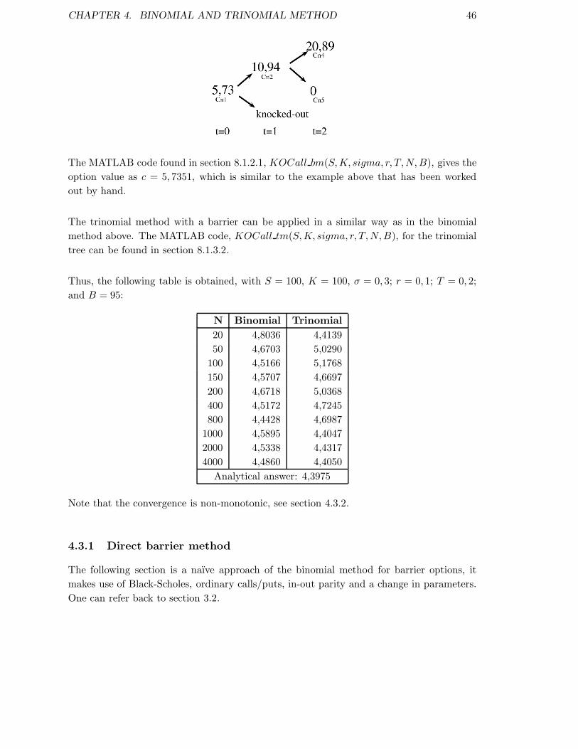
Then apply backward induction using equations
cn2 = e−rδt(pcn4 + (1− p)cn5)
cn1 = e−rδt(pcn2 + (1− p)cn3)
and substitute the valid numerical data.
(For example: cn2 = e−0,1×0,1(0, 5292 × 20, 89 + (1− 0, 5292) × 0) = 10, 94)
Obtain the option value at each node:
CHAPTER 4. BINOMIAL AND TRINOMIAL METHOD 46
The MATLAB code found in section 8.1.2.1, KOCall bm(S,K, sigma, r, T,N,B), gives the
option value as c = 5, 7351, which is similar to the example above that has been worked
out by hand.
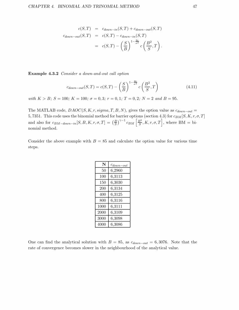
The trinomial method with a barrier can be applied in a similar way as in the binomial
method above. The MATLAB code, KOCall tm(S,K, sigma, r, T,N,B), for the trinomial
tree can be found in section 8.1.3.2.
Thus, the following table is obtained, with S = 100, K = 100, σ = 0, 3; r = 0, 1; T = 0, 2;
and B = 95:
N Binomial Trinomial
20 4,8036 4,4139
50 4,6703 5,0290
100 4,5166 5,1768
150 4,5707 4,6697
200 4,6718 5,0368
400 4,5172 4,7245
800 4,4428 4,6987
1000 4,5895 4,4047
2000 4,5338 4,4317
4000 4,4860 4,4050
Analytical answer: 4,3975
Note that the convergence is non-monotonic, see section 4.3.2.
4.3.1 Direct barrier method
The following section is a naıve approach of the binomial method for barrier options, it
makes use of Black-Scholes, ordinary calls/puts, in-out parity and a change in parameters.
One can refer back to section 3.2.
CHAPTER 4. BINOMIAL AND TRINOMIAL METHOD 47
c(S, T ) = cdown−in(S, T ) + cdown−out(S, T )
cdown−out(S, T ) = c(S, T )− cdown−in(S, T )
= c(S, T )−(
S
B
)1− 2r
σ2
c
(
B2
S, T
)
.
Example 4.3.2 Consider a down-and-out call option
cdown−out(S, T ) = c(S, T )−(
S
B
)1− 2r
σ2
c
(
B2
S, T
)
(4.11)
with K > B; S = 100; K = 100; σ = 0, 3; r = 0, 1; T = 0, 2; N = 2 and B = 95.
The MATLAB code, DAOC(S,K, r, sigma, T,B,N), gives the option value as cdown−out =
5, 7351. This code uses the binomial method for barrier options (section 4.3) for cBM [S,K, r, σ, T ]
and also for cBM−down−in[S,B,K, r, σ, T ] =(
BS
)γ−1cBM
[
B2
S ,K, r, σ, T]
, where BM = bi-
nomial method.
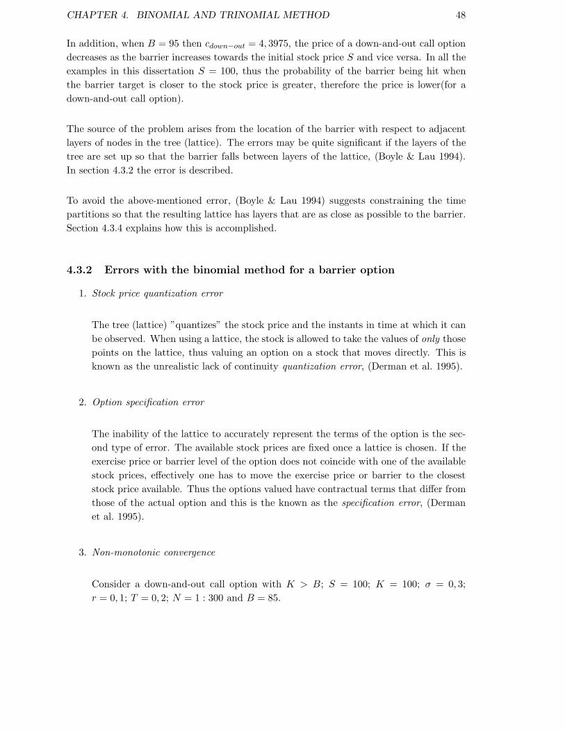
Consider the above example with B = 85 and calculate the option value for various time
steps.
N cdown−out
50 6,2960
100 6,3113
150 6,3030
200 6,3134
400 6,3125
800 6,3116
1000 6,3111
2000 6,3109
3000 6,3098
4000 6,3086
One can find the analytical solution with B = 85, as cdown−out = 6, 3076. Note that the
rate of convergence becomes slower in the neighbourhood of the analytical value.
CHAPTER 4. BINOMIAL AND TRINOMIAL METHOD 48
In addition, when B = 95 then cdown−out = 4, 3975, the price of a down-and-out call option
decreases as the barrier increases towards the initial stock price S and vice versa. In all the
examples in this dissertation S = 100, thus the probability of the barrier being hit when
the barrier target is closer to the stock price is greater, therefore the price is lower(for a
down-and-out call option).
The source of the problem arises from the location of the barrier with respect to adjacent
layers of nodes in the tree (lattice). The errors may be quite significant if the layers of the
tree are set up so that the barrier falls between layers of the lattice, (Boyle & Lau 1994).
In section 4.3.2 the error is described.
To avoid the above-mentioned error, (Boyle & Lau 1994) suggests constraining the time
partitions so that the resulting lattice has layers that are as close as possible to the barrier.
Section 4.3.4 explains how this is accomplished.
4.3.2 Errors with the binomial method for a barrier option
1. Stock price quantization error
The tree (lattice) ”quantizes” the stock price and the instants in time at which it can
be observed. When using a lattice, the stock is allowed to take the values of only those
points on the lattice, thus valuing an option on a stock that moves directly. This is
known as the unrealistic lack of continuity quantization error, (Derman et al. 1995).
2. Option specification error
The inability of the lattice to accurately represent the terms of the option is the sec-
ond type of error. The available stock prices are fixed once a lattice is chosen. If the
exercise price or barrier level of the option does not coincide with one of the available
stock prices, effectively one has to move the exercise price or barrier to the closest
stock price available. Thus the options valued have contractual terms that differ from
those of the actual option and this is the known as the specification error, (Derman
et al. 1995).
3. Non-monotonic convergence
Consider a down-and-out call option with K > B; S = 100; K = 100; σ = 0, 3;
r = 0, 1; T = 0, 2; N = 1 : 300 and B = 85.
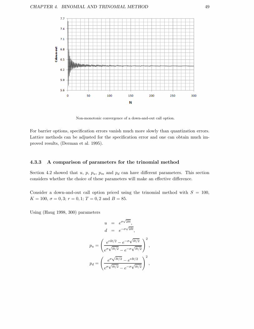
CHAPTER 4. BINOMIAL AND TRINOMIAL METHOD 49
Non-monotonic convergence of a down-and-out call option.
For barrier options, specification errors vanish much more slowly than quantization errors.
Lattice methods can be adjusted for the specification error and one can obtain much im-
proved results, (Derman et al. 1995).
4.3.3 A comparison of parameters for the trinomial method
Section 4.2 showed that u, p, pu, pm and pd can have different parameters. This section
considers whether the choice of these parameters will make an effective difference.
Consider a down-and-out call option priced using the trinomial method with S = 100,
K = 100, σ = 0, 3; r = 0, 1; T = 0, 2 and B = 85.
Using (Haug 1998, 300) parameters
u = eσ√2δt,
d = e−σ√2δt,
pu =
(
erδt/2 − e−σ√
δt/2
eσ√
δt/2 − e−σ√
δt/2
)2
,
pd =
(
eσ√
δt/2 − erδt/2
eσ√
δt/2 − e−σ√
δt/2
)2
,

CHAPTER 4. BINOMIAL AND TRINOMIAL METHOD 50
pm = 1− pu − pd,
and (Hull 2000, 405) parameters
u = eσ√3δt,
d =1
u,
pu =
√
δt
12σ2
(
r − σ2
2
)
+1
6,
pd = −√
δt
12σ2
(
r − σ2
2
)
+1
6,
pm =2
3,
the following results are obtained:
N Haug Hull
20 6,2890 6,2736
50 6,3209 6,2851
100 6,3134 6,2952
150 6,3149 6,3106
200 6,3202 6,3041
400 6,3177 6,3047
800 6,3146 6,3089
1000 6,3152 6,3158
2000 6,3119 6,3127
3000 6,3079 6,3118
4000 6,3114 6,3117
5000 6,3093 6,3102
The analytical down-and-out call option price to this example is 6, 3076. Thus the param-
eters make little difference, a large number of time steps are required for both to obtain an
accurate answer. Also note that the convergence is not monotonic.
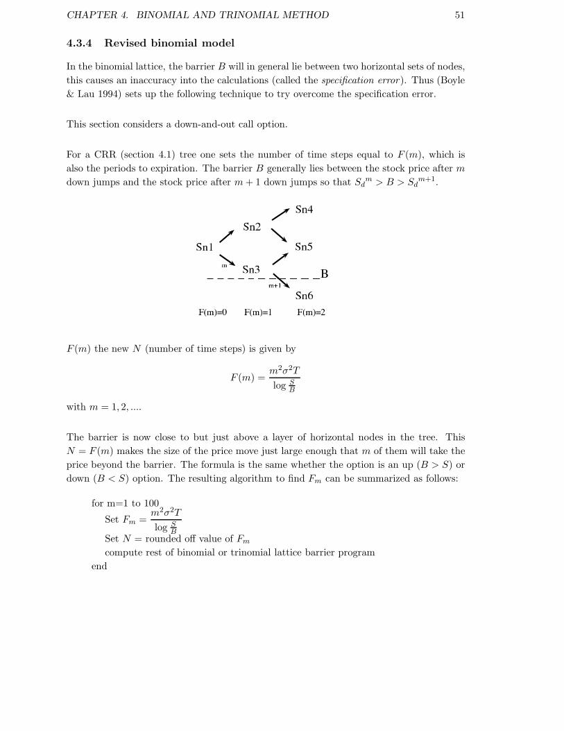
CHAPTER 4. BINOMIAL AND TRINOMIAL METHOD 51
4.3.4 Revised binomial model
In the binomial lattice, the barrier B will in general lie between two horizontal sets of nodes,
this causes an inaccuracy into the calculations (called the specification error). Thus (Boyle
& Lau 1994) sets up the following technique to try overcome the specification error.
This section considers a down-and-out call option.
For a CRR (section 4.1) tree one sets the number of time steps equal to F (m), which is
also the periods to expiration. The barrier B generally lies between the stock price after m
down jumps and the stock price after m+ 1 down jumps so that Sdm > B > Sd
m+1.
F (m) the new N (number of time steps) is given by
F (m) =m2σ2T
log SB
with m = 1, 2, ....
The barrier is now close to but just above a layer of horizontal nodes in the tree. This
N = F (m) makes the size of the price move just large enough that m of them will take the
price beyond the barrier. The formula is the same whether the option is an up (B > S) or
down (B < S) option. The resulting algorithm to find Fm can be summarized as follows:
for m=1 to 100
Set Fm =m2σ2T
log SB
Set N = rounded off value of Fm
compute rest of binomial or trinomial lattice barrier program
end

CHAPTER 4. BINOMIAL AND TRINOMIAL METHOD 52
Example 4.3.3 Consider a down-and-out call option and the binomial method, with K >
B; S = 100; K = 100; σ = 0, 3; r = 0, 1; T = 0, 2 and B = 85.
m F(m) cdown−out
1 4 6,0229
2 18 6,2654
3 40 6,2890
4 72 6,3062
5 113 6,3321
6 163 6,3242
7 222 6,3143
8 290 6,3082
9 368 6,3124
10 454 6,3070
11 549 6,3155
12 654 6,3061
13 767 6,3128
14 890 6,3123
The Black-Scholes answer is cdown−out = 6, 3076, and after 454 time steps cdown−out =
6, 3070, where as in section 4.3.1 one observes that after 5000 time steps it is still uncertain
if the answer has been passed correctly to 3 decimal places.
One should notice that the result of Hull’s technique cdown−out = 6, 3047 when N is ran-
domly chosen as 400, which is only 6.305 rounded off. In this example, with increments of
1 for m = 10, F (m) = N = 457 with cdown−out = 6, 3070, which is only 6.307 rounded off.
Remember that the Black-Scholes answer is cdown−out = 6, 3076. Thus one can conclude
that this technique is possibly a little more convenient, relatively fast and easy to imple-
ment. Refining the partition size may not necessarily produce better results according to
(Boyle & Lau 1994), if m increases, one does not necessary obtain better results. In this
example when m increases to m = 11, F (m) = 549 the solution is cdown−out = 6, 3155.
When m increases to m = 12, F (m) = 654 the solution is cdown−out = 6, 3061. And when
m increase to m = 13, F (m) = 767 the solution is cdown−out = 6, 3128.
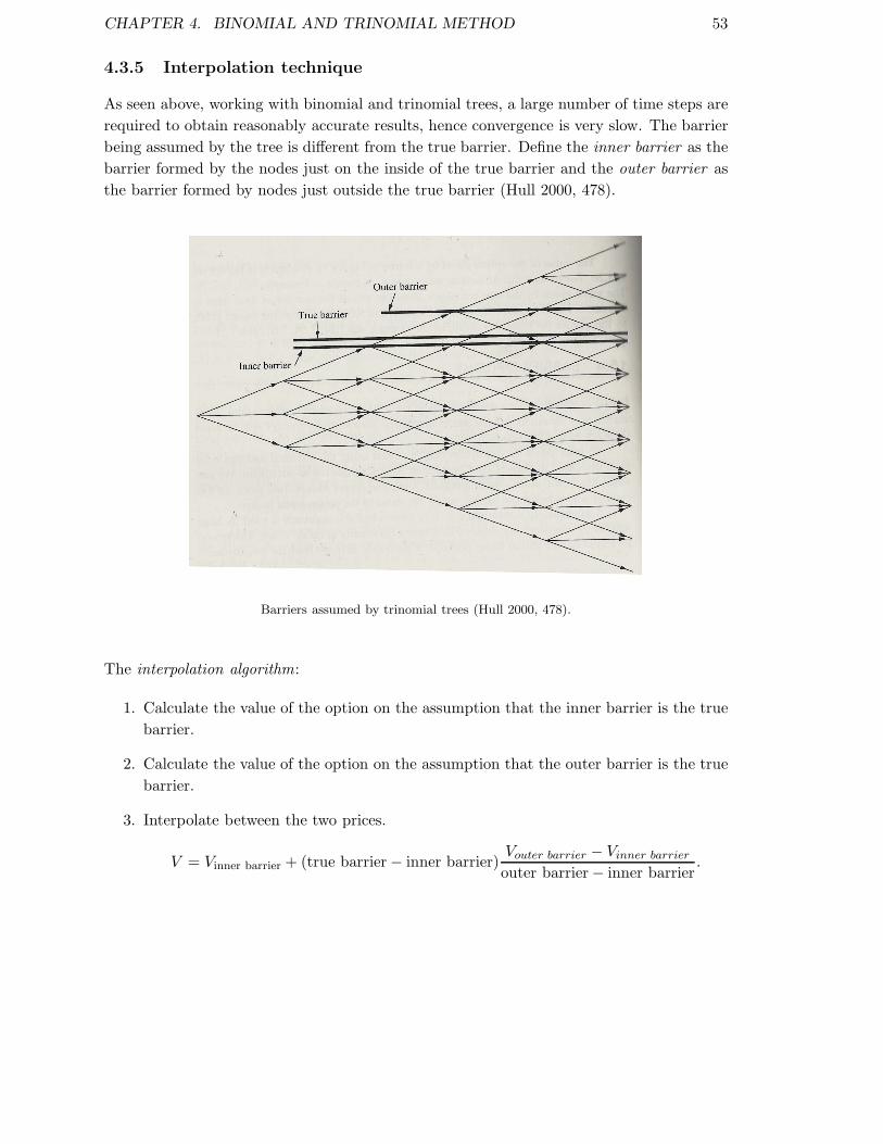
CHAPTER 4. BINOMIAL AND TRINOMIAL METHOD 53
4.3.5 Interpolation technique
As seen above, working with binomial and trinomial trees, a large number of time steps are
required to obtain reasonably accurate results, hence convergence is very slow. The barrier
being assumed by the tree is different from the true barrier. Define the inner barrier as the
barrier formed by the nodes just on the inside of the true barrier and the outer barrier as
the barrier formed by nodes just outside the true barrier (Hull 2000, 478).
Barriers assumed by trinomial trees (Hull 2000, 478).
The interpolation algorithm:
1. Calculate the value of the option on the assumption that the inner barrier is the true
barrier.
2. Calculate the value of the option on the assumption that the outer barrier is the true
barrier.
3. Interpolate between the two prices.
V = Vinner barrier + (true barrier− inner barrier)Vouter barrier − Vinner barrier
outer barrier− inner barrier.

CHAPTER 4. BINOMIAL AND TRINOMIAL METHOD 54
Example 4.3.4 Consider a down-and-out call option and the binomial method, with K >
B; S = 100; K = 95; σ = 0, 3; r = 0, 1; T = 0, 2 and B = 85.
Using CRR (section 4.1) parameters; u = eσ√δt, d = e−σ
√δt and p = (erδt − d)/(u− d), and
substituting the given values; u = 1, 0995, d = 0, 9095 and p = 0, 5292.
Calculating the stock value at every node, one obtains:
First calculate the value of the option on the assumption that the inner barrier
is the true barrier:
Value the options at every point below or equal to the barrier. The values below or equal
to the barrier are equal to zero, thus cn3 = 0 and cn6 = 0
Then calculate the option price at each terminal node by using the payoff equation c(S, t) =
max(S −K, 0), where K =strike price. Thus cn4 = 25, 89 and cn5 = 5.
(For example: cn4 = max(120, 89 − 95; 0) = 25, 89
Then apply backward induction using equations
cn2 = e−rδt(pcn4 + (1− p)cn5);
cn1 = e−rδt(pcn2 + (1− p)cn3)
and substitute the valid numerical data.
(For example: cn2 = e−0,1×0,1(0, 5292 × 25, 89 + (1− 0, 5292) × 5) = 15, 90)
The option value obtained at each node:
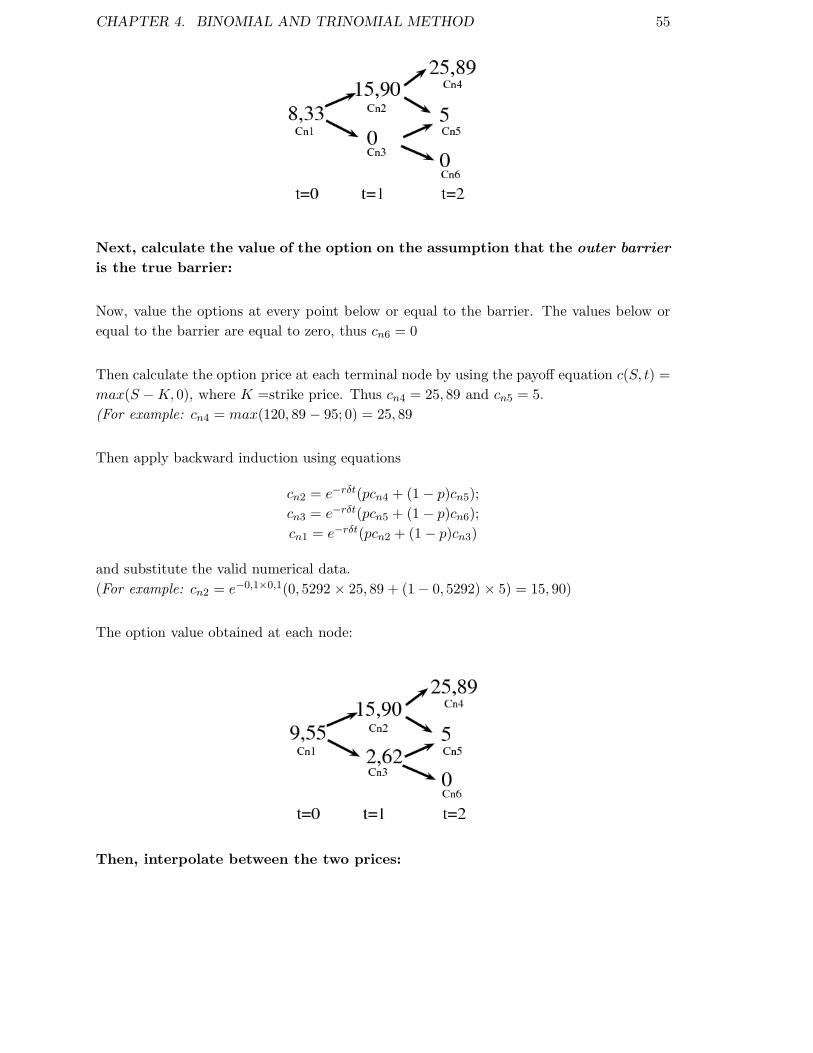
CHAPTER 4. BINOMIAL AND TRINOMIAL METHOD 55
Next, calculate the value of the option on the assumption that the outer barrier
is the true barrier:
Now, value the options at every point below or equal to the barrier. The values below or
equal to the barrier are equal to zero, thus cn6 = 0
Then calculate the option price at each terminal node by using the payoff equation c(S, t) =
max(S −K, 0), where K =strike price. Thus cn4 = 25, 89 and cn5 = 5.
(For example: cn4 = max(120, 89 − 95; 0) = 25, 89
Then apply backward induction using equations
cn2 = e−rδt(pcn4 + (1− p)cn5);
cn3 = e−rδt(pcn5 + (1− p)cn6);
cn1 = e−rδt(pcn2 + (1− p)cn3)
and substitute the valid numerical data.
(For example: cn2 = e−0,1×0,1(0, 5292 × 25, 89 + (1− 0, 5292) × 5) = 15, 90)
The option value obtained at each node:
Then, interpolate between the two prices:
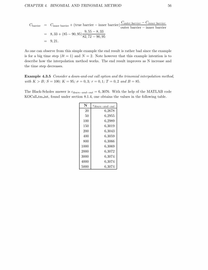
CHAPTER 4. BINOMIAL AND TRINOMIAL METHOD 56
Cbarrier = Cinner barrier + (true barrier− inner barrier)Couter barrier − Cinner barrier
outer barrier− inner barrier
= 8, 33 + (85− 90, 95)9, 55 − 8, 33
82, 72 − 90, 95= 9, 21.
As one can observe from this simple example the end result is rather bad since the example
is for a big time step (δt = 1) and N = 2. Note however that this example intention is to
describe how the interpolation method works. The end result improves as N increase and
the time step decreases.
Example 4.3.5 Consider a down-and-out call option and the trinomial interpolation method,
with K > B; S = 100; K = 95; σ = 0, 3; r = 0, 1; T = 0, 2 and B = 85.
The Black-Scholes answer is cdown−and−out = 6, 3076. With the help of the MATLAB code
KOCall tm int, found under section 8.1.4, one obtains the values in the following table.
N cdown−and−out
20 6,2678
50 6,2955
100 6,2989
150 6,3019
200 6,3043
400 6,3059
800 6,3066
1000 6,3069
2000 6,3072
3000 6,3074
4000 6,3074
5000 6,3074
CHAPTER 4. BINOMIAL AND TRINOMIAL METHOD 57
4.3.6 Stretch technique
This technique is due to the trinomial lattice implementation by (Kamrad & Ritchken 1991).
Since (Kamrad & Ritchken 1991) applied their technique to the logarithm of the underlying
asset, the first step in this section is to explain why it can be done.
Simulation
There are two natural ways to simulate a continuous time price process:
1. Consider the processdS(t)
S(t)= µdt+ σdz.
Then take an interval length δt and set S(t0) = S0 (a given initial price at
t = t0).
The corresponding simulation equation is
S(tk+1)− S(tk) = µS(tk)δt+ σS(tk)ε(tk)√δt,
where the ε(tk) values are uncorrelated normal random variables of mean
0 and standard deviation 1.
This leads to the multiplicative model
S(tk+1) = [1 + µδt+ σε(tk)√δt]S(tk).
The random coefficient is not log normal but normal, thus the simulation
method does not produce log normal price distributions.
2. An alternative approach is to use the log form d lnS(t) = µdt+ σdt.
In discrete form this is
lnS(tk+1)− lnS(tk) = µδt+ σε(tk)√δt.
This leads to the multiplicative model
S(tk+1) = eµδt+σε(tk)√δtS(tk),
with a log normal random coefficient.
The two methods are not exactly equivalent but their differences tend to cancel
in the long run.
Therefore, either method is about as good as the other in practice, (Luenberger
1998). The simulation methods are described in section 5.1.
Assume the log of the underlying asset follows a geometric Wiener process, with drift
µ = r− σ2/2, where r is the riskless rate, and σ is the instantaneous volatility. Then, with
S(t) representing the price at date t, one obtains
ln{S(t+∆t)} = ln{S(t)}+ ξ(t),
CHAPTER 4. BINOMIAL AND TRINOMIAL METHOD 58
with S(0) given, where ξ(t) is a normal random variable with mean µ∆t and variance σ2∆t.
For a parameter λ ≥ 1, define pu, pd and pm as:
pu =1
2λ2+
µ√∆t
2λσ, (4.12)
pd =1
2λ2− µ
√∆t
2λσ, (4.13)
pm = 1− 1
λ2, (4.14)
λ is referred to as the stretch parameter. It can be viewed as a parameter that indicates
the spacing between the underlying movements from one time period to another. If λ = 1
then pm = 0 and the lattice is then a binomial lattice.
For a down-and-out call option one can choose the stretch parameter λ such that the barrier
is hit exactly. η0 is the largest integer smaller then η, where η is given by:
η =ln(S0/B)
σ√∆t
.
If η is an integer, then one shall maintain λ, thus 1 ≤ λ < 2. In most case η is not an
integer, then
η = η0λ.
The resulting algorithm to find λ can be summarized as follows:
Set η =ln(S/B)
σ√∆t
if η > 2
λ = η/ rounded off (η)
else
λ = η
end
Thus
1. Determine λ.
2. Precompute invariant quantities u, d, pu, pm and pd.
3. Calculate stock prices.
4. Calculate option price.
Example 4.3.6 Consider a down-and-out call option with K > B; S = 10; K = 9;
σ = 0, 25; r = 0, 05; T = 1 and B = 5.
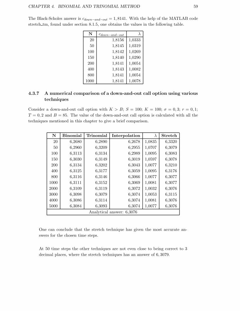
CHAPTER 4. BINOMIAL AND TRINOMIAL METHOD 59
The Black-Scholes answer is cdown−and−out = 1, 8141. With the help of the MATLAB code
stretch tm, found under section 8.1.5, one obtains the values in the following table.
N cdown−and−out λ
20 1,8156 1,0333
50 1,8145 1,0319
100 1,8142 1,0269
150 1,8140 1,0290
200 1,8141 1,0054
400 1,8143 1,0082
800 1,8141 1,0054
1000 1,8141 1,0078
4.3.7 A numerical comparison of a down-and-out call option using various
techniques
Consider a down-and-out call option with K > B; S = 100; K = 100; σ = 0, 3; r = 0, 1;
T = 0, 2 and B = 85. The value of the down-and-out call option is calculated with all the
techniques mentioned in this chapter to give a brief comparison.
N Binomial Trinomial Interpolation λ Stretch
20 6,2680 6,2890 6,2678 1,0835 6,3320
50 6,2960 6,3209 6,2955 1,0707 6,3079
100 6,3113 6,3134 6,2989 1,0095 6,3083
150 6,3030 6,3149 6,3019 1,0597 6,3078
200 6,3134 6,3202 6,3043 1,0077 6,3210
400 6,3125 6,3177 6,3059 1,0095 6,3176
800 6,3116 6,3146 6,3066 1,0077 6,3077
1000 6,3111 6,3152 6,3069 1,0081 6,3077
2000 6,3109 6,3119 6,3072 1,0032 6,3076
3000 6,3098 6,3079 6,3074 1,0053 6,3115
4000 6,3086 6,3114 6,3074 1,0081 6,3076
5000 6,3084 6,3093 6,3074 1,0077 6,3076
Analytical answer: 6,3076
One can conclude that the stretch technique has given the most accurate an-
swers for the chosen time steps.
At 50 time steps the other techniques are not even close to being correct to 3
decimal places, where the stretch techniques has an answer of 6, 3079.
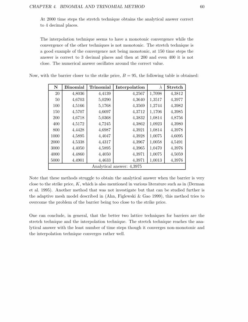
CHAPTER 4. BINOMIAL AND TRINOMIAL METHOD 60
At 2000 time steps the stretch technique obtains the analytical answer correct
to 4 decimal places.
The interpolation technique seems to have a monotonic convergence while the
convergence of the other techniques is not monotonic. The stretch technique is
a good example of the convergence not being monotonic, at 150 time steps the
answer is correct to 3 decimal places and then at 200 and even 400 it is not
close. The numerical answer oscillates around the correct value.
Now, with the barrier closer to the strike price, B = 95, the following table is obtained:
N Binomial Trinomial Interpolation λ Stretch
20 4,8036 4,4139 4,2567 1,7098 4,3812
50 4,6703 5,0290 4,3640 1,3517 4,3977
100 4,5166 5,1768 4,3569 1,2744 4,3982
150 4,5707 4,6697 4,3712 1,1706 4,3985
200 4,6718 5,0368 4,3832 1,0814 4,8756
400 4,5172 4,7245 4,3862 1,0923 4,3980
800 4,4428 4,6987 4,3921 1,0814 4,3978
1000 4,5895 4,4047 4,3928 1,0075 4,6095
2000 4,5338 4,4317 4,3967 1,0058 4,5491
3000 4,4050 4,5895 4,3965 1,0470 4,3976
4000 4,4860 4,4050 4,3971 1,0075 4,5059
5000 4,4901 4,4633 4,3971 1,0013 4,3976
Analytical answer: 4,3975
Note that these methods struggle to obtain the analytical answer when the barrier is very
close to the strike price, K, which is also mentioned in various literature such as in (Derman
et al. 1995). Another method that was not investigate but that can be studied further is
the adaptive mesh model described in (Ahn, Figlewski & Gao 1999), this method tries to
overcome the problem of the barrier being too close to the strike price.
One can conclude, in general, that the better two lattice techniques for barriers are the
stretch technique and the interpolation technique. The stretch technique reaches the ana-
lytical answer with the least number of time steps though it converges non-monotonic and
the interpolation technique converges rather well.
CHAPTER 4. BINOMIAL AND TRINOMIAL METHOD 61
4.4 Discrete barrier options
A barrier can be either continuous or discrete. Once a continuously monitored barrier is
reached the option is immediately knocked in or out, while in discretely monitored condi-
tions, barriers only come into effect in discrete monitored time, for example at close of every
market day, every quarter, every month, or every half year (Wilmott 2007, 372).
Barrier monitoring is often assumed to be continuous, but in practice it is often discrete,
which may lead to significant pricing errors, (Forsyth, Vetzal & Zvan 2000). In the continu-
ous time, the payoffs depend on the price of the underlying asset throughout the life of the
option. While in discrete time, the payoffs are determined by underlying prices at a finite
set of time, (Broadie, Glasserman & Kou 1999).
Discretely monitored barrier options are popular and important, although pricing them
is not as easy as their continuous counterparts. There is in essence no direct analytical
solution. Many traded options are based on discrete price, though nearly all closed-form
expressions available for pricing path-dependent options are based on continuous-time paths,
(Broadie et al. 1999). Thus, in this chapter the question becomes how best to use a contin-
uous formula to approximate the price of a discrete barrier option.
4.4.1 The barrier adjustment technique for Black-Scholes
This method developed by (Broadie et al. 1997) shows that discrete barrier options can be
priced with remarkable accuracy using continuous barrier formulas by applying a simple
continuity correction to the barrier (B). The method utilizes the formulae for the prices
of continuous barrier options, but shifts the barrier to correct for discrete monitoring by
adapting the barrier to:
Bnew = Be±ασ
√
T
m , (4.15)
where
CHAPTER 4. BINOMIAL AND TRINOMIAL METHOD 62
α = αup or αdown,
αup = 0, 5863 (for a up barrier),
αdown = −0, 5826 (for a down barrier),
B = Barrier,
σ = volatility,
T = time period,
m = number of times the underlying asset price is monitored over [0, T ].
The shift is determined exclusively by the asset volatility, a constant α and the monitoring
frequency, (Broadie et al. 1997). Equation (4.15), the adjustment to the barrier, pushes the
barrier away from the initial stock price to compensate for the excessive frequency of the
barrier being breached when observations are continuous. For each time interval δt on the
interval [0, T ], check whether the Barrier has been hit.
Example 4.4.1 Consider a discrete down-and-out call option with K > B; S = 100;
K = 100; σ = 0, 3; r = 0, 1; T = 0, 2 B = 85 and m = 50.
The program in section 8.1.1 is used with the adjusted barrier Bnew = Be±ασ
√
T
m .
Once again the Black-Scholes formula for this option is given by:
cdown−out = S(N(d1)− b(1−N(d8)))−Ke−r(T )(N(d2)− a(1−N(d7)))
where
d1 =log(S/K) + (r + 1
2σ2)(T )
σ√T
,
d2 =log(S/K) + (r − 1
2σ2)(T )
σ√T
,
d7 =log(SK/B2
new)− (r − 12σ
2)(T )
σ√T
,
d8 =log(SK/B2
new)− (r + 12σ
2)(T )
σ√T
.
CHAPTER 4. BINOMIAL AND TRINOMIAL METHOD 63
The option value is cdown−out = 6, 32213.
The result is similar to the result obtained in (Broadie et al. 1997). Note that the discrete
answer is higher than the continuous answer obtained in section 3.2. When a continuously
monitored barrier is reached the option is immediately knocked in or out, while in discretely
monitored conditions, barriers only come into effect in discrete monitored time.
4.4.2 The barrier adjustment technique for the trinomial method
Numerical methods are necessary for accurate evaluation of discrete option prices. They are
based on discretization of time, but typically a much finer one than specified in the terms
of an option. One has to adapt the time discretization for a discrete option, the process
involves two time increments, (Broadie et al. 1999):
� the time intervals between the monitory times,
� the time steps of the numerical method.
Hence when adapting the trinomial method for a discrete barrier option, N (the number of
time steps in the tree diagram), should be divisible by m (the number of monitoring times),
(Broadie et al. 1999).
This section discusses a correction term that improves the approximation of discrete-time
barrier options. The correction shifts the barrier to price a discrete option using the trino-
mial method for continuous monitored barriers.
(Broadie et al. 1999) adapted the techniques of (Boyle & Lau 1994), (Kamrad & Ritchken
1991) and (Ritchken 1995) that were discussed in chapter 4.
In the case of a discrete barrier option, one can use a trinomial method that puts a row
of nodes at the level of the shifted barrier. Thus, making use of the stretch technique in
section 4.3.6 and article, (Broadie et al. 1999).
Then we adapt the pricing algorithm in (Broadie et al. 1999) as follows:
1. Determine λ
Set η =ln(S/B)
σ√∆t
if η > 2

CHAPTER 4. BINOMIAL AND TRINOMIAL METHOD 64
λ = η/ rounded off (η)
else
λ = η
end
2. Precompute invariant quantities u, d, pu, pm and pd
u = eλσ
√
T
N
d = e−λσ
√
T
N
pu =1
2λ2+
(r − σ2
2 )√
TN
2λσ
pm = 1− 1
λ2
pd = 1− pu − pm
3. Calculate stock prices on the nodes of the tree.
4. Set Bnew = Be±0,5λ
√
T
m , where B is the initial barrier. For an up option use
Bnew = Be0,5λ
√
T
m
and for a down option use
Bnew = Be−0,5λ
√
T
m .
5. Calculate option price with the discrete shift barrier (Bnew), similar to the technique
described in section 4.3.6.
Example 4.4.2 Consider a down-and-out call option with K > B; S = 100; K = 100;
σ = 0, 3; r = 0, 1; T = 0, 2 B = 85 and m = 50.
The program in section 8.1.5 is used with the adjusted barrier Bnew = Be±0,5λ
√
T
m .
N λ cdown−out
100 1,0095 6,3250
200 1,0077 6,3295
300 1,0491 6,3271
400 1,0095 6,3249
500 1,0032 6,3234
1000 1,0081 6,3241
1500 1,0199 6,3218
2000 1,0032 6,3233
2500 1,0095 6,3221
3000 1,0053 6,3210
True value: 6,3221
CHAPTER 4. BINOMIAL AND TRINOMIAL METHOD 65
The ”true” value is determined from the modified trinomial procedure described in (Broadie
et al. 1999). In order to compute the true value to within 0, 001 on average, this modified
trinomial procedure needs to run the routine using 80000 time steps, according to (Broadie
et al. 1997).
In (Broadie et al. 1999) the algorithm is adapted to find another set of values for λ and N ,
to improve the results. However, the algorithm is not described in detail and could not be
tested.
When one experiments with the example in table 1 of (Broadie et al. 1999), using S = K =
100, B = 95, σ = 0, 6, r = 0, 1, m = 3 and T = 0, 2 and our algorithm, one obtains for
N = 504; λ = 1, 0728 and cdown−out = 9, 461.
The result compares sufficiently with their algorithm since for N = 504 their answer is
cdown−out = 9, 493.
Chapter 5
Monte Carlo Method
5.1 Monte Carlo simulation
Option value calculations can be regarded as calculating expected values. The Monte Carlo
method calculates the expected values of random variables.
The basic principle of pricing options via Monte Carlo simulation can be described as; ”the
value of an option is the present value of the expected payoff under a risk neutral random
walk” (Wilmott 2007, 338).
The method can be extended to calculate option values where payoffs depend on several
market variables. Monte Carlo simulation is one of the most powerful and most easily im-
plemented methods for the calculation of option values. It provides a method to compute
option values in cases where no analytical formulas are available. However, it is computa-
tionally expensive and cannot handle American style options with ease, (Hull 2000, 406).
Generally the method first simulates sample paths of the underlying asset over the relevant
time interval. Then it simulates these according to the risk-neutral measure. Subsequently
the method evaluates the discounted cash flows of a security on each sample path, it averages
the discounted cash flows over the sample paths.
Generating option paths:
Assuming that the underlying stock S follows a geometric brownian motion, one finds the
stochastic differential equation (SDE) for the stock return to be (Hull 2000, 407)
dS = µSdt+ σSdW, (5.1)
where µ is the expected return, σ is the volatility and dW the Weiner process. To simulate
66
CHAPTER 5. MONTE CARLO METHOD 67
one path for S one has to divide the lifespan of the option into M intervals of length δt
(process of discretization), and approximate (5.1) by
δt → 0, S(t+ δt)− S(t) = µS(t)δt+ σS(t)ε√δt.
Where
S(t) : Stock price at time t,
S(t+ δt) : Stock price at one time interval,
ε : A random value from a sample from the normal distribution with mean zero, and stan-
dard deviation one,
δt : Interval length.
Refer back to section 2.2.3 on page 9 and apply formula
df =
[
µSt∂f
∂S+
1
2σ2S2
t
∂2f
∂S2+
∂f
∂t
]
dt+ σSt∂f
∂SdWt,
to the function
f(S, t) = lnS.
Thus in this case
∂f
∂S(St, t) =
1
St,
∂f
∂t(St, t) = 0,
∂2f
∂S2(St, t) = − 1
S2t
,
and the result is
d(lnSt) =
[
µSt1
St− 1
2σ2S2
t
1
S2t
]
dt+ σSt1
StdWt (5.2)
=
[
µ− 1
2σ2
]
dt+ σdWt. (5.3)
Thus d(log St) is normally distributed with mean[
µ− 12σ
2]
dt and variance σ2dt, (Roman
2004).
Since the underlying option’s returns follow a log normal distribution, applying Ito’s lemma
as above, leads to (5.3), so that
lnS(t+ δt) − lnS(t) =
(
µ− 1
2σ2
)
δt+ σε√δt, (5.4)

CHAPTER 5. MONTE CARLO METHOD 68
or
S(t+ δt) = S(t)e(µ−1
2σ2)δt+σε
√δt. (5.5)
The more time steps that are used in the model and the smaller the time steps size are in
the model, the closer the model comes to a real asset price movement.
The pricing algorithm (Wilmott 2007, 924) :
1. Assume that σ and r (risk-free interest rate), are known. Simulate the risk-neutral
random walk starting at today’s value of the stock over the required time horizon.
This gives one realization of the underlying price path.
2. For this realization calculate the option payoff.
3. Perform many more such realizations over the time horizon.
4. Calculate the average payoff over all realizations.
5. Take the present value of this average, this is the option value.
for i = 1 to M
compute an N(0,1) sample εi
set Si = S0e(r− 1
2σ2)T+σ
√Tεi
set Vi = e−rTΛ(Si)
end
set aM = 1M
∑Mi=1 Vi
set b2M =(
1(M−1)
)
∑Mi=1(Vi − aM )2
Where Λ(x) denotes the payoff function, such that Λ(x) = max(x − E, 0) for a call and
Λ(x) = max(x− E, 0) for a put (Higham 2004, 115).
The output provides an approximate option price aM and an approximate 95% confidence
interval using the formula
[
aM − 1, 96bM√M
,aM +1, 96bM√
M
]
,
aM is the price of the option (Higham 2004).

CHAPTER 5. MONTE CARLO METHOD 69
5.1.1 Advantages of Monte Carlo
1. The mathematics needed to perform Monte Carlo simulations are simple.
2. The model can be adjusted without too much trouble.
3. To get a better accuracy, one just has to run more simulations.
4. The technique readily carries over to some European exotic and path-dependent con-
tracts.
5.1.2 Disadvantages of Monte Carlo
1. A limitation that typically makes it impossible to get very high accuracy from a Monte
Carlo approximation, is that the size of the confidence interval shrinks like the inverse
square root of the number of samples. To reduce the ’error’ by a factor of 10 requires
a hundredfold increase in the sample size. Hence quite a large M is necessary to
simulate the different paths to obtain accurate prices (Higham 2004, 143).
2. The Monte Carlo method in its basic form is only used to estimate the option price
at one point in S. With American options, to know when it is optimal to exercise the
option, one must calculate the option price for all values of S and t up to expiry in
order to check that at no time there is arbitrage opportunities. Thus the Monte Carlo
application to American options is far from straightforward (Higham 2004, 196).
3. The square root of the variance, of the random variable under consideration is the size
of the confidence interval, which is directly proportional to the standard deviation. It
is highly desirable in practice to use the technique variance reduction, which occurs
in section 5.3. This technique transforms the problem E(X) to the problem of E(Y )
where Y is another random sample that has the same mean as X, but a smaller
variance (Higham 2004, 143).
CHAPTER 5. MONTE CARLO METHOD 70
5.2 Barrier options
The Monte Carlo method extends easily to handle path dependency options such as Barrier
Options.
The following algorithm values a down-and-out call option. Here, M is the number of asset
paths that are sampled.
for i = 1 to M
for j = 0 to N − 1
compute an N(0,1) sample εj
set Sj+1 = Sje(r− 1
2σ2)∆t+σ
√∆tεj
end
set Smaxi = max0≤j≤NSj
if Smaxi > B
set Vi = e−rTmax(SN −K, 0),
else set Vi = 0
end
set aM = 1M
∑Mi=1 Vi
set b2M =(
1(M−1)
)
∑Mi=1(Vi − aM )2
The result gives an approximate option price aM and an approximate 95% confidence in-
terval using the formula,[
aM − 1, 96bM√M
,aM +1, 96bM√
M
]
(Higham 2004, 194).
Example 5.2.1 Consider a down-and-out call option with K > B; S = 100; K = 100;
σ = 0, 3; r = 0, 1; T = 0, 2 and B = 85, where CI is the confidence interval.
The Black-Scholes answer is cdown−and−out = 6, 3076. With the help of the MATLAB code
monte(S,K,sigma,r,T,Dt,N,M) found in section 8.1.6, one obtains the values in the following
table.
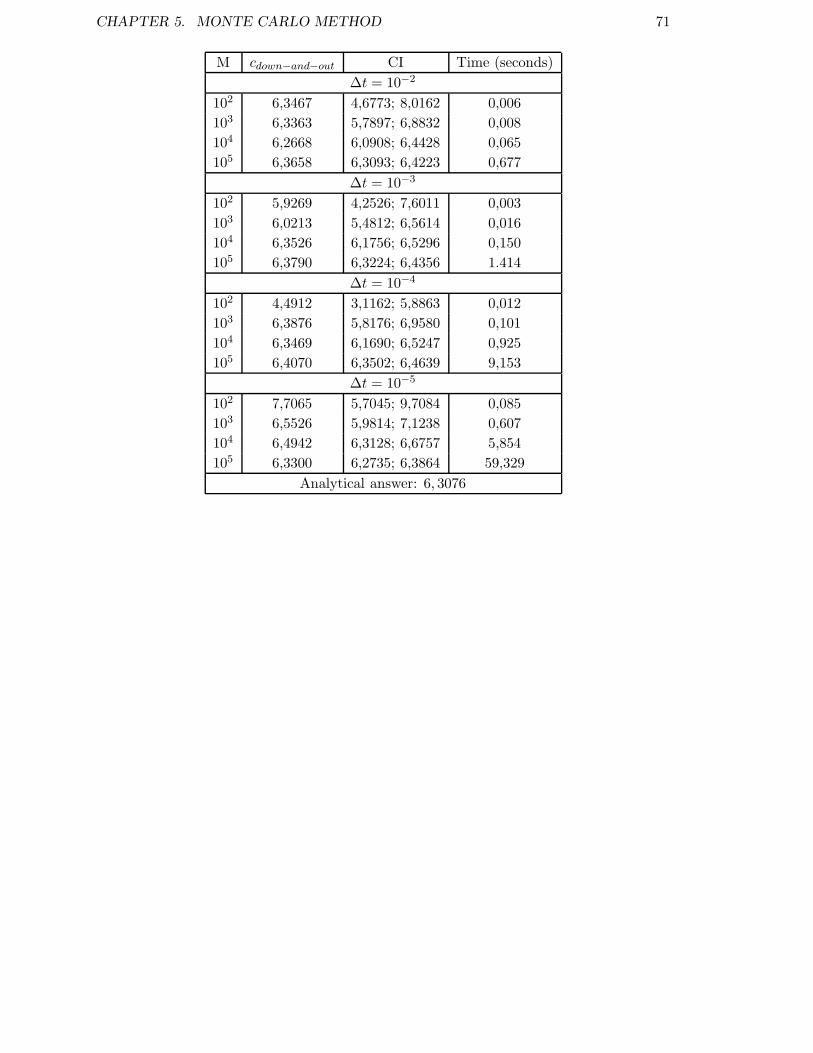
CHAPTER 5. MONTE CARLO METHOD 71
M cdown−and−out CI Time (seconds)
∆t = 10−2
102 6,3467 4,6773; 8,0162 0,006
103 6,3363 5,7897; 6,8832 0,008
104 6,2668 6,0908; 6,4428 0,065
105 6,3658 6,3093; 6,4223 0,677
∆t = 10−3
102 5,9269 4,2526; 7,6011 0,003
103 6,0213 5,4812; 6,5614 0,016
104 6,3526 6,1756; 6,5296 0,150
105 6,3790 6,3224; 6,4356 1.414
∆t = 10−4
102 4,4912 3,1162; 5,8863 0,012
103 6,3876 5,8176; 6,9580 0,101
104 6,3469 6,1690; 6,5247 0,925
105 6,4070 6,3502; 6,4639 9,153
∆t = 10−5
102 7,7065 5,7045; 9,7084 0,085
103 6,5526 5,9814; 7,1238 0,607
104 6,4942 6,3128; 6,6757 5,854
105 6,3300 6,2735; 6,3864 59,329
Analytical answer: 6, 3076
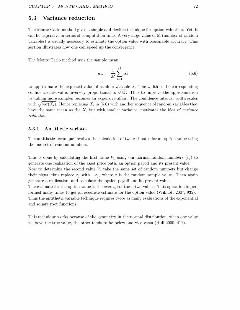
CHAPTER 5. MONTE CARLO METHOD 72
5.3 Variance reduction
The Monte Carlo method gives a simple and flexible technique for option valuation. Yet, it
can be expensive in terms of computation time. A very large value of M (number of random
variables) is usually necessary to estimate the option value with reasonable accuracy. This
section illustrates how one can speed up the convergence.
The Monte Carlo method uses the sample mean
am :=1
M
M∑
i=1
Xi (5.6)
to approximate the expected value of random variable X. The width of the corresponding
confidence interval is inversely proportional to√M . Thus to improve the approximation
by taking more samples becomes an expensive affair. The confidence interval width scales
with√
var(Xi). Hence replacing Xi in (5.6) with another sequence of random variables that
have the same mean as the Xi but with smaller variance, motivates the idea of variance
reduction.
5.3.1 Antithetic variates
The antithetic technique involves the calculation of two estimates for an option value using
the one set of random numbers.
This is done by calculating the first value V1 using our normal random numbers (εj) to
generate one realization of the asset price path, an option payoff and its present value.
Now to determine the second value V2 take the same set of random numbers but change
their signs, thus replace εj with −εj , where ε is the random sample value. Then again
generate a realization, and calculate the option payoff and its present value.
The estimate for the option value is the average of these two values. This operation is per-
formed many times to get an accurate estimate for the option value (Wilmott 2007, 935).
Thus the antithetic variable technique requires twice as many evaluations of the exponential
and square root functions.
This technique works because of the symmetry in the normal distribution, when one value
is above the true value, the other tends to be below and vice versa (Hull 2000, 411).
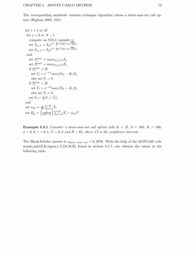
CHAPTER 5. MONTE CARLO METHOD 73
The corresponding antithetic variates technique algorithm values a down-and-out call op-
tion (Higham 2004, 224):
for i = 1 to M
for j = 0 to N − 1
compute an N(0,1) sample εj
set Sj+1 = Sje(r− 1
2σ2)∆t+σ
√∆tξj
set Sj+1 = Sje(r− 1
2σ2)∆t−σ
√∆tξj
end
set Smaxi = max0≤j≤NSj
set Smaxi = max0≤j≤N Sj
if Smaxi > B
set Vi = e−rTmax(SN −K, 0),
else set Vi = 0
if Smaxi > B
set Vi = e−rTmax(SN −K, 0),
else set Vi = 0
set Vi =12(Vi + Vi)
end
set aM = 1M
∑Mi=1 Vi
set b2M =(
1(M−1)
)
∑Mi=1(Vi − aM )2
Example 5.3.1 Consider a down-and-out call option with K > B; S = 100; K = 100;
σ = 0, 3; r = 0, 1; T = 0, 2 and B = 85, where CI is the confidence interval.
The Black-Scholes answer is cdown−and−out = 6, 3076. With the help of the MATLAB code
monte anti(S,K,sigma,r,T,Dt,M,B) found in section 8.1.7, one obtains the values in the
following table.

CHAPTER 5. MONTE CARLO METHOD 74
M cdown−and−out CI Time (seconds)
∆t = 10−2
102 6,8449 5,8947; 7,7951 0,016
103 6,4445 6,1619; 6,7272 0,033
104 6,3448 6,2545; 6,4351 0,162
105 6,3385 6,3098; 6,3671 1,306
∆t = 10−3
102 6,2356 5,3459; 7,1252 0,009
103 6,2455 5,9701; 6,5208 0,049
104 6,2696 6,1801; 6,3591 0,294
105 6,3453 6,3166; 6,3741 2,698
∆t = 10−4
102 5,2406 4,5647; 5,9166 0,041
103 6,1168 5,8361; 6,3975 0,222
104 6,2447 6,1545; 6,3349 1,682
105 6,3483 6,3195; 6,3771 16,438
∆t = 10−5
102 6,8957 5,9602; 7,8311 0,168
103 6,2186 5,9422; 6,4948 1,146
104 6,3099 6,2185; 6,4013 10,311
105 6,3228 6,2942; 6,3515 97,908
Analytical answer: 6, 3076
5.3.2 Comparison
∆t = 10−5
M cdown−and−out CI Time (seconds)
Monte Carlo Simulation
102 7,7065 5,7045; 9,7084 0,085
103 6,5526 5,9814; 7,1238 0,607
104 6,4942 6,3128; 6,6757 5,854
105 6,3300 6,2735; 6,3864 59,329
Antithetic Variable Technique
102 6,8957 5,9602; 7,8311 0,168
103 6,2186 5,9422; 6,4948 1,146
104 6,3099 6,2185; 6,4013 10,311
105 6,3228 6,2942; 6,3515 97,908
Analytical answer: 6, 3076
At M = 104 the standard Monte Carlo simulation confidence interval does not even include

CHAPTER 5. MONTE CARLO METHOD 75
the correct answer, whereas the antithetic variable technique has an answer of 6,3099.
One can conclude that the antithetic variable technique has given more accurate answers
in comparison to the standard Monte Carlo simulation. Observe that the technique shrinks
the confidence intervals. However, twice as many evaluations of the exponential and square
root functions are required (Higham 2004, 218).
The control variate technique is another variance reduction method that one can study
further.
It is important to note that the overall accuracy of the Monte Carlo process depends not
only on the error in the Monte Carlo approximation to the mean, but also on the error
arising from the time discretization. (Higham 2004, 224).
Example 5.3.2 Consider a down-and-out call option with K > B; S = 10; K = 9;
σ = 0, 25; r = 0, 05; T = 1 and B = 5.
M δt = 10−3 δt = 10−4
Monte Carlo Simulation
104 1,8241 1,8527
105 1.8279 1.8137
Antithetic Variable Technique
104 1,8068 1,8085
105 1.8133 1.8088
Analytical answer: 1, 8141
Chapter 6
Finite Difference Methods
Finite difference methods are designed for finding numerical solutions of differential equa-
tions. They value a derivative by solving the differential equation that the derivative satis-
fies.
The finite difference method involves converting the Black-Scholes differential equation into
a set of algebraic equations which can then be solved numerically using an appropriate
technique. Consider the Black-Scholes differential equation
∂f
∂t+ rS
∂f
∂S+
1
2σ2S2 ∂
2f
∂S2= rf. (6.1)
Where
f = the option value,
S = the value of the underlying asset at time t,
r = the risk-free interest rate,
σ = constant volatility.
The finite difference method can calculate, with increased computational effort, option
prices in cases where there are several state variables.
To solve the partial difference equation (PDE) by finite difference methods one must set up
a discrete grid, with respect to time and asset prices.
Note that for the discretization process and the algorithm, the notation f(t, S) is used to
indicate the option value at time t, if the asset price is S(t), to fit the explanation in Hull
(Hull 2000).
Let T be option maturity, divide this into N equally spaced intervals of length δt = T/N .
Let Smax be a suitably large asset price, that one assumes cannot be reached by S(t) within
76
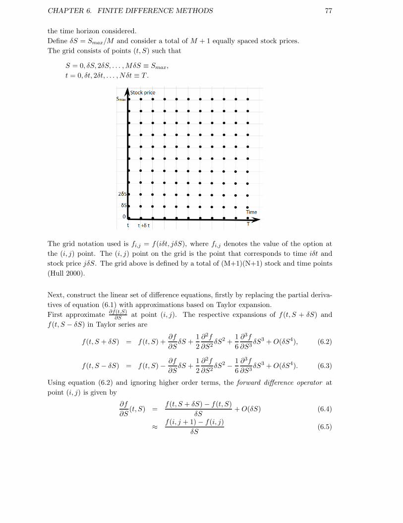
CHAPTER 6. FINITE DIFFERENCE METHODS 77
the time horizon considered.
Define δS = Smax/M and consider a total of M + 1 equally spaced stock prices.
The grid consists of points (t, S) such that
S = 0, δS, 2δS, . . . ,MδS ≡ Smax,
t = 0, δt, 2δt, . . . , Nδt ≡ T .
The grid notation used is fi,j = f(iδt, jδS), where fi,j denotes the value of the option at
the (i, j) point. The (i, j) point on the grid is the point that corresponds to time iδt and
stock price jδS. The grid above is defined by a total of (M+1)(N+1) stock and time points
(Hull 2000).
Next, construct the linear set of difference equations, firstly by replacing the partial deriva-
tives of equation (6.1) with approximations based on Taylor expansion.
First approximate ∂f(t,S)∂S at point (i, j). The respective expansions of f(t, S + δS) and
f(t, S − δS) in Taylor series are
f(t, S + δS) = f(t, S) +∂f
∂SδS +
1
2
∂2f
∂S2δS2 +
1
6
∂3f
∂S3δS3 +O(δS4), (6.2)
f(t, S − δS) = f(t, S)− ∂f
∂SδS +
1
2
∂2f
∂S2δS2 − 1
6
∂3f
∂S3δS3 +O(δS4). (6.3)
Using equation (6.2) and ignoring higher order terms, the forward difference operator at
point (i, j) is given by
∂f
∂S(t, S) =
f(t, S + δS)− f(t, S)
δS+O(δS) (6.4)
≈ f(i, j + 1)− f(i, j)
δS(6.5)
CHAPTER 6. FINITE DIFFERENCE METHODS 78
and similarly using equation (6.3), the corresponding backward difference operator is given
by
∂f
∂S(t, S) =
f(t, S)− f(t, S − δS)
δS+O(δS2) (6.6)
≈ f(i, j) − f(i, j − 1)
δS. (6.7)
Secondly discretize the equations. Subtracting equation (6.3) from (6.2) and taking the first
order partial derivatives results in the central difference operator at point (i, j) given by
∂f
∂S(t, S) =
f(t, S + δS) − f(t, S − δS)
2δS+O(δS3) (6.8)
≈ f(i, j + 1)− f(i, j − 1)
2δS. (6.9)
Then adding equation (6.2) and (6.3), take the second order partial derivative and approx-
imate∂2f
∂S2at the point (i, j) to obtain
∂2f
∂S2(t, S) =
f(t, S + ∂S)− 2f(t, S) + f(t, S − δS)
δS2+O(δS3) (6.10)
≈ f(i, j + 1)− 2f(i, j) + f(i, j − 1)
δS2. (6.11)
This approximation is preferred because its symmetry preserves the reflectional symmetry
of the second order partial derivative.
Approximate f(t+ ∂t, S) at point (i, j) using Taylor series to obtain
f(t+ ∂t, S) = f(t, S) +∂f
∂tδt+
1
2
∂2f
∂t2δt2 +
1
6
∂3f
∂t3δt3 +O(δt4). (6.12)
Thus, the forward difference operator for time is then given by
∂f
∂t(t, S) =
f(t+ δt, S) − f(t, S)
δt+O(δt) (6.13)
≈ f(i+ 1, j) − f(i, j)
δt. (6.14)
To identify the 3 different approaches within the finite difference method,
1. Implicit method
2. Explicit method
3. Crank-Nicolson method
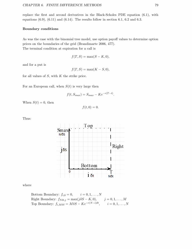
CHAPTER 6. FINITE DIFFERENCE METHODS 79
replace the first and second derivatives in the Black-Scholes PDE equation (6.1), with
equations (6.9), (6.11) and (6.14). The results follow in section 6.1, 6.2 and 6.3.
Boundary conditions
As was the case with the binomial tree model, use option payoff values to determine option
prices on the boundaries of the grid (Brandimarte 2006, 477).
The terminal condition at expiration for a call is
f(T, S) = max(S −K, 0),
and for a put is
f(T, S) = max(K − S, 0),
for all values of S, with K the strike price.
For an European call, when S(t) is very large then
f(t, Smax) = Smax −Ke−r(T−t).
When S(t) = 0, then
f(t, 0) = 0.
Thus:
where
Bottom Boundary: fi,0 = 0, i = 0, 1, . . . , N
Right Boundary: fNδt,j = max(jδS −K, 0), j = 0, 1, . . . ,M
Top Boundary: fi,MδS = MδS −Ke−r(N−i)δt, i = 0, 1, . . . , N
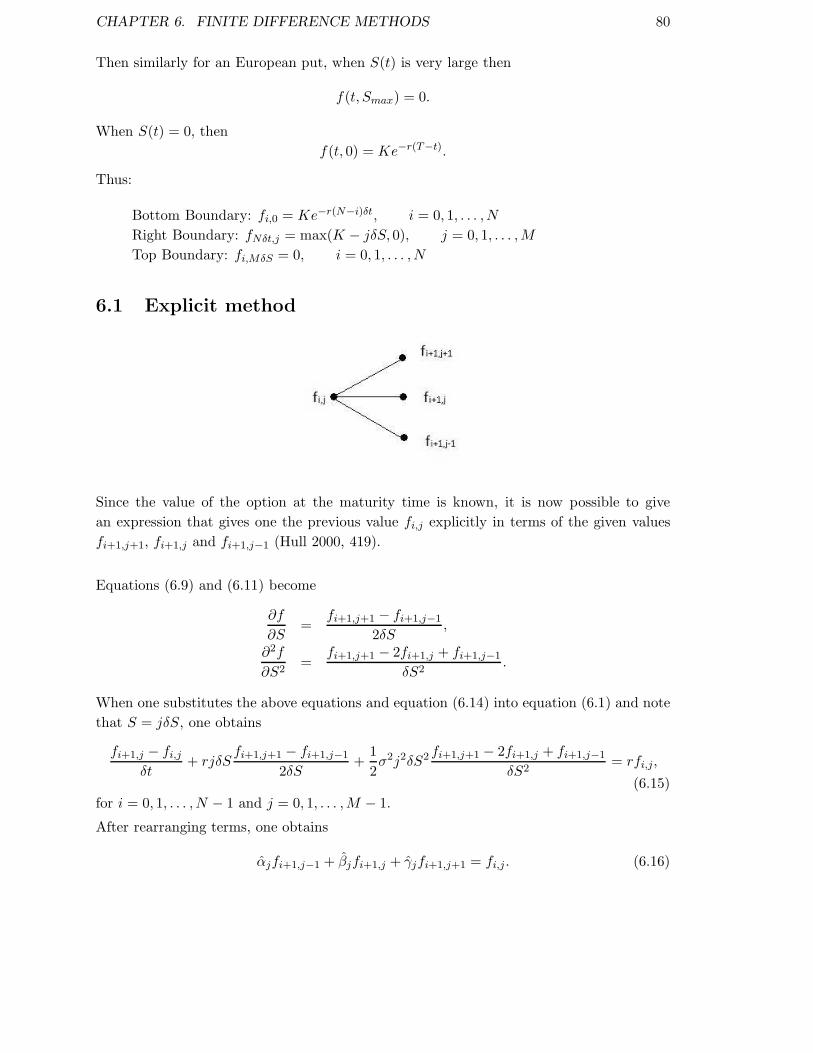
CHAPTER 6. FINITE DIFFERENCE METHODS 80
Then similarly for an European put, when S(t) is very large then
f(t, Smax) = 0.
When S(t) = 0, then
f(t, 0) = Ke−r(T−t).
Thus:
Bottom Boundary: fi,0 = Ke−r(N−i)δt, i = 0, 1, . . . , N
Right Boundary: fNδt,j = max(K − jδS, 0), j = 0, 1, . . . ,M
Top Boundary: fi,MδS = 0, i = 0, 1, . . . , N
6.1 Explicit method
Since the value of the option at the maturity time is known, it is now possible to give
an expression that gives one the previous value fi,j explicitly in terms of the given values
fi+1,j+1, fi+1,j and fi+1,j−1 (Hull 2000, 419).
Equations (6.9) and (6.11) become
∂f
∂S=
fi+1,j+1 − fi+1,j−1
2δS,
∂2f
∂S2=
fi+1,j+1 − 2fi+1,j + fi+1,j−1
δS2.
When one substitutes the above equations and equation (6.14) into equation (6.1) and note
that S = jδS, one obtains
fi+1,j − fi,jδt
+ rjδSfi+1,j+1 − fi+1,j−1
2δS+
1
2σ2j2δS2 fi+1,j+1 − 2fi+1,j + fi+1,j−1
δS2= rfi,j,
(6.15)
for i = 0, 1, . . . , N − 1 and j = 0, 1, . . . ,M − 1.
After rearranging terms, one obtains
αjfi+1,j−1 + βjfi+1,j + γjfi+1,j+1 = fi,j. (6.16)
CHAPTER 6. FINITE DIFFERENCE METHODS 81
Where
αj =1
1 + rδt
(
−1
2rjδt+
1
2σ2j2δt
)
,
βj =1
1 + rδt
(
1− σ2j2δt)
,
γj =1
1 + rδt
(
1
2rjδt+
1
2σ2j2δt
)
.
Equation 6.16 for i = 0, 1, 2, . . . , N − 1 and j = 0, 1, 2, . . . ,M − 1 gives rise to a tridiagonal
system. This results to the tridiagonal system given by
α0 β0α1 β1 γ1
α2 β2 γ2. . . . . .
αM−2 βM−2 γM−2
αM−1 βM−1
fi+1,0
fi+1,1
fi+1,2...
fi+1,M−2
fi+1,M−1
=
fi,0fi,1fi,2...
fi,M−2
fi,M−1
.
The vector of asset prices fi+1,j is known at time T from our initial condition. The value
of the option obtained at time zero is obtained by backward iterations.
It is easy to implement and program this method. However, the method is unstable if the
ratio δt/(δS)2 ≤ 1/2 is not met, and the method is slow to converge (Wilmott 2007, 918)
(Higham 2004, 294).
6.2 Implicit method
When one substitutes equations (6.9), (6.11) and (6.14) into equation (6.1) and note that
S = jδS (Hull 2000, 417), one obtains
fi+1,j − fi,jδt
+ rjδSfi,j+1 − fi,j−1
2δS+
1
2σ2j2δS2 fi,j+1 − 2fi,j + fi,j−1
δS2= rfi+1,j, (6.17)
for i = 0, 1, . . . , N − 1 and j = 0, 1, . . . ,M − 1.
After rearranging terms, one obtains
αjfi,j−1 + βjfi,j + γjfi,j+1 = fi+1,j. (6.18)
CHAPTER 6. FINITE DIFFERENCE METHODS 82
Where
αj =1
2rjδt− 1
2σ2j2δt,
βj = 1 + σ2j2δt+ rδt,
γj = −1
2rjδt− 1
2σ2j2δt.
Equation (6.18) gives rise to a tridiagonal system written as Ax = b, which results in the
tridiagonal system given by
β0 γ0α1 β1 γ1
α2 β2 γ2. . . . . .
αM−2 βM−2 γM−2
αM−1 βM−1
fi,0fi,1fi,2...
fi,M−2
fi,M−1
=
fi+1,0
fi+1,1
fi+1,2...
fi+1,M−2
fi+1,M−1
.
To compute fi,j, j = 0, 1, . . . ,M − 1 the above system for a given fi+1,j, j = 0, 1, . . . ,M is
solved. Start at time t = i+1 = Nδt, using the boundary conditions, and solve the system
of linear equations to obtain the price at time t = i.
Using the newly obtained values at time t = i, one can repeat the process to calculate the
solution at time t = i− 1 until the asset price at time t = 0 is reached.
The system of linear equations can be solved using either the LU decomposition method
(such as Thomas algorithm, section 6.3) or iterative methods (Gauss-Seidel, (Cheney &
Kincaid 2004)).
The implicit method is stable, the method for any solution results in δt/(δS)2 > 0, (Higham
2004).
6.3 Crank-Nicolson method
The Crank-Nicolson finite difference method is the average of the implicit and explicit
methods and is introduced to improve accuracy and is unconditionally stable, hence it gives
results for any ratio δt/(δS)2 > 0, (Higham 2004).
We adapt the method in (Brandimarte 2006) to the grid in (Hull 2000) to derive the fol-
lowing equations.
The implicit scheme is given by equation (6.15) and the explicit scheme by equation (6.17).

CHAPTER 6. FINITE DIFFERENCE METHODS 83
Take the average of the two equations;
1
2
(
fi+1,j − fi,jδt
+ rjδSfi+1,j+1 − fi+1,j−1
2δS+
1
2σ2j2δS2 fi+1,j+1 − 2fi+1,j + fi+1,j−1
δS2= rfi,j
)
,
and
1
2
(
fi+1,j − fi,jδt
+ rjδSfi,j+1 − fi,j−1
2δS+
1
2σ2j2δS2 fi,j+1 − 2fi,j + fi,j−1
δS2= rfi+1,j
)
.
Then one obtains,
fi+1,j − fi,jδt
+rjδS
2
(
fi,j+1 − fi,j−1
2δS
)
+rjδS
2
(
fi+1,j+1 − fi+1,j−1
2δS
)
+σ2j2(δS)2
4
(
fi,j+1 − 2fi,j + fi,j−1
(δS)2
)
+σ2j2(δS)2
4
(
fi+1,j+1 − 2fi+1,j + fi+1,j−1
(δS)2
)
=r
2fi+1,j +
r
2fi,j.
After rearranging the terms and multiplying by δt one obtains
fi,j−1δt
4
(
rj − σ2j2)
+ fi,j
(
1 +δt
2
(
r + σ2j2)
)
+fi,j+1δt
4
(
−rj − σ2j2)
=
fi+1,j−1δt
4
(
−rj + σ2j2)
+ fi+1,j
(
1− δt
2
(
r + σ2j2)
)
+fi+1,j+1δt
4
(
rj + σ2j2)
.
Let
αj =δt
4
(
σ2j2 − rj)
,
βj = −δt
2
(
σ2j2 + r)
,
γj =δt
4
(
σ2j2 + rj)
,
thus
− αjfi,j−1 + (1− βj)fi,j − γjfi,j+1 = αjfi+1,j−1 + (1 + βj)fi+1,j + γjfi+1,j+1. (6.19)
One can express the system of equations in (6.19) as
Cfi = Dfi+1.
CHAPTER 6. FINITE DIFFERENCE METHODS 84
This results in the tridiagonal system given by
1− β1 −γ1−α2 1− β2 −γ2
−α3 1− β3 −γ3. . . . . .
−αM−2 1− βM−2 −γM−2
−αM−1 1− βM−1
fi,1fi,2fi,3...
fi,M−2
fi,M−1
=
1 + β1 γ1α2 1 + β2 γ2
α3 1 + β3 γ3. . . . . .
αM−2 1 + βM−2 γM−2
αM−1 1 + βM−1
fi+1,1
fi+1,2
fi+1,3...
fi+1,M−2
fi+1,M−1
.
These tridiagonal matrices can become very large. Very large matrices occupy huge ac-
counts of memory, and processing them can take much computer time. These matrices are
solved by making use of iterative methods or the Thomas algorithm.
The MATLAB code in section 8.1.8 is based on the Crank-Nicolson method described above.
The system of equations is solved using the Thomas algorithm. If the asset value (S∗) is
not equal to a value on the grid, one uses linear interpolation, to find the value of an option
for the asset value (S∗).
The Thomas algorithm, (De Klerk 2009):
Assume the matrix equation is given as
Ax = b,
where
A =
d1 c1a2 d2 c2
a3 d3 c3. . .
. . .. . .
an−1 dn−1 cn−1
an dn
,
CHAPTER 6. FINITE DIFFERENCE METHODS 85
x =
x1x2x3...
xn−1
xn
,
and
b =
b1 − a1α
b2b3...
bn−1
bn − cnβ
.
Suppose now the matrix A may be written as the product of two matrices,
A = LU,
where L is a left-triangular matrix and U is a right-triangular matrix. Since A is tridiagonal,
it follows that L and U only have two diagonals and the rest is zero’s.
In general one can state that
L =
1
f2 1
f3 1. . .
. . .
fn 1
and
U =
g1 c1g2 c2
. . .. . .
gn−1 cn−1
gn
,
with f2, . . . , fn and g1, . . . , gn unknown.

CHAPTER 6. FINITE DIFFERENCE METHODS 86
One obtains
LU =
g1 c1f2g2 f2c1 + g2 c2
f3g2 f3c2 + g3 c3. . . . . .
fngn−1 fncn−1 + gn
.
Since A = LU ;
g1 = d1,
figi−1 = ai,
fici−1 + gi = di,
where i = 2, . . . , n.
6.4 Barrier options
The Crank-Nicolson method is also more accurate than the explicit and implicit methods
with an accuracy of up to O(δt2, δS2), (Kerman 2002), and also converges faster.
Therefore the Crank-Nicolson method is implemented to find barrier option values. The
only domain needed to consider for barrier options (Brandimarte 2006, 485), down and out
call, is
B ≤ S ≤ Smax,
with boundary conditions
f(t, Smax) = 0, f(t, B) = 0.
The resulting algorithm can be summarized as follows:
1. Set up the grid.
2. Set up the boundary conditions.
3. Set up the coefficients (see section 6.3).
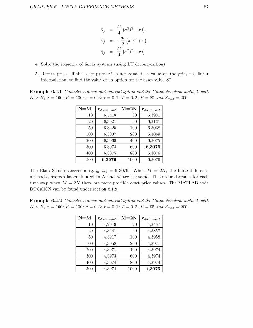
CHAPTER 6. FINITE DIFFERENCE METHODS 87
αj =δt
4
(
σ2j2 − rj)
,
βj = −δt
2
(
σ2j2 + r)
,
γj =δt
4
(
σ2j2 + rj)
.
4. Solve the sequence of linear systems (using LU decomposition).
5. Return price. If the asset price S∗ is not equal to a value on the grid, use linear
interpolation, to find the value of an option for the asset value S∗.
Example 6.4.1 Consider a down-and-out call option and the Crank-Nicolson method, with
K > B; S = 100; K = 100; σ = 0, 3; r = 0, 1; T = 0, 2; B = 85 and Smax = 200.
N=M cdown−out M=2N cdown−out
10 6,5418 20 6,3931
20 6,3921 40 6,3131
50 6,3225 100 6,3038
100 6,3037 200 6,3069
200 6,3069 400 6,3075
300 6,3074 600 6,3076
400 6,3075 800 6,3076
500 6,3076 1000 6,3076
The Black-Scholes answer is cdown−out = 6, 3076. When M = 2N , the finite difference
method converges faster than when N and M are the same. This occurs because for each
time step when M = 2N there are more possible asset price values. The MATLAB code
DOCallCN can be found under section 8.1.8.
Example 6.4.2 Consider a down-and-out call option and the Crank-Nicolson method, with
K > B; S = 100; K = 100; σ = 0, 3; r = 0, 1; T = 0, 2; B = 95 and Smax = 200.
N=M cdown−out M=2N cdown−out
10 4,2919 20 4,3457
20 4,3441 40 4,3857
50 4,3917 100 4,3958
100 4,3958 200 4,3971
200 4,3971 400 4,3974
300 4,3973 600 4,3974
400 4,3974 800 4,3974
500 4,3974 1000 4,3975

CHAPTER 6. FINITE DIFFERENCE METHODS 88
The Black-Scholes answer is cdown−out = 4, 3975. Once again, when M = 2N , the finite
difference method converges faster than when N and M are the same.
Note that in this case, when the barrier is close to the strike price, that the Crank-Nicolson
finite difference method gives more accurate results in less time steps than the lattice meth-
ods in section 4.3.7.
The MATLAB code DOCallCN can be found under section 8.1.8.
Example 6.4.3 Consider a down-and-out call option and the Crank-Nicolson method, with
K > B; S = 10; K = 9; σ = 0, 25; r = 0, 05; T = 1; B = 5 and Smax = 40.
The Black-Scholes answer is cdown−out = 1, 8141.
N=M cdown−out M=2N cdown−out
10 1,9060 20 1,8380
20 1,8379 40 1,8248
50 1,8164 100 1,8157
100 1,8157 200 1,8143
200 1,8143 400 1,8141
300 1,8141 600 1,8141
400 1,8141 800 1,8141
500 1,8141 1000 1,8141
Chapter 7
Conclusion
Pricing barrier options with numerical methods can be difficult and certain methods can
be slow to converge. This necessitates a thorough literature study to investigate the cur-
rent available pricing techniques, after which MATLAB code was implemented in order to
experiment with numerical data.
The standard binomial and trinomial methods converge extremely slow and with a non-
monotonic convergence, as one can see in section 4.3.7. Thus, adaptive barrier methods
were researched and implemented, such as the revised binomial model, the stretch tech-
nique and the interpolation technique. The interpolation technique differed in that the
convergence seemed to be monotonic while the other adaptive barrier methods had non-
monotonic convergence. The stretch technique gives the most accurate answers for a given
time step. The stretch technique was consequently adapted to find the price of discrete
barrier options, and obtained good results.
The Monte Carlo methods are easy to code though it can be slow, since tens of thousands
of simulations are needed to get an accurate answer (Wilmott 2007, 387). The conclusion
is that a variance reduction technique; the antithetic variable technique, has given more
accurate answers in comparison to the standard Monte Carlo simulation. The technique
shrinks the confidence intervals, that contains the price. However, twice as many evalua-
tions of the exponential and square root functions are required (Higham 2004, 218), hence
more computational effort is needed for a reasonable accurate answer.
The finite difference method, where the prices of barrier options on a grid (different un-
derlying share prices and time intervals) can be calculated, was also studied. It is easy
to implement and program the explicit finite difference method. However, the method
is unstable if the ratio δt/(δS)2 ≤ 1/2 is not met, and the method is slow to converge
(Wilmott 2007, 918) (Higham 2004, 294). The implicit method is stable, and results can
89
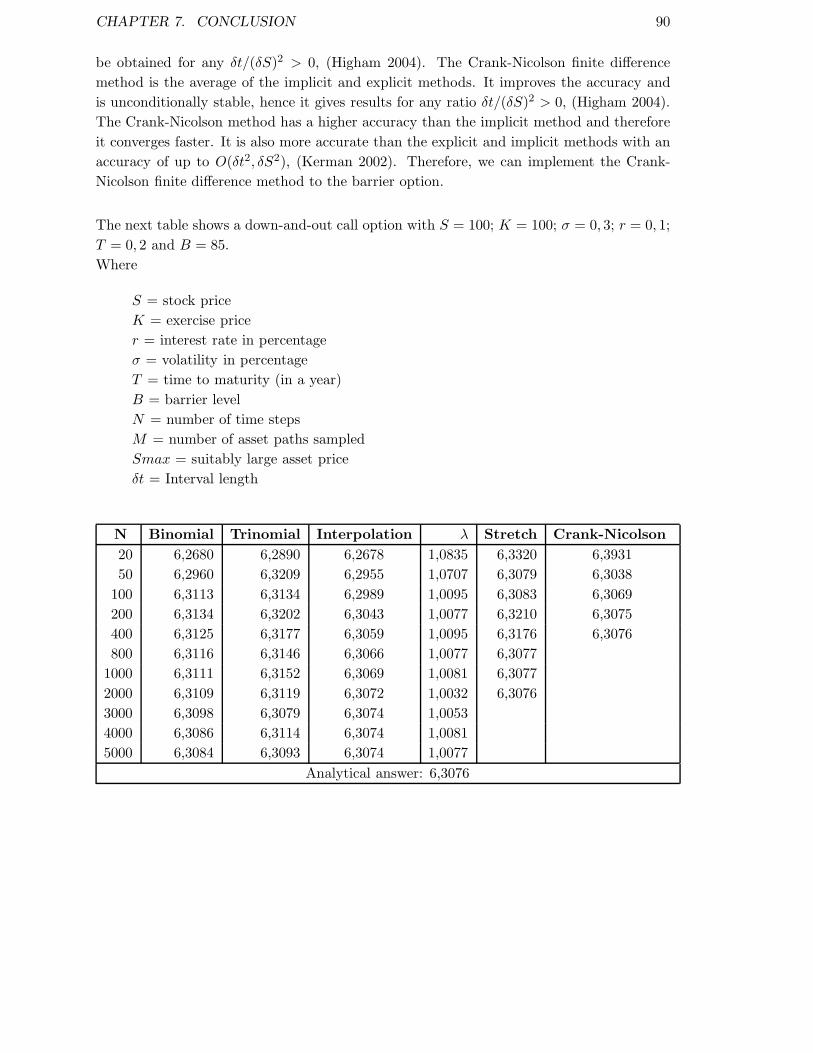
CHAPTER 7. CONCLUSION 90
be obtained for any δt/(δS)2 > 0, (Higham 2004). The Crank-Nicolson finite difference
method is the average of the implicit and explicit methods. It improves the accuracy and
is unconditionally stable, hence it gives results for any ratio δt/(δS)2 > 0, (Higham 2004).
The Crank-Nicolson method has a higher accuracy than the implicit method and therefore
it converges faster. It is also more accurate than the explicit and implicit methods with an
accuracy of up to O(δt2, δS2), (Kerman 2002). Therefore, we can implement the Crank-
Nicolson finite difference method to the barrier option.
The next table shows a down-and-out call option with S = 100; K = 100; σ = 0, 3; r = 0, 1;
T = 0, 2 and B = 85.
Where
S = stock price
K = exercise price
r = interest rate in percentage
σ = volatility in percentage
T = time to maturity (in a year)
B = barrier level
N = number of time steps
M = number of asset paths sampled
Smax = suitably large asset price
δt = Interval length
N Binomial Trinomial Interpolation λ Stretch Crank-Nicolson
20 6,2680 6,2890 6,2678 1,0835 6,3320 6,3931
50 6,2960 6,3209 6,2955 1,0707 6,3079 6,3038
100 6,3113 6,3134 6,2989 1,0095 6,3083 6,3069
200 6,3134 6,3202 6,3043 1,0077 6,3210 6,3075
400 6,3125 6,3177 6,3059 1,0095 6,3176 6,3076
800 6,3116 6,3146 6,3066 1,0077 6,3077
1000 6,3111 6,3152 6,3069 1,0081 6,3077
2000 6,3109 6,3119 6,3072 1,0032 6,3076
3000 6,3098 6,3079 6,3074 1,0053
4000 6,3086 6,3114 6,3074 1,0081
5000 6,3084 6,3093 6,3074 1,0077
Analytical answer: 6,3076

CHAPTER 7. CONCLUSION 91
∆t = 10−5
M cdown−and−out CI Time (seconds)
Monte Carlo Simulation
102 7,7065 5,7045; 9,7084 0,085
103 6,5526 5,9814; 7,1238 0,607
104 6,4942 6,3128; 6,6757 5,854
105 6,3300 6,2735; 6,3864 59,329
Antithetic Variable Technique
102 6,8957 5,9602; 7,8311 0,168
103 6,2186 5,9422; 6,4948 1,146
104 6,3099 6,2185; 6,4013 10,311
105 6,3228 6,2942; 6,3515 97,908
Analytical answer: 6, 3076
As revealed by the experimental data, Monte Carlo simulation and even the variance reduc-
tion technique, take too long. The Crank-Nicolson finite difference method for the down
and out call option gives an accurate value of the option in fewer time steps when compared
to the other numerical methods.
This dissertation offers a discussion of the theoretical background of different barrier op-
tions, an investigation of numerical techniques to determine the value of a barrier option, a
description of the algorithms and shows the implementation of the algorithms in MATLAB
code. The results are compared with the analytical solutions and results obtained in the
literature. Comments are offered on the number of subintervals needed for a valid price,
using the different numerical methods. The best lattice method is the adaptation of the
trinomial method using the stretch technique. The Monte Carlo method converges very
slowly to obtain an accurate value, whilst the Crank-Nicolson finite difference method takes
the least number of time steps to obtain an accurate value.
Further research could focus on the finite difference methods and adaptation of the finite
difference methods to price more exotic barrier options and discrete barrier options.
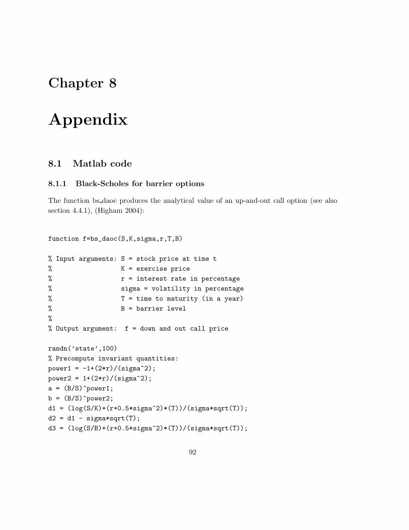
Chapter 8
Appendix
8.1 Matlab code
8.1.1 Black-Scholes for barrier options
The function bs daoc produces the analytical value of an up-and-out call option (see also
section 4.4.1), (Higham 2004):
function f=bs_daoc(S,K,sigma,r,T,B)
% Input arguments: S = stock price at time t
% K = exercise price
% r = interest rate in percentage
% sigma = volatility in percentage
% T = time to maturity (in a year)
% B = barrier level
%
% Output argument: f = down and out call price
randn(’state’,100)
% Precompute invariant quantities:
power1 = -1+(2*r)/(sigma^2);
power2 = 1+(2*r)/(sigma^2);
a = (B/S)^power1;
b = (B/S)^power2;
d1 = (log(S/K)+(r+0.5*sigma^2)*(T))/(sigma*sqrt(T));
d2 = d1 - sigma*sqrt(T);
d3 = (log(S/B)+(r+0.5*sigma^2)*(T))/(sigma*sqrt(T));
92

CHAPTER 8. APPENDIX 93
d4 = (log(S/B)+(r-0.5*sigma^2)*(T))/(sigma*sqrt(T));
d5 = (log(S/B)-(r-0.5*sigma^2)*(T))/(sigma*sqrt(T));
d6 = (log(S/B)-(r+0.5*sigma^2)*(T))/(sigma*sqrt(T));
d7 = (log(S*K/(B^2))-(r-0.5*sigma^2)*(T))/(sigma*sqrt(T));
d8 = (log(S*K/(B^2))-(r+0.5*sigma^2)*(T))/(sigma*sqrt(T));
% Normal distributions of d values:
Nd1 = 0.5*(1+erf(d1/sqrt(2)));
Nd2 = 0.5*(1+erf(d2/sqrt(2)));
Nd3 = 0.5*(1+erf(d3/sqrt(2)));
Nd4 = 0.5*(1+erf(d4/sqrt(2)));
Nd5 = 0.5*(1+erf(d5/sqrt(2)));
Nd6 = 0.5*(1+erf(d6/sqrt(2)));
Nd7 = 0.5*(1+erf(d7/sqrt(2)));
Nd8 = 0.5*(1+erf(d8/sqrt(2)));
% For down-and-out call:
if K > B
bs_daoc = S*(Nd1-b*(1-Nd8))-K*exp(-r*T)*(Nd2-a*(1-Nd7))
else
bs_daoc = S*(Nd3-b*(1-Nd6))-K*exp(-r*T)*(Nd4-a*(1-Nd5))
end
f=bs_daoc;
8.1.2 Standard options
8.1.2.1 Binomial method
The function Call bm makes use of CRR’s (section 4.1) parameters for u, d and p, and
produces the value of a European call option using a binomial lattice (see also section 4.1),
(Brandimarte 2006):
function price = Call_bm(S,K,sigma,r,T,N)
% Input arguments: S = stock price at time t
% K = exercise price
% r = interest rate in percentage
% sigma = volatility in percentage
% T = time to maturity (in a year)
% N = number of time steps
%
% Output argument: f = call price
CHAPTER 8. APPENDIX 94
% Precompute invariant quantities:
deltaT = T/N;
u = exp(sigma * sqrt (deltaT));
d = 1/u;
p = (exp(r*deltaT) - d)/(u-d);
discount = exp(-r*deltaT);
p_u = discount*p;
p_d = discount*(1-p);
% Set up S values:
SVals = zeros(2*N+1,1);
SVals(1) = S*d^N;
for i = 2:2*N+1
SVals(i) = u*SVals(i-1);
end
% Set up terminal CALL values:
CVals = zeros (2*N+1,1);
for i = 1:2:2*N+1
CVals(i) = max(SVals(i)-K,0);
end
% Work backwards:
for tau = 1 : N
for i = (tau+1):2: (2*N+1-tau)
CVals(i) = p_u*CVals(i+1) + p_d*CVals(i-1);
end
end
f = CVals(N+1);
The function Call bmh makes use of (Higham 2004) parameters for u, d and p, and produces
the value of a European call option using a binomial lattice, the program is almost identical
to the program above but with:
u=exp(sigma*sqrt(dt)+(r-0.5*sigma^2)*dt);
d=exp(-sigma*sqrt(dt)+(r-0.5*sigma^2)*dt);
p=0.5;
8.1.2.2 Accuracy of option value
The function newtest bm returns the value of a European call option and the number of
time steps using a binomial lattice (see also section 4.1.1):
function value=newtest_bm(S,K,sigma,r,T,tol)

CHAPTER 8. APPENDIX 95
% Input arguments: S = asset price at time t
% K = exercise price
% r = interest rate in percentage
% sigma = volatitly in percentage
% T = time to maturity (in a year)
% B = barrier level
% tol = tolerance
%
% Output arguments: f = call price
% N = number of time steps
%
% Precompute invariant quantities:
f0=0;
for N = 1:5000
deltaT = T/N;
u = exp(sigma * sqrt (deltaT));
d = 1/u;
p = (exp(r*deltaT) - d)/(u-d);
discount = exp(-r*deltaT);
p_u = discount*p;
p_d = discount*(1-p);
% Set up S values:
SVals = zeros(2*N+1,1);
SVals(1) = S*d^N;
for i = 2:2*N+1
SVals(i) = u*SVals(i-1);
end
% Set up terminal CALL values:
CVals = zeros (2*N+1,1);
for i = 1:2:2*N+1
CVals(i) = max(SVals(i)-K,0);
end
% Work backwards:
for tau = 1 : N
for i = (tau+1):2: (2*N+1-tau)
CVals(i) = p_u*CVals(i+1) + p_d*CVals(i-1);
end

CHAPTER 8. APPENDIX 96
end
f = CVals(N+1);
%Apply tolerance difference
if abs(f-f0) < tol
break
end
f0 = f;
end
value=f;
display(value);
display(f0);
display(N);
end
8.1.2.3 Trinomial method
The function Call tm returns the value of a European call option using a trinomial lattice
(see also section 4.2), (Brandimarte 2006):
function f=Call_tm(S,K,sigma,r,T,N)
% Input arguments: S = stock price at time t
% K = exercise price
% r = interest rate in percentage
% sigma = volatility in percentage
% T = time to maturity (in a year)
% N = number of time steps
%
% Output argument: f = call price
% Precompute invariant quantities:
dt =T/N;
dx = sigma*sqrt(2*dt);
discount = exp(-r*dt) ;
pu = (((exp((r*dt)/2)-exp(-sigma*sqrt(dt/2))) ...
/(exp(sigma*sqrt(dt/2))- exp(-sigma*sqrt(dt/2))))^2);
pd = (((exp(sigma*sqrt(dt/2))-exp((r*dt)/2)) ...
/(exp(sigma*sqrt(dt/2))-exp(-sigma*sqrt(dt/2))))^2);
pm = 1 - pu -pd;
p_u = discount*pu;
p_d = discount*pd;
CHAPTER 8. APPENDIX 97
p_m = discount*pm;
% Set up S values:
Stree = zeros(2*N+1,1);
Stree(1) = S*exp(-N*dx);
exp_dx = exp(dx);
for j = 2:2*N+1
Stree(j) = exp_dx*Stree(j-1);
end
% Set up terminal CALL values:
OptValues = zeros(2*N+1,2);
x = mod(N,2)+1;
for j = 1:2*N+1
OptValues(j,x) = max(Stree(j)-K,0);
end
% Work backwards:
for x = N-1:-1:0;
know = mod(x,2)+1;
knext = mod(x+1,2)+1;
for j = N-x+1:N+x+1
OptValues(j,know) = p_d*OptValues(j-1,knext)+p_m*...
OptValues(j,knext)+ p_u*OptValues(j+1,knext);
end
end
f = OptValues(N+1,1);
8.1.3 Barrier options
8.1.3.1 Binomial method
The function KOCall bm makes use of CRR’s (section 4.1) parameters for u, d and p, and
returns the value of a up-and-out European call option using a binomial lattice (see also
section 4.3), (Brandimarte 2006):
function f=KOCall_bm(S,K,sigma,r,T,N,B)
% Input arguments: S = stock price at time t
% K = exercise price
% r = interest rate in percentage
% sigma = volatility in percentage
CHAPTER 8. APPENDIX 98
% T = time to maturity (in a year)
% B = barrier level
% N = number of time steps
%
% Output argument: f = down and out call price
% Precompute invariant quantities:
deltaT = T/N;
u = exp(sigma * sqrt (deltaT)) ;
d = 1/u;
p = (exp(r*deltaT) - d)/(u-d) ;
discount = exp(-r*deltaT);
p_u = discount*p;
p_d = discount*(1-p);
% set up S values
SVals = zeros(2*N+1,1) ;
SVals(1) = S*d^N;
for i = 2:2*N+1
SVals(i) = u*SVals(i-1);
end
% set up terminal CALL values
CVals = zeros (2*N+1,1);
for i = 1:2:2*N+1
if SVals(i) <= B
CVals(i) = 0;
else
CVals(i) = max(SVals(i)-K,0) ;
end
end
% work backwards
for tau = 1 : N
for i = (tau+1):2: (2*N+1-tau)
if SVals(i) <= B
CVals(i) = 0;
else
CVals(i) = p_u*CVals(i+1) + p_d*CVals(i-1) ;
end
end
CHAPTER 8. APPENDIX 99
end
f = CVals(N+1);
disp(N)
disp(f)
Notes:
The function KOCall bmh makes use of (Higham 2004) parameters for u, d and p, and
produces the value of a European call option using a binomial lattice, the program is almost
identical to the program above, but with:
u=exp(sigma*sqrt(dt)+(r-0.5*sigma^2)*dt);
d=exp(-sigma*sqrt(dt)+(r-0.5*sigma^2)*dt);
p=0.5;
8.1.3.2 Trinomial method
The function KOCall tm returns the value of a down-and-out European call option using a
trinomial lattice (see also section 4.3), (Brandimarte 2006):
function f = KOCall_tm(S,K,sigma,r,T,n,B)
% Input arguments: S = stock price at time t
% K = exercise price
% r = interest rate in percentage
% sigma = volatility in percentage
% T = time to maturity (in a year)
% B = barrier level
% N = number of time steps
%
% Output argument: f = down and out call price
% Precompute invariant quantities:
dt = T/N;
dx = sigma*sqrt(2*dt);
discount = exp(-r*dt) ;
pu = (((exp((r*dt)/2)-exp(-sigma*sqrt(dt/2))) ...
/(exp(sigma*sqrt(dt/2))- exp(-sigma*sqrt(dt/2))))^2);
pd = (((exp(sigma*sqrt(dt/2))-exp((r*dt)/2)) ...
/(exp(sigma*sqrt(dt/2))-exp(-sigma*sqrt(dt/2))))^2);
pm = 1 - pu -pd;
p_u = discount*pu;

CHAPTER 8. APPENDIX 100
p_d = discount*pd;
p_m = discount*pm;
% Set up S values:
Stree = zeros(2*N+1,1);
Stree(1) = S*exp(-N*dx);
exp_dx = exp(dx);
for j = 2:2*N+1
Stree(j) = exp_dx*Stree(j-1);
end
% Set up terminal CALL values:
OptValues = zeros(2*N+1,2);
x = mod(N,2)+1;
for j = 1:2*N+1
if Stree(j,x) <= B
OptValues(j,x) = 0;
else
OptValues(j,x) = max(Stree(j,x)-K,0);
end
end
% Work backwards:
for x = N-1:-1:0;
know = mod(x,2)+1;
knext = mod(x+1,2)+1;
for j = N-x+1:N+x+1
if Stree(j) <= B
OptValues(j,know) = 0;
else
OptValues(j,know) = p_d*OptValues(j-1,knext)+p_m*...
OptValues(j,knext)+ p_u*OptValues(j+1,knext);
end
end
end
f = OptValues(N+1,1);
Notes:
This program does not give answers for an odd number of ”N” time steps. Unlike binomial
lattices, one must store at least two consecutive time layers of the lattice, since there is no
alternation between odd- and even- indexed entries in the array. Thus, one must make use

CHAPTER 8. APPENDIX 101
of a two-column array, (Brandimarte 2006).
8.1.4 Interpolation technique
The function KOCall tm int returns the value of a down-and-out European call option using
the interpolation technique (see also section 4.3.5):
function f=KOCall_tm_int(S,K,sigma,r,T,N,B)
% Input arguments: S = stock price at time t
% K = exercise price
% r = interest rate in percentage
% sigma = volatility in percentage
% T = time to maturity (in a year)
% B = barrier level
% N = number of time steps
%
% Output argument: f = down and out call price
% Precompute invariant quantities:
dt=T/N;
dx=sigma*sqrt(2*dt);
discount = exp(-r*dt);
pu = (((exp((r*dt)/2)-exp(-sigma*sqrt(dt/2))) ...
/(exp(sigma*sqrt(dt/2))- exp(-sigma*sqrt(dt/2))))^2);
pd = (((exp(sigma*sqrt(dt/2))-exp((r*dt)/2)) ...
/(exp(sigma*sqrt(dt/2))-exp(-sigma*sqrt(dt/2))))^2);
pm= 1 - pu -pd;
p_u= discount*pu;
p_d=discount*pd;
p_m=discount*pm;
exp_dx=exp(dx);
%Calculate the stock price
Stree=zeros(2*N+1,1);
Stree(1)=S*exp(-N*dx);
for j=2:2*N+1
Stree(j)=exp_dx*Stree(j-1);
end
%Working outer barrier and inner barrier
CHAPTER 8. APPENDIX 102
t=mod(N,2)+1;
for j=1:2*N+1
if Stree(j,t) >= B
out= Stree(j,t);
break
end
end
for j=1:2*N+1
if Stree(j,t) >= out
in= Stree(j-1,t);
break
end
end
%K0Call_tm(S,K,sigma,r,T,N,outb)
%Calculate the option price with outter barrier
OptValues2=zeros(2*N+1,2);
for j=1:2*N+1
if Stree(j,t) <=out
OptValues2(j,t)=0;
else
OptValues2(j,t)=max(Stree(j,t)-K,0);
end
end
for t=N-1:-1:0;
knows= mod(t,2)+1;
knexts=mod(t+1,2)+1;
for j=N-t+1:N+t+1
if Stree(j)<=out
OptValues2(j,knows) = 0;
else
OptValues2(j,knows)=p_d*OptValues2(j-1,knexts)+p_m*...
OptValues2(j,knexts)+ p_u*OptValues2(j+1,knexts);
end
end
end
foutb=OptValues2(N+1,1);
%K0Call_tm(S,K,sigma,r,t,n,inb)
CHAPTER 8. APPENDIX 103
%Calculate the option price with inner barrier
%Calculate the stock price
Stree2=zeros(2*N+1,1);
Stree2(1)=S*exp(-N*dx);
for j=2:2*N+1
Stree2(j)=exp_dx*Stree2(j-1);
end
t=mod(N,2)+1;
OptValues=zeros(2*N+1,2);
for j=1:2*N+1
if Stree2(j,t) <=in
OptValues(j,t)=0;
else
OptValues(j,t)=max(Stree2(j,t)-K,0);
end
end
for t=N-1:-1:0;
knows= mod(t,2)+1;
knexts=mod(t+1,2)+1;
for j=N-t+1:N+t+1
if Stree2(j)<=in
OptValues(j,knows) = 0;
else
OptValues(j,knows)=p_d*OptValues(j-1,knexts)+p_m*...
OptValues(j,knexts)+ p_u*OptValues(j+1,knexts);
end
end
end
finb=OptValues(N+1,1);
%Interpolate
f=finb +(B-in)*((foutb - finb)/(out - in));
display(f)
display(in)
display(out)
8.1.5 Stretch technique
The function stretch tm returns the value of a down-and-out European call option using
the stretch technique (see also section 4.3.6):

CHAPTER 8. APPENDIX 104
function f = stretch_tm(S,K,r,sigma,T,N,B)
% Input arguments: S = stock price at time t
% K = exercise price
% r = interest rate in percentage
% sigma = volatility in percentage
% T = time to maturity (in a year)
% B = barrier level
% N = number of time steps
%
% Output argument: f = down and out call price
dt= T/N;
%Work out lamda (nn)
n=(log(S/B))/(sigma*sqrt(dt));
if n> 2
nn= n/floor(n);
else
nn=n;
end
display(nn)
% Precompute invariant quantities:
dx=nn*sigma*sqrt(dt);
discount = exp(-r*dt);
u=r-((sigma^2)/2);
pu = (1/(2*nn^2))+((u*sqrt(dt))/(2*nn*sigma));
pd = (1/(2*nn^2))-((u*sqrt(dt))/(2*nn*sigma));
pm= 1 - 1/(nn^2);
p_u= discount*pu;
p_d=discount*pd;
p_m=discount*pm;
%Work out stock price
Stree=zeros(2*N+1,1);
Stree(1)=S*exp(-N*dx);
exp_dx=exp(dx);
for j=2:2*N+1
Stree(j)=exp_dx*Stree(j-1);
end
%Work out option price
OptValues=zeros(2*N+1,2);

CHAPTER 8. APPENDIX 105
t=mod(N,2)+1;
for j=1:2*N+1
if Stree(j,t) <=B
OptValues(j,t)=0;
else
OptValues(j,t)=max(Stree(j,t)-K,0);
end
end
for t=N-1:-1:0;
know= mod(t,2)+1;
knext=mod(t+1,2)+1;
for j=N-t+1:N+t+1
if Stree(j)<=B
OptValues(j,know) = 0;
else
OptValues(j,know)=p_d*OptValues(j-1,knext)+p_m*...
OptValues(j,knext)+ p_u*OptValues(j+1,knext);
end
end
end
f=OptValues(N+1,1);
8.1.6 Monte Carlo method
The function monte returns the value of a down-and-out European call option using a Monte
Carlo simulation (Higham 2004, 200) (see also section 5.2):
function conf=monte(S,K,sigma,r,T,Dt,N,M)
% Input arguments: S = stock price at time t
% K = exercise price
% r = interest rate in percentage
% sigma = volatility in percentage
% T = time to maturity (in a year)
% B = barrier level
% N = number of time steps
% Dt = Interval length
% M = number of asset paths sampled
%
% Output argument: conf = confidence interval
%Monte Carlo for a knock out call option
CHAPTER 8. APPENDIX 106
%Smax<B for an up-and-out call option
%Smax>B for an up-and-out call option
%state uses Matlabs Marsaglias ziggurat algorithm so generate numbers and creating
%an 100x100 matrix
randn(’state’,100)
Dt=N/T;
f=zeros(M,1);
for i= 1:M
Sfinal = S*cumprod(exp((r-0.5*sigma^2)*Dt+sigma*sqrt(Dt)*randn(N,1)));
Smax=max(Sfinal);
if Smax>B
f(i) = exp(-r*T)*max(Sfinal(end)-K,0);
end
end
xM = mean(f);
yM = std(f);
conf = [xM - 1.96*yM/sqrt(M), xM + 1.96*yM/sqrt(M)];
disp(xM)
disp(conf)
8.1.7 Antithetic variable technique
The function monte anti returns the value of a down-and-out European call option using
the antithetic variable technique (Higham 2004, 226) (see also section 5.3):
function conf=monte_anti(S,K,sigma,r,T,Dt,M,B)
%Monte Carlo for a out call option
% < up and > down
% Input arguments: S = stock price at time t
% K = exercise price
% r = interest rate in percentage
% sigma = volatility in percentage
% T = time to maturity (in a year)
% B = barrier level
% N = number of time steps
% Dt = Interval length
% M = number of asset paths sampled
%

CHAPTER 8. APPENDIX 107
% Output argument: conf = confidence interval
randn(’state’,100)
N=T/Dt;
f=zeros(M,1);
fanti=zeros(M,1);
for i= 1:M
samples = randn(N,1);
% standard Monte Carlo
Sfinal = S*cumprod(exp((r-0.5*sigma^2)*Dt+sigma*sqrt(Dt)*samples));
Smax=max(Sfinal);
if Smax>B
f(i) = exp(-r*T)*max(Sfinal(end)-K,0);
end
% antithetic path
Sfinal2 = S*cumprod(exp((r-0.5*sigma^2)*Dt-sigma*sqrt(Dt)*samples));
Smax2=max(Sfinal2);
f2=0;
if Smax2>B
f2 = exp(-r*T)*max(Sfinal2(end)-K,0);
end
fanti(i)=0.5*(f(i)+f2);
end
xM = mean(f);
yM = std(f);
conf = [xM - 1.96*yM/sqrt(M), xM + 1.96*yM/sqrt(M)];
xManti = mean(fanti);
yManti = std(fanti);
confanti = [xManti - 1.96*yManti/sqrt(M), xManti + 1.96*yManti/sqrt(M)];
disp(xManti)
disp(confanti)
8.1.8 Crank-Nicolson method
The function DOCallCN (Brandimarte 2006, 487) returns the value of a down-and-out
European call option using the Crank-Nicolson method (see also section 6.4):
CHAPTER 8. APPENDIX 108
function f = DOCallCN(S,K,r,T,sigma,B,Smax,N,M)
% Input arguments: S = stock price at time t
% K = exercise price
% r = interest rate in percentage
% sigma = volatility in percentage
% T = time to maturity (in a year)
% B = barrier level
% N = number of time steps
% M = number of asset paths sampled
% Smax = suitably large asset price
%
% Output argument: f = down and out call price
%set up grid
dt = T/N;
dS = (Smax - B)/M;
matval = zeros(M+1,N+1);
vetS = linspace(B,Smax,M+1)’;
vetj = vetS/dS;
%set up boundary conditions
matval(:,N+1) = max(vetS-K,0);
matval(1,:) = 0;
matval(M+1,:) = Smax;
%set up coefficients
alpha = 0.25 * dt * (sigma^2*(vetj.^2) -r*vetj);
beta = - dt * 0.5 * (sigma^2*(vetj.^2) + r);
gamma = 0.25 * dt * (sigma^2*(vetj.^2) +r*vetj);
C = -diag(alpha(3:M) ,-1) + diag(1-beta(2:M)) - diag(gamma(2:M-1) ,1) ;
[L,U] = lu(C);
D = diag(alpha(3:M) ,-1) + diag(1+beta(2:M)) + diag(gamma(2:M-1) ,1) ;
%solve the sequence of linear systems
for i = N : -1: 1
matval(2:M,i) = U\(L\(D*matval(2:M,i+1)));
end
%return price, possibly by linear interpolation outside the grid
f = interp1(vetS,matval(:,1),S);

Bibliography
Ahn, D., Figlewski, S. and Gao, B. 1999. Pricing discrete barrier options with an adaptive
mesh model, Journal of Derivatives 6(4): 33–43.
Bjork, T. 2009. Arbitrage theory in continuous time, 3rd ed, Oxford University Press, New
York.
Boyle, P. and Lau, S. 1994. Bumping up against the barrier, The journal of derivatives
1(4): 6–14.
Brandimarte, P. 2006. Numerical Methods in Finance and Economics: A MATLAB-Based
Introduction, 2nd ed, John Wiley & Sons, Hoboken, NJ.
Broadie, M., Glasserman, P. and Kou, S. 1997. A continuity correction for discrete barrier
options, Mathematical finance 7(4): 325–348.
Broadie, M., Glasserman, P. and Kou, S. 1999. Connecting discrete and continuous path-
dependent options, Finance and stochastics 3(1): 55–82.
Cheney, W. and Kincaid, D. 2004. Numerical Mathematics and Computing, 5th ed, Thom-
son, Brooks/Cole, USA.
Chriss, N. 1997. Black-Scholes and Beyond Option Pricing Models, McGraw-Hill, New
York.
Cox, J., Ross, S. and Rubinstein, M. 1979. Option pricing: A simplified approach, Journal
of financial economics September(1): 1–35.
De Klerk, J. 2009. Partial differential equations (numerical), Study notes for the model
TGWS312, NWU.
Derman, E., Kani, I., Ergener, D. and Bardhan, B. 1995. Enhanced Numerical Methods for
Options with Barriers, Goldman Sachs & Co, New York.
Dewynne, J., Howison, S. and Wilmott, P. 1995. The mathematics of financial derivatives:
A student introduction, Press Syndicate of the University of Cambridge, Cambridge,
UK.
109

BIBLIOGRAPHY 110
Forsyth, P., Vetzal, K. and Zvan, R. 2000. PDE methods for pricing barrier options, Journal
of economic dynamics and control 24(1): 1563–1590.
Haug, E. 1998. Complete Guide to Option Pricing Formulas, 2nd ed, McGraw Hill, New
York.
Higham, D. J. 2004. An Introduction to Financial Option Valuation: Mathematics, Stochas-
tics and Computation, Cambridge University Press, New York.
Horfelt, P. 2003. Extension of the corrected barrier approximation by Broadie, Glasserman,
and Kou, Finance and Stochastic 7(1): 231–243.
Hull, J. 2000. Options, futures and other derivatives, 4th ed, Pearson Education, Upper
saddle river, NJ.
Kamrad, B. and Ritchken, P. 1991. Multinomial approximaing models for options with k
state variables, Management Science 37(12): 1640–1652.
Kerman, J. 2002. Numerical Methods for Option Pricing: Binomial and Finite Difference
Approximations, Thesis, www.stat.columbia.edu/ kerman.
Kotze, A. 1999. Financial Chaos Theory: Barrier options traded in the South African
markets, Financial Chaos Theory, Doornfontein, SA.
Luenberger, D. 1998. Investment Science, Oxford University press, New York.
Merton, R. 1973. The theory of rational option pricing, Bell J. of Economics and Manage-
ment Science 4(1): 141–183.
Neftci, S. 2008. Principles of Financial Engineering, 2nd ed, Elsevier, California, USA.
Reiner, E. and Rubinstein, M. 1991. Breaking down the barriers, Risk 4(8): 28–35.
Ritchken, P. 1995. On pricing barrier options, Journal of derivatives 3(2): 19–28.
Roman, S. 2004. Introduction to the Mathematics of Finance from Risk Manangement to
Options Pricing, Springer, New York, USA.
Wilmott, P. 2007. Paul Wilmott introduces quantitative finance, 2nd ed, John Wiley & Sons,
London, UK.