numerical methods for derivative pricing with … methods for derivative pricing with applications...
TRANSCRIPT
Numerical Methods ForDerivative Pricing with
Applications to Barrier Options
by
Kavin Sin
Supervisor: Professor Lilia Krivodonova
A thesispresented to the University of Waterloo
in fulfillment of thethesis requirement for the degree of
Master of Sciencein
Computational Mathematics
Waterloo, Ontario, Canada, 2010
c© Kavin Sin 2010

I hereby declare that I am the sole author of this thesis. This is a truecopy of the thesis, including any required final revisions, as accepted by myexaminers.
I understand that my thesis may be made electronically available to thepublic.
ii
Abstract
In this paper, we study the use of numerical methods to price barrier options.
A barrier option is similar to a vanilla option with one exception. If the option
ceases to exist then the payoff is zero. If the stock price hits the pre-agreed
upon barrier price, then the option ceases to exist or comes into existent
depending on the type of a barrier option i.e. knock in or knock out. The
immediate payoff is either the same as for a vanilla call or zero, respectively.
We apply a number of classical and recently proposed numerical techniques to
approximate the solutions of the Black-Scholes and Heston models. Our main
goal is to use the more complicated and accurate Heston model. The Black-
Scholes equation is used as a verification tool. Our two major approaches are
Monte Carlo simulations and a finite difference method. The Heston model
relies on five parameters that characterize the current market behavior. We
approximate these from market data by calibrating the model using the least
square technique and Levenberg-Marquardt method. We present the results
of our simulations and discuss our findings. MATLAB codes required to
implement the models are provided in the appendix.
iii

Acknowledgements
I would like to take this opportunity to thank Professor Lilia Krivodonova
for her help and advice throughout my research period. I would also like to
thank Andree Susanto for his help with LATEX. I also would like to show my
gratitude to Professor Li Yuying for an amazing numerical method class that
helped me learn and challenge my thinking thus, enabling me to finish my
thesis.
iv
Contents
List of Figures vii
1 Introduction 1
2 Barrier Options 3
2.1 Knock Out Options . . . . . . . . . . . . . . . . . . . . . . . . 4
2.1.1 Up and out call: . . . . . . . . . . . . . . . . . . . . . . 4
2.1.2 Down and out call: . . . . . . . . . . . . . . . . . . . . 4
2.2 Knock In Options . . . . . . . . . . . . . . . . . . . . . . . . . 5
2.2.1 Up and in call: . . . . . . . . . . . . . . . . . . . . . . 5
2.2.2 Down and in call: . . . . . . . . . . . . . . . . . . . . . 5
3 Monte Carlo Simulations On Black-Scholes Model 7
3.1 Generating Stock Paths . . . . . . . . . . . . . . . . . . . . . 7
4 Stochastic Volatility Model 12
4.1 Milstein Method . . . . . . . . . . . . . . . . . . . . . . . . . 13
4.1.1 Generation of Correlated Random Samples φ(1) φ(2) . . 15
4.1.2 Covariance Matrices . . . . . . . . . . . . . . . . . . . 16
4.2 Quadratic Exponential Method (QE) . . . . . . . . . . . . . . 23
4.2.1 Sampling The Underlying Stock Price . . . . . . . . . . 25
v
5 Model Calibration 30
5.1 Levenberg-Marquardt (LM) method . . . . . . . . . . . . . . . 31
5.1.1 Matlab Function lsqnonlin . . . . . . . . . . . . . . . . 33
6 Numerical Solution of Option Pricing Using Finite Difference
Method 36
6.1 Heston PDE . . . . . . . . . . . . . . . . . . . . . . . . . . . . 36
6.1.1 Setting Up Non Uniform Grid . . . . . . . . . . . . . . 37
6.1.2 Finite Difference Scheme . . . . . . . . . . . . . . . . . 39
6.1.3 ADI Scheme . . . . . . . . . . . . . . . . . . . . . . . . 40
vi
List of Figures
3.1 Comparison of the error with MC and improved MC method. . . . . . . 11
4.1 Comparison between Milstein MC and exact option price with N=100
time steps and number of simulations M=1000000 . . . . . . . . . . . 19
4.2 Shows the comparison between Milstein’s MC and exact option price with
time step N=1000 and Number of simulation M=1000000 . . . . . . . . 20
5.1 May 2010 market implied volatilities for liquid options obtained from
Bloomberg Professional. . . . . . . . . . . . . . . . . . . . . . . . 34
6.1 Two dimensional grid for S and V with Smax=220, Vmax=1.1, and K=55. 39
6.2 DIC option price functions U given by Table 12. . . . . . . . . . . . . 43
6.3 DOC option price functions U given by Table 12. . . . . . . . . . . . 44
vii
Chapter 1
Introduction
The most important formula for pricing vanilla options in financial math-
ematic is the Black-Scholes (BS) equation [3]. Black-Scholes model has a
closed form formula and can be used to price European vanilla put and call
options. Because of its simplicity, the BS model is widely used by banks
and other financial institutions. The model assumes that the price of heavily
traded assets follow a geometric Brownian motion with constant drift and
volatility. However, there are well known flaws with these assumptions. One
of the problems is that volatility in fact behaves in a random manner. Heston
model is one of the most well known stochastic volatility models that we can
used to address this problem. The model was proposed by Heston in 1993
[8] as an extension the Black-Scholes model. Unlike the BS model, the Hes-
ton takes into account the non log-normal distribution of asset returns and
non constant volatility. Implied volatility surfaces generated by the Heston
model look like the empirical implied volatility surfaces. One drawback of
the Heston model is that it does not have a closed formula for any options
other than vanilla options. However, some numerical methods such as Monte
Carlo simulations and finite difference methods were proposed to deal with
this problem.
1

In this paper, we use numerical methods to compute down and out barrier
options using both BS and Heston models. First, we consider the simpler BS
model. We compute down and out barrier option using standard Monte Carlo
method. Then, we will use improved Monte Carlo method proposed by Moon
[14] to price down and out barrier option. The exact solution will be used to
compare the error between these two methods. In chapter 4, we introduce
Heston stochastic volatility and two numerical methods (Milstein and QE)
that can be used to discretize the model. In chapter 5, model calibration is
introduced to estimate five unknown Heston’s parameters using Levenberg-
Marquardt method [12] and Matlab command ”lsqnonlin”. In Chapter 6, the
finite difference method is used to discretize the Heston partial differential
equation. Furthermore, explicit and alternating direction implicit scheme
(ADI) [10] are used to approximate vanilla options and barrier options.
2
Chapter 2
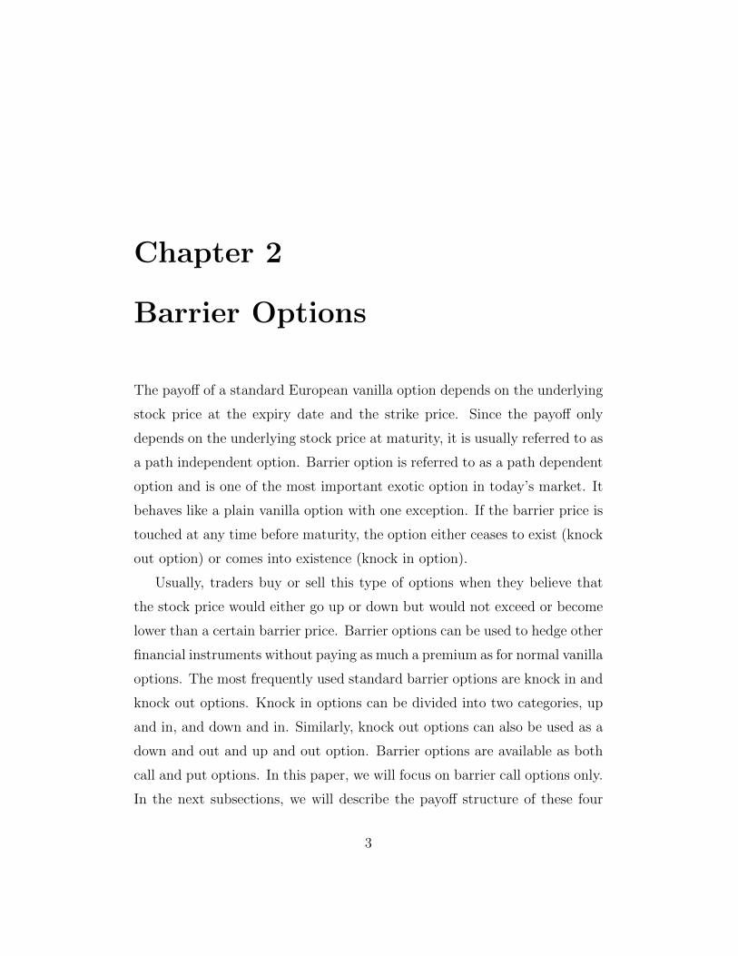
Barrier Options
The payoff of a standard European vanilla option depends on the underlying
stock price at the expiry date and the strike price. Since the payoff only
depends on the underlying stock price at maturity, it is usually referred to as
a path independent option. Barrier option is referred to as a path dependent
option and is one of the most important exotic option in today’s market. It
behaves like a plain vanilla option with one exception. If the barrier price is
touched at any time before maturity, the option either ceases to exist (knock
out option) or comes into existence (knock in option).
Usually, traders buy or sell this type of options when they believe that
the stock price would either go up or down but would not exceed or become
lower than a certain barrier price. Barrier options can be used to hedge other
financial instruments without paying as much a premium as for normal vanilla
options. The most frequently used standard barrier options are knock in and
knock out options. Knock in options can be divided into two categories, up
and in, and down and in. Similarly, knock out options can also be used as a
down and out and up and out option. Barrier options are available as both
call and put options. In this paper, we will focus on barrier call options only.
In the next subsections, we will describe the payoff structure of these four
3
types of call barrier options.
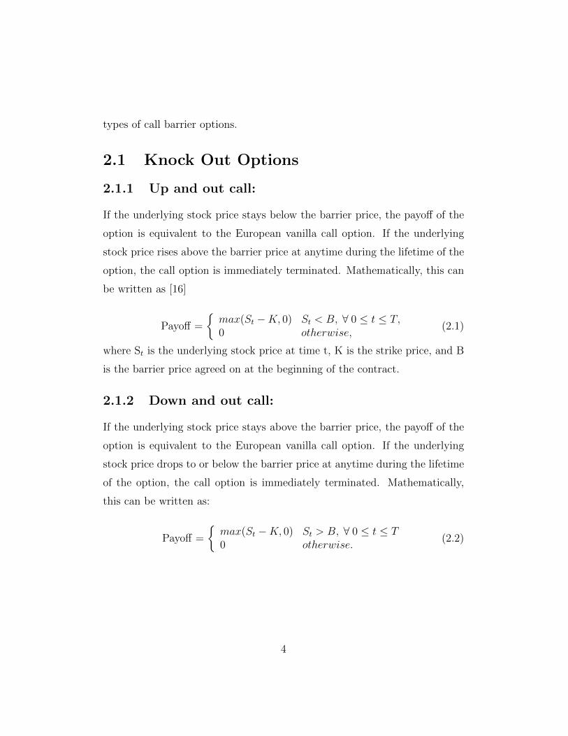
2.1 Knock Out Options
2.1.1 Up and out call:
If the underlying stock price stays below the barrier price, the payoff of the
option is equivalent to the European vanilla call option. If the underlying
stock price rises above the barrier price at anytime during the lifetime of the
option, the call option is immediately terminated. Mathematically, this can
be written as [16]
Payoff =
{max(St −K, 0) St < B, ∀ 0 ≤ t ≤ T,0 otherwise,
(2.1)
where St is the underlying stock price at time t, K is the strike price, and B
is the barrier price agreed on at the beginning of the contract.
2.1.2 Down and out call:
If the underlying stock price stays above the barrier price, the payoff of the
option is equivalent to the European vanilla call option. If the underlying
stock price drops to or below the barrier price at anytime during the lifetime
of the option, the call option is immediately terminated. Mathematically,
this can be written as:
Payoff =
{max(St −K, 0) St > B, ∀ 0 ≤ t ≤ T0 otherwise.
(2.2)
4
2.2 Knock In Options
2.2.1 Up and in call:
If the underlying stock price rises to or above the barrier price at anytime
during the lifetime of the option, the payoff of the option is equivalent to
European vanilla call option. If the underlying stock price trades below the
barrier price, the call option is immediately terminated. Mathematically, it
can be written as
Payoff =
{0 St < B, ∀ 0 ≤ t ≤ Tmax(St −K, 0) otherwise.
(2.3)
2.2.2 Down and in call:
If the underlying stock price trades at or below the barrier price at anytime
during the lifetime of the option, the payoff of the option is equivalent to
European vanilla call option. If the option trades above the barrier price,
the call option is immediately terminated. Mathematically, it can be written
as
Payoff =
{0 St > B, ∀ 0 ≤ t ≤ Tmax(St −K, 0) otherwise.
(2.4)
Lemma:
The value of the down and out call plus down and in call option with the
same barrier price and strike price is equal the value of the vanilla call option.
Similarly, the value of the up and out call plus the up and in call option is
also equal to vanilla call option. Throughout this paper, we will use DOC
to denote down and out call option price, UOC to denote up and out call
5
option price, DIC to denote down and in call option price, UIC to denote up
and in call option price and C to denote vanilla call option. Below is a proof
of the lemma stated above.
Assuming that the expected future payoff is discounted to the present day at the risk-free rate r, then C, DOC, DIC, UOC, UIC formulas are given as
C=e−rT EQ(max(ST -K,0))
DOC=e−rT EQ(max(ST -K,0)* 1ST>B)
DIC=e−rT EQ(max(ST -K,0)* 1ST≤B)
UOC=e−rT EQ(max(ST -K,0)* 1ST<B)
UIC=e−rT EQ(max(ST -K,0)* 1ST≥B)
Summing DOC and DIC, and UOC and UIC we get
DOC+DIC=e−rT EQ(max(ST -K,0)* (1ST>B +1ST≤B) )=e−rT EQ(max(ST -K,0) )=C
UOC+UIC= e−rT EQ(max(ST -K,0)* (1ST<B +1ST≥B) )=e−rT EQ(max(ST -K,0) )=C
end of proof.
Note that the payoff for the knock out and knock in put options is similar
to the call with one exception. Instead of having the underlying stock price
minus the strike price, the knock in and knock out put options have the strike
price minus the underlying stock price.
Payoff = max(K − ST , 0)
6
Chapter 3
Monte Carlo Simulations OnBlack-Scholes Model
Monte Carlo (MC) simulations rely on risk neutral valuation. The pricing
of derivative options is given by the expected value of its discounted payoffs.
First, the technique generates pricing paths for the underlying stock via
random simulations. Then it uses these pricing paths to compute the payoffs.
Finally, payoffs are averaged and discounted back to today’s prices and these
results give the value of the option prices. In this section we will use the
classical Black-Scholes model framework and apply Monte Carlo simulations
to compute down and out option price. Note that there exists a closed
form solution for this problem, and, therefore, it is not necessary to use
simulations. However, in this paper we use MC simulations for illustrative
purposes.
3.1 Generating Stock Paths
Assume that the asset price follows a geometric Brownian motion with a
constant volatility and interest rate. Brownian motion process can be used if
we assume that the market is dominated by the normal events. This process
7
can be written as the following stochastic differential equation for the asset
return [14]
dSt = Stµdt+ StσdWt, (3.1)
where
St - stock price at time t
µ - rate of return of the underlying stock price
σ -constant volatility
Wt- Wiener process
Let us assume that the asset returns follow a log normal distribution, i.e.,
G(t) = ln(St). Applying Itos lemma we get
dG(t) =dG
StdSt +
dG
dtdt+
1
2
d2G
dS2t
dS2t ,
where
dG
dt= 0,
dG
St=
1
St,d2G
dS2t
=−1
S2t
,
d ln(St) =1
St(Strdt+ StσdWt) + 0 +
1
2
(−1)
S2t
S2t σ
2dt,
d ln(St) = (r − 1
2σ2)dt+ σdWt. (3.2)
Integrating both side from 0 to t we get
ln(St)− ln(S0) = (r − 1
2σ2)t+ σWt,
St = S0e(r− 1
2σ2)t+σWt . (3.3)
In order to generate stock paths, we discretize (3.3) as follows
St+1 = Ste(r− 1
2σ2)∆t+σ
√∆tZt ,
8
where ∆t is the time step, and Zt is the standard normal random variable
with mean 0 and variance 1.
These paths can be easily simulated in Matlab using the following pseudo
code.
For i=1:M
S = zeros(N,1);S(1)=S(0);
For j=1:N-1
Zj=randn;
Sj+1=Sj e(r− 12σ2)∆t+σ
√∆tZj ;
End
End
Using the above stock paths algorithm, we can price down and out barrier
options using the following pseudocode:[14]
For i=1:M
For j=1:N-1
Generate a N(0,1) sample Zj
set Sj+1=Sj e(r− 12σ2)∆t+σ
√∆tZj ;
End
if max= Sj > B then
Vi=max(ST -K,0) for Call;
Vi=max(K-ST ,0) for Put;
else
Vi=0;
End
End
9
Set V=e−rT 1M
M∑i=0
Vi;
As an example, let us consider pricing a down and out put option by applying
the above algorithm and compare the difference between the exact and the
approximated values using the underlying stock price S0=100, the risk free
rate r=0.015, time to maturity T=1, lower barrier L=80, Strike price =110,
volatility σ=0.3 and number of simulations M=1000000. The exact solution
with these parameters is Vexact=2.3981. We apply the above algorithm and
compare the difference between the exact and approximated values. By ob-
serving results in Table 1, we see that, the error is large and it converges very
slowly.
In 2008, Moon [14] proposed an improved Monte Carlo (MC) method
that performs more efficiently for pricing barrier options. Figure 3.1 shows
the comparison between the MC and improved MC error. From the graph,
we see that the efficient MC produces a much smaller approximation error
than the standard MC. The key idea behind this new method is to use
the exit probability and uniformly distributed random numbers (U(0,1)) to
predict the first instance of hitting the barriers. First, we compute the exit
probability P using formula (10) in Moon’s paper [14]. Second, we generate
U(0,1) using the Matlab command, unifrnd, and check the following criteria:
if (Sj >B and Pj < Uj, 1 ≤ ∀ j ≤ N)
Vi=max(ST -K,0) for Call;
Vi=max(K-ST ,0) for Put;
else
Vi=0;
end
10
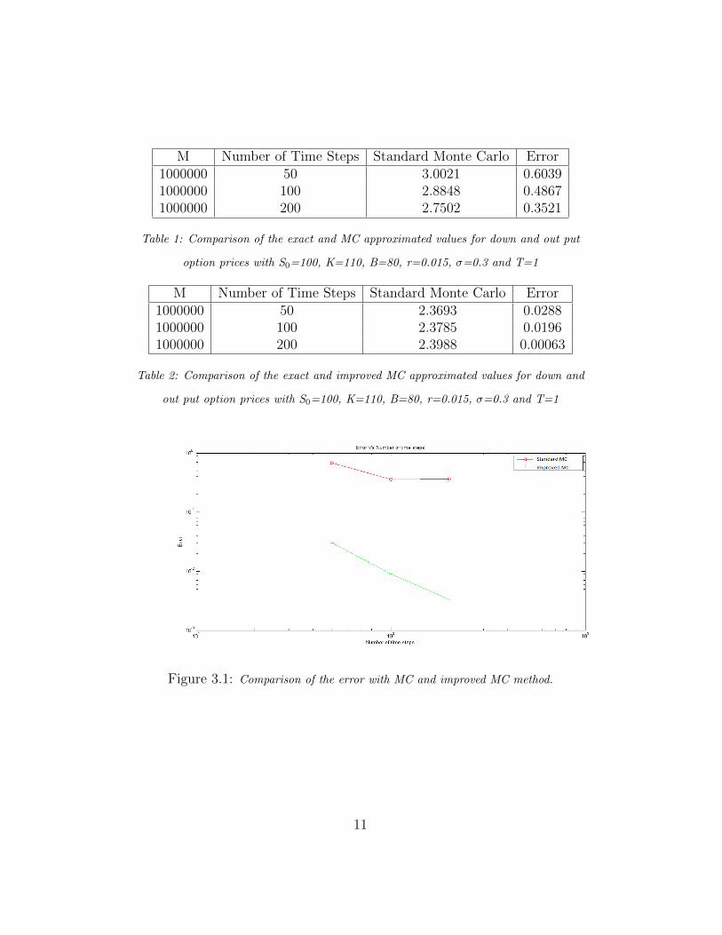
M Number of Time Steps Standard Monte Carlo Error1000000 50 3.0021 0.60391000000 100 2.8848 0.48671000000 200 2.7502 0.3521
Table 1: Comparison of the exact and MC approximated values for down and out put
option prices with S0=100, K=110, B=80, r=0.015, σ=0.3 and T=1
M Number of Time Steps Standard Monte Carlo Error1000000 50 2.3693 0.02881000000 100 2.3785 0.01961000000 200 2.3988 0.00063
Table 2: Comparison of the exact and improved MC approximated values for down and
out put option prices with S0=100, K=110, B=80, r=0.015, σ=0.3 and T=1
Figure 3.1: Comparison of the error with MC and improved MC method.
11
Chapter 4
Stochastic Volatility Model
Black-Scholes model is the most widely used tool in the world of finance. The
main reason behind this is that it has a closed form solution and it requires
almost no computational resources. However, the Black-Scholes model relies
on many assumptions that are unrealistic. One of the main flaws within the
model is the fact that Black-Scholes assumes that market is complete and the
volatility is constant. However, empirical evidence shows that the volatility
behaves in a random manner. To correct these flaws, an extension on the
Black-Scholes model was proposed by Heston in 1993. Heston’s stochastic
volatility can be specified as [8]
dStSt
= rdt+√VtdW
1t (4.1)
dVt = −λ(Vt − V )dt+ η√VtdW
2t (4.2)
E(dW 1t dW
2t ) = ρdt, (4.3)
where r- risk free rate
St - underlying stock price
12
Vt - variance
V - long term mean variance
λ- mean reversion rate
η- volatility of variance
ρ - correlation between the stock price and variance
W1t and W2
t - Wiener stochastic processes
Note that in order to take into account the leverage effect, the Wiener
stochastic processes W1t and W2
t should be correlated E(dW1t dW2
t )=ρ dt.
One of the main drawbacks of this model is that there is no analytical
solution to it. However, we can approximate this solution using Monte Carlo
simulations. In this paper, we will use Milstein method and Quadratical
Exponential Method (QE) method by Leif Andersen to discretize (4.1) and
(4.2).
4.1 Milstein Method
Milstein’s method is a second order numerical scheme used to numerically
solve stochastic differential equations. Consider a general Ito process
dXt = a(Xt)dt+ b(Xt)dWt. (4.4)
From Euler-Maruyama method, the integral below can be approximated as
[15] ∫ tn+1
tn
b(s,Xs)dWs dx ≈ b(tn, Xn)∆Wn. (4.5)
13
Applying Ito formula to (4.4) we get the following [15]
Xti+1= Xti +
∫ ti+1
ti
[a(Xti) +
∫ s
ti
(a′(Xu)a(Xu) +
1
2a′′(Xu)b
2(Xu))du
+
∫ s
ti
a′(Xu)b(Xu)dWu
]ds+
∫ ti+1
ti
[b(Xti) +
∫ s
ti
b′(Xu)(Xu)1
2b′′(Xu)b
2(Xu)du
+
∫ s
ti
1
2b′(Xu)b(Xu)dWu)
]dWs.
If we omit the higher order terms in the formula above, i.e. dWs *du,
dWu*ds, and du*ds, we obtain
Xti+1≈ Xti
∫ ti+1
ti
a(Xti)ds+
∫ ti+1
ti
(b(Xti) +
1
2
∫ s
ti
b′(Xu)b(Xu)dWu
)dWs.
Applying formula (4.5) to the second and third terms gives
≈ Xti + a(Xti)∆t+ b(Xti)∆Wi +1
2
∫ ti+1
ti
∫ s
ti
b′(Xu)b(Xu)dWudWs. (4.6)
The double integral in (4.6) can be approximated as [15]
1
2
∫ ti+1
ti
∫ s
ti
b′(Xu)b(Xu)dWudWs ≈1
2b′(Xti)b(Xti)
((∆Wi)
2 −∆t). (4.7)
By combining equations (4.6) and (4.7), the Milstein’s scheme can be obtain
as follows [15]:
X0 = b(Xt0)
Xti+1= Xti + a(Xi)∆t+ b(Xi)∆Wi +
1
2b′(Xi)b(Xi)
((∆Wi)
2 −∆t). (4.8)
Our main goal is to use scheme (4.8) to discretize the Heston stochastic
volatility. Let Xt=log(St), σ=√V . We apply equation (4.8) to (3.2) and
(4.2) to obtain
Xi+1 = Xi + (r − V
2)∆t+
√V∆tφ(1) +
1
2
√V ∗ 0.
14
where b′(Xi)=0 (since V does not depend on X), a=r-V2
, b=√V and ∆Zt=
√∆tφ
Xi+1 = Xi + (r − V
2)∆t+
√V∆tφ(1) (4.9)
Vi+1 = Vi − λ(V − V )∆t+ η√V√
∆tφ(2) + (1
2η√V )(
1
2
η√V
)(∆t(φ(2))2 −∆t)
Vi+1 = Vi − λ(V − V )∆t+ η√V√
∆tφ(2) +1
4η2∆t(φ(2))2 − 1
4η2∆t
Vi+1 = (√Vi +
η
2
√∆tφ(2))2 − λ(Vi − Vbar)∆t−
1
4η2∆t (4.10)
E(φ(1)φ(2)) = ρdt. (4.11)
Note that equation (4.4) E(dW1t dW2
t )=ρ dt can be discretizes as following
E(φ(1)φ(2)) = ρ (4.12)
where φ(1) and φ(2) are the standard normal distributions with correlation ρ.
Having constructed a numerical scheme for solution of (4.1) and (4.2), we
are almost ready to perform MC simulations. The only missing component
is a generator of standard normal random numbers with correlation ρ.
4.1.1 Generation of Correlated Random Samples φ(1)
φ(2)
Suppose we have a basket of two stocks, S1 and S2. Suppose further that the
returns of these two stocks have correlation -1 ≤ ρ ≤ 1, i.e.
dS1
S1= µ1dt+ σ(1)dW 1
t (4.13)
dS2
S2= µ2dt+ σ(2)dW 2
t (4.14)
E(dW 1t dW
2t ) = ρdt, dZ1 = φ(1)
√dt, dZ2 = φ(2)
√dt, E(φ(1)φ(2)) = ρ.
Before proceeding, we will give a quick overview of a covariance matrix and
its definition. A process for generating covariance matrices is described in
the next section.
15
4.1.2 Covariance Matrices
Let X and Y be two random variables. The covariance of two random vari-
ables is defined as [7]
Cov(X, Y ) = E(X − E(X))E(Y − E(Y )). (4.15)
Let X= (X1, X2, ..., Xp) be a random vector with mean vector µ = (µ1, µ2,
..., µp). Then the covariance matrix Q can be written in the form [7]
Q =
Cov(X1, X1) · · · Cov(X1, Xp)...
. . ....
Cov(Xp, X1) · · · Cov(Xp, Xp)
,where Cov(Xi,Xj) is the covariance of Xi and Xj for i 6= j , and Cov(Xi,Xi)
is the covariance of Xi with itself, that is, its variance Var(Xi). Therefore Q
can be rewritten as:
Q =
V ar(X1) Cov(X1, X2) · · · Cov(X1, Xp)
Cov(X2, X1) V ar(X2)...
.... . .
...Cov(Xp, X1) Cov(Xp, X2) · · · V ar(Xp)
.For example: if X=(X1, X2), Cov(X1,X2)=0.75, Var(X1)=Var(X2)=1, then
the covariance matrix of X is :
Q =
[1 0.75
0.75 1
].
Note, that the covariance matrix is a symmetric positive semi-definite ma-
trix, i.e, for any X ∈ R, XTQX ≥0. Also, for any real covariance matrix the
diagonal entries are greater or equal to zero.
Using these facts, we can now generate correlated normal random variables.
Assume that we have ξ1, ξ2,...., ξn which are independent standard normals
16
i.e. E(ξi)=0, σ(ξi)=1 and E(ξi,ξj)=0 for i 6= j. Let
e =
ξ1
ξ2...ξn
.Let φ=GT e (G is the upper triangular matrix such that Q= GGT which
can be obtained by computing the Cholesky decomposition of Q) satisfying
E(φ)=0.
In Matlab we can compute the Cholesky decomposition of Q using Matlab
command ”chol” [7]. For example, to generate a sample of random vector
with covariance matrix Q, we do the following:
1. Compute G, G= chol(Q).
2. Generate N(0,1) sample Xi (Xi can be computed using randn(n,1) com-
mand).
3. Compute φ1 = GT Xi.
We are now ready to perform Monte Carlo simulations to compute the price
of barrier options. However, since there exists an exact solution for vanilla
call options, we will first compute a vanilla call option and compare the re-
sult with the exact solution. This will serve as a test to check if the model is
working correctly. Its other purpose is to study the accuracy of the model.
Monte Carlo simulations using Milstein discretization for vanilla call option
can be implemented in Matlab using the following pseudocode
17
Compute matrix G and set X=log(S)
For i=1:M
For j=1:N
Generate N(0,1) sample Zj
Compute φ1 and φ2 using matrix G
Compute Xj using (4.9)
Compute Vj using (4.10)
if Vj <0 set Vj =0
End
Sstorei=Sj
End
Set Sstore=eX
Set V=e−rT 1M
M∑i=0
max( Si-K,0);
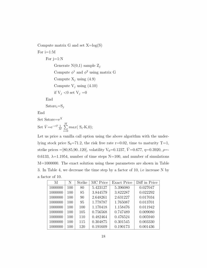
Let us price a vanilla call option using the above algorithm with the under-
lying stock price S0=71.2, the risk free rate r=0.02, time to maturity T=1,
strike prices =[80,85,90..120], volatility V0=0.1237, V=0.677, η=0.3920, ρ=-
0.6133, λ=1.1954, number of time steps N=100, and number of simulations
M=1000000. The exact solution using these parameters are shown in Table
3. In Table 4, we decrease the time step by a factor of 10, i.e increase N by
a factor of 10.
M N Strike MC Price Exact Price Diff in Price1000000 100 80 5.423127 5.396080 0.0270471000000 100 85 3.844579 3.822287 0.0222921000000 100 90 2.648261 2.631227 0.0170341000000 100 95 1.778787 1.765087 0.0137011000000 100 100 1.170418 1.158476 0.0119421000000 100 105 0.756568 0.747489 0.0090801000000 100 110 0.482464 0.476524 0.0059401000000 100 115 0.304875 0.301545 0.0033301000000 100 120 0.191609 0.190173 0.001436
18
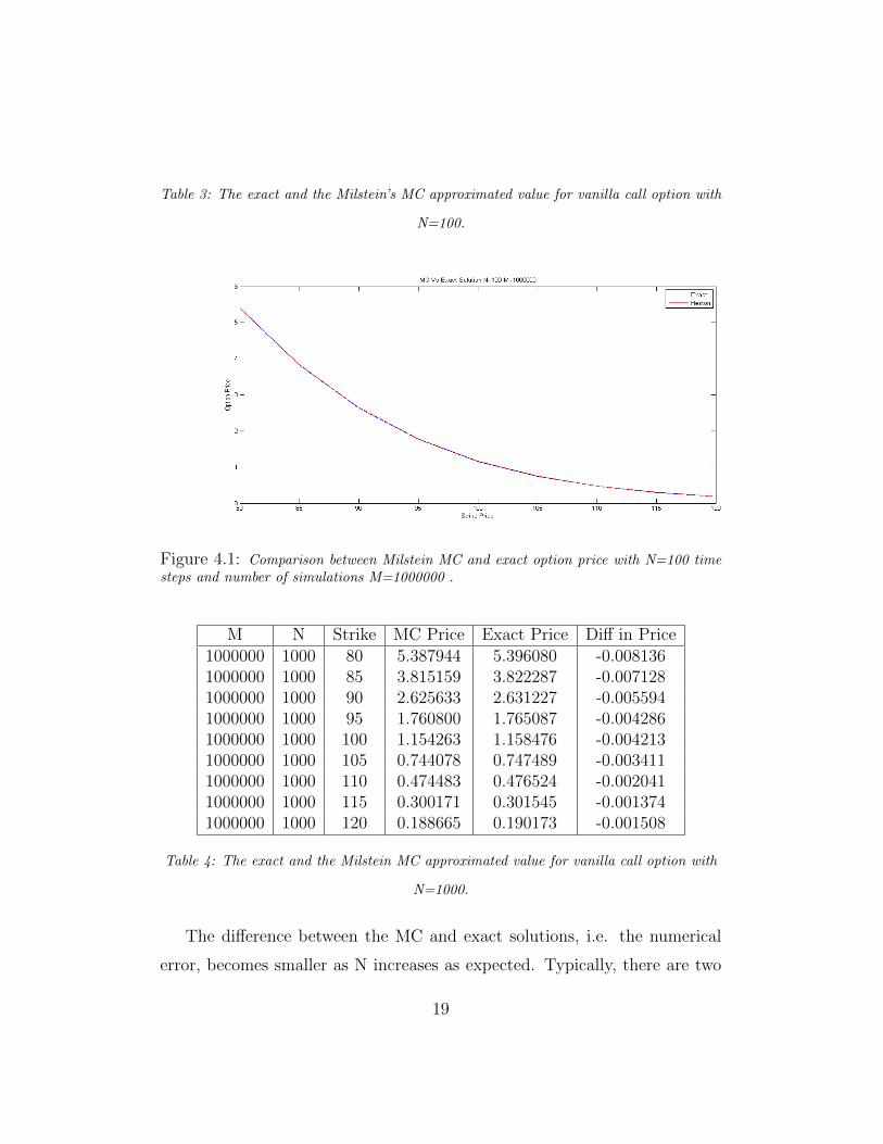
Table 3: The exact and the Milstein’s MC approximated value for vanilla call option with
N=100.
Figure 4.1: Comparison between Milstein MC and exact option price with N=100 timesteps and number of simulations M=1000000 .
M N Strike MC Price Exact Price Diff in Price1000000 1000 80 5.387944 5.396080 -0.0081361000000 1000 85 3.815159 3.822287 -0.0071281000000 1000 90 2.625633 2.631227 -0.0055941000000 1000 95 1.760800 1.765087 -0.0042861000000 1000 100 1.154263 1.158476 -0.0042131000000 1000 105 0.744078 0.747489 -0.0034111000000 1000 110 0.474483 0.476524 -0.0020411000000 1000 115 0.300171 0.301545 -0.0013741000000 1000 120 0.188665 0.190173 -0.001508
Table 4: The exact and the Milstein MC approximated value for vanilla call option with
N=1000.
The difference between the MC and exact solutions, i.e. the numerical
error, becomes smaller as N increases as expected. Typically, there are two
19
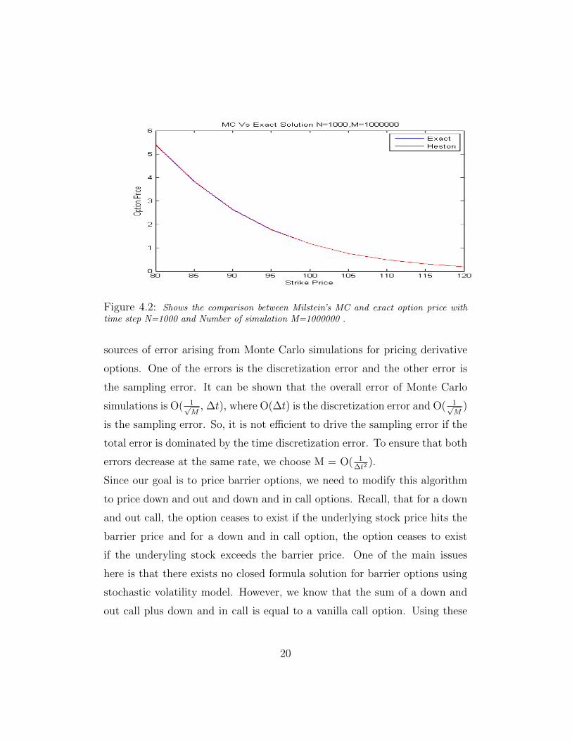
Figure 4.2: Shows the comparison between Milstein’s MC and exact option price withtime step N=1000 and Number of simulation M=1000000 .
sources of error arising from Monte Carlo simulations for pricing derivative
options. One of the errors is the discretization error and the other error is
the sampling error. It can be shown that the overall error of Monte Carlo
simulations is O( 1√M
, ∆t), where O(∆t) is the discretization error and O( 1√M
)
is the sampling error. So, it is not efficient to drive the sampling error if the
total error is dominated by the time discretization error. To ensure that both
errors decrease at the same rate, we choose M = O( 1∆t2
).
Since our goal is to price barrier options, we need to modify this algorithm
to price down and out and down and in call options. Recall, that for a down
and out call, the option ceases to exist if the underlying stock price hits the
barrier price and for a down and in call option, the option ceases to exist
if the underyling stock exceeds the barrier price. One of the main issues
here is that there exists no closed formula solution for barrier options using
stochastic volatility model. However, we know that the sum of a down and
out call plus down and in call is equal to a vanilla call option. Using these
20
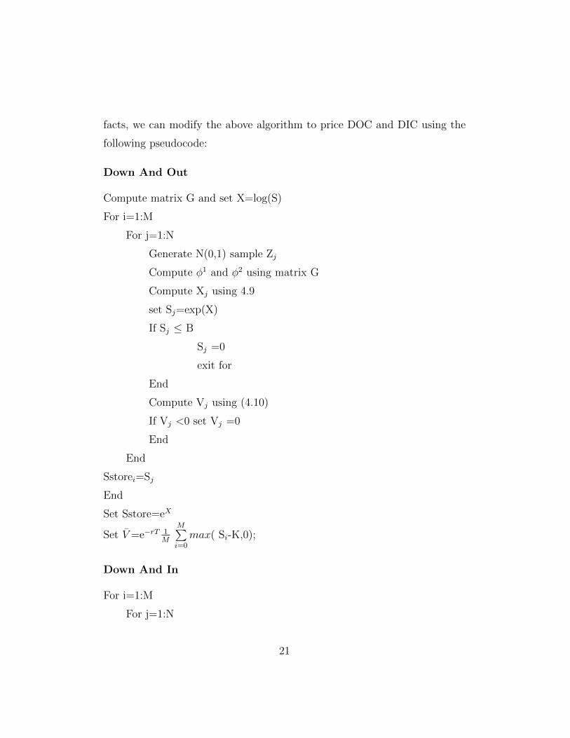
facts, we can modify the above algorithm to price DOC and DIC using the
following pseudocode:
Down And Out
Compute matrix G and set X=log(S)
For i=1:M
For j=1:N
Generate N(0,1) sample Zj
Compute φ1 and φ2 using matrix G
Compute Xj using 4.9
set Sj=exp(X)
If Sj ≤ B
Sj =0
exit for
End
Compute Vj using (4.10)
If Vj <0 set Vj =0
End
End
Sstorei=Sj
End
Set Sstore=eX
Set V=e−rT 1M
M∑i=0
max( Si-K,0);
Down And In
For i=1:M
For j=1:N
21
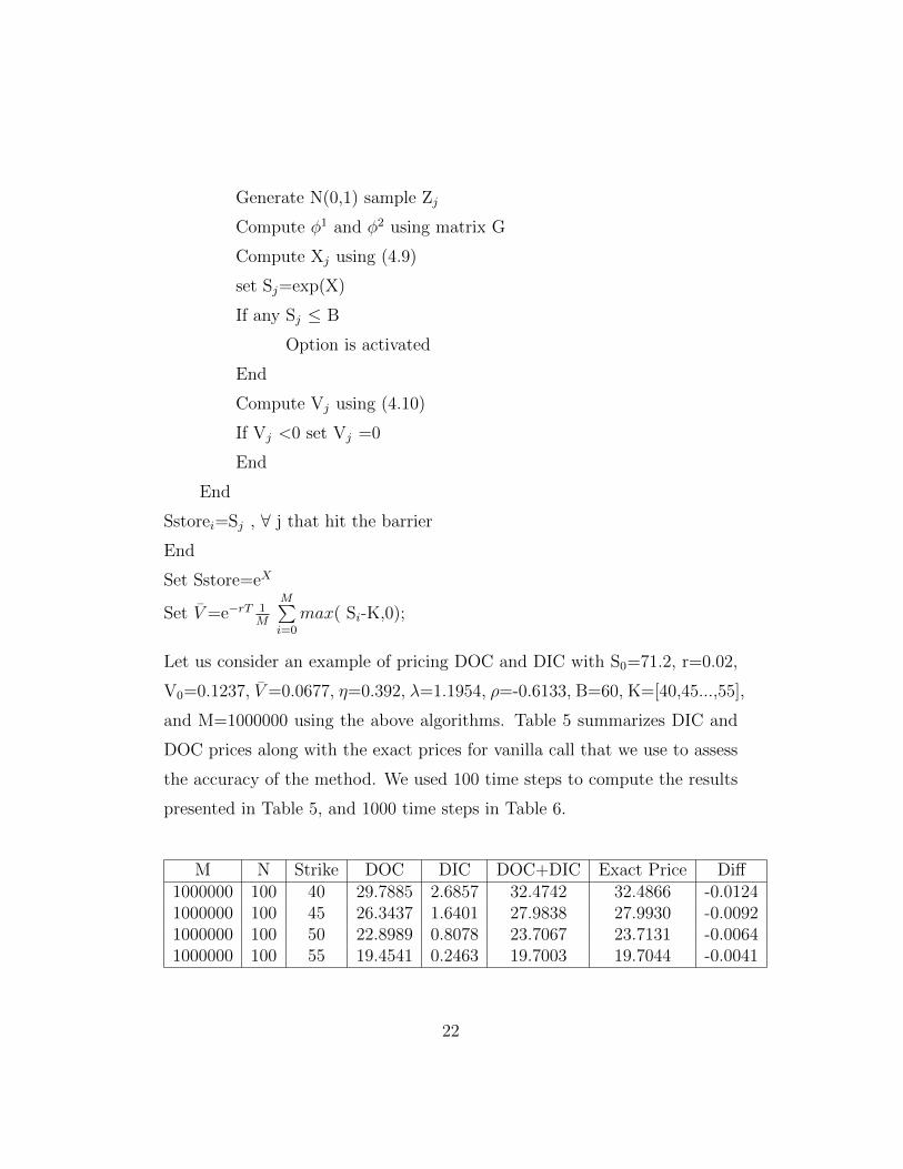
Generate N(0,1) sample Zj
Compute φ1 and φ2 using matrix G
Compute Xj using (4.9)
set Sj=exp(X)
If any Sj ≤ B
Option is activated
End
Compute Vj using (4.10)
If Vj <0 set Vj =0
End
End
Sstorei=Sj , ∀ j that hit the barrier
End
Set Sstore=eX
Set V=e−rT 1M
M∑i=0
max( Si-K,0);
Let us consider an example of pricing DOC and DIC with S0=71.2, r=0.02,
V0=0.1237, V=0.0677, η=0.392, λ=1.1954, ρ=-0.6133, B=60, K=[40,45...,55],
and M=1000000 using the above algorithms. Table 5 summarizes DIC and
DOC prices along with the exact prices for vanilla call that we use to assess
the accuracy of the method. We used 100 time steps to compute the results
presented in Table 5, and 1000 time steps in Table 6.
M N Strike DOC DIC DOC+DIC Exact Price Diff1000000 100 40 29.7885 2.6857 32.4742 32.4866 -0.01241000000 100 45 26.3437 1.6401 27.9838 27.9930 -0.00921000000 100 50 22.8989 0.8078 23.7067 23.7131 -0.00641000000 100 55 19.4541 0.2463 19.7003 19.7044 -0.0041
22
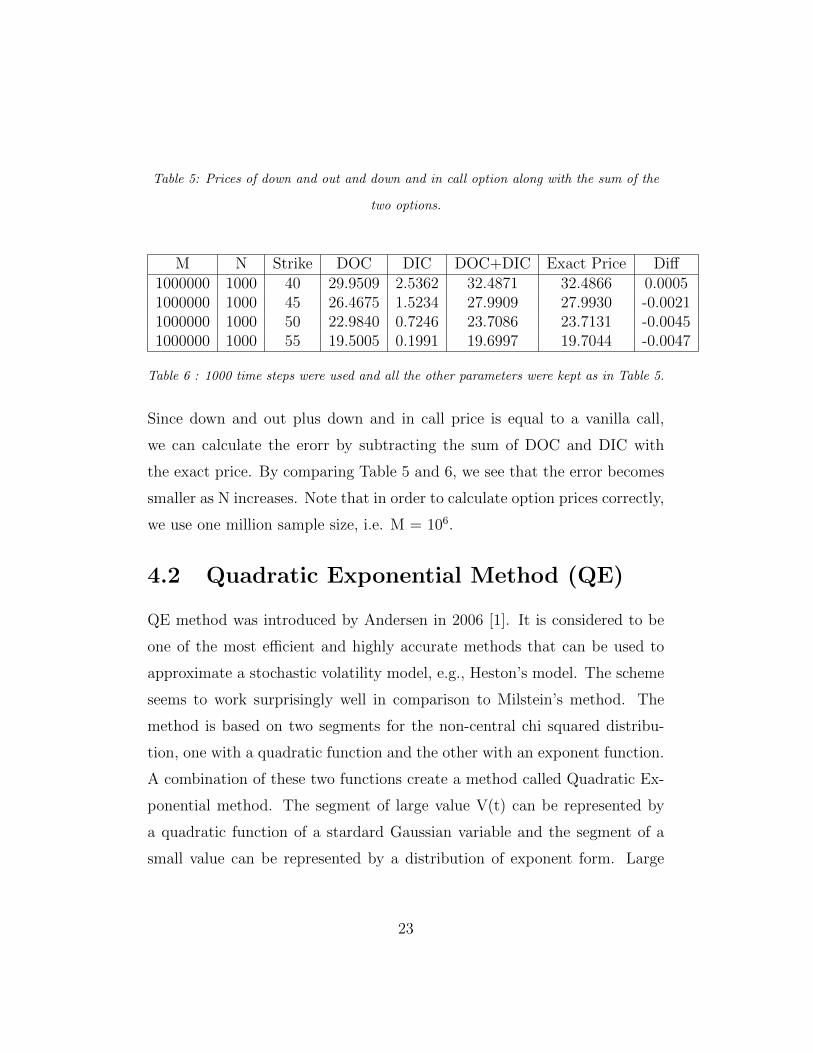
Table 5: Prices of down and out and down and in call option along with the sum of the
two options.
M N Strike DOC DIC DOC+DIC Exact Price Diff1000000 1000 40 29.9509 2.5362 32.4871 32.4866 0.00051000000 1000 45 26.4675 1.5234 27.9909 27.9930 -0.00211000000 1000 50 22.9840 0.7246 23.7086 23.7131 -0.00451000000 1000 55 19.5005 0.1991 19.6997 19.7044 -0.0047
Table 6 : 1000 time steps were used and all the other parameters were kept as in Table 5.
Since down and out plus down and in call price is equal to a vanilla call,
we can calculate the erorr by subtracting the sum of DOC and DIC with
the exact price. By comparing Table 5 and 6, we see that the error becomes
smaller as N increases. Note that in order to calculate option prices correctly,
we use one million sample size, i.e. M = 106.
4.2 Quadratic Exponential Method (QE)
QE method was introduced by Andersen in 2006 [1]. It is considered to be
one of the most efficient and highly accurate methods that can be used to
approximate a stochastic volatility model, e.g., Heston’s model. The scheme
seems to work surprisingly well in comparison to Milstein’s method. The
method is based on two segments for the non-central chi squared distribu-
tion, one with a quadratic function and the other with an exponent function.
A combination of these two functions create a method called Quadratic Ex-
ponential method. The segment of large value V(t) can be represented by
a quadratic function of a stardard Gaussian variable and the segment of a
small value can be represented by a distribution of exponent form. Large
23
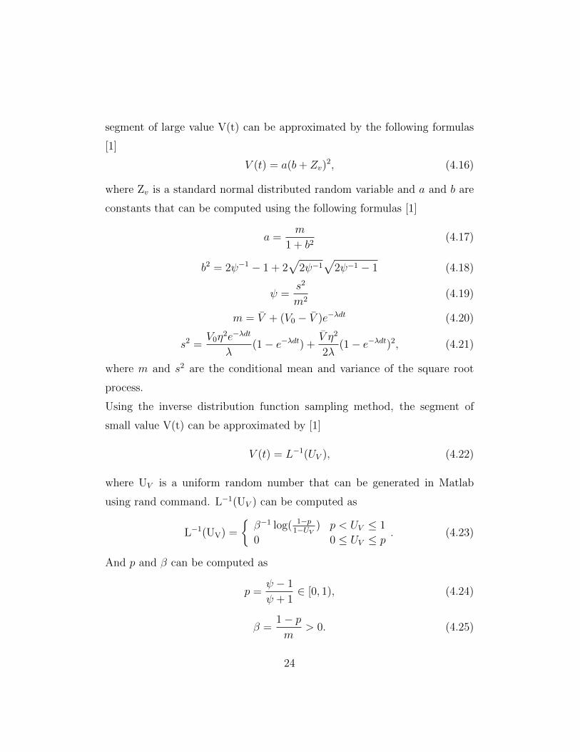
segment of large value V(t) can be approximated by the following formulas
[1]
V (t) = a(b+ Zv)2, (4.16)
where Zv is a standard normal distributed random variable and a and b are
constants that can be computed using the following formulas [1]
a =m
1 + b2(4.17)
b2 = 2ψ−1 − 1 + 2√
2ψ−1√
2ψ−1 − 1 (4.18)
ψ =s2
m2(4.19)
m = V + (V0 − V )e−λdt (4.20)
s2 =V0η
2e−λdt
λ(1− e−λdt) +
V η2
2λ(1− e−λdt)2, (4.21)
where m and s2 are the conditional mean and variance of the square root
process.
Using the inverse distribution function sampling method, the segment of
small value V(t) can be approximated by [1]
V (t) = L−1(UV ), (4.22)
where UV is a uniform random number that can be generated in Matlab
using rand command. L−1(UV ) can be computed as
L−1(UV) =
{β−1 log( 1−p
1−UV) p < UV ≤ 1
0 0 ≤ UV ≤ p. (4.23)
And p and β can be computed as
p =ψ − 1
ψ + 1∈ [0, 1), (4.24)
β =1− pm
> 0. (4.25)
24
4.2.1 Sampling The Underlying Stock Price
Suppose that the asset price can be modelled using equation (4.1) and the
variance process can be modelled using equation (4.2). Applying Ito’s for-
mula to (4.1), the underlying stock price can be written as [1]
S(t) = S(s)e∫ ts (r− 1
2V (u))du+
∫ ts
√V (u)dW (1)
. (4.26)
Using the Cholesky decomposition we obtain the following equation
log(S(t)) = log(S(s)) +
∫ t
s
rdu− 1
2
∫ t
s
v(u)du+ ρ
∫ t
s
√v(u)dW (2)
+√
1− ρ2
∫ t
s
√v(u)dW (1). (4.27)
Integrating the variance process (4.2) we obtain
V (t) = V (s) +
∫ t
s
−λ(V (u)− V )du+ η
∫ t
s
√V (u)dW (2)du, (4.28)
or, equivalently,∫ t
s
√V (u)dW (2)du =
V (t)− V (s)− λV∆t+ λ∫ tsV (u)du
η. (4.29)
Substituting (4.27) into (4.26), results in the Broadie-Kaya scheme [4]
log(S(t) = log(S(s)) + r∆t+λρ
η
∫ t
s
V (u)du− 1
2
∫ t
s
V (u)du
+ρ
η(V (t)− V (s)− λV∆t) +
√1− ρ2
∫ t
s
√V (u)dW (1).
(4.30)
The only issue left to be addressed in (4.28) is the the integrand of the
variance process. Applying the drift interpolation method to approximate
the integral of the variance process, we obtain [6]∫ t
s
V (u)du ≈ (α1V (s) + α2V (t))∆t, (4.31)
25
where α1 and α2 are constants. There are many ways of assigning these
constants, the simplest one is the Euler-like setting:α1=1 and α2=0. The
other way is the mid-point discretization method that would set α1=α2=12.
Substituting equation (4.31) into (4.30) using the mid-point discretization
we obtain
log(S(t)) = log(S(s)) + r∆t+λρ
η(α1V (s) + α2V (t))∆t
−1
2(α1V (s) + α2V (t))∆t+
ρ
η(V (t)− V (s)− λV∆t)
+√
1− ρ2√α1V (s) + α2V (t)
√∆tφ.
(4.32)
or, equivalently, [1]
log(S(t)) = log(S(s)) + r∆t+K0 +K1V (s) +K2V (t)
+√K3V (s) +K4V (t)
√∆tφ, (4.33)
where φ is a Wiener stochastic process and K0, K1, K2, K3, K4 are given by:
K0 = −ρλVη
∆t, K1 = α1∆t(λρ
η− 1
2)− ρ
η, K2 = α2∆t(
λρ
η− 1
2) +
ρ
η
K3 = α1∆t√
1− ρ2, K4 = α2∆t√
1− ρ2
Quadratic Exponential (QE) Algorithm
[1] Assuming that some critical arbitrary switch level φc ∈[1,2] is given
and supposing the mid-point discretization α1=α2=12
has been chosen, the
Quadratic Exponential algorithm can be summarized as follows:
1. Given V(s), V , η, λ, compute m, s2, and ψ.
2. Generate UV using rand command.
3. If ψ ≤ ψc
26
(a) Compute a and b.
(b) Compute ZV .
(c) Compute segment of large value V(t) using (4.16).
4. if ψ > ψc
(a) Compute p and β.
(b) Compute segment of small value V(t) using (4.22) and (4.23).
5. Compute K0,..,K4.
6. Compute log(S(t)) using (4.33).
7. Take the exponential of log(S(t)) and compute the payoff of the option.
For more details, see Leif Andersen’s paper December 12, 2006 version [1].
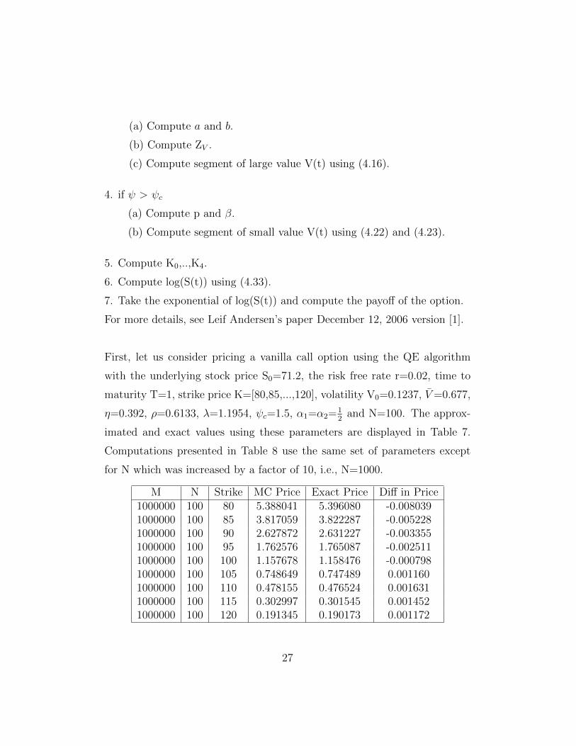
First, let us consider pricing a vanilla call option using the QE algorithm
with the underlying stock price S0=71.2, the risk free rate r=0.02, time to
maturity T=1, strike price K=[80,85,...,120], volatility V0=0.1237, V=0.677,
η=0.392, ρ=0.6133, λ=1.1954, ψc=1.5, α1=α2=12
and N=100. The approx-
imated and exact values using these parameters are displayed in Table 7.
Computations presented in Table 8 use the same set of parameters except
for N which was increased by a factor of 10, i.e., N=1000.
M N Strike MC Price Exact Price Diff in Price1000000 100 80 5.388041 5.396080 -0.0080391000000 100 85 3.817059 3.822287 -0.0052281000000 100 90 2.627872 2.631227 -0.0033551000000 100 95 1.762576 1.765087 -0.0025111000000 100 100 1.157678 1.158476 -0.0007981000000 100 105 0.748649 0.747489 0.0011601000000 100 110 0.478155 0.476524 0.0016311000000 100 115 0.302997 0.301545 0.0014521000000 100 120 0.191345 0.190173 0.001172
27
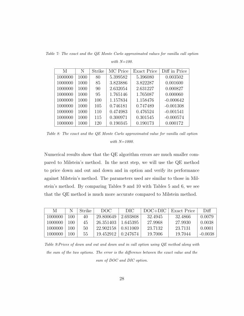
Table 7: The exact and the QE Monte Carlo approximated values for vanilla call option
with N=100.
M N Strike MC Price Exact Price Diff in Price1000000 1000 80 5.399582 5.396080 0.0035021000000 1000 85 3.823886 3.822287 0.0016001000000 1000 90 2.632054 2.631227 0.0008271000000 1000 95 1.765146 1.765087 0.0000601000000 1000 100 1.157834 1.158476 -0.0006421000000 1000 105 0.746181 0.747489 -0.0013081000000 1000 110 0.474983 0.476524 -0.0015411000000 1000 115 0.300971 0.301545 -0.0005741000000 1000 120 0.190345 0.190173 0.000172
Table 8: The exact and the QE Monte Carlo approximated value for vanilla call option
with N=1000.
Numerical results show that the QE algorithm errors are much smaller com-
pared to Milstein’s method. In the next step, we will use the QE method
to price down and out and down and in option and verify its performance
against Milstein’s method. The parameters used are similar to those in Mil-
stein’s method. By comparing Tables 9 and 10 with Tables 5 and 6, we see
that the QE method is much more accurate compared to Milstein method.
M N Strike DOC DIC DOC+DIC Exact Price Diff1000000 100 40 29.800649 2.693808 32.4945 32.4866 0.00791000000 100 45 26.351403 1.645395 27.9968 27.9930 0.00381000000 100 50 22.902158 0.811069 23.7132 23.7131 0.00011000000 100 55 19.452912 0.247674 19.7006 19.7044 -0.0038
Table 9:Prices of down and out and down and in call option using QE method along with
the sum of the two options. The error is the difference between the exact value and the
sum of DOC and DIC option.
28
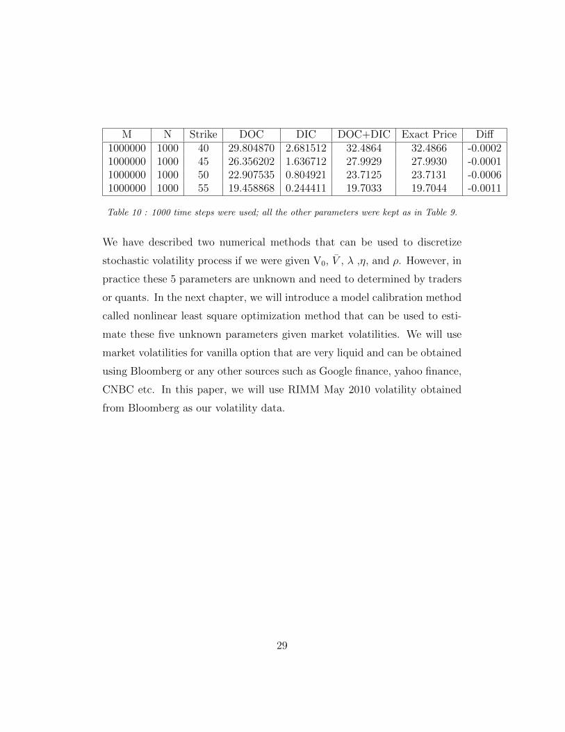
M N Strike DOC DIC DOC+DIC Exact Price Diff1000000 1000 40 29.804870 2.681512 32.4864 32.4866 -0.00021000000 1000 45 26.356202 1.636712 27.9929 27.9930 -0.00011000000 1000 50 22.907535 0.804921 23.7125 23.7131 -0.00061000000 1000 55 19.458868 0.244411 19.7033 19.7044 -0.0011
Table 10 : 1000 time steps were used; all the other parameters were kept as in Table 9.
We have described two numerical methods that can be used to discretize
stochastic volatility process if we were given V0, V , λ ,η, and ρ. However, in
practice these 5 parameters are unknown and need to determined by traders
or quants. In the next chapter, we will introduce a model calibration method
called nonlinear least square optimization method that can be used to esti-
mate these five unknown parameters given market volatilities. We will use
market volatilities for vanilla option that are very liquid and can be obtained
using Bloomberg or any other sources such as Google finance, yahoo finance,
CNBC etc. In this paper, we will use RIMM May 2010 volatility obtained
from Bloomberg as our volatility data.
29
Chapter 5
Model Calibration
Model Calibration is an optimization technique used to estimate local volatil-
ity or Heston’s parameters for dependent exotic options that are not very
liquid; thus, their volatilities are not obtainable from the market. It ensures
that the resulting model is consistent with the current market option price
information or, in other words, by using model calibration, the model will
price consistently with market implied volatility. In this chapter, we will use
model calibration to estimate Heston’s parameters by solving a nonlinear
least square optimization problem. We will first introduce a nonlinear least
square problem, and then attempt to solve it using the Levenberg-Marquardt
method. We start with a set of market volatilities and perform an iterative
process to solve nonlinear least square problem using a Matlab command
called lsqnonlin.
Let us suppose that a set of liquid options implied volatilities Volmarket on
an underlying asset are observed from the option market. Suppose that we
can price these options using Black-Scholes model and denote the price by
Vmarket0 (Kj,T) for j=1,2,...m. Assume V0(Kj,T,X), X∈{ v0,V ,λ,η,ρ } denotes
the initial value that can be obtained using Milstein’s method. A model can
30
be calibrated by solving the following equations [2]
V0(Kj, T,X)− V market0 (Kj, T ) = 0, j = 1, 2, ...,m (5.1)
or
minX
m∑j=1
(V0(Kj, T,X)− V market0 (Kj, T ))2, (5.2)
or, equivalently,
minX
1
2‖F (X)‖2
2, (5.3)
where X consists of Heston’s parameters described above, and F(X) can be
written as
F (X) =
V0(K1, T,X)− V market0 (K1, T )
...V0(Km, T,X)− V market
0 (Km, T )
. (5.4)
Solving a nonlinear least square problem is often not straightforward. How-
ever, there are many available iterative methods that can be used to solve
this problem. In this paper, we will use the Levenberg-Marquardt method
to solve equation (5.3).
5.1 Levenberg-Marquardt (LM) method
LM is an iterative method that seeks the minimum of a function expressed as
the sum of squares of nonlinear functions. It is a combination of the steepest
descent and Gauss-Newton methods. The method uses the steepest descent
when the current solution is far from the exact solution, and switches to the
Gauss-Newton method when the current solution is close to the actual solu-
tion. It determines Xnew via solving a trust region subproblem for some ∆old
≥ 0 i.e. [13]
minxnew
1
2‖F (Xnew) + J(Xold)(Xnew −Xold)‖2
2 (5.5)
31
subject to
‖X −Xold‖2 ≤ ∆old, (5.6)
where J(X) is the m by n Jacobian matrix of F(X) that can be written as
[13]
J(X) =
∂F1
∂X1
∂F1
∂X2· · · ∂F1
∂Xn∂F2
∂X1
∂F2
∂X2· · · ∂F2
∂Xn...
.... . .
...∂Fm
∂X1
∂Fm
∂X2· · · ∂Fm
∂Xn
(5.7)
It can be showed that the solution to the trust region (5.5), (5.6) subproblem
has the form
Xnew = Xold +(J(Xold)
TJ(Xold) + λoldI)−1
dold, (5.8)
where
dold = −aJ(Xold)TF (Xold) (5.9)
where a is chosen to minimize (5.5) and λ is the largest value in the interval
[0,1] that controls both the magnitude and direction of dold such that ‖dold‖≤ ∆old. The sketch of the proof is outlined below.
The goal is to find a vector X such that all Fi(X) = 0. By Levenberg-
Marquardt [12], [5] we have(J(Xold)
TJ(Xold) + λoldI)dold = −J(Xold)
TF (Xold)(J(Xold)
TJ(Xold) + λoldI)(− aJ(XT
old)F (Xold))
= −J(Xold)TF (Xold)
−J(XTold)F (Xold) = −a
(J(Xold)
TJ(Xold) + λoldI)−1(
J(Xold)TF (Xold)
)0 = J(XT
old)F (Xold)− a(J(Xold)
TJ(Xold) + λoldI)−1(
J(Xold)TF (Xold)
)
32
Applying the Gauss-Newton method we obtain
Xnew = Xold +(J(Xold)
TJ(Xold) + λoldI)−1
dold.
Note that when λold is zero, the direction dold is given by the Gauss-Newton
method. When λ approaches infinity, the direction dold is the steepest descent
direction, with the magnitude tending to zero. The full proof is beyond
the scope of this paper. Interested reader can be referred to Mathworks
website under Trust-Region Dogleg and Levenberg-Marquardt method for
more details.
The advantage of this method is that it only uses the Jacobian matrix in
the equation. The Jacobian matrix can be easily approximated using finite
difference method. In this paper, we will use the forward difference in time
to approximate the Jacobian matrix, i.e.
J(X) =∂Fj∂Xi
≈ Fj(Xoldi + ∆X)− Fj(Xoldi)
∆X, (5.10)
where i represents the index for the independent variable, j represents the
index of F and ∆X is the spacing.
5.1.1 Matlab Function lsqnonlin
Matlab has a build-in function lsqnonlin that can be used to solve nonlinear
least squares problem. lsqunonlin takes in the function of the a nonlinear
least square F(X), the initial guess X0, and the options as inputs. Below is
the function’s formal way of writing it.
Xnew = lsqnonlin(F (X), X0, options), (5.11)
where options can be set as follows
options=optimset(’Jacobian’,’on’,’Display’,’iter’,’MaxIter’,n).
33
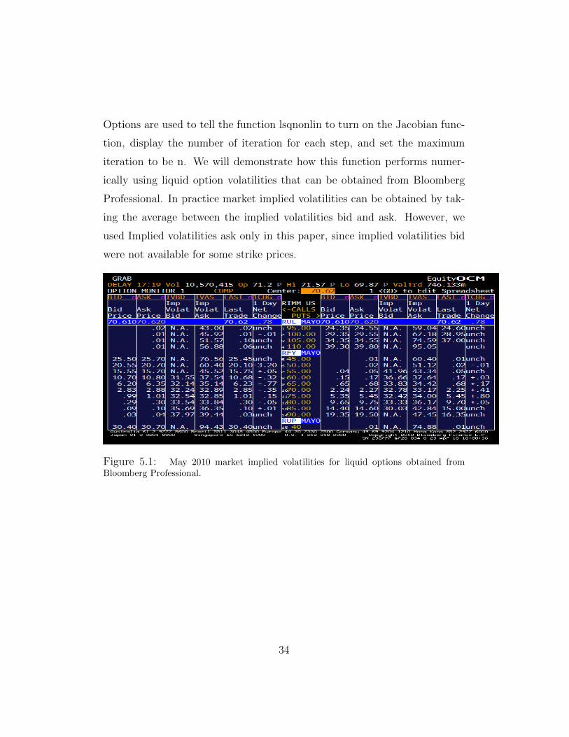
Options are used to tell the function lsqnonlin to turn on the Jacobian func-
tion, display the number of iteration for each step, and set the maximum
iteration to be n. We will demonstrate how this function performs numer-
ically using liquid option volatilities that can be obtained from Bloomberg
Professional. In practice market implied volatilities can be obtained by tak-
ing the average between the implied volatilities bid and ask. However, we
used Implied volatilities ask only in this paper, since implied volatilities bid
were not available for some strike prices.
Figure 5.1: May 2010 market implied volatilities for liquid options obtained fromBloomberg Professional.
34
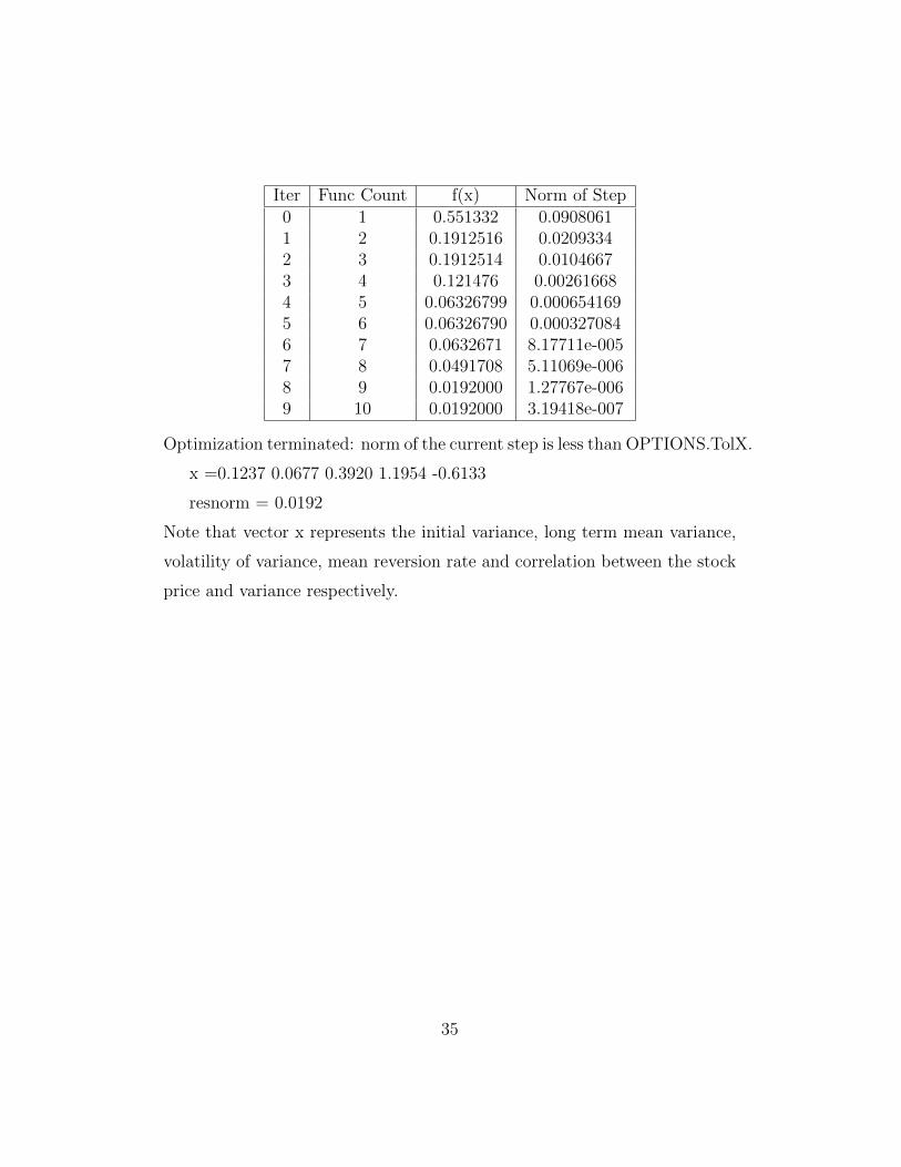
Iter Func Count f(x) Norm of Step0 1 0.551332 0.09080611 2 0.1912516 0.02093342 3 0.1912514 0.01046673 4 0.121476 0.002616684 5 0.06326799 0.0006541695 6 0.06326790 0.0003270846 7 0.0632671 8.17711e-0057 8 0.0491708 5.11069e-0068 9 0.0192000 1.27767e-0069 10 0.0192000 3.19418e-007
Optimization terminated: norm of the current step is less than OPTIONS.TolX.
x =0.1237 0.0677 0.3920 1.1954 -0.6133
resnorm = 0.0192
Note that vector x represents the initial variance, long term mean variance,
volatility of variance, mean reversion rate and correlation between the stock
price and variance respectively.
35
Chapter 6
Numerical Solution of OptionPricing Using Finite DifferenceMethod
As described earlier in Chapter 4, Heston model has no closed form formulas
for any exotic options except for the simplest, and therefore numerical meth-
ods need to be used. In this chapter, we will use finite difference method
to discretize Heston partial differential equation (PDE) that plays an impor-
tant role in the financial market. We will first introduce Heston PDE and
its parameters. Then we describe the explicit and implicit schemes we used
to solve this PDE. Various numerical examples will be shown using the same
parameters as those in Chapter 5. We will consider vanilla call option as well
as down and out and down and in barrier options.
6.1 Heston PDE
Applying Ito’s lemma and the standard arbitrage arguments to equation (4.1)
and (4.2) we arrive at Heston’s partial differential equation [9]
∂U
∂t=
1
2s2v
∂U2
∂s2+ρηsv
∂U2
∂s∂v+
1
2η2v
∂U2
∂v2+(r−q)s∂U
∂s+λ(v−v)
∂U
∂v−ru. (6.1)
36
This PDE is a two dimensional time dependent convection-diffusion-reaction
equation, where r is the risk-free rate, q is the dividend rate and U(s,v,t)
is the option price for 0 ≤ t ≤ T , s> 0 , v> 0. The initial condition for
European call option can be given as [9]
U(s, v, 0) = max(0, s−K). (6.2)
The boundary condition at s=0 can be written as follows
U(0, v, t) = 0. (6.3)
For down and out call option, the initial condition can be given by
U(B, v, t) = 0. (6.4)
Note that the two dimensional domain for this PDE is unbounded from
above. In this paper, we will restrict the domain to a bounded set [0,S] x
[0,V] where S and V are sufficiently large. The boundary conditions at s=S
and v=V are set to [9]∂U
∂s(S, v, t) = e−qt, (6.5)
U(s, V, t) = se−qt. (6.6)
For down and out call option equation (6.6) changes to
U(s, V, t) = (s−B)e−qt. (6.7)
and equation (6.5) stays the same.
6.1.1 Setting Up Non Uniform Grid
Non uniform meshes in both s and v direction will be used in this finite differ-
ence scheme, since we are interested in the solution that lies near (s,v)=(K,0)
37
only. A mesh is constructed in a way such that more points are located near
points of interest and the mesh is constructed sparse elsewhere. Building the
grid this way allows us to greatly improve the accuracy of the finite difference
discretization scheme compared to the use of a uniform grid. The non uni-
form grid that we will be using in this section has recently been considered
by Tavella, Randall and Kluge [9]. Let the equidistant points be ξi i.e [9]
ξi = sinh−1(−K/c) + i∆ξ (0 ≤ i ≤ m1), (6.8)
where m1 is an integer greater or equal to 1 and c > 0 is a constant. The
spacing ∆ ξ can be written as,
∆ξ =1
m1
(sinh−1
((S −K)/c
)− sinh−1(−K/c)
). (6.9)
Then the s grid can be defined as
si = K + csinh(ξi), (0 ≤ i ≤ m1). (6.10)
For down and out call option equations (6.8) and (6.9) change to
ξi = sinh−1((B −K)/c) + i∆ξ (0 ≤ i ≤ m1), (6.11)
∆ξ =1
m1
(sinh−1
((S −K)/c
)− sinh−1((B −K)/c)
). (6.12)
Now for v grid, let the equidistant points be ηi [9]
ηj = j∆η, (6.13)
with spacing
∆η =1
m2
sinh−1(V/d), (6.14)
where m2 is an integer greater or equal to 1 and d > 0 is a constant. Then
v grid can be defined as
vj = dsinh(ηj), (0 ≤ j ≤ m2). (6.15)
38
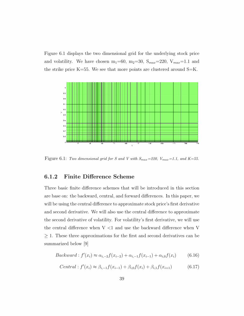
Figure 6.1 displays the two dimensional grid for the underlying stock price
and volatility. We have chosen m1=60, m2=30, Smax=220, Vmax=1.1 and
the strike price K=55. We see that more points are clustered around S=K.
Figure 6.1: Two dimensional grid for S and V with Smax=220, Vmax=1.1, and K=55.
6.1.2 Finite Difference Scheme
Three basic finite difference schemes that will be introduced in this section
are base on: the backward, central, and forward differences. In this paper, we
will be using the central difference to approximate stock price’s first derivative
and second derivative. We will also use the central difference to approximate
the second derivative of volatility. For volatility’s first derivative, we will use
the central difference when V <1 and use the backward difference when V
≥ 1. These three approximations for the first and second derivatives can be
summarized below [9]
Backward : f ′(xi) ≈ αi,−2f(xi−2) + αi,−1f(xi−1) + αi,0f(xi) (6.16)
Central : f ′(xi) ≈ βi,−1f(xi−1) + βi,0f(xi) + βi,1f(xi+1) (6.17)
39
Forward : f ′(xi) ≈ γi,0f(xi) + γi,1f(xi+1) + γi,2f(xi+2) (6.18)
with the coefficients given by
αi,−2 =∆xi
∆xi−1(∆xi−1 + ∆xi), αi,−1 =
−∆xi−1 −∆xi∆xi−1∆xi
, αi,0 =∆xi−1 + 2∆xi
∆xi(∆xi−1 + ∆xi)
βi,−1 =−∆xi+1
∆xi(∆xi + ∆xi+1), βi,0 =
∆xi+1 −∆xi∆xi∆xi+1
, βi,1 =∆xi
∆xi+1(∆xi + ∆xi+1)
γi,0 =−2∆xi+1 −∆xi+ 2
∆xi+1(∆xi+1 + ∆xi+2), γi,1 =
∆xi+1 + ∆xi+2
∆xi+1∆xi+2
, γi,2 =−∆xi+1
∆xi+2(∆xi+1 + ∆xi+2)
The second derivative can be approximated by [9]
f ′′(xi) ≈ δi,−1f(xi−1) + δi,0f(xi) + δi,1f(xi+1) (6.19)
with the coefficients given by
δi,−1 =2
∆xi(∆xi + ∆xi+1), δi,0 =
−2
∆xi∆xi+1
, δi,1 =2
∆xi+1(∆xi + ∆xi+1).
Let βi,k be the coefficient analogous to βi,k but in the y direction instead of
x, then the mixed derivative of S and V can be approximated by [9]
∂2f
∂x∂y(xi, yj) ≈
1∑k,l=−1
βi,kβj,lf(xi+k, yj+l). (6.20)
6.1.3 ADI Scheme
The finite difference discretization of the Heston partial differential equation
yields an initial value problem for a large ODE system of the form
Fj(t, U) = AjU + bj(t)− rU, for 0 ≤ t ≤ T, U ∈ <m, (6.21)
where j=0,1,2, F=F0+F1+F2, and A=A0+A1+A2.
A0 corresponds to the mixed derivative term ∂U∂s∂v
.
A1 corresponds to the underlying stock price’s first and second derivative
40
terms ∂U∂s
, ∂2U∂s2
.
A2 corresponds to the variance of the first and second derivative terms ∂U∂v
,
∂2U∂v2
.
Let θ be a given real parameter, then the three ADI schemes for the initial
value problem (6.21) can be written as
Forward Euler Method:
U = Un−1 + ∆tF (tn−1, Un−1). (6.22)
Douglas (Do) scheme (Implicit):[11]U0 = Un−1 + ∆tF (tn−1, Un−1),Uj = Uj−1 + θ∆t
(Fj(tn, Uj)− Fj(tn−1, Un−1)
), (j = 1, 2),
Un = U2.(6.23)
Craig Sneyd (CS) Method:[10]U0 = Un−1 + ∆tF (tn−1, Un−1),Uj = Uj−1 + θ∆t
(Fj(tn, Uj)− Fj(tn−1, Un−1)
), (j = 1, 2),
U0 = U0 + 12∆t(F0(tn, U2)− F0(tn−1, Un−1)),
Uj = ˆUj−1 + θ∆t(Fj(tnUj)− Fj(tn−1, Un−1)), (j = 1, 2),
Un = U2.
(6.24)
We will apply forward Euler and Craig-Sneyd methods to price DOC and
DIC barrier options. We will first rewrite these equations so that they can
be coded up in Matlab. For forward Euler method, we do the following
U = Un−1 + ∆t(AUn−1 +B − rUn−1). (6.25)
41
Derivation for Craig-Sneyd can be done as follows
U0 = Uold + ∆t(AUold +B − rUold)
U1 = U0 + θ∆t(A1U1 + b1 − rU1 − A1Uold − b1 + rUold)
U1 − θ∆t(A1U1 − rU1) = U0 + θ∆t(b1 − A1Uold − b1 + rUold)
(I − θ∆t(A1 − rI))U1 = U0 + θ∆t(−A1Uold + rUold)
U1 = (I − θ∆t(A1 − rI))−1(U0 + θ∆t(rUold − A1Uold))
U2 = (I − θ∆t(A2 − rI))−1(U1 + θ∆t(rUold − A2Uold))
U0 = U0 +1
2∆t(A0U2 + b0 − rU2 − (A0Uold + b0 − rUold))
U0 = U0 +1
2∆t(A0U2 − rU2 − A0Uold + rUold)
U1 = U0 + θ∆t(A1U1 + b1 − rU1 − A1Uold − b1 + rUold
U1 = (I − θ∆t(A1 − rI))−1(U0 + θ∆t(rUold − A1Uold))
U2 = (I − θ∆t(A2 − rI))−1(U1 + θ∆t(rUold − A2Uold))
U = U2.
Tables below contain a list of DOC and DIC barrier option prices using
the forward Euler and Crag-Sneyd methods respectively. Heston parameters
were kept as in Chapter 5, with strike price of K=55, stock price S0=71.2,
risk free interest rate r=0.02, Smax=220, Vmax=1.1, and time to maturity
T=1.
Grid Size DIC DOC DIC+DOC Exact Solution Diff15x30 0.1813034 19.7239852 19.9052886 19.7043924 0.200896130x60 0.1472834 19.6218048 19.7690881 19.7043924 0.064695760x120 0.1685462 19.5756501 19.7441963 19.7043924 0.0398038
Table 11: The exact and the forward Euler method value for DOC and DIC barrier
options.
42
Grid Size DIC DOC DIC+DOC Exact Solution Diff15x30 0.1813032 19.7241404 19.9054436 19.7043924 0.201051230x60 0.1472857 19.6217907 19.7690764 19.7043924 0.064684060x120 0.1685463 19.5756467 19.7441930 19.7043924 0.0398006
Table 12: The exact and the Crag-Sneyd method value for DOC and DIC barrier options.
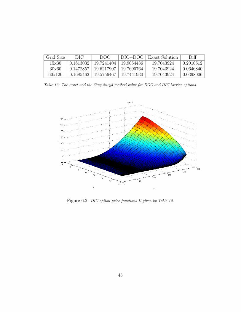
Figure 6.2: DIC option price functions U given by Table 12.
43
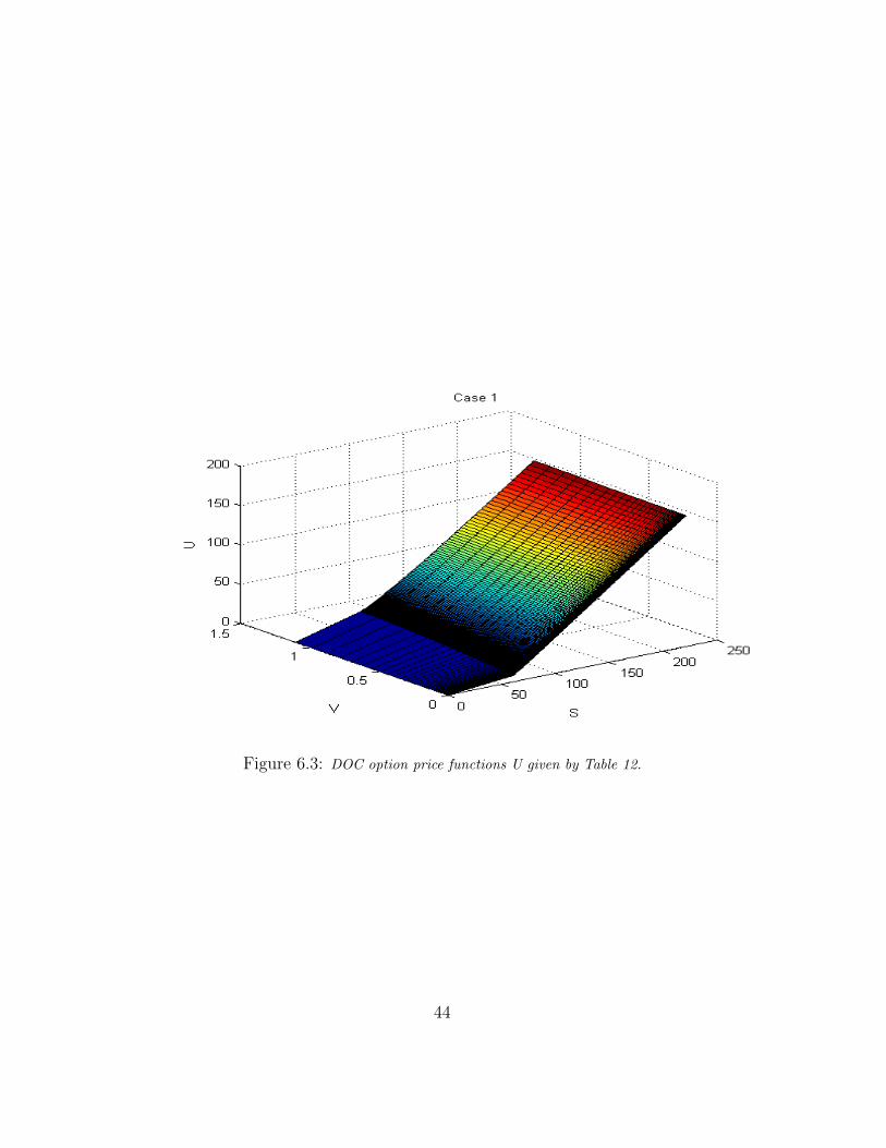
Figure 6.3: DOC option price functions U given by Table 12.
44
Conclusion
In this paper, we have considered several numerical methods to price down
and out, and down and in barrier options. Firstly, we compared the accuracy
of the standard Monte Carlo and improved Monte Carlo methods applied
to the Black-Scholes model. From our numerical experiment, we can see
that improved MC method is much more accurate than the standard MC.
Secondly, we considered two discretization schemes, Milstein and QE, to be
used in Monte Carlo simulations of Heston models. From our numerical
experiments, we can clearly see that the QE is somewhat slower than the
Milstein method. However, in term of accuracy, the QE scheme performs
much better than Milstein’s.
Finally, we considered the finite difference methods. We used two time in-
tegration schemes: forward Euler and CS. For a given time step, Craig-Sneyd
is unconditionally stable with the order of convergence equal to two. The
forward Euler method seems to be slightly faster in time, but the obtained
solutions are less accurate compare to CS scheme. Interested reader can use
numerical methods described in this paper to price more exotic options such
as double barrier options and digital options. We conclude, that the best
results were obtained by using improved MC of [14] and the QE method [1].
Finite difference discretization provides accurate solutions, but at the price
of large CPU and memory requirements.
45

Appendix
Exact solution for down and out put option using Black-Scholes Matlab
code. All the formulas were obtained from [18].
function [V] = Exact(k,Sd,r,sigma,T)
% this program is written to price down and out barrier put option.
%Input *****************************************
% "k" - Strike Price
% "Sd" - Barrier Price
% "r" - Risk Free Interest Rate
% "sigma" - Volatility
% "T" - Time to maturity
%*****************************************
% Initial stock prices
%So=[80:2:120];
So=100;
% d1-d8 are formulas describe in the paper
% use to price option value
d1=(log(So./k)+(r+1/2*sigma^2)*(T))/(sigma*sqrt(T));
d2=(log(So./k)+(r-1/2*sigma^2)*T)/(sigma*sqrt(T));
d3=(log(So./Sd)+(r+1/2*sigma^2)*T)/(sigma*sqrt(T));
d4=(log(So./Sd)+(r-1/2*sigma^2)*T)/(sigma*sqrt(T));
d5=(log(So./Sd)-(r-1/2*sigma^2)*T)/(sigma*sqrt(T));
d6=(log(So./Sd)-(r+1/2*sigma^2)*T)/(sigma*sqrt(T));
d7=(log((So*k)./Sd^2)-(r-1/2*sigma^2)*T)/(sigma*sqrt(T));
46

d8=(log((So*k)./Sd^2)-(r+1/2*sigma^2)*T)/(sigma*sqrt(T));
%Exact formula uses to compute down and out European Put option.
V=k*exp(-r*T)*(normcdf(d4)-normcdf(d2)-(Sd./So).^(-1+(2*r/sigma^2)).*...
(normcdf(d7)-normcdf(d5)))-(So.*(normcdf(d3)-normcdf(d1)-...
(Sd./So).^(1+(2*r/sigma^2)).*(normcdf(d8)-normcdf(d6))));
% commands use to plot opt price vs stock price
plot(So,V,’--rs’)
title(’Option Price Vs Stock Price’)
xlabel(’Stock Price’)
ylabel(’Option Price’)
end
Improve Monte Carlo Simulation for down and out put option using
Black-Scholes Matlab code.
function [] =StandardMonte(k,Sd,r,sigma,T )
%This program is written to compute down and out barrier put option using
%Improve Monte Carlos Simulation.
% Inputs
%**************************************
%"k"- Strike Price
%"Sd"-Barrier Price
%"r"-risk free interest rate
%"sigma"-Volatility
%"T" - Time to maturity
%"Q" - Additional simulation use to improve accuracy
%"m" - #of simulation
%"deltaT" - Step Size
%**************************************
S0=100;
Q=[100];
m=10000;
hold off
%Call Exact function to compute exact
% price for barrier put option
47

Vexact=Exact(k,Sd,r,sigma,T );
% Extract option price for stock price equal to 100 from
% price vector
Vexact1=Vexact(11);
fprintf(’ #of simulation M DeltaT Put Price\n’)
% run a loop 10 times to calculate barrier put using 10 different
%step sizes
for h=1:3;
% step size
deltaT=(5/(250*2^(h-1)));
% # of sub-interval or the size of the stock price for one
%trajectory path
N=ceil(T/deltaT);
% loop to run addition simulation to improve accuracy
for j=1:Q(1)
% generating size m zero vector
payoff=zeros(1,m);
% generation Nxm matrix to random #
S=randn(N,m);
S= (exp((r-0.5*(sigma^2))*deltaT+sigma*sqrt(deltaT).*S));
% a building function is used to calculate stock prices
S=cumprod(S,1);
% and return N- path stock price and m simulation times
S=S.*100;
Sstore=[ones(1,m)*S0;S];
P=exp(-2.*((Sd-Sstore(1:end-1,:)).*(Sd-Sstore(2:end,:)))./...
(deltaT.*sigma^2.* (Sstore(1:end-1,:).^2)));
% fuction uses to check if each column of contains zero
store=sum(S>Sd);
% find the column-index where the stock prices never
% hit the barrier
index=find(store==N);
u=unifrnd(0,1,N,m);
check=sum(P<u);
48
for w=1:m
if sum(S(:,w)>Sd)==N && sum(P(:,w)<u(:,w))==N
payoff(w)=max(k-S(end,w),0);
end
end
% formula uses to calculate current value of
% the down and out put option price
V(j)=exp(-r*T)/m*(sum(payoff));
end
% store DeltaT in a vector to plot
deltaT1(h)=deltaT;
% store option value for different deltaT
VMonte(h)=mean(V);
fprintf(’%10.0f|%17.0f| %13.5f |%20.7f\n’,Q,m,deltaT,VMonte(h))
end
% commands use to plot opt price vs deltaT
plot(deltaT1,VMonte,’r’)
title(’Option Price Vs DeltaT’)
xlabel(’DeltaT’)
ylabel(’Option Price’)
hold on
Exact(1:length(deltaT1),1) = Vexact1;
plot(deltaT1,Exact,’k-’)
% command uses to label the line
legend(’V-Monte Carlo’,’Vexact’)
49

Standard Monte Carlo Simulationfor down and out put option using
Black-Scholes Matlab code.
function [] =Monte3(k,Sd,r,sigma,T )
%This program is written to compution down and out Barrier put option using
% Standard Monte Carlos Simulation.
% Inputs
%**************************************
%"k"- Strike Price
%"Sd"-Barrier Price
%"r"-risk free interest rate
%"sigma"-Volatility
%"T" - Time to maturity
%"Q" - Additional simulation use to improve accuracy
%"m" - #of simulation
%"deltaT" - Step Size
%**************************************
Q=[100];
m=10000;
hold off
%Call Exact function to compute exact
% price for barrier put option
Vexact=Exact(k,Sd,r,sigma,T );
% Extract option price for stock price equal to 100 from
% price vector
Vexact1=Vexact(11);
fprintf(’ M DeltaT Put Price\n’)
for h=1:3;
% run a loop 3 times to calculate barrier put using
% 10 different step sizes
% step size
deltaT=(5/(250*2^(h-1)));
% # of sub-interval or the size of the stock price for one
% trajectory path
50
N=ceil(T/deltaT);
% loop to run addition simulation to improve accuracy
for j=1:Q(1)
% generating size m zero vector
payoff=zeros(1,m);
% generation Nxm matrix to random #
S=randn(N,m);
S= (exp((r-0.5*(sigma^2))*deltaT+sigma*sqrt(deltaT).*S));
% a building function is used to calculate stock prices
% and return N- path stock price and m simulation times
S=cumprod(S,1);
S=S.*100;
% fuction uses to check if each column of contains zero
store=sum(S>Sd);
% find the column-index where the stock prices never hit
% the barrier
index=find(store==N);
% if it doesnt hit the barrier calculate the payoff at time
% T
if find(store==N)
payoff=max(k-S(end,index),0);
end
% formula uses to calculate current value of the down and
% out put option price
V(j)=exp(-r*T)/m*(sum(payoff));
end
% store DeltaT in a vector to plot
deltaT1(h)=deltaT;
% store option value for different deltaT
VMonte(h)=mean(V);
fprintf(’%11.0f| %13.5f |%14.7f\n’,m*Q,deltaT,VMonte(h))
end
close Figure 1
% commands use to plot opt price vs deltaT
51
plot(deltaT1,VMonte,’-ro’)
title(’Option Price Vs DeltaT’)
xlabel(’DeltaT’)
ylabel(’Option Price’)
hold on
Exact(1:length(deltaT1),1) = Vexact1;
plot(deltaT1,Exact,’-k’)
% command uses to label the line
legend(’V-Monte Carlo’,’Vexact’)
52
Heston Exact solution for vanilla call option Matlab code. All the
formulas were obtained from [17]
Driver uses to call Heston function to compute call option.
function [Vcall_store]=HesExact_Driver()
% declare global variables to use in other function.
global kappa lamda theta v0 rho sigma r u1 u2 a b1 b2
global S0 K T x
para=[0.1237 0.0677 0.3920 1.1954 -0.6133];
%Initial Values
S0=71.2;
%K=[80:5:120];
K=[40:5:55];
T=1;
%Heston’s Parameters
kappa=para(4);
lamda=0;
theta=para(2);
v0=para(1);
rho=para(5);
sigma=para(3);
r=0.02;
u1=1/2; u2=-1/2;
a=kappa*theta;
b1=kappa+lamda-rho*sigma;
b2=kappa+lamda;
% change of variable to avoid negative stock prices.
x=log(S0);
% Call Heston function to compute call option.
store=size(K,2);
for w=1:store
Vcall = Heston_Exact(S0,K(w),T );
Vcall_store(w)=Vcall(end);
end
53
function[Vcall]= Heston_Exact(S0,K,T)
% function uses to compute call option using stable Heston’s formula
%Input *************************************************
% S0 - Spot price
% K - Strike price
% T - Time to maturity
% *************************************************
% upper bound of the integral
t=[50,100,200,300,400,500,1000];
% declare variables globally
global kappa lamda theta v0 rho sigma r u1 u2 a b1 b2
global St1 K1 T1
% loop to calculate call option for different upper bound
for w=1:size(t,2)
St1=S0;
K1=K;
T1=T;
% complete closed form solution with intergration of function
p1=1/2 + 1/pi*quadl(@pfunc,0,t(w));
p2=1/2 + 1/pi*quadl(@pfunc2,0,t(w));
% compute the call option
Vcall=S0*p1-K*exp(-r*T)*p2;
end
function y=pfunc(phi) %integrand function
global St1 K1 T1
y=myfunc(St1,K1,T1,phi); %calls integrand function
function y=pfunc2(phi) % integrand function
global St1 K1 T1
y=myfunc2(St1,K1,T1,phi); %calls integrand function
function [p1] = myfunc(St,K,T,phi)
% this function uses to compute heston’s probability formula
54
% Input ****************************************************
% St - Spot price
% K - Strike price
% T - time to maturity
% phi - Unknown variable uses to in the integral
% ****************************************************
global kappa lamda theta v0 rho sigma r u1 u2 a b1 b2 x
% turn off the warning message.
warning off;
s0=St;
% formula 17
d1 = sqrt((rho*sigma*phi.*i-b1).^2-sigma^2*(2*u1*phi.*i-phi.^2));
g1 = (b1-rho*sigma*phi*i + d1)./(b1-rho*sigma*phi*i - d1);
C1 = r*phi.*i*T + (a/sigma^2).*((b1- rho*sigma*phi*i - d1)*T - ...
2*log((exp(-d1*T)-g1)./(1-g1)));
D1 = (b1-rho*sigma*phi*i + d1)./sigma^2.*((1-exp(d1*T))./ ...
(1-g1.*exp(d1*T)));
f1= exp(C1 + D1*v0 + i*phi*x);
%definition of integrand (formula 18)
p1=real(exp(-i*phi*log(K)).*f1./(1i*phi));
end
function [p2] = myfunc2(St,K,T,phi)
% this function uses to compute heston’s probability formula
% Input ****************************************************
% St - Spot price
% K - Strike price
% T - time to maturity
% phi - Unknown variable uses to in the integral
% ****************************************************
global kappa lamda theta v0 rho sigma r u1 u2 a b1 b2 x
% turn off the warning message.
warning off;
s0=St;
55
% formula 17
d2= sqrt((rho*sigma*phi.*i-b2).^2-sigma^2*(2*u2*phi.*i-phi.^2));
g2 = (b2-rho*sigma*phi*i + d2)./(b2-rho*sigma*phi*i - d2);
C2 = r*phi.*i*T + a/sigma^2.*((b2- rho*sigma*phi*i - d2)*T - ...
2*log((exp(-d2*T)-g2)./(1-g2)));
D2 = (b2-rho*sigma*phi*i + d2)./sigma^2.*((1-exp(d2*T))./ ...
(1-g2.*exp(d2*T)));
f2= exp(C2 + D2*v0 + i*phi*x);
%definition of integrand (formula 18 from Steven L Heston’s paper)
p2=real(exp(-i*phi*log(K)).*f2./(i*phi));
end
Monte Carlo Simulation uses Milstein’s method to discretize Heston
stochastic volatility model for call option Matlab code.
function [] = Milstein(T)
% This function was written to compute value of a call option
% using Milstein’s method for stochastic volatility model.
%Input ******************************************************
% T - Time to maturity
%******************************************************
x=[ 0.1237 0.0677 0.3920 1.1954 -0.6133];
VExact=HesExact_Driver();
fprintf(’%13s | %12s | %18s | %15s | %18s | %21s\n’,’M’,’N’,’Strike’,...
’Heston Price’,’Exact Price’,’Diff in Price’)
S=71.2; % stock price
r=0.02; % risk free rate
v0=x(1) ; % intial variance
vbar=x(2) ; % long term mean variance
eta=x(3); % volatility of the variance
rho=x(5); % correlation between the stock price and volatility
lamda=x(4); % speed of reversion
K=[80:5:120]; % Strike Price
56
% build covariance matrix
e = ones(2,1); em = ones(2-1,1);
Q=diag(1*e,0) + diag(rho*em,1) + diag(rho*em,-1);
% compute cholesky factorization matrix
G=chol(Q);
% # of simulation
M=1000000;
% time step
N=1000;
dt=T/N;
% change of variable to avoid negative stock price
x=log(S).*ones(1,M);
% vectorize intial variance
v=v0.*ones(1,M);
for i=1:N
% generate random number with correlation rho
Phi=G’*randn(2,M);
% compute the value of x and v. If v is negative ,we take the
% absolute value
x=x+r*dt-v/2.*dt+sqrt(v*dt).*Phi(1,:);
v=(sqrt(v)+eta/2*sqrt(dt).*Phi(2,:)).^2-lamda*(v-vbar).*...
dt-(eta^2/4).*dt;
% take absolute value of volatility to avoid negative vol
v=abs(v);
end
% since x=log(S) , then S= exp^x
S=exp(x);
Store=size(K,2);
% compute call value by calculating the mean of the payoff vector and
% discount back to time zero.
for j=1:Store
Vcall(j)=exp(-r*T)*(sum(max(S-K(j),0)))/M;
Diff=Vcall(j)-VExact(j);
fprintf(’%13.0f | %12.0f | %18.0f | %15.6f | %18.6f | %18.6f\n’,...
57
M,N,K(j),Vcall(j),VExact(j),Diff)
end
% norm different between exact value and numerical value
Norm_Diff=norm(VExact-Vcall)
Monte Carlo Simulation uses Milstein’s method to discretize Heston
stochastic volatility model for DOC and DIC Matlab code.
function [] = Milstein_exotic(T)
% This function was written to compute value of DOC and DIC using Milstein’s
% method to discretize Heston stochastic volatility model.
%Input ******************************************************
% T - Time to maturity
%******************************************************
%Heston Parameters
x=[ 0.1237 0.0677 0.3920 1.1954 -0.6133];
% Call a function to compute Exact option price
VExact=HesExact_Driver();
fprintf(’%13s | %12s | %18s | %15s\n’,’M’,’N’,’Strike’,’Heston Price’)
S0=71.2; % Spot price
r=0.02; % Risk free rate
v0=x(1) ; % Intial variance
vbar=x(2) ; % Long term mean variance
eta=x(3); % Volatility of variance
rho=x(5); % Correlation between stock price and volatility
lamda=x(4); % Mean reversion speed
Sd=60; % Down Barrier Price
K=[40:5:55]; % Strike Price
% build covariance matrix
e = ones(2,1); em = ones(2-1,1);
Q=diag(1*e,0) + diag(rho*em,1) + diag(rho*em,-1);
% compute cholesky factorization matrix
G=chol(Q);
58
% # of simulation
M=1000000;
% number of time step
N=100;
% time step
dt=T/N;
%When w=1 the program will calculate Down and out Call Option
%When w=2 the program will calculate Down and In Call option
for w=1:2
index1=zeros(1,M);
index2=[];
index3=zeros(1,M);
% change of variable to avoid negative stock price
x=log(S0).*ones(1,M);
% vectorize intial variance
v=v0.*ones(1,M);
if w==1
display(’Down and Out Call Option Price’)
else
display(’Down and In Call Option Price’)
end
for i=1:N
% generate random number with correlation rho
Phi=G’*randn(2,M);
% compute the value of x and v. If v is negative ,we take the
% absolute value
x=x+r*dt-v/2.*dt+sqrt(v*dt).*Phi(1,:);
% this process uses to check wether the stock hit the barrier
% or not
S=exp(x);
if w==1
% down and out
index2=(S<=Sd);
indexstore=[index1+index2];
59
index1=index2;
else
% down and in
index2=(S<=Sd);
indexstore=[index3+index2];
index3=index2;
end
v=(sqrt(v)+eta/2*sqrt(dt).*Phi(2,:)).^2-lamda*...
(v-vbar).*dt-(eta^2/4).*dt;
v=abs(v);
end
% since x=log(S) , then S= exp^x
S=exp(x);
if w==1
%down and out
S=S.*not(indexstore);
else
%down and in
S=S.*not(indexstore==0);
end
% find the non zero stock price , and use to calculate option price
Store=size(K,2);
% compute call value by calculating the mean of the payoff vector and
% discount back to time zero.
for j=1:Store
Vcall(j)=exp(-r*T)*(sum(max(S-K(j),0)))/M;
fprintf(’%13.0f | %12.0f | %18.0f | %15.4f\n’,M,N,K(j),Vcall(j))
Vexact(j)=VExact(j);
end
%note that Down and out call plus Down and in call option equal to
%vanilla call option (1)
if w==1
V_out=Vcall;
else
60
V_in=Vcall;
end
end
% compute vanilla call option to verify wether (1) is true
V_Call=V_out+V_in;
Diff=norm(V_Call-Vexact);
display(Vexact)
display(V_Call)
display(Diff)
Monte Carlo Simulation uses QE method to discretize Heston stochas-
tic volatility model for call option Matlab code.
function [] = QE(T)
% This function was written to compute value of a call option using QE
% method to discretize Heston stochastic volatility model.
%Input ******************************************************
% T - Time to maturity
%******************************************************
%x=[0.04,0.05,0.1,1,0];
x=[ 0.1237 0.0677 0.3920 1.1954 -0.6133];
VExact=HesExact_Driver();
S=71.2; % stock price
fprintf(’%13s | %12s | %18s | %15s | %18s | %21s\n’,’M’,’N’,...
’Strike’,’Heston Price’,’Exact Price’,’Diff in Price’)
r=0.02; % risk free rate
v0=x(1) ; % intial variance
vbar=x(2) ; % long term mean variance
eta=x(3); % volatility of variance
rho=x(5); % correlation between the stock price and volatility
lamda=x(4); % speed of reversion
K=[80:5:120]; % Strike Price
% # of simulation
M=1000000;
61
% time step
N=1000;
dt=T/N;
% change of variable to avoid negative stock price
x=log(S).*ones(1,M);
% vectorize intial variance
v=v0.*ones(1,M);
alpha1=0.5;
alpha2=0.5;
psi_c=1.5;
for i=1:N
% assume some arbirary level psi_c between[1,2]
% QE Algorithm: 1, Given V0 , compute m and s^2
vold=v;
m=vbar+(vold-vbar).*exp(-lamda*dt);
s_square=((vold*eta^2*exp(-lamda*dt))/lamda)...
*(1-exp(-lamda*dt))+((vbar*eta^2)/(2*lamda))...
*(1-exp(-lamda*dt))^2;
% 2,compute psi=s^2/m^2
psi=s_square./m.^2;
% 3, draw a uniform random number Uv
U_V = rand(size(vold));
% if psi<=psi_c do the following:
index= find(psi<=psi_c);
% a, compute a and b using 27,28
b_square=2./psi(index)-1+sqrt(2./psi(index)).*...
sqrt(2./psi(index)-1);
a=m(index)./(1+b_square);
% b, compute Z_V
Z_V = norminv(U_V(index));
% c,compute Vnew using 23
v(index)=a.*(sqrt(b_square)+Z_V).^2;
%endif
% if psi>psi_c do the following:
62
index2=find(psi>psi_c);
% a, compute beta and p
%p=(psi(index2)-1)./(psi(index2)+1);
p = 1 - 2./(psi(index2)+1);
beta=(1-p)./m(index2);
% b, use 26 , where psi inverse is giving in 25
v(index2)=0;
% if U_V > p then do the following:
index4=find(U_V(index2)>p);
v(index2(index4))=log((1-p(index4))./...
(1-U_V(index2(index4))))./beta(index4);
%endif
%endif
%intV_increment = 0.5*dt*(vold+v);
% parameters use to calculate stock prices
K0=-rho*lamda*vbar*dt/eta;
K1=alpha1*dt*(lamda*rho/eta-0.5)-rho/eta;
K2=alpha2*dt*(lamda*rho/eta-0.5)+rho/eta;
K3=alpha1*dt*(1-rho^2);
K4=alpha2*dt*(1-rho^2);
% log of stock prices
x=x+r*dt+K0+K1*vold+K2*v+sqrt(K3*vold+K4*v).*randn(size(x));
end
% since x=log(S) , then S= exp^x
S=exp(x);
% compute call value by calculating the mean of the payoff vector and
% discount back to time zero.
for j=1:size(K,2)
%VPut(j)=exp(-r*T)*(sum(max(K(j)-S,0)))/M;
VCall(j)=exp(-r*T)*(sum(max(S-K(j),0)))/M;
Diff=VCall(j)-VExact(j);
fprintf(’%13.0f | %12.0f | %18.0f | %15.6f | %18.6f | %18.6f\n’...
,M,N,K(j),VCall(j),VExact(j),Diff)
end
63
% norm different between exact value and numerical value
Norm_Diff=norm(VExact-VCall)
Monte Carlo Simulation uses QE method to discretize Heston stochas-
tic volatility model for DOC and DIC Matlab code.
function [] = QE_exotic(T)
% This function was written to compute value of DOC and DIC using
% QE method to discretize Heston stochastic volatility model.
%Input ******************************************************
% T - Time to maturity
%******************************************************
%Heston Parameters
x=[ 0.1237 0.0677 0.3920 1.1954 -0.6133];
% Call a function to compute Exact option price
VExact=HesExact_Driver();
S0=71.2; % Spot price
r=0.02; % risk free rate
v0=x(1) ; % intial variance
vbar=x(2) ; % long term mean variance
eta=x(3); % Volatility of variance
rho=x(5); % Correlation between stock price and volatility
lamda=x(4); % mean reversion speed
Sd=60; % Down Barrier Price
K=[40:5:55]; % Strike Price
% # of simulation
M=1000000;
% time step
N=100;
dt=T/N;
fprintf(’%13s | %12s | %18s | %15s\n’,’M’,’N’,’Strike’,’Heston Price’)
alpha1=0.5;
alpha2=0.5;
64
psi_c=1.5;
for w=1:2
index1=zeros(1,M);
index2=[];
index3=zeros(1,M);
% change of variable to avoid negative stock price
x=log(S0).*ones(1,M);
% vectorize intial variance
v=v0.*ones(1,M);
K0=zeros(1,M);
if w==1
display(’Down and Out Call Option Price’)
else
display(’Down and In Call Option Price’)
end
for i=1:N
% assume some arbirary level psi_c between[1,2]
% QE Algorithm: 1, Given V0 , compute m and s^2
vold=v;
m=vbar+(vold-vbar).*exp(-lamda*dt);
s_square=((vold*eta^2*exp(-lamda*dt))/lamda)*...
(1-exp(-lamda*dt))+((vbar*eta^2)/(2*lamda))...
*(1-exp(-lamda*dt))^2;
% 2,compute psi=s^2/m^2
psi=s_square./m.^2;
% 3, draw a uniform random number Uv
U_V = rand(size(vold));
% if psi<=psi_c do the following:
index= find(psi<=psi_c);
% a, compute a and b using 27,28
b_square=2./psi(index)-1+sqrt(2./psi(index)).*...
sqrt(2./psi(index)-1);
a=m(index)./(1+b_square);
% b, compute Z_V
65
Z_V = norminv(U_V(index));
% c,compute Vnew using 23
v(index)=a.*(sqrt(b_square)+Z_V).^2;
% if psi>psi_c do the following:
index2=find(psi>psi_c);
% a, compute beta and p
%p=(psi(index2)-1)./(psi(index2)+1);
p = 1 - 2./(psi(index2)+1);
beta=(1-p)./m(index2);
% b, use 26 , where psi inverse is giving in 25
v(index2)=0;
index4=find(U_V(index2)>p);
v(index2(index4))=log((1-p(index4))./...
(1-U_V(index2(index4))))./beta(index4);
% parameters use to calculate stock prices
K0=-rho*lamda*vbar*dt/eta;
K1=alpha1*dt*(lamda*rho/eta-0.5)-rho/eta;
K2=alpha2*dt*(lamda*rho/eta-0.5)+rho/eta;
K3=alpha1*dt*(1-rho^2);
K4=alpha2*dt*(1-rho^2);
A=K2+0.5*K4;
K0(index)=-A*b_square.*a./(1-2*A*a)+0.5*log(1-2*A*a)-...
(K1+0.5*K3)*vold(index);
K0(index2)=-log(p+(beta.*(1-p))./(beta-A))-...
(K1+0.5*K3)*vold(index2);
Kstar=K0;
x=x+r*dt+K0+K1*vold+K2*v+sqrt(K3*vold+K4*v).*randn(size(x));
% since x=log(S) , then S= exp^x
S=exp(x);
if w==1
% down and out
index2=(S<=Sd);
indexstore=[index1+index2];
index1=index2;
66
else
%down and in
index2=(S<=Sd);
indexstore=[index3+index2];
index3=index2;
end
end
% since x=log(S) , then S= exp^x
S=exp(x);
if w==1
%down and out
S=S.*not(indexstore);
else
%down and in
S=S.*not(indexstore==0);
end
% compute call value by calculating the mean of the payoff vector and
% discount back to time zero.
for j=1:size(K,2)
%VPut(j)=exp(-r*T)*(sum(max(K(j)-S,0)))/M;
VCall(j)=exp(-r*T)*(sum(max(S-K(j),0)))/M;
fprintf(’%13.0f | %12.0f | %18.0f | %15.4f\n’,M,N,K(j),VCall(j))
Vexact(j)=VExact(j);
end
%note that Down and out call plus Down and in call option equal to
%vanilla call option (1)
if w==1
V_out=VCall;
else
V_in=VCall;
end
end
% compute vanilla call option to verify wether (1) is true
V_Call=V_out+V_in;
67

Diff=norm(V_Call-Vexact);
display(Vexact)
display(V_Call)
display(Diff)
Heston’s parameters calibration Matlab code.
%Heston Calibration Driver
clc;
clear;
close all;
% Turn on Jacobian , Display and MaxIter
options=optimset(’Jacobian’,’on’,’Display’,’iter’,’MaxIter’,20);
% starting point for unknown coefficient x
x0=[0.1565 0.06 0.4356 1.1662 -0.67];
% Call LevenbergMarquardt solver build in function to solve for
% unknown x and residual norm.
[x,resnorm]=lsqnonlin(@myfun,x0,[],[],options)
% compute Call option using Milstein
V_heston=Heston_Calibration(x);
% Market implied volatility for Rimm US Equity ( Mat Date: May 2010)
impliedvol_market=[0.9443 0.7656 0.604 0.4552 0.3754...
0.3514 0.3289 0.3285 0.3384 0.3635 0.3944];
%Strike price
K=[40:5:90];
T=1/12; % 1 month to expiry, Maturirty Date :May 2010
%T=1;
r=0.02;
% Spot price
S0=71.20;
% Compute implied vol using blackschole model
impliedvol_heston=blsimpv(S0,K,r,T,V_heston)
%plot the approximate Implied volatility
plot(K,impliedvol_heston);
%plot(T,impliedvol_heston);
68

hold on
plot(K,impliedvol_market,’red’);
%plot(T,impliedvol_market,’red’)
xlabel(’Strike Price’)
% xlabel(’Time to maturity’)
ylabel(’ Implied Vol’)
title(’ Implied Vol vs Strike Price’)
%title(’ Implied Vol vs Time to maturity’)
legend(’Heston Model Implied Vol’,’Market Implied Vol’
function [Vcall] = Heston_Calibration(x)
% This function was written to compute value of a call option using
% Milistein’s method to discretize Heston stochastic volatility model.
%Input ******************************************************
% x - Heston’s Parameters
%******************************************************
S=71.2; % spot price
r=0.02; % risk free rate
v0=x(1); % initial variance
vbar=x(2); % long term mean variance
eta=x(3); % volatility of variance
lamda=x(4); % mean reversion speed
rho=x(5); % correlation between stock price and volatility
K=[40:5:90]; % strike price
T=1/12; % Time to maturity
% build covariance matrix
e = ones(2,1); em = ones(2-1,1);
Q=diag(1*e,0) + diag(rho*em,1) + diag(rho*em,-1);
% compute cholesky factorization matrix
G=chol(Q);
% # of simulation
M=10000;
% time step
dt=T/1000;
69
% change of variable to avoid negative stock price
S_tran=log(S).*ones(1,M);
% vectorize intial variance
v=v0.*ones(1,M);
for i=1:1000
% generate random number with correlation rho
Phi=G’*randn(2,M);
% compute the value of x and v. If v is negative ,we take the
% absolute value
S_tran=S_tran+r*dt-v/2.*dt+sqrt(v*dt).*Phi(1,:);
v=(sqrt(v)+eta/2*sqrt(dt).*Phi(2,:)).^2-lamda*...
(v-vbar).*dt-(eta^2/4).*dt;
v=abs(v);
end
% since x=log(S) , then S= exp^x
S=exp(S_tran);
W=size(K,2);
for j=1:W
% compute call value by calculating the mean of the payoff vector and
% discount back to time zero.
Vcall(j)=mean(max(S-K(j),0));
end
Vcall=exp(-r*T)*Vcall;
function [ F,J ] = myfun(x)
% Function that return the absolute value between the Monte Carlo
% option prices and market prices(F) and Jacobian matrix.
% It takes in Heston’s Paremeters set.
S0=71.2; % Spot price
T=1/12; % time to maturity
r=0.02; % risk free rate
% grid step
dx=10^-2;
% Market Implied volatility
sigma=[0.9443 0.7656 0.604 0.4552 0.3754 0.3514 0.3289...
70
0.3285 0.3384 0.3635 0.3944];
% strike price
K=[40:5:90];
% Call Market Value
V_market=blsprice(S0,K,r,T,sigma);
% Pricing a Call Value using Heston model
V_Heston=Heston_Calibration(x);
% objective function
F=V_Heston-V_market;
% uses to compute DF/DX1 column vector
x1=[x(1)+dx,x(2),x(3),x(4),x(5)];
% uses to compute DF/DX2 column vector
x2=[x(1),x(2)+dx,x(3),x(4),x(5)];
% uses to compute DF/DX3 column vector
x3=[x(1),x(2),x(3)+dx,x(4),x(5)];
% uses to compute DF/DX4 column vector
x4=[x(1),x(2),x(3),x(4)+dx,x(5)];
% uses to compute DF/DX5 column vector
x5=[x(1),x(2),x(3),x(4),x(5)+dx];
% by checking nargout , we can avoid computing J when Matlab function
% is called with only one output argument
if nargout>1
F_dx1=(Heston_Calibration(x1)-V_market)’;
F_dx2=(Heston_Calibration(x2)-V_market)’;
F_dx3=(Heston_Calibration(x3)-V_market)’;
F_dx4=(Heston_Calibration(x4)-V_market)’;
F_dx5=(Heston_Calibration(x5)-V_market)’;
% compute DF/DX1 using forward difference
DF_dx1=(F_dx1-F’)/dx;
% compute DF/DX2 using forward difference
DF_dx2=(F_dx2-F’)/dx;
% compute DF/DX3 using forward difference
DF_dx3=(F_dx3-F’)/dx;
% compute DF/DX4 using forward difference
71

DF_dx4=(F_dx4-F’)/dx;
% compute DF/DX5 using forward difference
DF_dx5=(F_dx5-F’)/dx;
% Jacobian Matrix
J=[DF_dx1,DF_dx2,DF_dx3,DF_dx4,DF_dx5];
end
end
Finite Difference Methods to Price DIC Barrier Option
clear all;
close all;
clc;
% input
Smax=220;
K=55;
B=60;
% number of column of the grid i.e size of S grid is 61
m1=30;
% number of row of the grid, i.e size of S grid is 31
m2=15;
j=[0:m1];
w=[0:m2];
V=1.1;
c=K/5;
d=V/500;
% Case 1
T=1;
r=0.02; %rd
q=0; %rf
lambda=1.1954;
vbar=0.0677;
sigma=0.3920 ;
rho=-0.6133;
%**** non uniform stock grid
72
delta_xi=1/m1*(asinh((Smax-K)/c)-asinh(-K/c));
xi=asinh(-K/c)+j*delta_xi;
dt=delta_xi^2/100;
nt=T/dt;
% stock grid
s_grid=K+c*sinh(xi)’;
%****
%index_test=find(s_grid<=B);
index_test=find(s_grid>B);
s_barrier=s_grid;
s_barrier(index_test)=0;
% **** non uniform volatility grid
delta_eta=1/m2*(asinh(V/d));
eta=w*delta_eta;
v_grid=d*sinh(eta)’;
indexS = length(s_grid);
indexV = length(v_grid);
V = repmat(v_grid,1,indexS);
S=repmat(s_grid,1,indexV)’;
S1=repmat(s_barrier,1,indexV)’;
s_vect = reshape(S, indexS*indexV, 1);
v_vect = reshape(V, indexS*indexV, 1);
s_barrier=reshape(S1,indexS*indexV,1);
%initial condition
u_initial=max(s_barrier-K,0);
N=size(s_vect,1);
%u_initial=max(s_vect-K,0);
[A_central_S, A_central_V, A_central_SS, ...
A_central_VV, A_central_SV] = ...
createInteriorAMatrices(s_grid, v_grid);
u = u_initial;
current_time = 0;
s_temp=repmat(s_vect,1,N);
v_temp=repmat(v_vect,1,N);
73
A0 = rho*sigma*s_temp.*v_temp.*A_central_SV;
A1 = (r-q)*s_temp.*A_central_S + ...
0.5*(s_temp.^2).*v_temp.*A_central_SS;
A2 = 0.5*(sigma^2)*v_temp.*A_central_VV + ...
lambda*(vbar-v_temp).*A_central_V;
A = A0 + A1 + A2;
I = speye(indexS*indexV,indexS*indexV);
theta = 0.5;
t = current_time + dt;
t=0;
[b_S, b_SS] = createBVectorForS(v_grid, s_grid, q, t);
[b_V, b_VV] = createBVectorForV(v_grid, s_grid, q, t);
b0 = zeros(indexV*indexS,1);
b1 = (r-q)*s_vect.*b_S + ...
0.5*s_vect.^2.*v_vect.*b_SS;
b2 = (lambda*(vbar - v_vect)).*b_V + ...
rho*sigma*s_vect.*v_vect.*b_VV;
B = b1 + b2 + b0;
%time-stepping
for h=1:ceil(nt)
u0 = u + dt*(A*u+B-r*u);
u1=(I-theta*dt*(A1-r*I))\(u0-theta*dt*(A1*u-r*u));
u2=(I-theta*dt*(A2-r*I))\(u1-theta*dt*(A2*u-r*u));
u0_hat=u0+theta*dt*(A0*u2-r*u2-A0*u+r*u);
u0_hat=u0_hat+(0.5-theta)*dt*(A*u2+B-r*u2-A*u-B+r*u);
u1_hat=(I-theta*dt*(A1-r*I))\(u0_hat+theta*dt*(-A1*u+r*u));
u2_hat=(I-theta*dt*(A2-r*I))\(u1_hat+theta*dt*(-A2*u+r*u));
u=u2_hat;
end
surf(s_grid, v_grid, reshape(u,indexV,indexS));
xlabel(’V’)
xlabel(’S’)
ylabel(’V’)
zlabel(’U’)
74

title(’Case 1’)
u=reshape(u,indexV, indexS);
price = interp2(S,V,u,71.2,0.1237)
Finite Difference Methods to Price DOC Barrier Option
clear all;
close all;
clc;
% input
Smax=220;
K=55;
B=60;
% number of column of the grid i.e size of S grid is 61
m1=30;
% number of row of the grid, i.e size of S grid is 31
m2=15;
j=[0:m1];
w=[0:m2];
V=1.1;
c=K/5;
d=V/500;
% Case 1
T=1;
r=0.02; %rd
q=0; %rf
lambda=1.1954;
vbar=0.0677;
sigma=0.3920 ;
rho=-0.6133;
%**** non uniform stock grid
delta_xi=1/m1*(asinh((Smax-K)/c)-asinh((B-K)/c));
xi=asinh((B-K)/c)+j*delta_xi;
dt=delta_xi^2/100;
nt=T/dt;
75
% stock grid
s_grid=K+c*sinh(xi)’;
index_test=find(s_grid<=B);
s_grid(index_test)=0;
% **** non uniform volatility grid
delta_eta=1/m2*(asinh(V/d));
eta=w*delta_eta;
v_grid=d*sinh(eta)’;
indexS = length(s_grid);
indexV = length(v_grid);
V = repmat(v_grid,1,indexS);
S=repmat(s_grid,1,indexV)’;
s_vect = reshape(S, indexS*indexV, 1);
v_vect = reshape(V, indexS*indexV, 1);
N=size(s_vect,1);
u_initial=max(s_vect-K,0);
[A_central_S, A_central_V, A_central_SS, ...
A_central_VV, A_central_SV] = ...
createInteriorAMatrices(s_grid, v_grid);
u = u_initial;
current_time = 0;
s_temp=repmat(s_vect,1,N);
v_temp=repmat(v_vect,1,N);
A0 = rho*sigma*s_temp.*v_temp.*A_central_SV;
A1 = (r-q)*s_temp.*A_central_S + ...
0.5*(s_temp.^2).*v_temp.*A_central_SS;
A2 = 0.5*(sigma^2)*v_temp.*A_central_VV + ...
lambda*(vbar-v_temp).*A_central_V;
A = A0 + A1 + A2;
I = speye(indexS*indexV,indexS*indexV);
theta = 0.5;
t = current_time + dt;
t=0;
[b_S, b_SS] = createBVectorForS(v_grid, s_grid, q, t);
76
[b_V, b_VV] = createBVectorForV(v_grid, s_grid, q, t);
b0 = zeros(indexV*indexS,1);
b1 = (r-q)*s_vect.*b_S + ...
0.5*s_vect.^2.*v_vect.*b_SS;
b2 = (lambda*(vbar - v_vect)).*b_V + ...
rho*sigma*s_vect.*v_vect.*b_VV;
B = b1 + b2 + b0;
%time-stepping
for h=1:ceil(nt)
u0 = u + dt*(A*u+B-r*u);
u1=(I-theta*dt*(A1-r*I))\(u0-theta*dt*(A1*u-r*u));
u2=(I-theta*dt*(A2-r*I))\(u1-theta*dt*(A2*u-r*u));
u0_hat=u0+theta*dt*(A0*u2-r*u2-A0*u+r*u);
u0_hat=u0_hat+(0.5-theta)*dt*(A*u2+B-r*u2-A*u-B+r*u);
u1_hat=(I-theta*dt*(A1-r*I))\(u0_hat+theta*dt*(-A1*u+r*u));
u2_hat=(I-theta*dt*(A2-r*I))\(u1_hat+theta*dt*(-A2*u+r*u));
u=u2_hat;
end
surf(s_grid, v_grid, reshape(u,indexV,indexS));
xlabel(’V’)
xlabel(’S’)
ylabel(’V’)
zlabel(’U’)
title(’Case 1’)
u=reshape(u,indexV, indexS);
price = interp2(S,V,u,71.2,0.1237)
function [A_S, A_V, A_SS, ...
A_VV, A_SV] = ...
createInteriorAMatrices(s_grid, v_grid)
indexS = length(s_grid);
indexV = length(v_grid);
% create sparse matrices
A_central_SS = spalloc(indexS*indexV,indexS*indexV, 3);
A_central_VV = spalloc(indexS*indexV,indexS*indexV, 3);
77
A_central_S = spalloc(indexS*indexV, indexS*indexV, 3);
A_central_V = spalloc(indexS*indexV, indexS*indexV, 3);
A_backward_V = spalloc(indexS*indexV, indexS*indexV, 5);
A_forward_V = spalloc(indexS*indexV, indexS*indexV, 5);
A_central_SV = spalloc(indexS*indexV, indexS*indexV, 9);
for k = 1:indexS*indexV
%compute rows and columns of initial condition matrix
column_index=ceil(k/indexV);
row_index = k - (column_index-1)*indexV;
% check if looking strictly into the interior
if (row_index~=1 && row_index~=indexV && ...
column_index~=1 && column_index~=indexS)
S_mid = s_grid(column_index);
S_left=s_grid(column_index-1);
S_right=s_grid(column_index+1);
V_mid = v_grid(row_index);
V_left=v_grid(row_index-1);
V_right=v_grid(row_index+1);
delta_mid_S = S_mid-S_left;
delta_right_S = S_right-S_mid;
delta_mid_V = V_mid - V_left;
delta_right_V = V_right - V_mid;
gamma_minus_S=2/(delta_mid_S*(delta_mid_S+delta_right_S));
gamma_mid_S=-2/(delta_mid_S*delta_right_S);
gamma_right_S=2/(delta_right_S*(delta_mid_S+delta_right_S));
gamma_minus_V=2/(delta_mid_V*(delta_mid_V+delta_right_V));
gamma_mid_V=-2/(delta_mid_V*delta_right_V);
gamma_right_V=2/(delta_right_V*(delta_mid_V+delta_right_V));
% second derivative for V and S using central difference
78
A_central_VV(k,k)=gamma_mid_V;
A_central_VV(k,k-1)=gamma_minus_V;
A_central_VV(k,k+1)=gamma_right_V;
A_central_SS(k,k)=gamma_mid_S;
A_central_SS(k,k-indexV)=gamma_minus_S;
A_central_SS(k,k+indexV)=gamma_right_S;
% beta coefficients
delta_mid = S_mid-S_left;
delta_right = S_right-S_mid;
beta_zer0_S = (delta_right-delta_mid)/(delta_mid*delta_right);
beta_minus_S = (-delta_right)/(delta_mid*(delta_mid+delta_right));
beta_plus_S = delta_mid/(delta_right*(delta_mid+delta_right));
delta_mid_V = V_mid-V_left;
delta_right_V = V_right-V_mid;
beta_zer0_V = ...
(delta_right_V-delta_mid_V)/(delta_mid_V*delta_right_V);
beta_minus_V = ...
(-delta_right_V)/(delta_mid_V*(delta_mid_V+delta_right_V));
beta_plus_V = ...
delta_mid_V/(delta_right_V*(delta_mid_V+delta_right_V));
A_central_S(k,k) = beta_zer0_S;
A_central_S(k,k+indexV) = beta_plus_S;
A_central_S(k,k-indexV) = beta_minus_S;
if (v_grid(row_index) < 1)
% first derivative for V and S using central difference
A_central_V(k,k) = beta_zer0_V;
A_central_V(k,k+1) = beta_plus_V;
A_central_V(k,k-1) = beta_minus_V;
end
79
% mixed-derivative matrix
A_central_SV(k,k-1) = beta_zer0_S*beta_minus_V;
A_central_SV(k,k) = beta_zer0_S*beta_zer0_V;
A_central_SV(k,k+1) = beta_zer0_S*beta_plus_V;
A_central_SV(k,k-indexV-1)=beta_minus_S*beta_minus_V;
A_central_SV(k,k-indexV)=beta_minus_S*beta_zer0_V;
A_central_SV(k,k-indexV+1)=beta_minus_S*beta_plus_V;
A_central_SV(k,k+indexV-1)=beta_plus_S*beta_minus_V;
A_central_SV(k,k+indexV)=beta_plus_S*beta_zer0_V;
A_central_SV(k,k+indexV+1)=beta_plus_S*beta_plus_V;
% backward differencing for v-derivative when v > 1
if (v_grid(row_index) >= 1)
V_left_left = v_grid(row_index-2);
V_left = v_grid(row_index-1);
V_mid = v_grid(row_index);
delta_v_left = V_left - V_left_left;
delta_v_mid = V_mid - V_left;
alpha_minus_2_V = ...
delta_v_mid/(delta_v_left*(delta_v_left+delta_v_mid));
alpha_minus_1_V = ...
-(delta_v_left + delta_v_mid)/(delta_v_mid*delta_v_left);
alpha_zero_V = ...
(delta_v_left + 2*delta_v_mid)/...
(delta_v_mid*(delta_v_mid + delta_v_left));
A_backward_V(k,k) = alpha_zero_V;
A_backward_V(k,k-1) = alpha_minus_1_V;
A_backward_V(k,k-2) = alpha_minus_2_V;
80
end
else
% boundary for du/ds and du/dss
[A_central_S, A_central_SS] = ...
applyBCtoSMatrices...
(A_central_S, A_central_SS, v_grid, s_grid, row_index, column_index, k);
% boundary for du/dv and du/dvv
[A_forward_V,A_backward_V,A_central_V, A_central_VV] = ...
applyBCtoVMatrices...
(A_forward_V,A_backward_V,A_central_V, A_central_VV, ...
v_grid, s_grid, row_index, column_index, k);
end
end
A_V = A_central_V + A_backward_V + A_forward_V;
A_S = A_central_S;
A_SS = A_central_SS;
A_VV = A_central_VV;
A_SV = A_central_SV;
function [A_forward_V,A_backward_V,A_central_V, A_central_VV] = ...
applyBCtoVMatrices...
(A_forward_V,A_backward_V,A_central_V, A_central_VV, ...
v_grid, s_grid, row_index, column_index, k)
indexS = length(s_grid);
indexV = length(v_grid);
if (v_grid(row_index) < 1 && row_index ~= 1)
% if (column_index == 1 || column_index == indexS)
V_mid = v_grid(row_index);
V_left=v_grid(row_index-1);
V_right=v_grid(row_index+1);
81
delta_mid_V = V_mid - V_left;
delta_right_V = V_right - V_mid;
gamma_minus_V=2/(delta_mid_V*(delta_mid_V+delta_right_V));
gamma_mid_V=-2/(delta_mid_V*delta_right_V);
gamma_right_V=2/(delta_right_V*(delta_mid_V+delta_right_V));
A_central_VV(k,k)=gamma_mid_V;
A_central_VV(k,k-1)=gamma_minus_V;
A_central_VV(k,k+1)=gamma_right_V;
% end
V_mid = v_grid(row_index);
V_left=v_grid(row_index-1);
V_right=v_grid(row_index+1);
delta_mid_V = V_mid-V_left;
delta_right_V = V_right-V_mid;
beta_zer0_V = ...
(delta_right_V-delta_mid_V)/(delta_mid_V*delta_right_V);
beta_minus_V = ...
(-delta_right_V)/(delta_mid_V*(delta_mid_V+delta_right_V));
beta_plus_V = ...
delta_mid_V/(delta_right_V*(delta_mid_V+delta_right_V));
A_central_V(k,k) = beta_zer0_V;
A_central_V(k,k+1) = beta_plus_V;
A_central_V(k,k-1) = beta_minus_V;
elseif(row_index == indexV || v_grid(row_index) >= 1)
if ((column_index == 1 || ...
column_index == indexS) && ...
row_index < indexV)
V_mid = v_grid(row_index);
V_left=v_grid(row_index-1);
V_right=v_grid(row_index+1);
82
delta_mid_V = V_mid - V_left;
delta_right_V = V_right - V_mid;
gamma_minus_V=2/(delta_mid_V*(delta_mid_V+delta_right_V));
gamma_mid_V=-2/(delta_mid_V*delta_right_V);
gamma_right_V=2/(delta_right_V*(delta_mid_V+delta_right_V));
A_central_VV(k,k)=gamma_mid_V;
A_central_VV(k,k-1)=gamma_minus_V;
A_central_VV(k,k+1)=gamma_right_V;
end
if (row_index == indexV)
%apply backward difference on V when S=0.
V_left_left = v_grid(row_index-2);
V_left = v_grid(row_index-1);
V_mid = v_grid(row_index);
delta_v_left = V_left - V_left_left;
delta_v_mid = V_mid - V_left;
alpha_minus_2_V = ...
delta_v_mid/(delta_v_left*(delta_v_left+delta_v_mid));
alpha_minus_1_V = ...
-(delta_v_left + delta_v_mid)/(delta_v_mid*delta_v_left);
alpha_zero_V = ...
(delta_v_left + 2*delta_v_mid)/...
(delta_v_mid*(delta_v_mid + delta_v_left));
A_backward_V(k,k) = alpha_zero_V;
A_backward_V(k,k-1) = alpha_minus_1_V;
A_backward_V(k,k-2) = alpha_minus_2_V;
end
83
elseif (row_index == 1)
V_mid = v_grid(row_index);
V_right = v_grid(row_index+1);
V_right_right = v_grid(row_index+2);
delta_v_right = V_right_right - V_right;
delta_v_mid = V_right - V_mid;
gamma_0_V = (-2*delta_v_mid - delta_v_right)/...
(delta_v_mid*(delta_v_mid + delta_v_right));
gamma_plus_1_V = (delta_v_mid + delta_v_right)/...
(delta_v_mid*delta_v_right);
gamma_plus_2_V = -delta_v_mid/ ...
(delta_v_right*(delta_v_right+delta_v_mid));
A_forward_V(k,k) = gamma_0_V;
A_forward_V(k,k+1) = gamma_plus_1_V;
A_forward_V(k,k+2) = gamma_plus_2_V;
end
function [A_central_S, A_central_SS] = ...
applyBCtoSMatrices...
(A_central_S, A_central_SS, v_grid, s_grid, row_index, column_index, k)
indexS = length(s_grid);
indexV = length(v_grid);
% for S and SS, we won’t have to worry when s or v is zero
% so don’t have to worry when row_index or column_index is one
% for when v = V
if (row_index == indexV || row_index == 1)
if (column_index > 1 && column_index < indexS)
S_mid = s_grid(column_index);
S_left=s_grid(column_index-1);
S_right=s_grid(column_index+1);
84
delta_mid = S_mid-S_left;
delta_right = S_right-S_mid;
beta_zer0_S = (delta_right-delta_mid)/(delta_mid*delta_right);
beta_minus_S = ...
(-delta_right)/(delta_mid*(delta_mid+delta_right));
beta_plus_S = delta_mid/(delta_right*(delta_mid+delta_right));
gamma_minus_S=2/(delta_mid*(delta_mid+delta_right));
gamma_mid_S=-2/(delta_mid*delta_right);
gamma_right_S=2/(delta_right*(delta_mid+delta_right));
if (row_index == indexV)
%A_central_S(k,k) = beta_zer0_S;
%A_central_S(k,k+indexV) = beta_plus_S;
%A_central_S(k,k-indexV) = beta_minus_S;
%A_central_SS(k,k)=gamma_mid_S;
%A_central_SS(k,k-indexV)=gamma_minus_S;
%A_central_SS(k,k+indexV)=gamma_right_S;
end
end
end
% this is to partically take care of the extrapolation
% the other we will include in the b vector
if (column_index == indexS)
S_mid = s_grid(column_index);
S_left=s_grid(column_index-1);
delta_mid_S = S_mid-S_left;
delta_right_S = delta_mid_S;
85
% the location of the ghost cells
% S_right = delta_right_S + S_mid;
gamma_minus_S=2/(delta_mid_S*(delta_mid_S+delta_right_S));
gamma_mid_S=-2/(delta_mid_S*delta_right_S);
gamma_plus_S = 2/(delta_right_S*(delta_mid_S+delta_right_S));
A_central_SS(k,k)=gamma_mid_S;
A_central_SS(k,k-indexV)=gamma_minus_S + gamma_plus_S;
end
function [b_S, b_SS] = ...
createBVectorForS( v_grid, s_grid,q,t)
indexS = length(s_grid);
indexV = length(v_grid);
index_BS_V = indexV:indexV:indexS*indexV;
b_S=zeros(indexV*indexS,1);
b_SS=zeros(indexV*indexS,1);
% du/ds |s=smax
b_S(end-indexV+1:end)=exp(-q*t);
ds=s_grid(end)-s_grid(end-1);
factor_ = 2/(ds*(ds+ds));
b_SS(index_BS_V) = 0;
b_SS(end-indexV+1:end)=factor_*2*ds*exp(-q*t);
% take derivative with respect to S.
b_S(index_BS_V) = exp(-q*t);
function [b_V, b_VV] = ...
createBVectorForV( v_grid, s_grid,q,t)
indexS = length(s_grid);
86

indexV = length(v_grid);
index_BS_V = indexV:indexV:indexS*indexV+1;
b_V=zeros(indexV*indexS,1);
b_VV=zeros(indexV*indexS,1);
end
87
Bibliography
[1] L. Andersen. Efficient simulation of the heston stochastic volatility
model. Bank of America Securities, December 12 2006.
[2] F.Coleman and Yuying Li A.Verma, T. S. Reconstructing the unknown
local volatility function. Journal of Computational Finance, 2:77–102,
1999.
[3] F. Black and M. Scholes. The valuation of options and corporate liabil-
ities. Journal of Political Economy, 81:637–654, 1973.
[4] M. Broadie and O.Kaya. Exact simulation of stochastic volatility and
other affine jump diffusion processes. Operations Research, 54(2), 2006.
[5] Marquardt D. An algorithm for least squares estimation of nonlinear
parameters. SIAM J. APPL.Math, 11:431–441, 1963.
[6] D. Dufresne. The integrated square-root process. Working paper, Uni-
versity of Montreal, 2001.
[7] M. Haugh. The Monte Carlo framework, examples from finance and
generating correlated random variables. 2004.
[8] S.L Heston. A closed form solution for options with stochastic volatility
with application to bonds and currency options. The Review of Financial
Studies, 6(2):327–343, 1993.
[9] K.J.IN’T HOUT and S.FOULON. ADI finite difference schemes for op-
tion pricing in the Heston model with correlation. International Journal
Of Numerical Analysis And Modeling, 7(2):303–320, 2010.
88
[10] I.J.D.Craig and A.D. Sneyd. An alternating direction implicit scheme for
parabolic equations with mixed derivatives. Comp. Math. Appl, 16:341–
350, 1988.
[11] J.Douglas and H.H.Rachford. On the numerical solution of heat conduc-
tion problems in two and three space variables. Trans.A mer. Math.soc.,
82:421–439, 1956.
[12] Levenberg K. A method for the solution of certain problems in least
squares. Quart.Appl.Math, 2:164–168, 1944.
[13] Y. Li. CS 676 March 24 lecture notes. 2010.
[14] K.S. Moon. Efficient monte carlo algorithm for pricing barrier options.
Commun.Korean Mat.Soc, (2):285–294, 2008.
[15] University of Leeds. Computational finance week 5 lecture notes. pages
3–10.
[16] W. Schoutens and Stijn Symens. The pricing of exotic options by Monte-
Carlo simulations in a Levy market with stochastic volatility. pages 6–7,
2002.
[17] S.L.Heston. A closed form solution for options with stochastic volatility
with applications to bond and currency options. The Review of Financial
Studies, 6(2):327–343, 1993.
[18] Yoon W.Kwon and Suzanne A.Lewis. Pricing barrier option using finite
difference method and Monte Carlo simulation. 2, May 2000.
89