introduction to derivative pricing by monte carlohomepages.ulb.ac.be/~cazizieh/levy_files/mc...

Do not put content

on the image

Title (only one line) Arial Narrow 32

Sub-title (max 2 lines) Arial Narrow 20

Place, Month DD YYYY Arial Narrow 18

Do not put content

on the image

First Name Last Name, Title Arial Narrow 14

(1 name / line)

Put customer logo on

the left side

Always use capital

letters for all

substantives

Language: English UK

Modèles financiers en temps continu Introduction to derivative pricing by Monte Carlo

2014-2014

1

2

■ We consider a contingent claim of maturity T (e.g. an equity option on one or

several underlying assets, within a Black-Scholes framework)

■ Its price at t is given by:

where r is the (constant, deterministic) risk free rate and S(t) the underlying price(s)

■ The principle of Monte Carlo pricing is to approximate numerically this

expectation by :

where 𝒑𝒂𝒚𝒐𝒇𝒇𝒊(𝑻) are realisations of i.i.d. random variables having the same

distribution as the payoff of the derivative

Derivative Pricing by Monte Carlo

StSTpayoffeEStPtP rT

Q )(|)(),()(

Simul

scen

scen

rT TpayoffeSimul

tP#

1

)(#

1)(

3

■ This is a simple application of the law of large numbers, that says that if

𝑿𝒊 ∼ 𝑿, 𝐢 = 𝟏,… , 𝐍, are i.i.d. with 𝐄(𝐗) < ∞, then :

𝟏

𝑵 𝑿𝒊

𝑵

𝒊=𝟏𝒂.𝒔.

𝑬 𝑿

■ The idea is hence to find algorithms to “simulate” i.i.d. realisations of the

payoff of the option

■ As the expectation is taken under the risk-neutral measure, the

distribution of the payoff has to be considered under this measure

■ In practice, we often don’t know the payoff distribution (it is generally

not given explicitly), and this is precisely in these cases that Monte

Carlo simulations become helpful

■ In the subsequent, we see how to simulate such payoffs in an i.i.d. way


-3- 3

4

Simulation of a Brownian motion:

■ A simple method consists to simulate normal distributions:

■ If 𝑿𝒊, 𝒊 ≤ 𝒏, are independent standard Gaussian variables, and if we define the sequence:

𝑺𝟎 = 𝟎, 𝑺𝒏+𝟏 = 𝑺𝒏 + 𝜹 𝑿𝒏

then (𝑺𝟎, 𝑺𝟏, … , 𝑺𝒏) has the same distribution as : (𝑾𝟎,𝑾𝜹,𝑾𝟐𝜹, … ,𝑾𝒏𝜹)

■ More generally for every function g(x), (𝒈(𝑺𝟎), 𝒈(𝑺𝟏), … , 𝒈(𝑺𝒏)) has the

same distribution as : (𝒈(𝑾𝟎), 𝒈(𝑾𝜹), 𝒈(𝑾𝟐𝜹), … , 𝒈(𝑾𝒏𝜹))

■ This already provides a way to approximate numerically European options in the framework of models with explicit solutions of the EDS governing the underlying – which is the case of the Black-Scholes model


-4- 4

5

Simulation of a Brownian motion:

■ In practice, we might need to price exotic options with payoff function of

the underlying at predefined instants 𝟎 = 𝒕𝟎 < 𝒕𝟏 < ⋯ < 𝒕𝒌, requiring

simulating one (or several) Brownian motion(s) at these instants

■ To simulate a standard B.M. at instants 𝟎 = 𝒕𝟎 < 𝒕𝟏 < ⋯ < 𝒕𝒌:

● Simulate k rvs 𝜖𝑖 𝑖. 𝑖. 𝑑. ∼ 𝑁(0,1)

● Apply the following scheme:

o 𝑊 𝑡1 = 𝑡1𝜖1

o 𝑊 𝑡2 = 𝑊 𝑡1 + 𝑡2 − 𝑡1𝜖2 = 𝑡1𝜖1 + 𝑡2 − 𝑡1𝜖2

o …

o 𝑊 𝑡𝑘 = 𝑡𝑖 − 𝑡𝑖−1𝜖𝑖𝑘𝑖=1


-5- 5

6

Simulation within Black-Scholes model (1/2):

■ We know that the solution of the EDS of the geometric Brownian is:

𝑺 𝒕 = 𝑺 𝟎 𝒆𝒓−

𝟏𝟐𝝈

𝟐 𝒕+𝝈𝑾𝒕 (𝟏)

■ So if we want to calculate the price of a European option with payoff

𝑯 𝑻 = 𝒈 𝑺 𝒕 𝒕∈[𝟎,𝑻] , it suffices to divide the time interval [0,T] in n

subintervals of length 𝚫𝐭 , or to consider predefined instants 𝒕𝟏 < 𝒕𝟐 <⋯𝒕𝒌 (depending on the problem…) and apply:

● For each simulation: Simulate W(t) on [0,T]

Apply transformation (1) above to get a simulation of S(t) on [0,T]

Calculate the payoff as 𝑔(𝑆 𝑡 𝑡∈ 0,𝑇 )

● The option price is then obtained by taking the arithmetic average on

simulations of the discounted payoff


-6- 6

7

Simulation within Black-Scholes model (2/2):

■ Solution of the Black-Scholes EDS:

𝑺 𝒕 = 𝑺 𝟎 𝒆𝒓−

𝟏𝟐𝝈

𝟐 𝒕+𝝈𝑾𝒕 (𝟏)

■ In practice, we generally directly simulate the Brownian motion with drift

appearing in (1), 𝐙𝐭 = 𝒓 −𝟏

𝟐𝝈𝟐 𝒕 + 𝝈𝑾𝒕

■ This leads (e.g.) to:

● Choose Δ𝑡 =𝑇

𝑛 for some n (depending on the problem…)

● Simulate 𝜖𝑖 ∼ 𝑁 0,1 𝑖. 𝑖. 𝑑. (𝑖 = 1,… , 𝑛)

● Initialisation 𝑍0 = 0

● 𝑍𝑖Δ𝑡 = 𝑍 𝑖−1 Δt + 𝑟 −1

2𝜎2 Δ𝑡 + 𝜎 Δ𝑡𝜖𝑖

● 𝑆𝑖Δ𝑡 = 𝑆 0 𝑒𝑍𝑖Δ𝑡


-7- 7

8

Example: fixed strike lookback option*

■ Maturity: T= 5 years, 𝐫 = 𝟐%,𝝈 = 𝟐𝟎%

■ Payoff:

𝒎𝒂𝒙𝒕∈ 𝟎,𝟓𝒀 𝑺 𝒕 − 𝑲+

■ Price within BS model based on a discretisation scheme with 𝚫𝐭 =𝟏/𝟐𝟓𝟎 and 500000 simulations leads to a price close to 0.3490

■ Cf. Matlab code * Remark that an analytical formula exists in the BS framework


-8- 8

9

Example:


-9- 9

0 100 200 300 400 500 600 700 800 900 10000

0.5

1

1.5

2

2.5

3

3.5Payoff on 1000 simulations

10

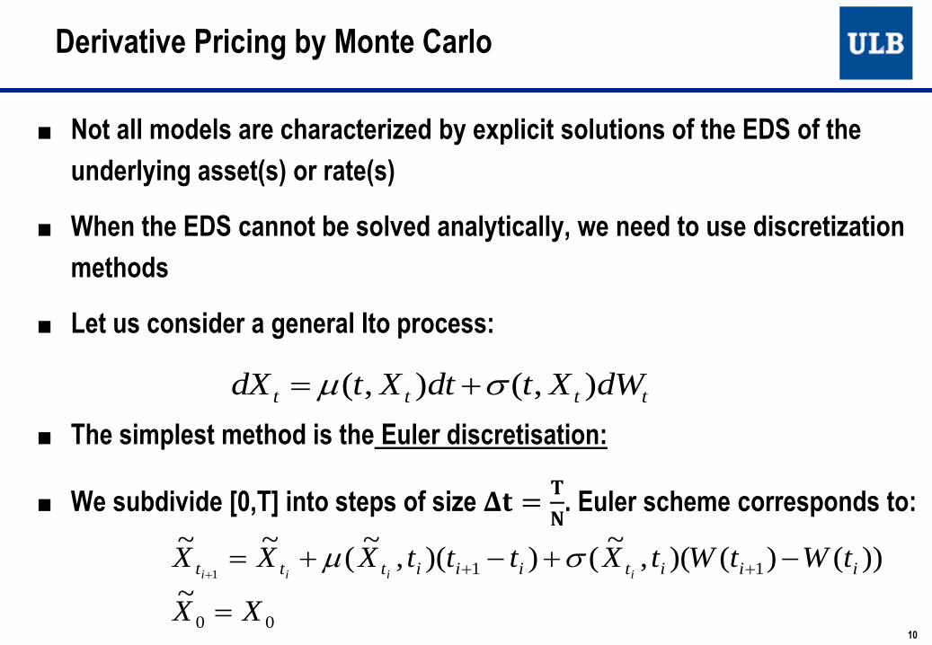
■ Not all models are characterized by explicit solutions of the EDS of the

underlying asset(s) or rate(s)

■ When the EDS cannot be solved analytically, we need to use discretization

methods

■ Let us consider a general Ito process:

■ The simplest method is the Euler discretisation:

■ We subdivide [0,T] into steps of size 𝚫𝐭 =𝐓

𝐍. Euler scheme corresponds to:


00

11

~

))()()(,~

())(,~

(~~

1

XX

tWtWtXtttXXX iiitiiittt iiii

tttt dWXtdtXtdX ),(),(

11

■ The Euler scheme derives from a simple integration rule and the definition

of the Ito integral

■ One can show that this scheme converges in 𝑳𝟐 to the solution of the

EDS, in the following sense:

∃𝑪 > 𝟎 𝒔. 𝒕. 𝑬 𝑿𝒕𝒌 − 𝑿 𝒕𝒌𝟐≤ 𝑪𝚫𝐭 ∀𝒌 ∈ {𝟎, 𝟏, … ,𝑵 − 𝟏}

(Maruyama, 1955)


)(),()(),(:

),(),(),(:

)(),(),(

1

11

11

1

iit

t

tt

iit

t

tit

t

tt

t

tt

t

tttt

tWtXtdWtXand

ttXdttXdttXwhere

tdWtXdttXXX

i

i

i

i

i

ii

i

i

i

i

i

iii

12

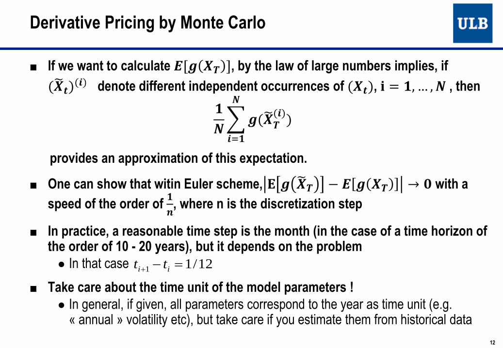
■ If we want to calculate 𝑬[𝒈 𝑿𝑻 ], by the law of large numbers implies, if

(𝑿 𝒕)(𝒊) denote different independent occurrences of (𝑿𝒕), 𝐢 = 𝟏,… ,𝑵 , then

𝟏

𝑵 𝒈(𝑿 𝑻

(𝒊))

𝑵

𝒊=𝟏

provides an approximation of this expectation.

■ One can show that witin Euler scheme, 𝐄 𝒈 𝑿 𝑻 − 𝑬 𝒈 𝑿𝑻 → 𝟎 with a

speed of the order of 𝟏

𝒏, where n is the discretization step

■ In practice, a reasonable time step is the month (in the case of a time horizon of the order of 10 - 20 years), but it depends on the problem

● In that case

■ Take care about the time unit of the model parameters !

● In general, if given, all parameters correspond to the year as time unit (e.g. « annual » volatility etc), but take care if you estimate them from historical data

12/11 ii tt


13

■ Milstein scheme improves this discretization if 𝝁 and 𝝈 do not

depend on time

■ It is based on a Taylor development of 𝝈(𝒙) (based on Ito lemma)

■ It consists to the following approximation

■ One can show that the scheme converges a.s. and in 𝑳𝟐, with a

greater speed than the Euler scheme

))()(~

()~

(5.0

)()~

()~

(~~

2

1

iitt

itittt

ttWXdx

dX

tWXtXXX

ii

iiii


14

► Idea of the derivation of Milstein scheme:

► (source: J. Palczewski, course computation in finance, Uni. Leeds):


15

► Idea of the derivation (continued):



16

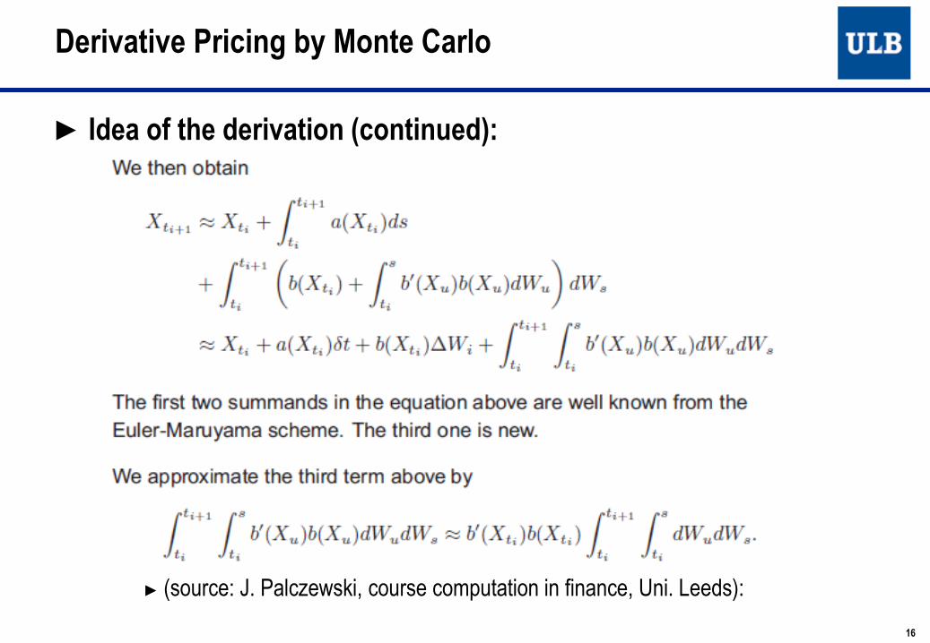
► Idea of the derivation (continued):



17

■ One can also accelerate convergence

● Ex: “antithetic variates” within Euler scheme:

● In practice, within a pricing tool: One generates only ONE set of random numbers 𝜖𝑖 ∼ 𝑁(0,1) per

simulation path

BUT cash-flows (payoffs) are projected along the TWO sets of simulation paths in parallel

Consider then for each couple of simulated path (with the “+” and with the “-” but the same 𝜖𝑖 ) the average payoff(s)

The result is finally a simple set of simulated payoffs, from which we take the mean

iiiitiiittt

iiiitiiittt

tttXtttXXX

tttXtttXXX

iiii

iiii

11

11

),())(,(

),())(,(


■ In practice, options might involve also (risk-free) interest rates

■ In that case, we work in a stochastic framework for interest rates, and we will see that the general pricing formula becomes:

■ where r(s) denotes the short rate at time s (see later)

■ Monte Carlo pricing becomes hence:


18

it

t

N

i

iQ dssrtpayoffEtP )(exp)()(1

NbSimul

scen

scen

N

i

iscen

NbSimul

scen

i

k

iiscen

N

i

iscen

DFstotpayoffNbSimul

ttrtpayoffNbSimul

tP

1 1

1 1

1

1

)(1

))(exp()(1

)(

19

Simulations Basics about pseudo-Random Numbers Generation

In order to perform the Monte-Carlo simulation of the processes by

discretization (Euler or other), we need to be able to generate pseudo-

random numbers

Example: if = 1/12 (1 month), if projection horizon N = 20 years, 240 independent

generations by scenario are required

for 10000 generated scenarios, this leads to 2 400 000 random numbers by Brownian motion present in an ESG

we need to have a pseudo-random numbers generator with a sufficient cycle

Pre-programmed function in numerical software like Matlab, SAS, R are in general sufficient for option pricing: rand, random, ranuni,… It is important however to pay attention to their cycle, depending on the number of factors

It is becoming insufficient if about 109 simulations of random numbers are required

ii tt 1

19

20

■ The first step is to construct pseudo-random numbers following a uniform law on [0,1]

■ A well-known method consists to use congruential generators

■ Simple linear congruential generators:

● The idea is to choose huge integers a, c, m , and to generate pseudo-random numbers by:

for a choice of initial seed x1.


20

m

xu

mcaxx

ii

ii

11

1 mod)(

21

Some conditions on the numbers a, c, m guarantee that the generator

will generate a complete cycle: “Complete cycle” means that for any choice of initial seed, the m-1 subsequent

generated numbers will all be different

If c≠0, sufficient conditions are given by: c and m are relatively prime

Any prime number dividing m also divides a

a – 1 is divisible by 4 if m also is

If now c=0 and if m is prime, a complete cycle can be generated for any

seed x1≠0 if: am-1 – 1 is a multiple of m

aj-1 – 1 is not a multiple of m for any 𝒋 = 𝟏, … ,𝒎 − 𝟐

21


22

In practice, a well known congruential generator corresponds to:

m = 231 – 1 = 2147483647, a = 16807, c=0

(Park-Miller generator)

Remark: this choice of m corresponds to the greatest integer that can be

stored in a 32 bits computer

1 bit for the sign 31 bits for the digits in a binary basis,

This was important in the past when deciding to work with variables

declared in the “long integer” type and not with the “double [precision]”

type, which was more efficient in terms of computational speed

22


23

Other possibilities are given by:

m a

231 – 1

(= 2 147 483 647)

16 807

39 373

742 938 285

950 706 376

1 226 874 159

2 147 483 399 40 692

2 147 483 563 40 014

23


24

In practice, as the sequence of generated numbers can be arbitrarily close to e m,

by multiplying these by a during the generation, we arrive always to an over-flow if

we work with an “integer” type in order to avoid overflows, it is possible to decompose m into:

m=a q + r, where r = m mod a.

In that case, we use the fact that

and that the second term above is always equal to m or 0

As the result is between 0 and m-1, we are sure that the last term is equal to m only

if :

mm

ax

q

xr

q

xqxamax iii

ii

)mod(mod

.0)mod(

r

q

xqxa i

i

24


25

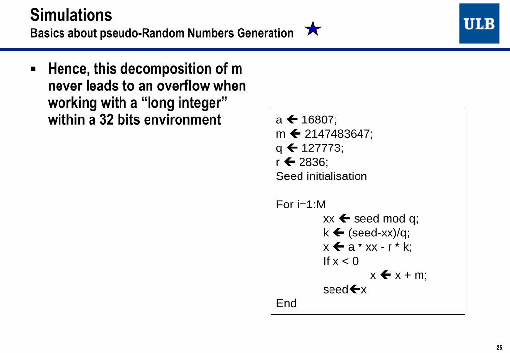
Hence, this decomposition of m never leads to an overflow when working with a “long integer” within a 32 bits environment

a 16807;

m 2147483647;

q 127773;

r 2836;

Seed initialisation

For i=1:M

xx seed mod q;

k (seed-xx)/q;

x a * xx - r * k;

If x < 0

x x + m;

seedx

End

25


26

Other methods have been developped and are used (ex: multiple congruential…)

References:

● Glasserman, P., Monte Carlo Methods in Financial Engineering, Springer-Verlag, New

York (2004).

● L’Ecuyer,P. Efficient and portable combined random number generators, Communications

of the ACM 31, 742-749, Correspondence 32, 1019-1024 (1988).

● L’Ecuyer,P., Good parameters and implementations for combined multiple recursive

random number generators, Operations Research 47, 159-164 (1999).

● Knuth, D.E., The art of computer programming, Volume II: Seminumerical Algorithms,

Third Edition, Addison Wesley Longman, Reading, Mass (1998).

● Fishman, G.S., Monte Carlo: concepts, algorithms, and applications, Springer-Verlag,

New York (1996).

26


27

Simulations Generation of standard normal numbers (1/4)

We need to generate numbers εi following standard normal distributions

N(0,1)

The first step is to generate independent realisations of standard normal

distributions

Several methods can be considered. One of these: Polar rejection method.

Generate two numbers following independent uniform laws on [-1, 1]:

u1 , u2

Calculate w = (u1)² + (u2)², and if w<1, set:

e1=( -2 ln(w)/w )1/2 u1

e2=( -2 ln(w)/w )1/2 u2

If 𝒘 ≥ 𝟏, reject the couple (u1 , u2 ) and generate another couple

27

28

Alternative method: Box-Muller:

𝑹 = −𝟐 𝒍𝒏(𝒖𝟏)

𝑾 = 𝟐𝝅𝒖𝟐

𝒆𝟏 = 𝑹 𝒄𝒐𝒔(𝑾) 𝒆𝟐 = 𝑹 𝒔𝒊𝒏(𝑾)

This method is linked to the choice of polar coordinates and to the

fact that if Z=(Z1,Z2 )~N(0,Id) is a bivariate Gaussian vector, then:

𝑹 = 𝒁𝟏² + 𝒁𝟐

² ~ Exponential distribution with mean 2

Conditionally to R, the vector (Z1,Z2) follows a bivariate uniform distribution (with

independent margins) on the circle of radius 𝑹 centered at the origin

28


e2

e1

R1/2

29

Other method: direct inversion of the cumulative distribution function Ф of the standard normal N(0,1)

No analytical expression of Ф in terms of elementary functions (exp, log, sin, cos, polynomials,…).

Approximation of the inverse of Ф:

5.00)1()(

192.0))1ln(ln()(

92.05.0)5.0(1

)5.0()(

11

8

0

1

3

0

2

3

0

12

1

uuu

uucu

uub

uau

n

n

n

n

n

n

n

n

n

29


30

where:

3736090038405729.0

3151870000003960.03338630276438810.0

1673640000002888.09182091607979714.0

8817680000321767.09171869761690190.0

5119190003951896.07261473374754822.0

31308290983.374410604963.25

60622410182.2143911977353.41

30833674374.2396150006252.18

04735109309.845066282388.2

4

83

72

61

50

33

22

11

00

c

cc

cc

cc

cc

ba

ba

ba

ba

30


31

■ This becomes important in option pricing for basket options, or options depending on several underlying variables

■ The different variables are generally dependent

■ A simple possibility is to incorporate linear correlations between the different Brownian motions of the different processes

■ In practice: Cholesky decomposition

● At the level of the pseudo-random numbers generated following N(0,1)

● Correlation levels need of course to be estimated, like any other parameter

■ First step: Generation of the independent numbers εi, one sequence of numbers by Brownian motion, and introduction of correlations between the different sequences

Simulations Dependencies between the different variables

31

32

Simulations Introduction of correlations between Brownian motions (1/4)

• Cholesky decomposition: decomposition of the correlation matrix in a

product of an upper and a lower triangular matrices

• As the correlation matrix ρ is symmetric, on can show that there exists a

lower triangular matrix L such that LLT =ρ.

• We then use the following result:

• If 𝒁 = (𝒁𝟏, … , 𝒁𝒅) is a vector of independent Gaussian variables, if 𝑳𝑳𝑻 = 𝝆,

then 𝑾 = 𝑳𝒁𝑻 is a Gaussian vector with correlation matrix 𝝆

• Thanks to this result, it suffices to find L, and to multiply the Gaussian

vectors (obtained by using one of the previous method for generating

i.i.d. Gaussian numbers) corresponding to the same simulation instant

by the matrix L

32

33

In practice, the first step is to find the matrix L of the Cholesky decomposition

● The algorithm corresponds simply to write the equation LLT =ρ on an element by element basis:

and isolate in a member of the equation L(k=i,j) (first treat the case i=j ,

then the case i>j)

),(),(),(),(),(1

jijkLikLiiLjiLn

ikk


33

34

This leads to the following algorithm:

for i=1:N

for j=1:N

A(i,j)=0;

end

end

for j=1:N

for i=j:N

V(i)=correl(i,j);

for k=1:(j-1)

V(i)=V(i)-A(j,k)*A(i,k);

end

A(i,j)=V(i)/sqrt(V(j));

end

end

resultat=A;


34

35

► The correlations are then introduced between the numbers εi (we suppose here that we have M Brownian motions) by a loop::

j

k

jkcorr kiMLjiMj1

))1((),( :...1For

where i represents a given instant in a given generated scenario

The index i is used later within the generation of the process associated to one

asset or variable by Euler (or variant) discretisation scheme, for the increase of

Brownian motion for the jth process).

In practice:

One considers groups of M numbers generated following standard Gaussian

variables, and we introduce correlations within each group

At a given instant in a given scenario, the M numbers εcorr(i,j) correspond to

realisations of variables that are correlated with the correlation matrix ρ.


35

36

Vasicek model - Euler discretisation:

where εi are normal variables N(0,1) i.i.d.

Now, in the case of Vasicek model, some alternative discretization schemes exist, deduced from the explicit expression of the short rate

⇒ 𝑟𝑡 = 𝑟0 exp −𝑘𝑡 + 𝜇 1 − exp −𝑘𝑡 + 𝜎 exp −𝑘(𝑡 − 𝑢) 𝑑𝑊𝑢𝑡

0

The same methodology can be applied for Hull-White model from the explicit solution for the short rate

iiiiiiitt tttttartrrii

11 )))(()((1

)())()(()( tdWdttarttdr

36

k

tktktktrttr

tdWdttrktdr

t2

)2exp(1)exp(1()exp()()(

)())(()(

Derivative Pricing by Monte Carlo Interest rates models – Vasicek and Hull – White

37

This can also be applied for the formulation of Hull-White of the form

“Vasicek + deterministic function” previously introduced:

In the case of G2++, the Vasicek schemes for x(t) and y(t) lead to the

following discretization:

)²1(²2

),0()(

)()()(

)()()(

2atM e

atft

tdWdttaxtdx

ttxtr

37

)()()()( iiii ttytxtr

),(

2

)2exp(1')exp()()(

2

)2exp(1)exp()()(

'

1

1

ii

iii

iii

corr

b

tbtbtyty

a

tatatxtx


■ Euler scheme:

■ In theory, the probability to get negative rates is zero if Φ(t) >0. The probability

that x(t) reaches 0 is generally 0 as well, but discretisation errors can imply in

practice that we reach the origin and even cross it

■ In order to avoid such a situation, one can replace in the square root the term

x(ti) by its positive value, and by forcing negative values of x(t) to 0, i.e. using

the following modified Euler scheme:

■ An alternative discretisation scheme is due to Scott (cf. references in

[Glassermann, pages 120-124]). The method is summarized below.

iiiiiiiii tttxtttxktxtx

111 ))(()))((()()(

iiiiiiiii tttxtttxktxtx 111 )()))((()()(

0)( 1 itx

then,0)( if 1 itx

38


■ The distribution of r(t) given r(s) for s<t is known explicitly, and appears as a non central chi-square distribution. This property is used to simulate the process.

■ The transition law of the CIR factor x(t) is indeed given by:

stsxe

ke

k

etx

stk

utk

d

stk

,)()1²(

4'

4

)1²()(

)(

)(2

)(

²

4 where

kd

parameter centralitynon with

ondistributi squared chi noncentral a is )( and 2'

d

39

Derivative Pricing by Monte Carlo Interest rates models – CIR++

Now, in order to simulate a noncentral chi-square variable with noncentrality parameter λ

and with an integer ν>1 degrees of freedom, we first can decompose this variable in an

ordinary (i.e. centered) chi-square variable and an independent normal. This can also be

generalised in the case ν is not an integer

Now, if ν>0, by using the definition of a chi-square distribution with a non integer number

of degrees of freedom, we can represent any noncentral chi-square variable with

noncentrality parameter λ as an ordinary (i.e. central) chi-square variable with a random

degrees of freedom parameter, where this stochastic parameter follows actually a

Poisson distribution with mean λ/2

The method consists hence in this case to simulate a central variable where N is a

Poisson distribution

In clear, if ν>1, the variable is simulated as , where Z is a normal

distribution, and if ν is smaller or equal to 1, as where N is a Poisson variable with mean

λ/2

2

2N

2

1)²( Z2'

40


■ Illustration of both discretization methods:

● Averages on simulations of the short rate, 5 and 10 years zero-coupon

rates and theoretical mean (dame parameters). Right: alternative method,

left: standare Euler scheme. Only 1000 simulations (insufficient for a good

convergence towards the theoretical mean).

● The main interesting property of this simulation algorithm is that we avoid

now negative rates when they should in theory not appear

0 50 100 150 200 250 300 350 4000.025

0.03

0.035

0.04

0.045

0.05

0.055Rates comparison (RN scenarios, averages)

Short rate (theor. mean)

Short rate

10 Y ZC rate

5 Y ZC rate

0 50 100 150 200 250 300 350 400 450 5000.025

0.03

0.035

0.04

0.045

0.05Rates comparison (RN scenarios, averages)

Short rate (theor. mean)

Short rate

10 Y ZC rate

5 Y ZC rate

41


introduction to derivative pricing by monte carlohomepages.ulb.ac.be/~cazizieh/levy_files/mc...

Documents