exotic option: pricing path-dependent single barrier option

Exotic Options: Pricing Path-Dependent single Barrier Option contracts

Abukar M Ali Mathematics and Statistics Department

Birkbeck, University of London

© YieldCurve.com of 28

Abstract

This paper discusses the basic properties of barrier options and an analytical solution for pricing such contracts. The significance of monitoring is considered, for example the difference between continuous monitoring and discrete monitoring. Pitfalls arising from a naïve application of standard option valuation techniques to barrier options are pointed out. We also discuss the practical issues related to barrier options, such as the advantages they provide to the buyer as well as to the writer, and consider practical issues behind valuation. Key words and phrases: Barrier Options, Knock-out Options, Knock-in Options, Rebate, Path-dependant Payoff, Black & Scholes, restricted density, Reflection Principal.


1. Introduction Barrier options are a class of exotic options which were first priced by Merton (1973). The most common approaches used to price these type of derivatives are the expectations methods and the differential equation methods. The expectations method has been worked out in detail by Rubinstein and Reiner (1991) and also Rich (1994). The expectations pricing method requires the determination of the risk-neutral densities of the underlying price as it breaches the barrier from above and below. If rebates apply then the first exit time densities through the barrier are also required. Barrier option prices are then obtained, in the usual way, by integrating the discounted barrier option pay-off function over the calculated densities. It is considered difficult to work out these densities when using the expectation approach, it is however remarkable that closed form solutions for all types of barrier options are in fact obtained. A brief discussion of the differential equation method can be found in Wilmott (1993). The basic idea of this approach is that all barrier options satisfy the Black-Scholes partial differential equation but with different domains, expiry conditions and boundary conditions. In principal, these partial differential equations (PDE's) can be transformed to the diffusion equation and solved. Once again the analysis is complex and also requires the evaluation of integrals, but the same closed form solutions are obtained. The solution from the PDE method is of course related to the solutions from the expectation approach. Ritchken (1995) has investigated computational aspects of barrier option pricing using binomial and trinomial lattice. In this paper, the PDE method will be adopted to show that a direct and simple analysis leads to the closed form solutions. The method employs symmetry properties of the Black-Scholes (B&S) PDE and requires little more than the well-known basic European vanilla option solutions. 2. Pricing of simple contingent claims 2.1 Asset Price Dynamics and Ito Process The dynamics of stock price S are represented by the following Ito process with a drift rate of Sµ and variance rate of : 22Sσ

SdXSdtdS σµ += (1.1) divide both sides by S, to obtain the following stochastic differential equation (SDE): dXdtSdS σµ +=/ (1.2) This process of stock prices, known also as the geometric Brownian motion, can be written in discrete time setting as

dttSS ∆+∆=∆ σεµ/ (1.3)


Where ε is a random sample from distribution with zero mean and a unit standard deviation. If we set 0=σ , the term involving dX in equation (1.2), would drop out and we are left with ordinary differential equation (ODE)

dtSdS µ=/ or SdtdS µ=/

Where µ is constant this can be solved exactly to give exponential growth in the value of the asset, i.e. )](exp[ 00 ttSS −= µ The random term dX from equation (1.2) is known as a Weiner process which has the properties defined below. The model has the stock price growing at a constant rate µ , with random fluctuations superimposed. These fluctuations are proportional to the standard deviation of the asset price and are dependant on standard normal random variable. This type of process is known as Weiner process. Definition 1.1 A stochastic process X is called Weiner process if the following hold.1 1. W(0) = 0 2. The process W has independent increments, i.e. if r < s ≤ t < u then W(u) - W(t) and W(s) -W(r) are independent stochastic variables. 3. For s < t the stochastic variable W(t) - W(s) has a Gaussian distribution ).,0( stN − 4. W has continuous trajectories We can write dX as dtdX φ= where φ is a random variable with and a probability density function given by

)1,0(~N

2

21

21 φ

π

−e , for ∞<<∞− φ (1.4)

Define the expectation operator ξ by

∫∞

∞

−= ,)(21(.)][

2

21

φφπ

ξ φ deFF (1.5)

For any function F, then 0][ =φξ and 1][ 2 =φξ

1 Most authors would use the letter W to associate it with the Weiner process.


It follows that from equation 1.2, the expectation and variance of dS can be written as

dtSdXSdSdSdSVarSdtSdXSdtdS

2222222 ][][][][][][

σσξξξµσµξξ

==−=

=+=

2.2 Ito's Lemma Ito's Lemma is an important result about the manipulation of random variables. While Taylor's theorem allows one to manipulate functions of deterministic variables, Ito's Lemma can be applied to manipulate functions of random variables. It relates the small change in a function of random variable to the small change of in the random variable itself. We will use the following Ito's multiplication table2 (dX)2 = dt, dt.dX = 0, (dt)2 = 0, If f(S) is a smooth function of S and we vary S by small amount dS, then the function f will also vary amount small amount df. Using the Taylor series expansion we can write the change of the function f as:

...,21 2

2

2

++= dSdS

fddSdSdfdf (1.6)

Since dS is given by equation (1.1), we square it to find that 22 )( SdXSdtdS σµ +=

2222222 2 dtSdtdXSdXS µσµσ ++= (1.7) the first term is the largest for small dt and dominates the other two terms. We are then left with ...2222 += dXSdS σ Since dX2 → dt, .222 dtSdS σ= 2 See Bjork (1998) for technical details of these results.


We now substitute this result and equation 1.1 into 1.6, such that we find:

dtSdS

fdSdXSdtdSdfdf 22

2

2

21)( σσµ ++=

dtSdS

fdSdXdSdfSdt

dSdfdf 22

2

2

21 σσµ ++=

dXdSdfSdtS

dSfdS

dSdfdf σσµ ++= )

21( 22

2

2

(1.8)

This is Ito's Lemma relating the small change in a function of random variable to the small change in the variable itself. The first component of the right hand side equation is deterministic component of the change in the function f and is proportional to dt. The second component is a random component and is proportional to dt. The result (1.8) can be extended to a function of two variable which entails the use of partial derivatives since there are two independent random variables, i.e. S and t. We can expand f(S + dS, t + dt) in a Taylor series about (S, t) to get

...,21 2

2

2

+∂∂

+∂∂

+∂∂

= dSS

fdttfdS

Sfdf

dXSfSdt

tfS

SfS

Sfdf

∂∂

+∂∂

+∂∂

+∂∂

= σσµ )21( 22

2

2

(1.9)

3.1 The Black -Scholes Formulation of Option Pricing We illustrate how to use the riskless hedging principle to derive the governing partial differential equation for the price of European call. The derivation follows the approach used by Black and Scholes in their seminal paper (1973). They made the following assumption in the financial market: (i) trading takes place continuously in time; (ii) the riskless interest r is known and constant over time; (iii) the asset pays no dividend; (iv) there are no transaction costs in buying or selling the asset or the option, and no taxes; (v) there are no riskless arbitrage opportunities; (vi) short selling is permitted and the assets are divisible. Let V(S, t) be the value of an option whose value depends on both S and t. Using Ito's Lemma, equation (1.9), the random walk followed by V can be written


dXSVSdt

tVS

SVS

SVdV

∂∂

+∂∂

+∂∂

+∂∂

= σσµ )21( 22

2

2

(3.1)

If we now construct a portfolio of consisting a long position of the option and a short position of the underlying asset )( ∆− , the value of the portfolio is SV ∆−=Π (3.2) The change in the portfolio in one-time step is dSdVd ∆−=Π

Let; SV∂∂

=∆

Putting (1.1), (3.1) and (3.2) together, the change in the portfolio can be written as

dXSVSdt

tVS

SVS

SVd

∂∂

+∂∂

+∂∂

+∂∂

=Π σσµ )21( 22

2

2

)( SdXSdt σµ +∆−

SdXSdtdXSVSdt

tVS

SVS

SV σµσσµ ∆−∆−

∂∂

+∂∂

+∂∂

+∂∂

= )21( 22

2

2

Since

SV∂∂

=∆

)()21( 22

2

2

dXSVSdt

SVSdX

SVSdt

tVS

SVS

SVd

∂∂

−∂∂

−∂∂

+∂∂

+∂∂

+∂∂

=Π σµσσµ

by simply rearranging the above equation, we have

dttVS

SVdX

SVSdX

SVSdt

SVS

SVSd )

21()()( 22

2

2

∂∂

+∂∂

+∂∂

−∂∂

+∂∂

−∂∂

=Π σσσµµ

The first two terms from the right hand side of the equation cancels each other and the random component in the equation is eliminated. This results in a portfolio whose increments is wholly deterministic:

dtSSV

tVd )

21( 22

2

2

σ∂∂

+∂∂

=Π (3.3)


Note the uncertainty due to dX is cancelled out and u, the premium for risk (return on S), is also cancelled out. Not only that the term Πd has no uncertainty, it is also preference free and not dependant on u, a parameter controlled by investors risk aversion. If the portfolio value is fully hedged, then no arbitrage implies that it myst earn only risk free rate of return. We then have

dtSSV

tVdtr )

21( 22

2

2

σ∂∂

+∂∂

=Π (3.4)

using equation (3.2)

dtSSV

tVdtSVr )

21()( 22

2

2

σ∂∂

+∂∂

=∆−

since

SV∂∂

=∆

dtSSV

tVdtS

SVVr )

21()( 22

2

2

σ∂∂

+∂∂

=∂∂

−

dtSSV

tVdt

SVrSrV )

21()( 22

2

2

σ∂∂

+∂∂

=∂∂

−

dividing both sides by dt and rearranging the equation, we have

SVrSS

SV

tVrV

∂∂

+∂∂

+∂∂

= 222

2

21 σ

finally

021 22

2

2

=−∂∂

+∂∂

+∂∂ rV

SVrSS

SV

tV σ (3.5)

This is the Black-Scholes partial derivative equation and any derivative security whose price depends only on the current value of S and on t, and which is paid for up-front must satisfy the Black-Scholes equation. The most frequent type of partial differential equation in financial problems is the parabolic equation. Equation (3.5) is called backward parabolic since the equation is linear and the signs of these particular derivatives are the same.


The price of particular derivative security is obtained by solving Equation (3.5) subject to the appropriate auxiliary conditions (terminal payoff) for the corresponding derivative security. The solution of the Black-Scholes equation with different auxiliary conditions can then provide valuation formulas for different types of derivative securities. The term dX disappear from the PDE, which means there is no uncertainty. While the stock price evolves in an uncertain manner, when we value derivatives with respect to stock price, this uncertainty no longer exist in the pricing formula for this derivative. The term u which is the expected rate of return on the stock also disappear from the PDE. The expected return is affected by risk preference. The more risk averse the investor, the smaller the expected return. Given that the expected return does not appear in the pricing formula for derivatives, valuation of derivatives in this framework is preference free. The solution to the differential equation is therefore the same in a risk-free world as it is in the real world. Hence, this type of valuation method are often called, risk neutral valuation relationship (RNVR). Application of RNV sets the expected growth rate of stock equal to risk free interest rate, then discount expected payoff of option at risk free rate. There are many solutions to (3.5) that correspond to different derivatives, f , with underlying asset S . In other words, without further constraints, the PDE in (3.5) does not have a unique solution. The particular security being valued is determined by its boundary conditions of the differential equation. In the case of a European call, the value at expiry

)0,(),( ESTSc −= serves as the final condition for the Black-Scholes PDE. 3.2 Lognormal property and stock price process Black-Scholes (1973) assume that there are two fundamental assets: a bond with a price B(.) and a stock with a price S(.). The price of the bond and the stock are assumed to grow as follows for any Tt ≤≤0 : ),exp()( rttB = and

⎭⎬⎫

⎩⎨⎧

+⎟⎠⎞

⎜⎝⎛ −= )(

21exp)0()( 2 twtStS σσµ ,

where r, u, and σ are constants, and w(t) is a standard Brownian motion3. The ratio of S(T) to S(t) can be written:

3 See Harrison (1985) for mathematical details of Brownian motion. Brownian motion is named after the botanist Robert Brown. Brown noticed in 1827 that pollen exhibits random motion when suspended in water. The mathematics of this "Brownian motion" did not come until Bachelier (1900) and Einstein (1905).


⎭⎬⎫

⎩⎨⎧

+⎟⎠⎞

⎜⎝⎛ −=

⎭⎬⎫

⎩⎨⎧

+⎟⎠⎞

⎜⎝⎛ −=

)(21exp)0()(

)(21exp)0()(

2

2

twtStS

TwTSTS

σσµ

σσµ

(⎭⎬⎫

⎩⎨⎧

−+−⎟⎠⎞

⎜⎝⎛ −= )()()(

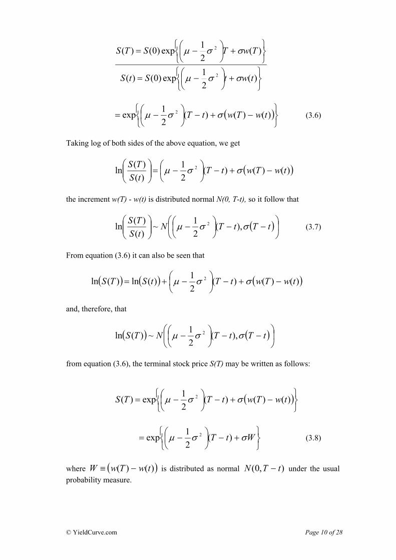
21exp 2 twTwtT σσµ ) (3.6)

Taking log of both sides of the above equation, we get

( ))()()(21

)()(ln 2 twTwtT

tSTS

−+−⎟⎠⎞

⎜⎝⎛ −=⎟⎟

⎠

⎞⎜⎜⎝

⎛σσµ

the increment w(T) - w(t) is distributed normal N(0, T-t), so it follow that

( )⎟⎠

⎞⎜⎝

⎛−−⎟

⎠⎞

⎜⎝⎛ −⎟⎟

⎠

⎞⎜⎜⎝

⎛ tTtTNtSTS

σσµ ),(21~

)()(ln 2 (3.7)

From equation (3.6) it can also be seen that

( ) ( ) ( ))()()(21)(ln)(ln 2 twTwtTtSTS −+−⎟

⎠⎞

⎜⎝⎛ −+= σσµ

and, therefore, that

( ) ( )⎟⎠

⎞⎜⎝

⎛−−⎟

⎠⎞

⎜⎝⎛ − tTtTNTS σσµ ),(

21~)(ln 2

from equation (3.6), the terminal stock price S(T) may be written as follows:

( )⎭⎬⎫

⎩⎨⎧

−+−⎟⎠⎞

⎜⎝⎛ −= )()()(

21exp)( 2 twTwtTTS σσµ

⎭⎬⎫

⎩⎨⎧

+−⎟⎠⎞

⎜⎝⎛ −= WtT σσµ )(

21exp 2 (3.8)

where is distributed as normal ( )()( twTwW −≡ ) ),0( tTN − under the usual probability measure.


As mentioned above the price of European option at time t can be found by discounting the expected payoff of the call option (Where E* denotes expectation taken under the risk-neutral probability measure). The expectation is taken conditional on information at time t [that is, conditional on S(t)]: ( )[ ])()0,)(max)( *)( tSKTSEetc tTr −= −− (3.9) Now, substituting equation (3.8) into (3.9):

.)()()()(

21

)(2

dwwfKetSetc Ww

WtTtTr

+∞+

−∞=

+−⎟⎠⎞

⎜⎝⎛ −

−− ∫ ⎟⎟⎠

⎞⎜⎜⎝

⎛−=

σσµ

(3.9a)

)(wfW is the probability density function (pdf) of w. With ),,0(~ tTNW − it

follows that the probability density function of W is given by

2

21

21)(

⎟⎠⎞

⎜⎝⎛

−−

−= tT

w

W etT

wfπ

Substitute this for in equation (3.9a) to get the call option value: )(wfW

+

∞+

−∞=

+−⎟⎠⎞

⎜⎝⎛ −

−− ∫ ⎟⎟⎠

⎞⎜⎜⎝

⎛−=

w

WtTtTr KetSetc

σσµ )(21

)(2

)()(

x .2

12

21

dwetT

tTw

⎟⎠⎞

⎜⎝⎛

−−

−π

To simplify, let tTw −= ε so that tT

dwd−

=ε and the call option value becomes

επε

εσσµ

deKetSetctTtT

tTr

22

21)(

21

)(

21)()(

−+

∞+

−∞=

−+−⎟⎠⎞

⎜⎝⎛ −

−− ∫ ⎟⎟⎠

⎞⎜⎜⎝

⎛−=

let 0ε be such that 0)())(

21

( 2

=⎟⎠

⎞⎜⎝

⎛ −−+−−

KetStTtTr σεσ

, then

( )⎭⎬⎫

⎩⎨⎧

−⎟⎠⎞

⎜⎝⎛ −−⎟⎟

⎠

⎞⎜⎜⎝

⎛−

= tTrtS

KtT

20 2

1)(

ln1 σσ

ε


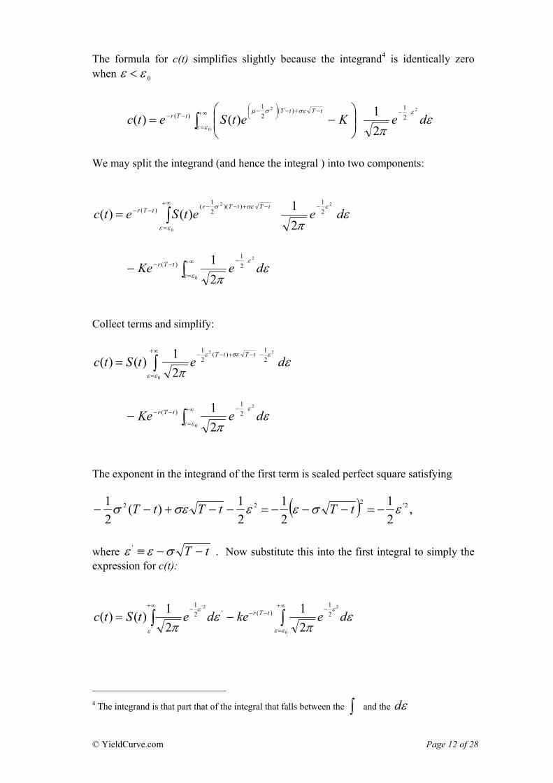
The formula for c(t) simplifies slightly because the integrand4 is identically zero when 0εε <

επ

ε

εε

εσσµ

deKetSetctTtT

tTr2

0

2

21)(

21

)(

21)()(

−∞+

=

−+−⎟⎠⎞

⎜⎝⎛ −

−− ∫ ⎟⎟⎠

⎞⎜⎜⎝

⎛−=

We may split the integrand (and hence the integral ) into two components:

επ

ε

εε

σεσdeetSetc

tTtTrtTr2

0

2

21

))(21

()(

21)()(

−∞+

=

−+−−−− ∫=

∫∞+

=

−−−−0

2

21

)(

21

εε

εε

πdeKe tTr

Collect terms and simplify:

∫∞+

=

−−+−−=

0

22

21)(

21

21)()(

εε

εσεεε

πdetStc

tTtT

∫∞+

=

−−−−0

2

21

)(

21

εε

εε

πdeKe tTr

The exponent in the integrand of the first term is scaled perfect square satisfying

( ) ,21

21

21)(

21 2'222 εσεεσεσ −=−−−=−−+−− tTtTtT

where tT −−≡ σεε ' . Now substitute this into the first integral to simply the expression for c(t):

∫ ∫∞+ ∞+

=

−−−−−=

'0

22'

21

)('21

21

21)()(

ε εε

εεε

πε

πdekedetStc tTr

4 The integrand is that part that of the integral that falls between the and the ∫ εd


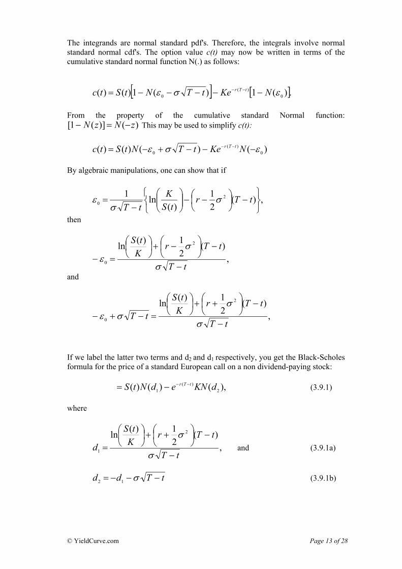
The integrands are normal standard pdf's. Therefore, the integrals involve normal standard normal cdf's. The option value c(t) may now be written in terms of the cumulative standard normal function N(.) as follows: [ ] [ ].)(1)(1)()( 0

)(0 εσε NKetTNtStc tTr −−−−−= −−

From the property of the cumulative standard Normal function:

)()](1[ zNzN −=− This may be used to simplify c(t): )()()()( 0

)(0 εσε −−−+−= −− NKetTNtStc tTr

By algebraic manipulations, one can show that if

,)(21

)(ln1 2

0⎭⎬⎫

⎩⎨⎧

−⎟⎠⎞

⎜⎝⎛ −−⎟⎟

⎠

⎞⎜⎜⎝

⎛−

= tTrtS

KtT

σσ

ε

then

,)(

21)(ln 2

0 tT

tTrKtS

−

−⎟⎠⎞

⎜⎝⎛ −+⎟

⎠⎞

⎜⎝⎛

=−σ

σε

and

,)(

21)(ln 2

0 tT

tTrK

tS

tT−

−⎟⎠⎞

⎜⎝⎛ ++⎟

⎠⎞

⎜⎝⎛

=−+−σ

σσε

If we label the latter two terms and d2 and d1 respectively, you get the Black-Scholes formula for the price of a standard European call on a non dividend-paying stock: (3.9.1) ),()()( 2

)(1 dKNedNtS tTr −−−=

where

,)(

21)(ln 2

1 tT

tTrKtS

d−

−⎟⎠⎞

⎜⎝⎛ ++⎟

⎠⎞

⎜⎝⎛

=σ

σ and (3.9.1a)

tTdd −−−= σ12 (3.9.1b)


The above call price formula can be interpreted using the language of probability. First, is seen as the probability of the call being in-the-money at expiry and so can be interpreted as the risk neutral expectation of the payment made by the holder of the call option at expiry on exercising the option. Second,

is the risk neutral expectation of the asset price at expiry conditional on the call being in-the-money. Hence, the expectation of the call value at expiry is

)( 2dN)( 2dKN

)()( 1)( dNetS tTr −

),()()( 2

)(1 dKNedNtS tTr −−−=

which is then discounted by the factor )( tTre −−= in the risk neutral world to give the present value of the call. 4.1 Barrier Options Options with the barrier feature, commonly called barrier options, are considered to be one of the simplest types of path-dependent options. The unique feature is that the payoff depends not only on the final price of the underlying asset but also on whether or not the underlying asset price has reached (one-touch) some barrier level during the life of the option. An out-barrier option (knock-out option) is one where the option is nullified prior to expiration if the underlying asset price touches the barrier. The option holder may be compensated by a rebate payment for the cancellation of the option. An in-barrier option (knock-in) option is barrier option type which comes into play if the asses price hits or crosses the predefined barrier level. When the barrier is approached from below, the barrier option is called an up-option; otherwise it is called down-option. One can identify eight type of European barrier options, such as down-in calls, up-in calls, down-out calls, up-out calls. And similar four types of options for the European barrier put options. All these options are called standard or vanilla barrier options. The attractiveness of barrier options is that they are cheaper than their corresponding vanilla options, as the sum of the premiums of a knock-in and its corresponding knock-out is always the same as the premium of their corresponding vanilla option if there are no rebates. 4.2 Vanilla barrier options Another name for barrier type options is also a trigger option. This is because the payoff depends critically on whether a pre-specified barrier or a trigger is touched during the life of the option. If the barrier is breached during this time, the holder is entitled to receive a European option. Otherwise, the holder gets a rebate at the maturity of the option. This kind of barrier is known as knock-in barrier option, or simply knock-in. Given the underlying asset price, the barrier level can be placed above of below it. If the barrier is below the underlying price, the knock-in option is called a down knock-in option (DI - for down and in option). The payoff of a down knock-in option (PDI) can be formally given as


[ ] HtSKtSPDI >−= )(|0,)(max{ * ωω

and ,)( HTS ≤ for some },*tTt ≤< (4.2a) or

)(τRmPDI = if S(t) > H and S(T) > H, for all ,*tTt ≤< (4.2b) Where are the current and expiration time of the option respectively; H is the knock-in boundary of the option or the constant barrier level. K is the strike price of the option;

*,, tandt

ω is a binary operator (1 for a call and -1 for a put). )(τRm is the rebate of the barrier option paid at maturity if the barrier is not touched. Below we also so define the payoff for remaining vanilla barrier types such as up-an-in (PUI), down-and-out (PDO). For up-and-out (PUO) payoff see Zhang (1998). The payoff of an up-and-in barrier option (PUI) is given formally as;

[ ] HtSKtSPUI <−= )(|0,)(max{ * ωω and ,)( HTS ≥ for some },*tTt ≤< (4.2c) or

)(τRmPUI = if S(t) < H and S(T) < H, for all ,*tTt ≤< The Payoff of a down and knock out barrier option or simply down-and-out is given; [ ] HtSKtSPDO >−= )(|0,)(max{ * ωω

and ,)( HTS > for some },*tTt ≤< (4.2c) or )(TRPDO = if S(t) > H and S(T) ≤ H, for all ,*tTt ≤< R(T) is in this case also the rebate function which is time dependant. R(T) is most often an increasing function of time starting from zero, or R'(T)> 0 and R(0)=0. The rebate defined in (4.2c) is called non-deferred rebate, implying that the rebate is paid as soon as the barrier is reached. The rebate can also be deferred, that is, the rebate payment can be postponed until maturity.


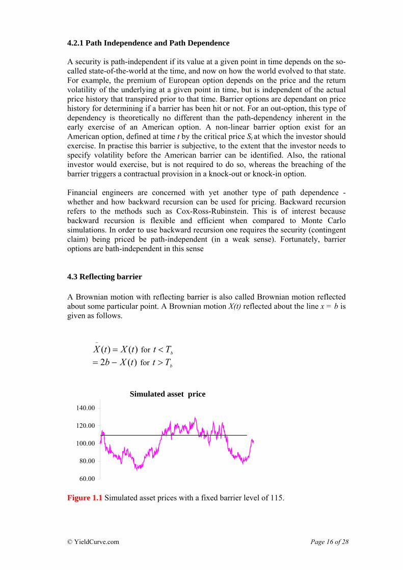
4.2.1 Path Independence and Path Dependence A security is path-independent if its value at a given point in time depends on the so-called state-of-the-world at the time, and now on how the world evolved to that state. For example, the premium of European option depends on the price and the return volatility of the underlying at a given point in time, but is independent of the actual price history that transpired prior to that time. Barrier options are dependant on price history for determining if a barrier has been hit or not. For an out-option, this type of dependency is theoretically no different than the path-dependency inherent in the early exercise of an American option. A non-linear barrier option exist for an American option, defined at time t by the critical price St at which the investor should exercise. In practise this barrier is subjective, to the extent that the investor needs to specify volatility before the American barrier can be identified. Also, the rational investor would exercise, but is not required to do so, whereas the breaching of the barrier triggers a contractual provision in a knock-out or knock-in option. Financial engineers are concerned with yet another type of path dependence - whether and how backward recursion can be used for pricing. Backward recursion refers to the methods such as Cox-Ross-Rubinstein. This is of interest because backward recursion is flexible and efficient when compared to Monte Carlo simulations. In order to use backward recursion one requires the security (contingent claim) being priced be path-independent (in a weak sense). Fortunately, barrier options are bath-independent in this sense 4.3 Reflecting barrier A Brownian motion with reflecting barrier is also called Brownian motion reflected about some particular point. A Brownian motion X(t) reflected about the line x = b is given as follows.

for )()(~

tXtX = bTt < )(2 tXb −= for bTt >

Simulated asset price

60.00

80.00

100.00

120.00

140.00

Figure 1.1 Simulated asset prices with a fixed barrier level of 115.


The well-known result abut the reflecting barrier is the reflection principle which states that for every sample path with X(T) > b there are two sample paths )(TX

and with the same probability of occurrence. Because of the symmetry with respect to b of a Brownian motion

)(~

TX)(tX starting at b, the "probability" of doing this

is the same as the "probability" of travelling from b to the point 2b - X(t). The reason for this is that, for every bath which crosses level b and is found at time t at a point

below b, there is a shadow path obtained from the reflection about the level b which exceeds this level at time t, and these two paths have the same probability. The actual probability for the occurrence of any particular path is zero. With the argument stated above, we can write the equation of the reflection principle as follows:

)(~

tX

[ ] [ ] [ ],)()(,)(, btXPbtXtTPbtXtTP bb >=><=<< Where stands for the time when the reflecting barrier b is first touched and P is the probability. The reflection principle can be used to find the first passage time. The solution of the density functions for the Brownian motion with a reflecting barrier can be found in several text books in financial mathematics

bT

5. 4.4.1 Unrestricted distribution and absorbing barrier Let g stand for the annual continues dividend yield on the underlying asset. The stochastic process which governs the underlying asset price movement given in (1.1) becomes ),()( tSdzSdtgdS σµ +−= where all the parameters are the same as equation (1.1) except for incorporating the continues dividend payout. The solution to the above SDE is given below [ ],)(exp)( τσττ wvSS += where ,* tt −=τ [ ]*,tt stand for current time and expiration time of the option, respectively, ,2/2σ−−= grv and )(τw is standard Gauss-Weiner process (note here that we have changed the notation slightly). We know that [ )/)(ln SSX ]ττ = is the log-return of the underlying asset, then the

density function of is normally distributed with mean τX τv and variance .2τσ its pdf is then given by:

5 For example, see: Yue-Kuen Kwok, Mathematical Models of Financial Derivatives (1998) Also, see: Peter James, Option Theory (2003)


.2

)(exp21)( 2

2

⎥⎦

⎤⎢⎣

⎡ −−=

τστ

πτσvxxf (4.2.1)

Below we provide the result from Cox and Miller (1965) for the density function of a Brownian process with an absorbing barrier. An absorbing barrier is a barrier which upon touching, all the particles vanish.

.2

)(exp21)( 2

2

⎥⎦

⎤⎢⎣

⎡ −−=

τστ

πτσvxxf

⎥⎦

⎤⎢⎣

⎡ −−−−

τστσ

2

2/2

2)2(exp

2 vaxe av for x < a, (4.2.1a)

4.4.2 Restricted Distributions From the specification of the payoff of a brier option, we know that in order to price it, we certainly need another density function conditioned on whether the barrier is reached during the life of the option. Define: [ ]{ },,|)(max ** ttssSM t

t ∈= (4.3a) and [ ]{ },,|)(min ** ttssSmt

t ∈= (4.3b) where Xx∈ stands for that x belongs to X; [ ]*,tt stands for the set of real numbers starting from t and ending at t* . max and min represent the functions giving the maximum and the minimum of a set of numbers, respectively. The two variables given in (4.3a) and (4.3b) are the maximum and minimum of all underlying asset prices within the life of the option. We can express these in terms of log-returns: and (4.3c) )/ln( * SMY t

t=τ )/ln( * SMy tt=τ

let stand for the time the underlying asset price first reaches an up barrier U. The following always hold:

aT


),()()( * aYPUMPTP rttrar <=<=> ττ (4.4a)

and ),()()( * aYPUMPTP r

ttrar ≥=≥=≤ ττ (4.4b)

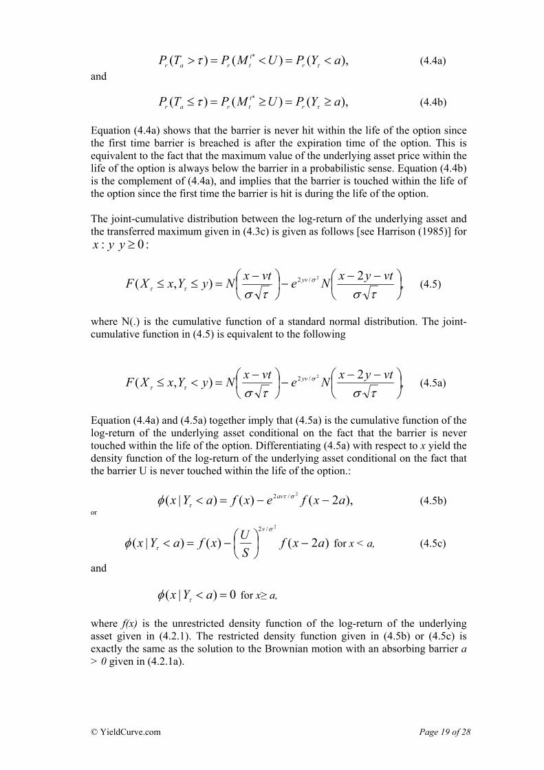
Equation (4.4a) shows that the barrier is never hit within the life of the option since the first time barrier is breached is after the expiration time of the option. This is equivalent to the fact that the maximum value of the underlying asset price within the life of the option is always below the barrier in a probabilistic sense. Equation (4.4b) is the complement of (4.4a), and implies that the barrier is touched within the life of the option since the first time the barrier is hit is during the life of the option. The joint-cumulative distribution between the log-return of the underlying asset and the transferred maximum given in (4.3c) is given as follows [see Harrison (1985)] for

yx : :0≥y

,2),(2/2 ⎟

⎠⎞

⎜⎝⎛ −−

−⎟⎠⎞

⎜⎝⎛ −

=≤≤τστσ

σττ

vtyxNevtxNyYxXF yv (4.5)

where N(.) is the cumulative function of a standard normal distribution. The joint-cumulative function in (4.5) is equivalent to the following

,2),(2/2 ⎟

⎠⎞

⎜⎝⎛ −−

−⎟⎠⎞

⎜⎝⎛ −

=<≤τστσ

σττ

vtyxNevtxNyYxXF yv (4.5a)

Equation (4.4a) and (4.5a) together imply that (4.5a) is the cumulative function of the log-return of the underlying asset conditional on the fact that the barrier is never touched within the life of the option. Differentiating (4.5a) with respect to x yield the density function of the log-return of the underlying asset conditional on the fact that the barrier U is never touched within the life of the option.: (4.5b) ),2()()|(

2/2 axfexfaYx av −−=< σττφ

or

)2()()|(2/2

axfSUxfaYx

v

−⎟⎠⎞

⎜⎝⎛−=<

σ

τφ for x < a, (4.5c)

and 0)|( =< aYx τφ for x≥ a, where f(x) is the unrestricted density function of the log-return of the underlying asset given in (4.2.1). The restricted density function given in (4.5b) or (4.5c) is exactly the same as the solution to the Brownian motion with an absorbing barrier a > 0 given in (4.2.1a).


The complement of being always below the barrier is not always being above or at the barrier, because it is possible that the barrier is reached and the price ends up below. The density function that the barrier is touched can be obtained from the following identity. )()|()|( xfaYxaYx =<+≥ ττ φφ (4.5d) This equation can be interpreted as the summation of the probability when the barrier is touched and the probability when the barrier is never touched within the live of the option, and this is the same as the unrestricted density given in (4.2.1a). 4.5.1 Distribution of the first passage time The first passage time to a particular point on the path of the underlying asset price is the first time that this particular point is first reached. The joint probability that x = y = a > 0 for an up-barrier cab be obtained using (4.4a) and (4.5)

),(),( τ>≤=≤≤ attt TaXPaYaXP

,2/2 ⎟

⎠⎞

⎜⎝⎛ −−

−⎟⎠⎞

⎜⎝⎛ −

=τστσ

σ vtaNevtaN av (4.6)

if the drift term ,02/2 ≥−−= σgrv the density function of the first passage time from zero to the transferred barrier point 0)/ln( >= SUa can be obtained by differentiating (4.6) with respect to the time to maturity.

T

aYaXFaTh=

⎥⎦⎤

⎢⎣⎡ ≤≤

∂∂

−=>τ

τττ),()0|(

⎥⎦

⎤⎢⎣

⎡ −−=

TvTa

Ta

2

2

3 2)(exp

2 σπσ (4.6a)

equation (4.6a) is the distribution of the first passage time. 5.1 Pricing standard barrier options One of the oldest barrier option types such as down-and-out call options were first made available in the U.S. market from 1967. The corresponding valuation formula for these options was driven by Merton (1973). A decade later Bergman (1983) developed a framework for pricing path-dependant claims such as barrier options, and Cox and Rubinstein (1985) used their down-and-out formula to price fixed income securities with embedded characters. Rubinstein and Reiner (1991) also contributed detailed results for all barrier option types with the assumption that the underlying asset price follows lognormal process.


The expected payoffs of in and out barrier options can be calculated in the same way as in vanilla options with the only exception that the restricted density function shown above is used. Using a risk-neutral evaluation relationship, one can obtain barrier option prices by discounting the expected payoffs at the risk-free rate of return. The barrier option is however also affected by the relative magnitude of the strike price and the barrier level. For a down-and-in call with a strike price K greater than the barrier level H and without any rebate, the value of the call can be found by integrating the payoff of a vanilla call option with the restricted density function for all possible underlying asset price starting from the strike price K to infinity. If however the strike price is below or lower the barrier, the payoff of the down-and-in call barrier option includes two parts: the integration of the payoff function of a vanilla call option with the restricted density functions given in (5.1a) for all possible underlying asset prices starting from the barrier H = L to infinity, and the integration of the same payoff function with the density function given in (5.1b) for all S starting from the strike price K to the barrier H = L.

)2()2()|(2

2/2

/ axfSLbxfebYx

vbv −⎟

⎠⎞

⎜⎝⎛=−=≤

σσ

τφ for x > b (5.1a)

and )()|( xfbYx =≥τφ for x ≤ b, (5.1b) where b = ln(L/S) and L stands for a down-barrier L < S. (5.1a) is the restricted density function of the underlying asset log-return under the condition that the down-barrier is touched within the options lifetime. 5.2 Down-and-in barrier call option The payoff of a down-an-in barrier call option can be divided in two parts; one part including the payoff of the corresponding vanilla option if the barrier is reached any time within the life of the option, and the rebate if the barrier is never reached. Within the life of the option. Lets first consider the case where the strike is greater than the barrier level ( K > H ). The value of down-and-in call option (VDIC) without any rebate if the barrier is reached is readily obtained by discounting it is expected payoff given in equation (4.2a) at the risk-free rate of return:

,,,22

1

2/2 2

⎪⎭

⎪⎬⎫

⎪⎩

⎪⎨⎧

⎥⎦

⎤⎢⎣

⎡⎟⎠

⎞⎜⎝

⎛−⎥

⎦

⎤⎢⎣

⎡⎟⎠

⎞⎜⎝

⎛⎟⎠

⎞⎜⎝

⎛⎟⎠⎞

⎜⎝⎛= −− K

SHdNKeK

SHdNe

SH

SHVDIC bs

rbs

gv

ττσ

where


,)/ln()2/()/ln(),(2

τστ

τστσ vKSgrKSKSdbs

+=

−−+=

τσ+= ),(),(1 KSdKSd bsbs

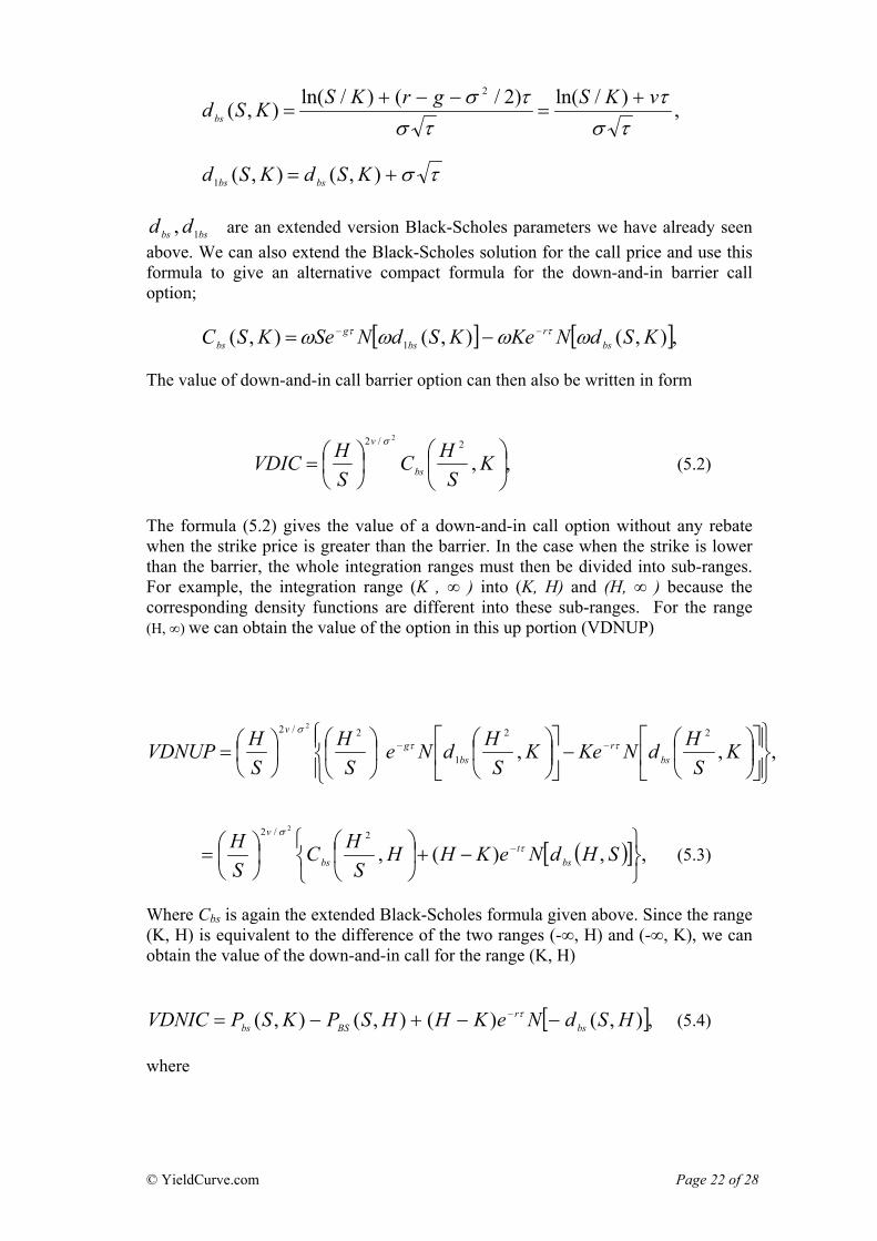
bsbs dd 1, are an extended version Black-Scholes parameters we have already seen above. We can also extend the Black-Scholes solution for the call price and use this formula to give an alternative compact formula for the down-and-in barrier call option;

[ ] [ ],),(),(),( 1 KSdNKeKSdNSeKSC bsr

bsg

bs ωωωω ττ −− −= The value of down-and-in call barrier option can then also be written in form

,,2/2 2

⎟⎠

⎞⎜⎝

⎛⎟⎠⎞

⎜⎝⎛= K

SHC

SHVDIC bs

v σ

(5.2)

The formula (5.2) gives the value of a down-and-in call option without any rebate when the strike price is greater than the barrier. In the case when the strike is lower than the barrier, the whole integration ranges must then be divided into sub-ranges. For example, the integration range (K , ∞ ) into (K, H) and (H, ∞ ) because the corresponding density functions are different into these sub-ranges. For the range (H, ∞) we can obtain the value of the option in this up portion (VDNUP)

,,,22

1

2/2 2

⎪⎭

⎪⎬⎫

⎪⎩

⎪⎨⎧

⎥⎦

⎤⎢⎣

⎡⎟⎠

⎞⎜⎝

⎛−⎥

⎦

⎤⎢⎣

⎡⎟⎠

⎞⎜⎝

⎛⎟⎠

⎞⎜⎝

⎛⎟⎠⎞

⎜⎝⎛= −− K

SHdNKeK

SHdNe

SH

SHVDNUP bs

rbs

gv

ττσ

( )[ ,,)(,2/2 2

⎭⎬⎫

⎩⎨⎧

−+⎟⎠

⎞⎜⎝

⎛⎟⎠⎞

⎜⎝⎛= − SHdNeKHH

SHC

SH

bst

bs

vτ

σ

] (5.3)

Where Cbs is again the extended Black-Scholes formula given above. Since the range (K, H) is equivalent to the difference of the two ranges (-∞, H) and (-∞, K), we can obtain the value of the down-and-in call for the range (K, H)

[ ],),()(),(),( HSdNeKHHSPKSPVDNIC bsr

BSbs −−+−= − τ (5.4) where


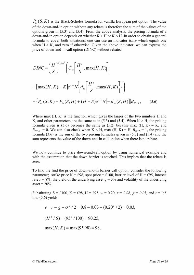
),( KSPbs is the Black-Scholes formula for vanilla European put option. The value of the down-and-in option without any rebate is therefore the sum of the values of the options given in (5.3) and (5.4). From the above analysis, the pricing formula of a down-and-in option depends on whether K > H or K < H. In order to obtain a general formula to cover both situations, one can use an indicator BH>K which equals one when H > K, and zero if otherwise. Given the above indicator, we can express the price of down-and-in call option (DINC) without rebate:

⎜⎜⎝

⎛⎥⎦

⎤⎢⎣

⎡⎟⎠⎞

⎜⎝⎛= ),max(,

2/2 2

KHS

HCSHDINC bs

v σ

[ ] ⎟⎟⎠

⎞

⎭⎬⎫

⎩⎨⎧

⎥⎦

⎤⎢⎣

⎡−+ − ),max(,),max(

2

KHS

HdNeKKH bsrτ

[ ]{ } ,),()(),(),( KHbs

rbsbs BHSdNeSHHSPKSP >

− −−+−+ τ (5.6) Where max (H, K) is the function which gives the larger of the two numbers H and K, and other parameters are the same as in (5.3) and (5.4). When K > H, the pricing formula given is (3.6) becomes the same as (5.2) because max (H, K) = K, and BH>K = 0. We can also check when K < H, max (H, K) = H, BH>K = 1, the pricing formula (3.6) is the sun of the two pricing formulas given in (5.3) and (5.4) and the sum represents the value of the down-and-in call option when there is no rebate. We now continue to price down-and-call option by using numerical example and with the assumption that the down barrier is touched. This implies that the rebate is zero. To find the find the price of down-and-in barrier call option, consider the following parameter; strike price K = £98, spot price = £100, barrier level of H = £95, interest rate r = 8%, the yield of the underlying asset g = 3% and volatility of the underlying asset = 20% Substituting S = £100, K = £98, H = £95, w = 0.20, r = 0.08, g = 0.03, and t = 0.5 into (5.6) yields

,03.0)2/20.0(03.08.02/ 22 =−−=−−= σgrv

,25.90)100/95()/( 22 ==SH

,98)98,95max(),max( ==KH


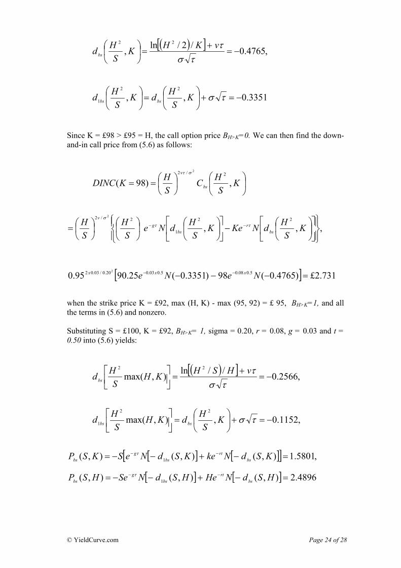
( )[ ] ,4765.0/2/ln,22

−=+

=⎟⎠

⎞⎜⎝

⎛τσ

τvKHKS

Hdbs

3351.0,,22

1 −=+⎟⎠

⎞⎜⎝

⎛=⎟

⎠

⎞⎜⎝

⎛ τσKS

HdKS

Hd bsbs

Since K = £98 > £95 = H, the call option price BH>K=0. We can then find the down-and-in call price from (5.6) as follows:

⎟⎠

⎞⎜⎝

⎛⎟⎠⎞

⎜⎝⎛== K

SHC

SHKDINC bs

v

,)98(2/2 2στ

,,,22

1

2/2 2

⎪⎭

⎪⎬⎫

⎪⎩

⎪⎨⎧

⎥⎦

⎤⎢⎣

⎡⎟⎠

⎞⎜⎝

⎛−⎥

⎦

⎤⎢⎣

⎡⎟⎠

⎞⎜⎝

⎛⎟⎠

⎞⎜⎝

⎛⎟⎠⎞

⎜⎝⎛= −− K

SHdNKeK

SHdNe

SH

SH

bsr

bsg

vττ

σ

[ ] 731.2£)4765.0(98)3351.0(25.9095.0 5.008.05.003.020.0/03.02 2

=−−− −− NeNe xxx when the strike price K = £92, max (H, K) - max (95, 92) = £ 95, BH>K=1, and all the terms in (5.6) and nonzero. Substituting S = £100, K = £92, BH>K= 1, sigma = 0.20, r = 0.08, g = 0.03 and t = 0.50 into (5.6) yields:

( )[ ] ,2566.0//ln),max(22

−=+

=⎥⎦

⎤⎢⎣

⎡τσ

τvHSHKHS

Hdbs

,1152.0,),max(22

1 −=+⎟⎠

⎞⎜⎝

⎛=⎥⎦

⎤⎢⎣

⎡ τσKS

HdKHS

Hd bsbs

[ ] [ ][ ] ,5801.1),(),(),( 1 =−+−−= −− KSdNkeKSdNeSKSP bsrt

bsg

bsτ

[ ] [ ] 4896.2),(),(),( 1 =−+−−= −− HSdNHeHSdNSeHSP bs

rtbs

gbs

τ


⎥⎦

⎤⎢⎣

⎡⎟⎠

⎞⎜⎝

⎛⎟⎠

⎞⎜⎝

⎛=⎟

⎠

⎞⎜⎝

⎛ 95,10095

10095),max(,

2

15.003.0

22

bsx

bs dNeKHS

HC

9816.395,1009595

25.008.0 =⎥

⎦

⎤⎢⎣

⎡⎟⎠

⎞⎜⎝

⎛− −

bsx dNe

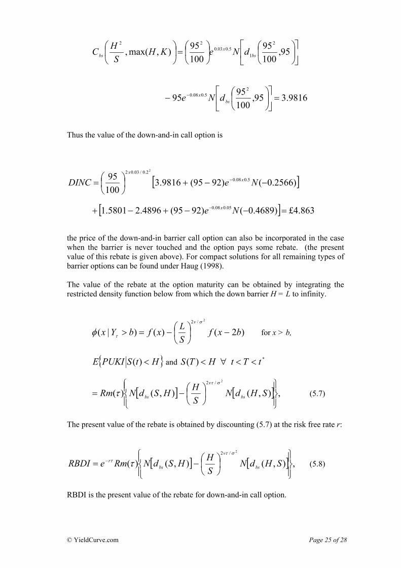
Thus the value of the down-and-in call option is

[ ])2566.0()9295(9816.310095 5.008.0

2.0/03.02 2

−−+⎟⎠⎞

⎜⎝⎛= − NeDINC x

x

[ ] 863.4£)4689.0()9295(4896.25801.1 05.008.0 =−−+−+ − Ne x

the price of the down-and-in barrier call option can also be incorporated in the case when the barrier is never touched and the option pays some rebate. (the present value of this rebate is given above). For compact solutions for all remaining types of barrier options can be found under Haug (1998).

The value of the rebate at the option maturity can be obtained by integrating the restricted density function below from which the down barrier H = L to infinity.

)2()()|(2/2

bxfSLxfbYx

v

−⎟⎠⎞

⎜⎝⎛−=>

σ

τφ for x > b,

{ }HtSPUKIE <)( and HTS <)( ∀ *tTt <<

[ ] [ ] ,),(),()(2/2

⎪⎭

⎪⎬⎫

⎪⎩

⎪⎨⎧

⎟⎠⎞

⎜⎝⎛−= SHdN

SHHSdNRm bs

v

bs

στ

τ (5.7)

The present value of the rebate is obtained by discounting (5.7) at the risk free rate r:

[ ] [ ,),(),()(2/2

⎪⎭

⎪⎬⎫

⎪⎩

⎪⎨⎧

⎟⎠⎞

⎜⎝⎛−= − SHdN

SHHSdNRmeRBDI bs

v

bsr

σττ τ ] (5.8)

RBDI is the present value of the rebate for down-and-in call option.


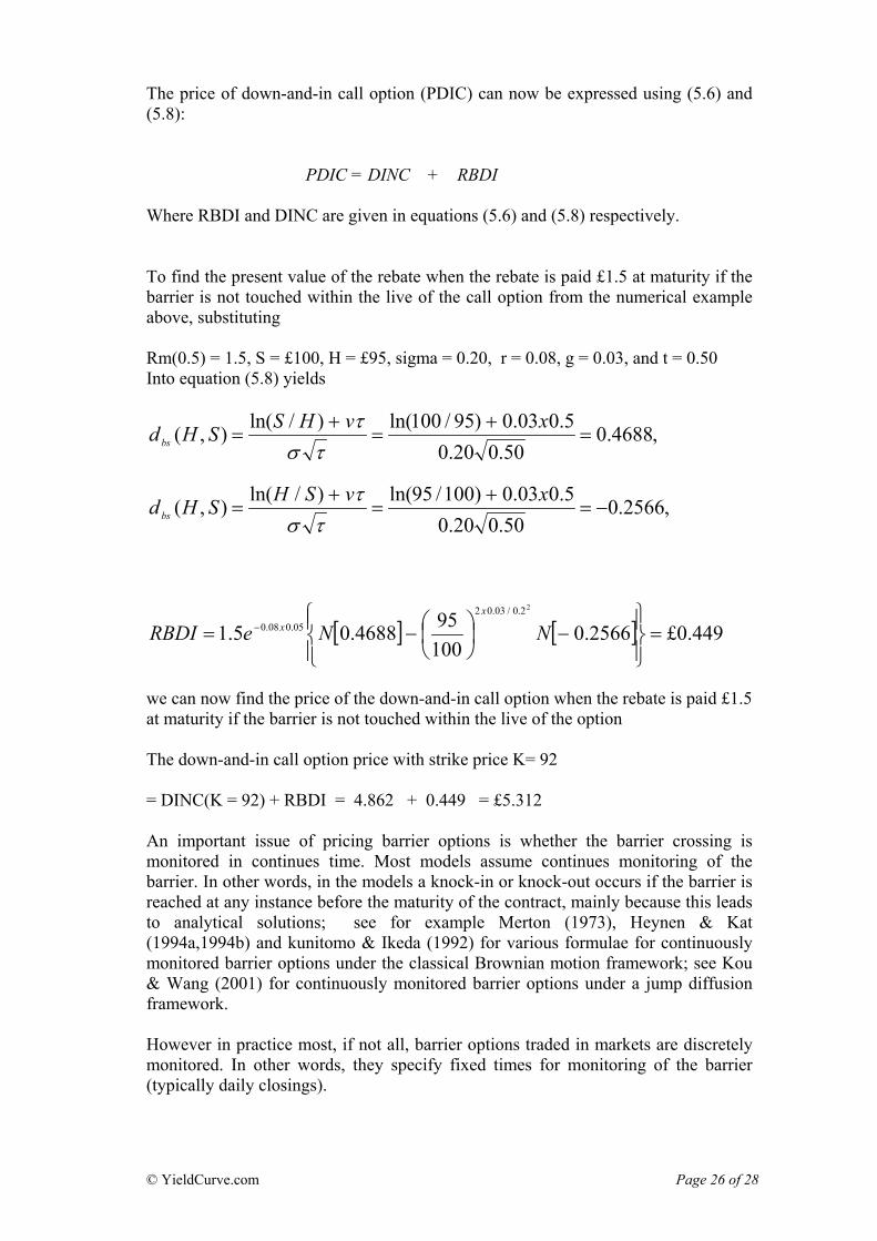
The price of down-and-in call option (PDIC) can now be expressed using (5.6) and (5.8): PDIC = DINC + RBDI Where RBDI and DINC are given in equations (5.6) and (5.8) respectively. To find the present value of the rebate when the rebate is paid £1.5 at maturity if the barrier is not touched within the live of the call option from the numerical example above, substituting Rm(0.5) = 1.5, S = £100, H = £95, sigma = 0.20, r = 0.08, g = 0.03, and t = 0.50 Into equation (5.8) yields

,4688.050.020.0

5.003.0)95/100ln()/ln(),( =+

=+

=xvHSSHdbs τσ

τ

,2566.050.020.0

5.003.0)100/95ln()/ln(),( −=+

=+

=xvSHSHdbs τσ

τ

[ ] [ ] 449.0£2566.0100954688.05.1

22.0/03.0205.008.0 =

⎪⎭

⎪⎬⎫

⎪⎩

⎪⎨⎧

−⎟⎠⎞

⎜⎝⎛−= − NNeRBDI

xx

we can now find the price of the down-and-in call option when the rebate is paid £1.5 at maturity if the barrier is not touched within the live of the option The down-and-in call option price with strike price K= 92 = DINC(K = 92) + RBDI = 4.862 + 0.449 = £5.312 An important issue of pricing barrier options is whether the barrier crossing is monitored in continues time. Most models assume continues monitoring of the barrier. In other words, in the models a knock-in or knock-out occurs if the barrier is reached at any instance before the maturity of the contract, mainly because this leads to analytical solutions; see for example Merton (1973), Heynen & Kat (1994a,1994b) and kunitomo & Ikeda (1992) for various formulae for continuously monitored barrier options under the classical Brownian motion framework; see Kou & Wang (2001) for continuously monitored barrier options under a jump diffusion framework. However in practice most, if not all, barrier options traded in markets are discretely monitored. In other words, they specify fixed times for monitoring of the barrier (typically daily closings).


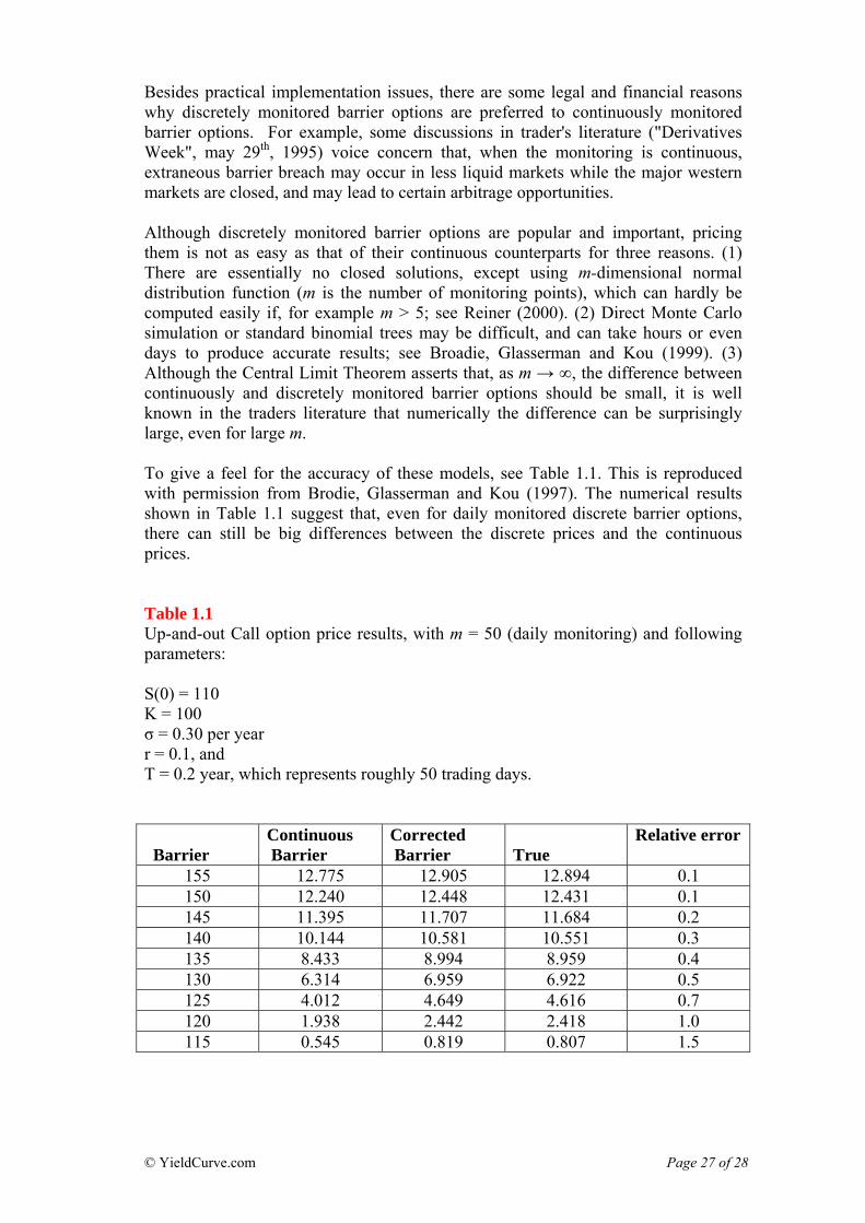
Besides practical implementation issues, there are some legal and financial reasons why discretely monitored barrier options are preferred to continuously monitored barrier options. For example, some discussions in trader's literature ("Derivatives Week", may 29th, 1995) voice concern that, when the monitoring is continuous, extraneous barrier breach may occur in less liquid markets while the major western markets are closed, and may lead to certain arbitrage opportunities. Although discretely monitored barrier options are popular and important, pricing them is not as easy as that of their continuous counterparts for three reasons. (1) There are essentially no closed solutions, except using m-dimensional normal distribution function (m is the number of monitoring points), which can hardly be computed easily if, for example m > 5; see Reiner (2000). (2) Direct Monte Carlo simulation or standard binomial trees may be difficult, and can take hours or even days to produce accurate results; see Broadie, Glasserman and Kou (1999). (3) Although the Central Limit Theorem asserts that, as m → ∞, the difference between continuously and discretely monitored barrier options should be small, it is well known in the traders literature that numerically the difference can be surprisingly large, even for large m. To give a feel for the accuracy of these models, see Table 1.1. This is reproduced with permission from Brodie, Glasserman and Kou (1997). The numerical results shown in Table 1.1 suggest that, even for daily monitored discrete barrier options, there can still be big differences between the discrete prices and the continuous prices. Table 1.1 Up-and-out Call option price results, with m = 50 (daily monitoring) and following parameters: S(0) = 110 K = 100 σ = 0.30 per year r = 0.1, and T = 0.2 year, which represents roughly 50 trading days. Barrier

Continuous Barrier

Corrected Barrier

True

Relative error

155 12.775 12.905 12.894 0.1 150 12.240 12.448 12.431 0.1 145 11.395 11.707 11.684 0.2 140 10.144 10.581 10.551 0.3 135 8.433 8.994 8.959 0.4 130 6.314 6.959 6.922 0.5 125 4.012 4.649 4.616 0.7 120 1.938 2.442 2.418 1.0 115 0.545 0.819 0.807 1.5


References Broadie, M., Glasserman, P. and Kou, S G. (1997), “A continuous correction for discrete barrier options”, Math. Finance 7, pp. 325-349 Broadie, M., Glasserman, P. and Kou, S G. (1999), “Connecting discrete and continuous path-dependant options”, Finan. Stochastics 3, pp. 55-82. Espen G. Haug., (1997), The complete guide to Option pricing, McGraw-Hill Heynen, R. C. and Kat, H. M. (1994b), “Partial barrier options”, Journal of Financial Engineering James, P., (2003), Option Theory, John Wiley & Sons Ltd M. S. Joshi,. (2003), The concepts and practice of mathematical finance, Cambridge University Press Kunitomo, N. and Ikeda, M. (1992), “Pricing options with curved boundaries”, Math. Finance Merton, R. C. (1973), “Theory of rational option pricing”, Bell J. Economic Management and Science 4, pp. 41-183. Merton, R. C., (1974) “On the pricing of corporate debt: the risk structure of interest rates”, Journal of Finance, 29 pp. 449-470 Reiner, E. (2000). Convolution Methods for Path-Dependant Options, Preprint, UBS Warburg Dillon Read Ritchken, P., (1995), “On pricing barrier options”, Journal of Derivatives 3, pp. 9-28 Rubinstien, M., Reiner, E., (1991), “Breaking down the barrier”, Risk 4, pp. 28-35 Wilmott, P., Howison, Dewynne, (1993), The Mathematics of Financial Derivatives, Cambridge University Press


exotic option: pricing path-dependent single barrier option

Documents