Exotic options and L�evy processesLaurent Nguyen-Ngoc Marc Yor

This version: Jan 20021 IntroductionA number of empirical studies have shown that the usual geometric Brownianmotion model used for the pricing of derivative securities is not appropriate inmany markets. As these products are becoming more and more popular, it is nolonger acceptable for a �nancial institution to use the geometric Brownian mo-tion regardless of its drawbacks. In the equities market, the smile phenomenonstands out amongst the main concerns: as European options have become liquidand can be treated as primary assets, it is important that a model matches theirprices if this is to be used to price (and hedge) exotic options. Several kinds ofalternative models have been and are still being developed, among which modelswith stochastic volatility (e.g. [37], [38]) or L�evy processes: Barndor�-Nielsen[5] introduced the NIG model, Madan and Seneta [20] proposed the VG model,extended in [32]. For an argument in favor of using L�evy processes in �nan-cial modelling, see [44]. Some models have also been investigated, which mixstochastic volatility and jumps ([9], [25], [29], [59]). Some of these models andtheir performance are reviews in other chapters of the present handbook [].Among exotic options, barrier and lookback options have the simplest struc-ture and were introduced a long time ago; they are today quite popular amonginvestors since they reduce the unwanted part of the risk carried by vanillaoptions. Not only traded on their own, they are commonly involved in moreelaborate structured products.In the framework of the geometric Brownian motion model, the problem hasbeen addressed and solved many times. Kunitomo and Ikeda [42] derive pricesfor barrier options with general boundaries (see also [3]); Geman-Yor [33] andSbuelz [58] use the Laplace transform method to price double barrier options;Pelsser [52] derives the same formulas using path integration.

Here, we deal with the pricing of barrier and lookback options when theunderlying asset price is modelled as eXt for a L�evy process X. By makinguse of purely probabilistic techniques, we obtain results that hold in the mostgeneral case, which embeds many popular models, such as the geometric Brow-nian motion (!), jump-di�usion, the Normal Inverse Gaussian model and theVariance-Gamma distribution.Thanks to the Pecherskii-Rogozin identity, we obtain a formula for the Laplace1

transform of option prices in terms of the Wiener-Hopf factors or the Laplaceexponent of the ladder process associated with X.This work is organized as follows. L�evy processes and their main mathemat-ical properties, as well as uctuation theory are introduced in Section 2. Wealso give some de�nitions and notations to be used in the sequel. In Section 3we review some uses of L�evy processes in �nance, before describing barrierand lookback options, and showing how their prices can be derived throughLaplace inversion. Pricing in particular cases is also studied, but the most gen-eral method gives some insight about hedging. Some examples are studied inSection 4, where some formulas {as explicit as possible{ are obtained for theLaplace transform of the option price. Section 5 concludes. Subsequently, anumerical example illustrates our technique in Appendix A, while Appendix Bpoints to possible extensions and future research.2 L�evy processesIn this section, we introduce L�evy processes and review their main mathematicalproperties. We put some emphasis on uctuation theory, as this is the leading"technology" which enables us to solve our valuation problem.2.1 De�nition and main propertiesIn this section, we de�ne L�evy processes and give a short review of their mainproperties. More details can be found in the books by Bertoin [11] and Sato[56] (see also [12], [57] for a short introduction) .We assume a probability space (;F ; P ) is given.De�nition 2.1 A real-valued process X = (Xt; t � 0) is called a L�evy processif it satis�es the following conditions

� for all s � 0, the shifted process (Xt+s � Xs; t � 0) is independent of(Xu; u � s);� for all 0 � s � t, the distribution of Xt�Xs coincides with the distributionof Xt�s;� X has a.s. right-continuous paths.

If X is a L�evy process, the distribution of X1 is in�nitely divisible because ofthe identityX1 = X1=n + (X2=n �X1=n) + � � �+ (X1 �X1�1=n)law= X(1)1=n +X(2)1=n + � � �+X(n)1=n

where the X(i)1=n are mutually independent variables, all distributed like X1=n.Conversely, to any in�nitely divisible distribution � on R one can associate a2

L�evy process X such that the law of X1 is �. In�nite divisibility of the lawof X1 is equivalent to the L�evy-Khintchine representation of its characteristicfunction: E[eiuX1 ] = e��(u)where �(u) = iau+ �22 u2 +ZR�f0g(1� eiux + iux1jxj<1)�(dx):(1)

In the above equation, a is a real number (the drift), � � 0 (the di�usioncoe�cient) and � is a �-�nite measure on R � f0g (the L�evy measure) whichsatis�es the condition Z (1 ^ x2)�(dx) <1(2)We then have for each t E[eiuXt ] = e�t�(u):(3)� is called the characteristic or L�evy exponent of X.The L�evy-Khintchine representation of the characteristic exponent � has acorresponding path interpretation: X can be decomposed as

Xt = at+ �Bt +Xs�t�Xs1j�Xsj>1 + lim�#0 Z(�)t(4)where� B is a standard Brownian motion,

� the sum makes sense because X has right-continuous paths hence �nitelymany jumps of absolute size > 1 in any �nite time interval,� for each � > 0, Z(�) is the martingale de�ned by

Z(�)t =Xs�t�Xs1�<j�Xsj�1 � t Z�<jxj�1 x�(dx);one can show that these martingales converge in L2, uniformly on anybounded time interval, as � goes to 0; the limit is a pure jump martingale.Note that the 3 processes above are mutually independent L�evy processes. Thedecomposition (4) is called the L�evy-Ito decomposition of the paths of X. Moredetails are given in [56, xx19-20].

From now on, we denote by (Ft; t � 0) the �ltration generated by X. Letus mention two well-known important properties of L�evy processes. The �rstone is the strong Markov property in the �ltration Ft. More precisely, for anyFt-�nite stopping time T , the shifted process (XT+t�XT ; t � 0) is independentof FT and has the same law as (Xt �X0; t � 0). The second one is that X isa special semimartingale (see [48, p. 310]). The semimartingale property canbe read from the L�evy-Ito decomposition; it is a special semimartingale becausethe compensator of the jumps is deterministic (cf. [39]).3

2.2 Fluctuation theoryWe now turn to a branch of the theory of L�evy processes, named uctuationtheory. Its aim is to study the joint behaviour of a process (here, our L�evyprocess) and its maximum. Fluctuations of random walks were �rst studied, forwhich Spitzer obtained many important results. Thanks to the independence ofincrements, most of these results can be transposed to L�evy processes. However,these results can be rediscovered by using excursion theory, an approach wefavor because it involves directly the paths of X. We follow closely Bertoin [11,Chap. VI] and Greenwood-Pitman [36]. For an account on uctuation theoryfor continuous time processes, see Bingham [13].Let Mt = sups�t Xs(5)the running maximum of the L�evy process X. The key point in the followingis that the re ected process M �X possesses the strong Markov property withrespect to the �ltration (Ft). Let L be a local time process at 0 of the re ectedprocess and denote by � its right-continuous inverse:

�t = inffu > 0; Lu > tg:(6)Put H(t) =M�(t) if �(t) <1; H(t) =1 otherwise:(7)The process (�;H) is called the ladder process, it is a two-dimensional L�evyprocess, each component being a subordinator. Roughly speaking, H is theprocess of the successive values of the supremum of X, when the intervals oftime where M is constant have been discarded; this is revealed by the use ofthe inverse local time as a time scale instead of the original calendar time.Let � be the Laplace exponent of the ladder process:

e�t�(�;�) = E[e���(t)��H(t)]:One of the main goals of uctuation theory is to compute the function �. Knowl-edge of this function will be needed in order to apply the main result of thissection, the Pecherskii-Rogozin identity (Theorem 2.1).We �rst proceed to give an expression of � in terms of the 1-dimensional distri-butions of X.

Let � be a random variable independent of X, exponentially distributedwith parameter q > 0 and denote G� = supft < � : Xt = Mtg. It is easyto see that M� = MG�� = XG��. Since the excursion process away from 0associated with M � X is a Poisson point process, we have that (Xt; t < G�)and (XG�+t � XG�� ; t � � � G�) are independent. In particular, the pairs ofvariables (G�;M�) and (��G�; X��M�) are independent. The following resultwill be used in section 4 for a number of models.

4

Proposition 2.1 There exists a constant k > 0 such that:�(�; �) = k exp�Z 1

0 dt Z 10 t�1(e�t � e��t��x)P (Xt 2 dx)�(8)

Proof . We have a decomposition of (�;X�) as the sum of two independent,in�nitely divisible random variables (G�;M�) and (��G�; X� �M�). Denotingby �, �+, �� the respective L�evy measures of these variables, we then have� = �+ + ��, with �+ (resp. ��) having support in [0;1) � [0;1) (resp.[0;1)�(�1; 0]). The L�evy measure of (�;X�) is given by t�1e�qtP (Xt 2 dx)dt(see [11, Lemma VI.7]) and can be decomposed ast�1e�qtP (Xt 2 dx)dt1x>0 + t�1e�qtP (Xt 2 dx)dt1x<0;

from which we conclude that �+ = t�1e�qtP (Xt 2 dx)dt1x>0.On the other hand, one can show using the theory of excursions, that the Laplacetransform of (G�;M�) is given byE[e��G���M� ] = �(q; 0)�(�+ q; �) :(9)

(this can be proved using a decomposition over excursion intervals as done inthe proof of Theorem 2.1 below). Putting pieces together, we have�(q; 0)�(�+ q; �) = exp��Z (1� e��t��x)�+(dt; dx)�

because there is no drift term in the distribution of (G�;M�). So�(�+ q; �) = �(q; 0) exp�Z 1

0 dtZ 10 P (Xt 2 dx)t�1e�qt(1� e��t��x)�

for all �; �; q > 0. Setting q = 1, we get the result for � > 1 and � > 0. Astandard argument of analytic continuation entails that the proposition is truefor all � > 0. �

Remark 2.1 The constant k = �(1; 0) is arbitrary as it depends only on thenormalization of the local time process L. Upon multiplying this process by somepositive constant, we can choose k = 1. However, we keep this kind of constantsin our general formulas; they will automatically (and consistently) be discardedin the pricing formulas.We now turn to prove the Pecherskii-Rogozin identity, which expresses the dou-ble Laplace transform of the joint distribution of hitting times and the valueof the process at such times in terms of the function �. This will be our maintool for pricing barrier and lookback options in a general setup. This identity

5

has been known for quite a long time and was �rst proved in [51] using Wiener-Hopf techniques of analysis. The proof we give here is based on the theory ofexcursions and avoids the original analytic arguments. See also [56, x49] for analternative proof.From now on, we suppose that 0 is regular for (0;1) relatively to X, i.e.infft > 0 : Xt > 0g = 0 a.s., and also that 0 is instantaneous for the re ectedprocess M �X, i.e. if infft > 0 : Mt �Xt 6= 0g = 0 a.s. If 0 is irregular, or isnot instantaneous, the set ft : Xt =Mtg is discrete, and elementary argumentsbased on the strong Markov property at the successive passage times at 0 of theprocess M �X su�ce to prove Theorem 2.1. For more details, see [11, Chap.IV].Theorem 2.1 (Pecherskii-Rogozin) For x > 0, de�ne T (x) = infft > 0 :Xt > xg the �rst passage time above x and K(x) = XT (x) � x the so-calledovershoot. For every �; �; q > 0, the following formula holds:Z 1

0 e�qxE[e��T (x)��K(x)]dx = �(�; q)� �(�; �)(q � �)�(�; q)(10)Before we prove the Pecherskii-Rogozin identity, we need the following re-sults:

Proposition 2.2 For x > 0, let �x := infft : H(t) > xg.1. The process Zx = H(�x)�x is a Markov process in the �ltration (F�x ; x >0).2. For all x > 0, it holds a.s. that T (x) = �(�x) and K(x) = Zx.

Remark 2.2 The identity in the above proposition is easy to understand fromthe intuitive interpretation of the process (�;H) given above. Indeed, the timeT (x) is an increase time point for M . The equality T (x) = �(�x) is just thechange of time-scale between M and H; the overshoot is expressed, in the newtime-scale, as K(x) =MT (x) � x = H�x � x:Proof .

1. This follows immediately from the general theory of time changes forMarkov processes.2. We �rst show that T (x) is in the range of � . Since T (x) is a zero ofM�Xit is enough to show that it is not the left end-point of an excursion interval{it will then be a right end-point. We will therefore have T (x) = �(l(x))and also l(x) = L(T (x)).Suppose on the contrary that T (x) is the left end-point of an excursioninterval (�(a�); �(a)) (so (T (x) = �(a�)). We then have M > X on an

6

open interval (T (x); �(a)). On the other hand, T (x) is a stopping timeand the strong Markov property yields(MT (x)+t �XT (x)+t; t � 0) d= (Mt �Xt; t � 0):

This is in contradiction with the fact that 0 is regular forM�X, relativelyto [0;1).Let us now show that l(x) = �x, which will end the proof. We distinguishbetween two cases:� H(l(x)) > x. Then H(l(x)) = M�(l(x)) = MT (x) = XT (x) > x. Onthe other hand, Xt � x for all t < T (x) = �(l(x)) and for t < l(x)we have �(t) < �(l(x)). If H(t) > x, then T (x) � �(t), which doesnot hold, so that H(t) � x for t < l(x), meaning that l(x) = �x.� H(l(x)) = x. As in the previous case, we have H(t) � x for t < l(x).On the other hand, the Markov property implies that X visits [0;1)immediately after T (x) a.s. So for t > l(x), we have H(t) =M�(t) >M�(l(x)) = x, i.e. l(x) = �x.

�

Lemma 2.1 For all u � 0, �M�(u) = �M�(u�) = uProof . We have:

�M�(u) = infft : H(t) > H(u)g = uand �M�(u�) = infft : H(t) > H(u�)g � ubecauseH is increasing. Also, we have �M�(u�) � �M�(u) so the proof is complete.�

Lemma 2.2 �x is continuous, and �H , the L�evy measure of H satis�esZ 10 �H(dx) = +1:

Proof . We have that H(s) < H(t) for any s < t; it follows that � is continuous.Now, the jump part of H is not a compound Poisson process because of thehypothesis that 0 is a regular point for (0;1) relatively to M �X. Hence itsL�evy measure cannot be �nite. �

Lemma 2.3 The following identity between measures holds a.s:dx1H(�x)=x = dHd�xwhere dH is the drift of the L�evy process H.

7

Proof . For a > 0, denote by l1(a) the size of the �rst jump of H which isgreater than a. Fix c > 0, then for a < c, since the jump part of H is a Poissonpoint process with intensity measure �H :P [l1(a) > c] = �H([c;1))�H([a;1)) ! 0; a! 0

so that 0 is a regular point for the process Z introduced in Proposition 2.2. Onthe other hand, for a > c,P [l1(c) > a] = �H([a;1))�H([c;1)) ! 0; a!1

so that 0 is also recurrent for Z. It is easily seen that the sets fx : Zx = 0g andfx : H(�x) = xg coincide, and that � increases only on the set fx;9t : H(t) =H(t�) = xg = fx : H(�x) = xg. So � is a local time process for Z (see [11,Chap. IV]). Hence, ([11, Prop. IV.6])Z x0 1(Zy=0)dy = dH�x

where dH is the drift of H. This concludes the proof. �

There is a more intuitive argument for the above result. Indeed, as a subordi-nator, H has the L�evy-Ito representationHt = dHt+ Z t

0Z h (�� �H)(ds; dh)

where �H is the L�evy measure of H and � is a random Poisson measure withintensity �H . It follows that � has locally a representation�x = 1dH x1x2Awhere A = fx : H(�x) = xg and is constant on the set corresponding to jumpsof H. We conclude that dHd�x = 1H(�x)=xdx.

Proof of Theorem 2.1. First we split the quantity of interest over theexcursion intervals of the process Z in the above lemma:Z 10 e�qxE[e��T (x)��K(x)]dx = I + II

where I := E �Z 10 e�qxe���(�x)��(H(�x)�x)1H(�x)>xdx�

and II := E �Z 10 e�qxe���(�x)��(H(�x)�x)1H(�x)=xdx� :

8

The �rst term I may be split over the excursion intervals according toI = E "Xu>0

Z H(u)H(u�) e�qx���(�(x))��(H(�x)�x)dx#

Let us perform the change of variables x = H(u)� (h�H(u�)), so thatI = E "Xu>0

Z H(u)H(u�) e�q[H(u)�h+H(u�)]���(�H(u)�h+H(u�))��[H(�H(u)�h+H(u�))�H(u)+h�H(u�)]dh#

= E "Xu>0Z H(u)H(u�) e(q��)(h�H(u�))���(u)�qH(u)dh#

since according to Lemma 2.1, we have �H(u) = �H(u�) = u = �H(u)�(h�H(u�))for all h 2 (H(u�); H(u)). SoI = E "Xu>0 e(q��)H(u�)���(u�)�qH(u�)��(�(u)��(u�))�q(H(u)�H(u�)) Z H(u)�H(u�)

0 e(q��)hdh#Let �(t; h) = e��t�qh and apply the compensation formula ([11, Chap. 0])toget

I = E "Z 10 du�(�(u); H(u))Z �(dt; dh)e�(�t+qh) Z h

0 e(q��)vdv#= 1(q � �)�(�; q)

Z �(dt; dh)e��t(e��h � e�qh)where �(dt; dh) is the L�evy measure of the bivariate L�evy process (�;H). TheL�evy-Khintchine representation for � reads

�(�; �) = d��+ dH� + Z (1� e��t��h)�(dt; dh)wherefrom we deduce thatZ �(dt; dh)e��t(e��h � e�qh) = �(�; q)� �(�; �) + (� � q)dHand we �nally obtain

I = �(�; q)� �(�; �)(q � �)�(�; q) � dH�(�; �) :(11)Let us now consider the second term. According to Lemma 2.3:

II = E �Z 10 e�qx���(�x)��(H(�x)�x)1H(�x)=xdx�

= E �Z 10 e�qx���(�x)dHd�x� :

9

Since � is continuous, we can perform the change of variables u = �x in theintegral; this yieldsII = dHE �Z 1

0 e�qH(u)���(u)du�= dH�(�; q) :(12)

Combination of Equations (11) and (12) entails the Pecherskii-Rogozin identity.�

Remark 2.3 When the process X has no positive jumps, we have XT (x) = xa.s. This case is considered in a simpler manner in the next section.Denote by X̂ the dual L�evy process of X, namely X̂t = �Xt and by �̂the Laplace exponent of the ladder process associated with X̂. According toProposition 2.1, we have�̂(�; �) = k̂ exp�Z 1

0 dtZ 10 t�1(e�t � e��t��x)P (�Xt 2 dx)�

= k̂ exp�Z 10 dtZ 0

�1 t�1(e�t � e��t��x)P (Xt 2 dx)� :In particular, we have

�(�; 0) = k exp�Z 10 t�1(e�t � e��t)P (Xt � 0)dt�

�̂(�; 0) = k̂ exp�Z 10 t�1(e�t � e��t)P (Xt � 0)dt�

so that�(�; 0)�̂(�; 0) = kk̂ exp�Z 1

0 t�1(e�t � e��t)dt�= kk̂�(13)

where the last equality follows from using the Frullani integral: a ln(1 + �=b) =R10 (1 � e��t)at�1e�btdt. On the other hand, it is an easy consequence of theindependence of M� and X� �M� that the following holds:qq + � = �+q ��q(14)where �+q (resp. ��q ) is the characteristic function of M� (resp. X� � M�).This identity is known as the Wiener-Hopf factorization. From equation (9) wededuce that �+q (u) = �(q; 0)�(q;�iu)(15+)

10

and using duality, we have similarly��q (u) = �̂(q; 0)�̂(q; iu) :(15�)

So combining equations (13), (14), (15+) and (15�), �̂ can be deduced from �by the formula �(q;�iu)�̂(q; iu) = kk̂(q + �(u)):(16)2.3 L�evy processes with no positive jumpsWe now turn to the case when the L�evy process X has no positive jumps (X isthen called spectrally negative); in this case, the support of the L�evy measureis contained in (�1; 0). Note that by considering the dual process, this studyapplies to the case when X has no negative jumps. The results we present herealready appear in e.g. [62], where they are obtained by a �ne analysis of theLaplace exponent ; we use quite di�erent techniques that rely on martingaletheory; see also [11].Since there are no positive jumps, we can consider the Laplace exponent ,de�ned by E[e�Xt ] = et (�); � > 0;(17) is well-de�ned because X has no positive jumps and the Laplace transform ofa Gaussian variable is �nite. This formula holds indeed for all complex � suchthat <(�) > 0.The equation (�) = 0 has at least one solution; denote the largest one by�(0). Then is a bijection when restricted to [�(0);1) and we denote by� the inverse bijection. Standard martingale arguments will yield the Laplacetransform of the �rst passage times T (x).Indeed, since (�) <1, it is clear that e�Xt�t (�) is a martingale; becauseT (x) is a stopping time, the optional sampling theorem gives

E[e�XT (x)�T (x) (�)1T (x)<1] = 1:(18)Now because X has no positive jumps, the equality XT (x) = x holds a.s. onfT (x) <1g, so that the preceding equation can be written

E[e�T (x) (�)1T (x)<1] = e��x(19)or, considering the inverse bijection:

E[e��T (x)1T (x)<1] = e�x�(�):(20)Note that the set fT (x) = 1g is not necessarily P -negligible: it has positiveprobability if and only if �(0) > 0, and then the law of T (x) has an atom at+1: P [T (x) = +1] = 1� e�x�(0).

In the case of no positive jumps, we have the following nice property of therunning maximum.11

Proposition 2.3 Let � be an exponential variable with parameter q, indepen-dent of X. Then M� has an exponential distribution with parameter �(q).Proof . For x > 0, we have the following chain of equalitiesP (M� � x) = P (Tx � �)

= Z 10 qe�qtP (Tx � t)dt

= E �Z 1Tx qe�qtdt� by Fubini's theorem

= E[e�qTx1(Tx<1)]= e�x�(q)as required. �

We end this section by the following remark. The absence of positive jumpsensures that the ladder height process is given by Ht =M�(t) = t for �(t) <1.The bivariate Laplace exponent � is now especially simple.Theorem 2.2 The bivariate Laplace exponent � of the ladder process is givenby �(�; �) = �(�) + �:(21)The bivariate Laplace exponent of the dual ladder process is given by�̂(�; �) = kk̂ �� (�)�(�)� � :(22)

Proof . Because X has no positive jumps, its supremum functional M iscontinuous and additive for M �X. Moreover it is easy to see that M increasesexactly on the set ft : Xt = Mtg. Therefore M can be used as a local time forthe re ected process M �X (see [11, Th. VII.1]). It follows immediately thatthe ladder height process is simply H(t) = t. The inverse local time is then seento coincide with the passage time process T (x), and we have shown above thatE[e��T (x)] = e�x�(�):It follows that �(�; �) = � +�(�). Now recall identity (16) to get�̂(�; �) = kk̂�+ �(�i�)�(�;��)

= kk̂ �� (�)�(�)� ��

Hence, to deal with the case when the L�evy process X has no negative jumps,we may simply consider that it is the dual process of a L�evy process X̂ with nopositive jumps.12

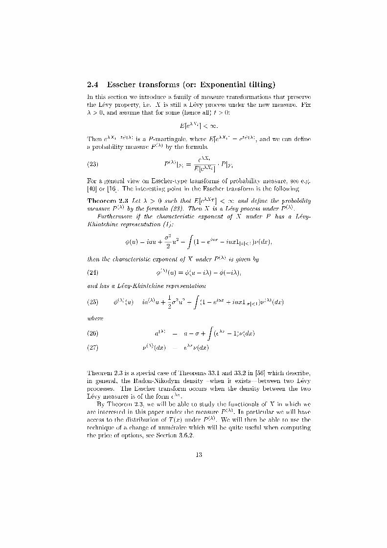
2.4 Esscher transforms (or: Exponential tilting)In this section we introduce a family of measure transformations that preservethe L�evy property, i.e. X is still a L�evy process under the new measure. Fix� > 0, and assume that for some (hence all) t > 0:E[e�Xt ] <1:

Then e�Xt�t (�) is a P -martingale, where E[e�Xt ] = et (�), and we can de�nea probability measure P (�) by the formulaP (�)jFt = e�XtE[e�Xt ] � P jFt(23)

For a general view on Esscher-type transforms of probability measure, see e.g.[40] or [16]. The interesting point in the Esscher transform is the followingTheorem 2.3 Let � > 0 such that E[e�XT ] < 1 and de�ne the probabilitymeasure P (�) by the formula (23). Then X is a L�evy process under P (�).Furthermore if the characteristic exponent of X under P has a L�evy-Khintchine representation (1):

�(u) = iau+ �22 u2 +Z (1� eiux � iux1jxj<1)�(dx);

then the characteristic exponent of X under P (�) is given by�(�)(u) = �(u� i�)� �(�i�);(24)

and has a L�evy-Khintchine representation�(�)(u) = ia(�)u+ 12�2u2 +

Z (1� eiux + iux1jxj<1)�(�)(dx)(25)where

a(�) = a+ � + Z (e�x � 1)�(dx)(26)�(�)(dx) = e�x�(dx)(27)

Theorem 2.3 is a special case of Theorems 33.1 and 33.2 in [56] which describe,in general, the Radon-Nikodym density {when it exists{ between two L�evyprocesses. The Esscher transform occurs when the density between the twoL�evy measures is of the form e�x.By Theorem 2.3, we will be able to study the functionals of X in which weare interested in this paper under the measure P (�). In particular we will haveaccess to the distribution of T (x) under P (�). We will then be able to use thetechnique of a change of num�eraire which will be quite useful when computingthe price of options, see Section 3.6.2.13

3 Pricing of Barrier and Lookback optionsIn this section, we present barrier and lookback options, and explain how The-orem 2.1 can be used to derive their price in a fairly general setting. We beginby introducing the framework in which this will be done.3.1 The modelWe consider a �nancial market the uncertainty of which is described by a prob-ability space (;F ; P ) and that consists of one riskless asset with a constant(risk-free) rate of return r and a risky asset whose price process St satis�esSt = S0eXt(28)where X is a L�evy process. Using the Esscher transform, the L�evy process X inEquation (28) can be considered under a locally equivalent measure such thate�rtSt is a martingale in its natural �ltration (Ft), which coincides with thenatural �ltration of X. We assume that P is used as a pricing measure and themarket contains no arbitrage opportunities, so that the price of a contingentclaim with maturity T is given by the expectation under P of its discountedpayo�.Such a model has been considered in [24], [15], [61] among others. Howevermost of this work is dedicated to abstract valuation of contingent claims andthe only example provided is that of vanilla options |except [15] who use ana-lytic techniques and whose results do not cover all cases. Special cases will bestudied in Section 4, and include well-known models such as the Normal InverseGaussian and the Variance Gamma distribution.3.2 Di�erence with Brownian / di�usion modelsBefore we turn to our main results, let us explain what changes dramaticallywhen L�evy processes are used in �nancial modelling. Until recently, processesused to model the price of an asset in view of the valuation of derivative in-struments were essentially di�usion processes, that is, processes solution to anSDE dSt = btdt+ �tdWt;(29)where W is a Brownian motion. The �rst such example is the most famousBlack-Scholes model [14], where bt = b and �t = � are constant over time.However, this model turned out to be unsatisfactory, because market observa-tions highly contradict the hypotheses. In particular, the volatility is not thesame for all strikes and maturities of vanilla options, contrary to what the modelpostulates. Extensions have been investigated, letting b and � be stochastic pro-cesses; the most famous ones are probably Dupire's model, where � is assumedto be a function of t and St, and bt = 0, and, otherwise, stochastic volatilitymodels, where � is taken to be the solution to another SDE

d�t = �tdt+ tdBt14

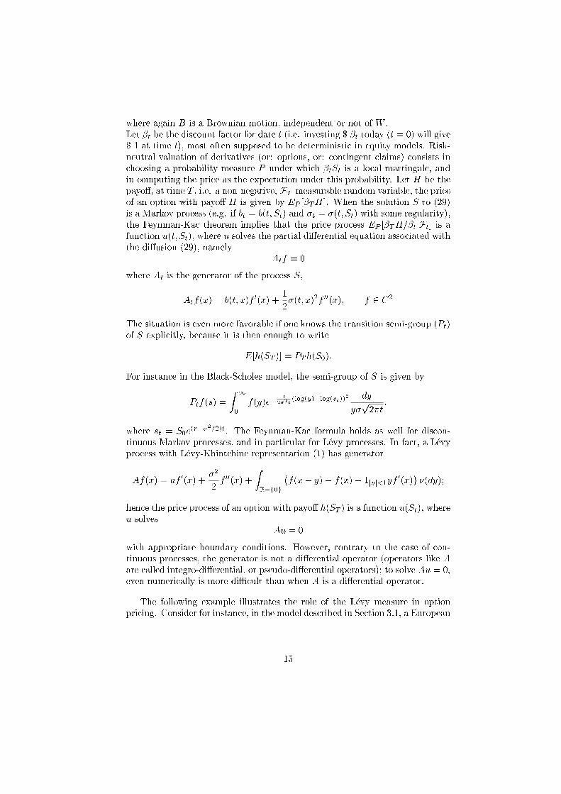
where again B is a Brownian motion, independent or not of W .Let �t be the discount factor for date t (i.e. investing $ �t today (t = 0) will give$ 1 at time t), most often supposed to be deterministic in equity models. Risk-neutral valuation of derivatives (or: options, or: contingent claims) consists inchoosing a probability measure P under which �tSt is a local martingale, andin computing the price as the expectation under this probability. Let H be thepayo�, at time T , i.e. a non-negative, FT -measurable random variable, the priceof an option with payo� H is given by EP [�TH]. When the solution S to (29)is a Markov process (e.g. if bt = b(t; St) and �t = �(t; St) with some regularity),the Feynman-Kac theorem implies that the price process EP [�TH=�tjFt] is afunction u(t; St), where u solves the partial di�erential equation associated withthe di�usion (29), namely Atf = 0where At is the generator of the process S,Atf(x) = b(t; x)f 0(x) + 12�(t; x)2f 00(x); f 2 C2

The situation is even more favorable if one knows the transition semi-group (Pt)of S explicitly, because it is then enough to writeE[h(ST )] = PTh(S0):

For instance in the Black-Scholes model, the semi-group of S is given byPtf(s) = Z 1

0 f(y)e� 12�2t (log(y)�log(st))2 dyy�p2�t :where st = S0e(r��2=2)t. The Feynman-Kac formula holds as well for discon-tinuous Markov processes, and in particular for L�evy processes. In fact, a L�evyprocess with L�evy-Khintchine representation (1) has generatorAf(x) = af 0(x) + �22 f 00(x) +

ZR�f0g �f(x+ y)� f(x)� 1jyj<1yf 0(x)� �(dy);

hence the price process of an option with payo� h(ST ) is a function u(St), whereu solves Au = 0with appropriate boundary conditions. However, contrary to the case of con-tinuous processes, the generator is not a di�erential operator (operators like Aare called integro-di�erential, or pseudo-di�erential operators); to solve Au = 0,even numerically is more di�cult than when A is a di�erential operator.The following example illustrates the role of the L�evy measure in optionpricing. Consider for instance, in the model described in Section 3.1, a European

15

call option, with payo� H = h(ST ) = (ST � K)+. Also assume there are nointerest rates, so that the price is given byE[(ST �K)+] = Z 1

K P (ST > x)dx= Z 1

K P (XT > ln(x=S0))dx= S0 Z 1

k P (XT > y)eydywhere k = ln(K=S0) and X is L�evy. Suppose for the sake of the argument thatX has no drift, no Brownian component and �nite L�evy measure �. Then, bythe compensation formula, we getP (XT > y) = 10>y + E Z T

0 ds ZR�f0g �(dx)(1Xs+x>y � 1Xs>y)= 1y<0 + Z T

0 dsE Z 0�1 �(dx)1x+y<Xs<y � Z T

0 dsE Z 10 �(dx)1y<Xs<y+x

= 1y<0 + Z T0 ds �E1Xs<y��(Xs � y)� E1Xs>y�+(Xs � y)�

where ��(z) = R z�1 �(dx) for z < 0 and �+(z) = R1z �(dx) for z > 0 are thetails of �. This shows the role played by the L�evy measure.Despite the di�culties underlined above, e�cient methods exist to price Eu-ropean options with L�evy processes. Since a L�evy processX is most often knownvia its L�evy exponent �, one can use Fourier inversion to compute P (XT > y);the following formula can be found in e.g. Lukacs [45]

P [XT > y] = 12 � 1�Z 10 e�iuye�T�(u) � eiuye�T�(�u)iu du:

Based on these and other considerations, several families of models havebeen developed that use L�evy processes and derive prices of vanilla options, andgeneral studies have also been made. A theoretical argument is developed in [44]that explains why L�evy processes could remedy some drawbacks of modellingwith continuous processes.Chan [24] examines European option pricing when the underlying price pro-cess is modelled as dSt = St�(btdt+ �tdYt)where Y is a L�evy process satisfying certain technical conditions, and b and �are deterministic functions. This model is more general than the one we willconsider, since S is then the exponential of a process with independent, but notstationary, increments (these processes are called additive processes in [56]). Asa choice of a pricing measure, Chan examines a generalized Esscher transform16

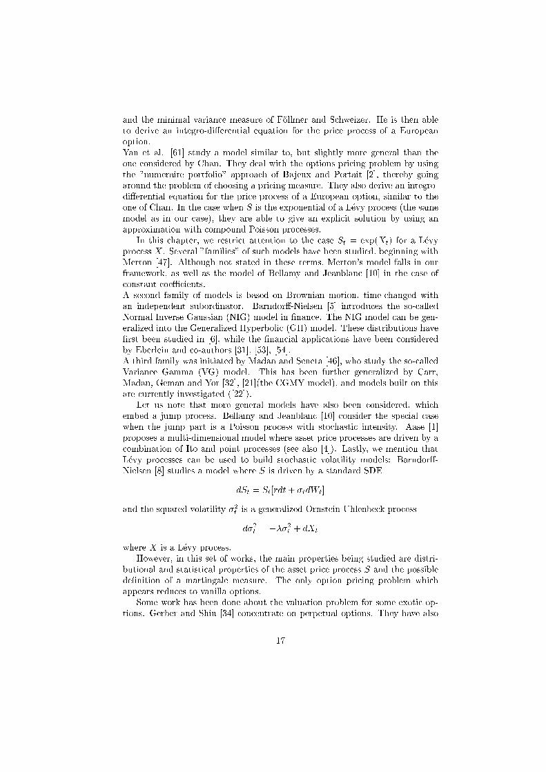
and the minimal variance measure of F�ollmer and Schweizer. He is then ableto derive an integro-di�erential equation for the price process of a Europeanoption.Yan et al. [61] study a model similar to, but slightly more general than theone considered by Chan. They deal with the options pricing problem by usingthe "numeraire portfolio" approach of Bajeux and Portait [2], thereby goingaround the problem of choosing a pricing measure. They also derive an integro-di�erential equation for the price process of a European option, similar to theone of Chan. In the case when S is the exponential of a L�evy process (the samemodel as in our case), they are able to give an explicit solution by using anapproximation with compound Poisson processes.In this chapter, we restrict attention to the case St = exp(Xt) for a L�evyprocess X. Several "families" of such models have been studied, beginning withMerton [47]. Although not stated in these terms, Merton's model falls in ourframework, as well as the model of Bellamy and Jeanblanc [10] in the case ofconstant coe�cients.A second family of models is based on Brownian motion, time-changed withan independent subordinator. Barndor�-Nielsen [5] introduces the so-calledNormal Inverse Gaussian (NIG) model in �nance. The NIG model can be gen-eralized into the Generalized Hyperbolic (GH) model. These distributions have�rst been studied in [6], while the �nancial applications have been consideredby Eberlein and co-authors [31], [53], [54].A third family was initiated by Madan and Seneta [46], who study the so-calledVariance Gamma (VG) model. This has been further generalized by Carr,Madan, Geman and Yor [32], [21](the CGMY model), and models built on thisare currently investigated ([22]).Let us note that more general models have also been considered, whichembed a jump process. Bellamy and Jeanblanc [10] consider the special casewhen the jump part is a Poisson process with stochastic intensity. Aase [1]proposes a multi-dimensional model where asset price processes are driven by acombination of Ito and point processes (see also [4]). Lastly, we mention thatL�evy processes can be used to build stochastic volatility models: Barndor�-Nielsen [8] studies a model where S is driven by a standard SDEdSt = St[rdt+ �tdWt]

and the squared volatility �2t is a generalized Ornstein-Uhlenbeck processd�2t = ���2t + dXt

where X is a L�evy process.However, in this set of works, the main properties being studied are distri-butional and statistical properties of the asset price process S and the possiblede�nition of a martingale measure. The only option pricing problem whichappears reduces to vanilla options.Some work has been done about the valuation problem for some exotic op-tions. Gerber and Shiu [34] concentrate on perpetual options. They have also17

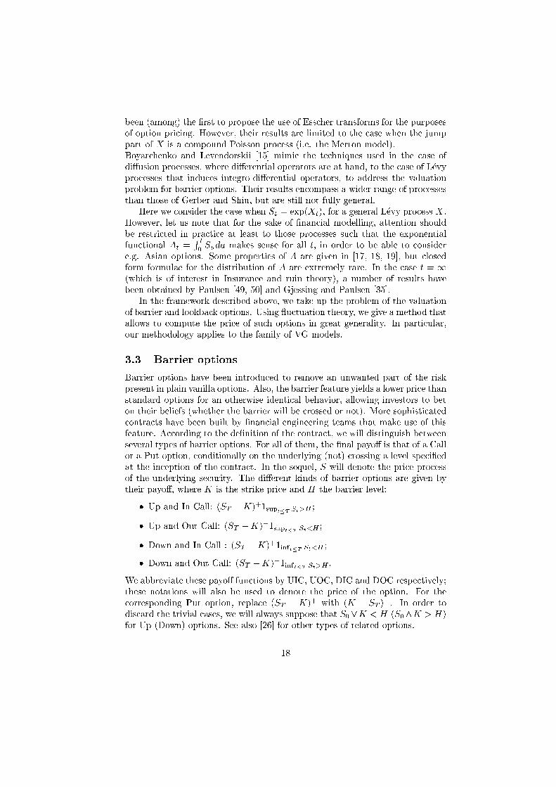
been (among) the �rst to propose the use of Esscher transforms for the purposesof option pricing. However, their results are limited to the case when the jumppart of X is a compound Poisson process (i.e. the Merton model).Boyarchenko and Levendorskii [15] mimic the techniques used in the case ofdi�usion processes, where di�erential operators are at hand, to the case of L�evyprocesses that induces integro-di�erential operators, to address the valuationproblem for barrier options. Their results encompass a wider range of processesthan those of Gerber and Shiu, but are still not fully general.Here we consider the case when St = exp(Xt), for a general L�evy process X.However, let us note that for the sake of �nancial modelling, attention shouldbe restricted in practice at least to those processes such that the exponentialfunctional At = R t0 Sudu makes sense for all t, in order to be able to considere.g. Asian options. Some properties of A are given in [17, 18, 19], but closedform formulae for the distribution of A are extremely rare. In the case t = 1(which is of interest in Insurance and ruin theory), a number of results havebeen obtained by Paulsen [49, 50] and Gjessing and Paulsen [35].In the framework described above, we take up the problem of the valuationof barrier and lookback options. Using uctuation theory, we give a method thatallows to compute the price of such options in great generality. In particular,our methodology applies to the family of VG models.3.3 Barrier optionsBarrier options have been introduced to remove an unwanted part of the riskpresent in plain vanilla options. Also, the barrier feature yields a lower price thanstandard options for an otherwise identical behavior, allowing investors to beton their beliefs (whether the barrier will be crossed or not). More sophisticatedcontracts have been built by �nancial engineering teams that make use of thisfeature. According to the de�nition of the contract, we will distinguish betweenseveral types of barrier options. For all of them, the �nal payo� is that of a Callor a Put option, conditionally on the underlying (not) crossing a level speci�edat the inception of the contract. In the sequel, S will denote the price processof the underlying security. The di�erent kinds of barrier options are given bytheir payo�, where K is the strike price and H the barrier level:

� Up and In Call: (ST �K)+1supt�T St>H ;� Up and Out Call: (ST �K)+1supt�T St<H ;� Down and In Call : (ST �K)+1inft�T St<H ;� Down and Out Call: (ST �K)+1inft�T St>H .We abbreviate these payo� functions by UIC, UOC, DIC and DOC respectively;these notations will also be used to denote the price of the option. For thecorresponding Put option, replace (ST � K)+ with (K � ST )+. In order todiscard the trivial cases, we will always suppose that S0_K < H (S0^K > H)for Up (Down) options. See also [26] for other types of related options.18

Before going further, let us point out the following relations between thepayo�s of barrier options and vanilla options:UIC(K;H) + UOC(K;H) = Call(K)DIC(K;H) +DOC(K;H) = Call(K)

which allow us to consider only the family of "In" options. Also, it is clearthat the pricing formula for "Down" options can be deduced from the pricingformula for "Up" options by considering the "dual" price process 1=S in placeof S. Lastly, because of the well known parity relation between Call and Putoptions, it is enough to deal with Call options. Hence we will give details onlyfor the "Up and In Call" option.Reduction to Binary optionsHaving restricted attention to the case of the Up and In Call option, we nowshow how to reduce the problem of pricing this option to that of pricing a Binary(or: Digital) option.The payo� of an Up and In barrier Call option is

(ST �K)+1supt�T St>H :(30)Di�erentiating this expression with respect to the strike price K, we obtain

�1ST>K1supt�T St>H :(31)which is the negative of the payo� of a Binary Up and In Call option with strikeprice K and barrier H (abbreviated as BinUIC(K,H)). By arbitrage, the samerelation must hold between the prices:Proposition 3.1 For all K and H

UIC(K;H) = Z 1K BinUIC(k;H)dk:(32)

Note that this relation does not depend on the model under consideration.Similar relations hold for other types of (barrier) options.3.4 Lookback optionsLookback options have been introduced to keep track of the minimum (or max-imum) level reached by the asset price during the time interval of interest. The�xed strike lookback options call and put, have payo�

(maxt�T St �K)+ and (K �mint�T St)+;(33)

19

denoted by LBCallfi(K) and LBPutfi(K); the oating strike lookback calland put have payo�(ST � �mint�T St)+ and (�maxt�T St � ST )+(34)

denoted by LBCallfl(�) and LBPutfl(�).Also of interest are the variable notional call and put options with respectivepayo�s (ST �mint�T St)+mint�T St and (maxt�T St � ST )+maxt�T St(35)however we will restrict interest on the �rst two types.

To compute the price of �xed strike lookback options, all we need to knowis the distribution of the supremum or in�mum functional. Let us consider thecase of the supremum, the case of the in�mum being completely analogous. Thedistribution of the supremum functional can be deduced from that of the �rstpassage times, since maxt�T St > x() TSx � T:The distribution of TSx is characterized by a special case of the Pecherskii-Rogozin identity, by setting � = 0 in Eq. (10):Z 1

0 e�qxE[exp(��TSS0ex)]dx = �(�; q)� �(�; 0)q�(�; q) :Inverting this Laplace transform is then enough to compute the price of the�xed strike lookback call.Alternatively, we can consider the following strategy for pricing the �xedstrike lookback call. We have

(maxt�T St �K)+ = Z maxt�T StK dk= Z 1

K 1maxt�T St>kdkThe integrand can be seen as the payo� of a binary Up and In call option withbarrier level k and strike price 0. The prices must also satisfy this relationship:Proposition 3.2 For all K, it holds that

LBCallfi(K) = Z 1K BinUIC(0; k)dk(36)

We shall now show that the oating strike lookback options can be expressedin terms of Binary barrier options. Consider for instance the oating strike20

lookback put option. It is clear that(�maxt�T St � ST )+ = Z �maxt�T StST dk

= Z 10 1ST�k��maxt�T Stdk

= Z 10 1ST�k1maxt�T St� k� dk

and by the absence of arbitrage, the prices must stand in the same relationship:Proposition 3.3 For all �, we have

LBPutfl(�) = Z 10 BinUIP (k; k� )dk(37)

Note that if S0 � k� , the barrier feature is meaningless, so that BinUIP (k; k� )= BinPut(k) where BinPut(k) is the price of a binary put option, that payso� 1ST�k. Hence,LBPutfl(�) = Z k=�

0 BinUIP (k; k� )dk +Z 1k=�BinPut(k)dk:

As we will see later in section 3.6, it is not the most e�cient way of pricing op-tions to write them as integrals of appropriate related digital options. However,this is a totally general method and gives some insight on a possible hedgingstrategy.3.5 Pricing of the BinUIC optionAll that we need now is to compute the price of the BinUIC option. For thispurpose we will use the Pecherskii-Rogozin identity (10).First, rewrite the payo� in terms of the running maximum. The digitalbarrier option with barrier level H and strike K pays at maturity T :

1ST>K1MST>H(38)where MSt = sups�t Ss. Denoting by M the process Mt = sups�tXs, k =log(K=S0) and h = log(H=S0), this payo� can be expressed in terms of theL�evy process X: 1XT>k1MT>h:(39)Writing � = infft;MSt > Hg = infft;Mt > hg = T (h) with the notation ofsection 2 the �rst exit time from the interval (�1; h] for the process X, we canalso write this payo� as 1XT>k1��T :(40)

21

Let us now compute the price:p = e�rTE[1XT>k1��T ]= e�rTE[E[1XT>k1��T jF�]]= E[e�r�1��TE[e�r(T��)1XT>kjF�]]On the event f� � Tg, the inner conditional expectation is the price of a BinaryCall option when the spot is S0eX� and the maturity is T � �. Because of theMarkov property of the process X, this is a function of (�;X�) which we willdenote by BinCall(�;X�). This type of options can be valued by invertingthe Fourier transform of the log of the asset price |in our case, the L�evyprocess X (see e.g. [37] or [23]). The method consists in decomposing thepayo� into appropriate pieces and then performing a change of num�eraire oneach piece so that the price of the options is expressed through di�erent measures(probabilities) of the exercise set of the option. See subsection 3.6.2 for a directapplication of this technique to the case of barrier options.The case of a European Digital Call option is especially simple, since the priceof such an option whith maturity t and strike ek is

pDert = E[1Xt>k] = 1� P [Xt � k]:(41)It is then immediate to obtain the price by inverting the characteristic functionof X: P [Xt � k] = 12 + 12�

Z 10 e�iuke�t�(u) � eiuke�t�(�u)iu du

In order to end the computation of the barrier option price, we need thejoint law of � and X�. This law is characterized by its Laplace transform givenin Theorem 2.1. Mathematically, we have just stated the well-known fact that adistribution is characterized by its Laplace transform. This Laplace transformcan be inverted numerically to retrieve the distribution function of (�;X�),which can in turn be used to compute the price of the digital barrier options;hence the integrals giving the price of barrier and lookback options can |atleast in principle| be computed numerically. However, due to the dimension ofthe problem, this method is likely not to be very e�cient from a computationalpoint of view, especially if naive algorithms are used. An alternative to thenumerical integration required to invert the Laplace transform would be to usean expansion with respect to some appropriately chosen functions.In the next section we study some special cases when the formulas found beforecan be simpli�ed |the numerics are then simpli�ed accordingly.Remark 3.1 A parallel can be made with the technique employed in [33] tocompute the price of barrier options in the Black-Scholes model. They computethe Laplace transform in time (i.e. with respect to the maturity) of the randomvariable of interest. This amounts to making the maturity an independent ex-ponential time. The same approach can be taken here |and has actually beenone of the steps taken to derive the preceding formulas. Let � be an exponen-tial variable with an exponential distribution with parameter q > 0. Excursion22

theory teaches us that the variables M� and X� �M� are independent and theirFourier transforms are the Wiener-Hopf factors. So the Laplace transform, withrespect to the maturity, of the price of a �xed strike lookback option is readilylinked to the Wiener-Hopf factor �+.3.6 Simpli�cations in special casesAs mentioned above, the pricing formulas can be simpli�ed in some cases, lead-ing to reduction of the dimension of the numerical problem. However, to expressthe prices of options as integrals of elementary payo�s (namely digitals) pro-vides some insight about the hedge of these options.We �rst study the case when the background L�evy process has no positivejumps, in which case the overshoot is 0 a.s. Then we show how to use the Ess-cher transform in order to reduce the numerical cost of computing the price ofa barrier option.3.6.1 The case with no positive jumpAs noted in section 2.3, the problem we study is greatly simpli�ed when X hasno positive jumps since standard martingale arguments can be used.Since X has no positive jumps, the barrier level h can only be crossed con-tinuously. Therefore if we still denote by � the �rst hitting time of the interval(h;1), we have necessarily X� = h. This simple fact allows for huge simpli�-cations.As noticed in Section 2, the Laplace transform of � is given by (Equation(20)): E[e���] = e�h�(�)where � is the inverse bijection of the Laplace exponent of X. The problemhas one dimension less than the general case, a signi�cant improvement from anumerical point of view.Let us turn to the concrete example of a �xed strike lookback option. Propo-sition 2.3 asserts that if � is an exponential variable with parameter q, indepen-dent from X, then M� has an exponential distribution with parameter �(q).Hence,

E[(eM� � ek)+] = Z 10 (em � ek)+�(q)e�m�(q)dm

= �(q)�Z 1k e�m(�(q)�1)dm� ek Z 1

k e�m�(q)dm�= �(q)�e�k(�(q)�1)�(q)� 1 � e�k(�(q)�1)�(q)

�= e�k(�(q)�1) 1�(q)� 1this formula being true for all q such that �(q) > 1, i.e. q > (1).Hence, the Laplace transform in the maturity of the price of a �xed strike

23

lookback call option is given by |we denote by k the log-moneyness, k =ln(K=S0):Z 10 e�qtLBCallfi(t;K)dt = S0 Z 1

0 e�(q+r)tE[(eMt � ek)+]dt= 1q + rE[(eM� � ek)+]

where � is an exponential variable with parameter q + r, and by the foregoing,this is equal to 1(q + r)(�(q + r)� 1)e�k(�(q+r)�1)So in this special case, we only have to invert a one-dimensional Laplace trans-form. We give in Appendix A some numerical results based on this technique.3.6.2 Change of num�eraireIn order to avoid the integration required to obtain the price of e.g. a Knock-in Up barrier option or a Lookback Put option from the price obtained forthe corresponding digital option, one can use a change of measure in order todecompose the expectation we wish to compute into two similar pieces. To dothis, we have to make an additional hypothesis on X; however this hypothesisis not really restrictive and is quite reasonable from a �nancial point of view.Suppose that E[eX1 ] < 1; this implies that X, which represents the log-arithm of the returns has moments of all orders, which is quite sensible froma �nancial point of view. This hypothesis allows us to consider the Esschertransform of P de�ned by

PX jFt = eXTE[eXT ] � P jFt ;(42)for all t > 0. By Theorem 2.3, X remains a L�evy process under PX , and itsL�evy exponent �X under PX is given by�X(u) = �(u� i)� �(�i)(43)Consider for instance the case of a Knock-in Up barrier call option and supposefor simplicity that S0 = 1 and r = 0. Its payo� is(eXT �K)1XT>k1T (h)�T :Hence the price is given by:E[(eXT �K)1XT>k1T (h)�T ] = E[eXT 1XT>k1T (h)�T ]�KP (XT > k; T (h) � T ):The last term is exactly the price of a digital knock-in option and can be com-puted as explained before. We can deal with the �rst term in the following way.Applying the Esscher transform mentioned above, it can be written asPX [XT > k; T (h) � T ]:

24

This can be interpreted as the price of digital option with respect to a di�erentpricing measure. Because X remains a L�evy process under PX , the same com-putations as before can be made, leading to a similar result, only with di�erentparameters.This method can be applied to reduce the computational cost of the nu-merical computation, since it gets rid of a numerical integration. We have putit here separately because it requires a supplementary hypothesis on the L�evyprocess X (still keeping a good generality). However the general method de-velopped above, by decomposing the payo� into elementary products (namelydigitals) provides some insight on the hedging which is lost in this more e�cientmethod.4 ExamplesIn this section we give a few examples where the function � can be computedin terms of known functions. They include

� the usual geometric Brownian motion;� a jump-di�usion model, which is a particular case of the model consideredby [10];� The case when X is a subordinator and particularly the Gamma process;� the case of a NIG model, introduced by [5] and also studied by [15];� the variance-gamma model introduced by [20], to which the method in[15] does not apply.

4.1 The usual geometric BMThe geometric BM falls into our class of models and therefore we can apply theresults developed before. A �rst approach could be to compute � from formula(8) (see Proposition 2.1) since when X is a brownian motion with drift �, wehave P (Xt 2 dx) = P (N(�t; t) 2 dx) = g�t;t(x)dx(1)where gm;s2 denotes the density of a Gaussian variable with mean m and vari-ance s2.Now since X has continuous paths, and a fortiori no positive jumps, the sim-pli�ed approach of section 3.6.1 can be used. Indeed, this amounts to applyingthe well-known re ection principle for brownian motion. Specializing equation(20), we recover the well-known formula for the hitting times of Brownian mo-tion with drift �: E[e��T (x)] = e�x(��+p�2+2�):The change of num�eraire technique in this setting is also well-known thanks tothe Cameron-Martin formula. In fact, S remains a geometric brownian motion25

under the new probability, with the only di�erence that its drift coe�cient ismodi�ed. Using this and the explicit knowledge of the semigroup and resolventoperators for the Brownian motion, [33] have obtained very explicit formulasfor the Laplace transform in time of the price of a barrier option; specializingtheir results to L = 0, a = +1 (with their notation):�(�) = E Z 1

0 e��u(Su �K)+1TSH�udu= e��bg1(eb)where

g1(eb) = 2� eb(�+1)�2 � (� + 1)2 � Keb��2 � �2�+ e��bK�+1���(�+ �)(�+ � + 1) ;

b = log(H=S0) and �2=2 = � + �2=2.4.2 Jump-di�usionHere we consider a special case of the model studied by [10]. Let the process Sbe given by the SDE

dSt = St� [�dt+ �dWt + �dNt](2)where W is a standard Brownian motion, N is a Poisson process with constantintensity � and � > �1. The drift � is chosen so that e�rtSt is a martingale:

� = r � �22 � ��It is well known that S is the Dol�eans-Dade exponential, multiplied by a driftterm:

St = S exp ��r � �22 � ��� t+ �Wt + ln(1 + �)Nt�= SeXt

where X is the L�evy processXt = �r � �22 � ��� t+ �Wt + ln(1 + �)Nt:(3)

Choose �rst � > 0, and according to Section 2.3, let be the Laplaceexponent of �X, E[e�uXt ] = et (u); we have (u) = ��r � �22 � ���u+ 12�2u2 � � �1� (1 + �)�u� :(4)

26

Let � be the inverse of ; according to Theorem 2.2, the ladder exponent � isgiven by �(�; �) = c�� (�)�(�)� � :(5)The Laplace transform of the pair (T (x); XT (x)) is then given byZ 1

0 e�qxE[e��T (x)��(XT (x)�x)]dx =1q � �

�1� (�� (�))(�(�)� q)(�(�)� �)(�� (q))�(6)

The price of a Up and In Call option with strike priceK, barrierH and maturityT is given byBinUIC(K;H; T ) = Z T

0Z 1h BinCall(Sey;K; T � t)dF (t; y)(7)

where h = ln(H=S0) and F is the joint distribution function of (T (x); XT (x)),that can be obtained from the above Laplace transform.If we choose � < 0, the results of section 3.6.1 apply. Alternatively if we tryto follow the steps of [33], we �nd that the resolvent operators are given byV��(x) = E �Z 1

0 e��u�(Xu)dujX0 = x�= 1�p�

Z dy�(y) 1Xn=0

1n!����2

�n e��xn� ~Kn+ 12 (zn(x; y))(8)with � = p2�2(� + �) + �2, zn(x; y) = p��2 (n ln(1 + �)� x� y), K� are theMacdonald functions and ~K�(x) = p2=�x�K�(x). The complexity of the ex-pression of the resolvent operators makes it impossible to carry on the pro-gramme worked out in [33].Remark 4.1 In the case of the Merton model, which generalizes the jump-di�usion model studied above, Kou and Wang [41] have obtained some resultsabout T (x) when

Xt = �t+ �Wt + NtXi=1 Yiand the Yi have density

p�1e��1y1y>0 + (1� p)�2e��2y1y<0for some 0 � p � 1, �1 > 0, �2 > 0.

27

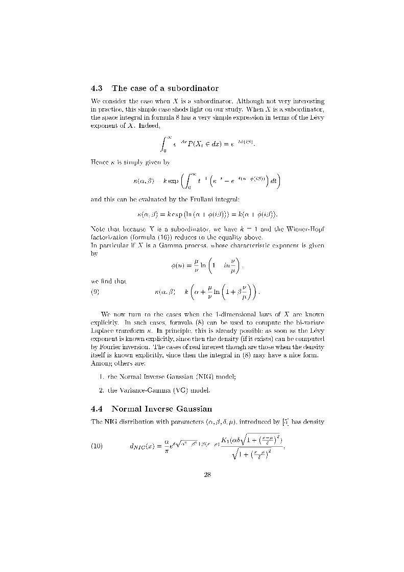
4.3 The case of a subordinatorWe consider the case when X is a subordinator. Although not very interestingin practice, this simple case sheds light on our study. When X is a subordinator,the space integral in formula 8 has a very simple expression in terms of the L�evyexponent of X. Indeed,Z 10 e��xP (Xt 2 dx) = e�t�(i�):

Hence � is simply given by�(�; �) = k exp�Z 1

0 t�1 �e�t � e�t(�+�(i�))� dt�and this can be evaluated by the Frullani integral:

�(�; �) = k exp (ln (�+ �(i�))) = k(�+ �(i�)):Note that because X is a subordinator, we have �̂ � 1 and the Wiener-Hopffactorization (formula (16)) reduces to the equality above.In particular if X is a Gamma process, whose characteristic exponent is givenby �(u) = �� ln

�1� iu��� ;

we �nd that �(�; �) = k��+ �� ln�1 + � ��

�� :(9)We now turn to the cases when the 1-dimensional laws of X are knownexplicitly. In such cases, formula (8) can be used to compute the bi-variateLaplace transform �. In principle, this is already possible as soon as the L�evyexponent is known explicitly, since then the density (if it exists) can be computedby Fourier inversion. The cases of real interest though are those when the densityitself is known explicitly, since then the integral in (8) may have a nice form.Among others are:1. the Normal Inverse Gaussian (NIG) model;2. the Variance-Gamma (VG) model.

4.4 Normal Inverse GaussianThe NIG distribution with parameters (�; �; �; �), introduced by [5] has densitydNIG(x) = �� e�p�2��2+�(x��)K1(��q1 + �x��� �2)q1 + �x��� �2 ;(10)

28

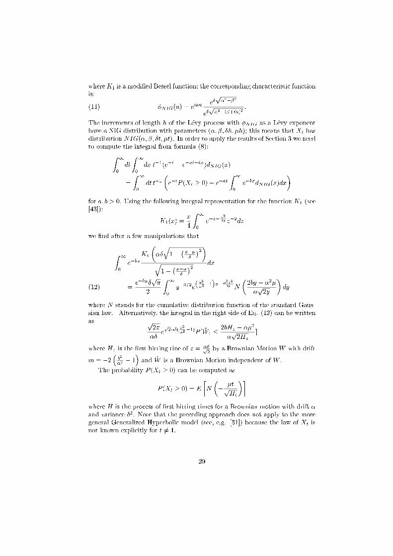
whereK1 is a modi�ed Bessel function; the corresponding characteristic functionis: �NIG(u) = ei�u e�p�2��2e�p�2�(�+iu)2 :(11)The increments of length h of the L�evy process with �NIG as a L�evy exponenthave a NIG distribution with parameters (�; �; �h; �h); this means that Xt hasdistribution NIG(�; �; �t; �t). In order to apply the results of Section 3 we needto compute the integral from formula (8):Z 1

0 dt Z 10 dx t�1(e�t � e�at�bx)dNIG(x)

= Z 10 dt t�1�e�tP (Xt � 0)� e�at Z 1

0 e�bxdNIG(x)dx�for a; b > 0. Using the following integral representation for the function K1 (see[43]): K1(x) = x4

Z 10 e�z� x24z z�2dz

we �nd after a few manipulations thatZ 10 e�bxK1���q1 + �x��� �2�q1 + �x��� �2 dx

= e�b��p�2Z 10 y�3=2e� b2�2�1�y��2�24y N �2by � �2��p2y

� dy(12)where N stands for the cumulative distribution function of the standard Gaus-sian law. Alternatively, the integral in the right side of Eq. (12) can be writtenas p2��� ep2��( b2�2�1)P [ ~W1 � 2bHz � ��2�p2Hz ]where Hz is the �rst hitting tine of z = ��p2 by a Brownian Motion W with driftm = �2� b2�2 � 1� and ~W is a Brownian Motion independent of W .The probability P (Xt � 0) can be computed as

P (Xt � 0) = E �N �� �tpHt��

where H is the process of �rst hitting times for a Brownian motion with drift �and variance �2. Note that the preceding approach does not apply to the moregeneral Generalized Hyperbolic model (see, e.g. [31]) because the law of Xt isnot known explicitly for t 6= 1.29

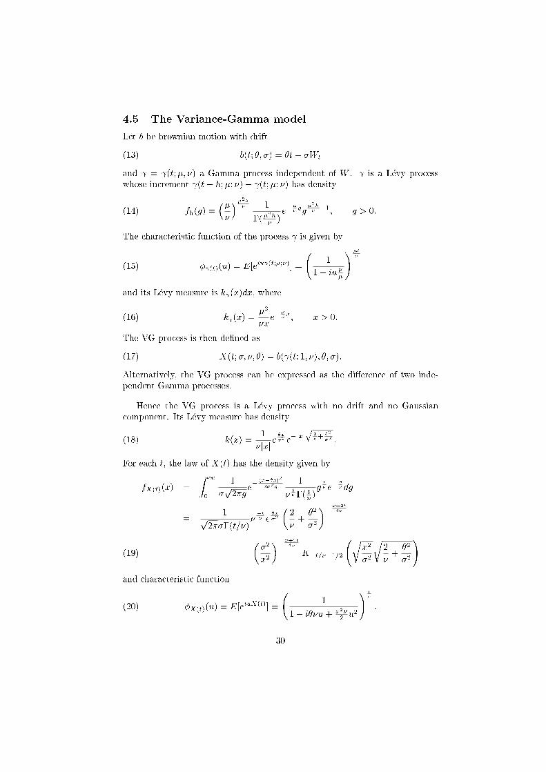
4.5 The Variance-Gamma modelLet b be brownian motion with driftb(t; �; �) = �t+ �Wt(13)

and = (t;�; �) a Gamma process independent of W . is a L�evy processwhose increment (t+ h;�; �)� (t;�; �) has densityfh(g) = ��� ��2h� 1�(�2h� )e��� gg �2h� �1; g > 0:(14)

The characteristic function of the process is given by� (t)(u) = E[eiu (t;�;�)] = 11� iu ��

!�t�(15)and its L�evy measure is k (x)dx, where

k (x) = �2�xe��� x; x > 0:(16)The VG process is then de�ned as

X(t;�; �; �) = b( (t; 1; �); �; �):(17)Alternatively, the VG process can be expressed as the di�erence of two inde-pendent Gamma processes.

Hence the VG process is a L�evy process with no drift and no Gaussiancomponent. Its L�evy measure has densityk(x) = 1�jxje �x�2 e�jxj

q 2�+ �2�2 :(18)For each t, the law of X(t) has the density given by

fX(t)(x) = Z 10 1�p2�g e� (x��g)22�2g 1� t� �( t� )g t� e� g� dg

= 1p2���(t=�)� �t� e �x�2�2� + �2�2

�� �+2t4���2x2

�� �+2t4� K�t=��1=2 rx2�2r2� + �2�2

!(19)and characteristic function

�X(t)(u) = E[eiuX(t)] = 11� i��u+ �2�2 u2! t� :(20)

30

In [46], [20], [23] the underlying stock is modelled as St = S0eXt where Xis a VG process. The general results we have derived apply to this situationand all we need now is to compute the bivariate Laplace exponent �(�; �). Byequation (8), this amounts to computing the integralZ 10 dtZ 1

0 1t (e�t � e��t��x)fX(t)(x)dx:Here again we can express P (Xt � 0) in terms of known functions. By usingFubini's theorem, it can be shown that

P (Xt � 0) = 12 + 1�(t=�)Z 10 e�x2=2 dxp2��ci

��2x2�2� ; t��

if � � 0, whileP (Xt � 0) = 1�(t=�)

Z 10 e�x2=2 dxp2��i

��2x2�2� ; t��

if � < 0, where �i is the incomplete Gamma function,�i(x; z) = Z x

0 e�uuz�1duand �ci is the complement �ci (x; z) = �(z)� �i(x; z).4.6 Stable processesStable processes are those L�evy processes which possess, just as the Brownianmotion, the scaling property : for some � 2]0; 2]

8k > 0; (Xkt; t � 0) (law)= (k1=�Xt; t � 0):(21)This property implies that P (Xt > 0) does not depend on t; the common value� is called the positivity parameter. Formula (2.7) then reduces to

�(�; �) = k exp�Z 10 dtt

��e�t � e��t Z 10 e��xP (Xt 2 dx)�� :

Unfortunately, except in the special cases of the Brownian motion and its hittingtimes, and the Cauchy process, the law P (Xt 2 dx) is not known explicitly,although a lot of information can be found in [30] and [63].However, some quantities related to the uctuation theory have simple ex-pression in the case of stable processes. It is shown in [55] thatP (X� 2 dy) = sin(��=2)� 1y

� xx� y��=2 dy; y > x(22)

for a symmetric stable process, where we recall � = infft : Xt > xg.31

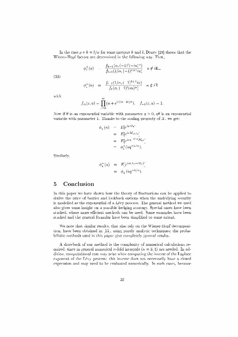
In the case �+ k = l=� for some integers k and l, Doney [28] shows that theWiener-Hopf factors are determined in the following way. First,�+1 (u) = fk�1(�; (�1)l(�iu)�)fl�1(1=�; (�1)k+1iu) u =2 iR�

(23)��1 (u) = fl�1(1=�; (�1)k+1iu)fk(�; (�1)l(iu)�) u =2 iR+

with fm("; u) = mYr=0(u+ ei"(m�2r)�); f�1("; u) = 1:

Now if � is an exponential variable with parameter q > 0, q� is an exponentialvariable with parameter 1. Thanks to the scaling property of X, we get:�+q (u) = E[eiuM� ]= E[eiuMq�=q ]= E[eiuq�1=�Mq� ]= �+1 (uq�1=�):

Similarly,��q (u) = E[eiu(X��M�)]= ��1 (uq�1=�):

5 ConclusionIn this paper we have shown how the theory of uctuations can be applied toderive the price of barrier and lookback options when the underlying securityis modelled as the exponential of a L�evy process. The general method we usedalso gives some insight on a possible hedging strategy. Special cases have beenstudied, where more e�cient methods can be used. Some examples have beenstudied and the general formulas have been simpli�ed to some extent.

We note that similar results, that also rely on the Wiener-Hopf decomposi-tion, have been obtained in [15], using purely analytic techniques; the proba-bilistic methods used in this paper give completely general results.A drawback of our method is the complexity of numerical calculations re-quired, since in general numerical n-fold integrals (n = 3; 4) are needed. In ad-dition, computational cost may arise when computing the inverse of the Laplaceexponent of the L�evy process: this inverse does not necessarily have a closedexpression and may need to be evaluated numerically. In such cases, because

32

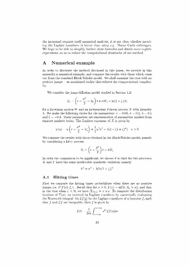
the integrand requires itself numerical analysis, it is not clear whether invert-ing the Laplace transform is better than using e.g. Monte Carlo techniques.We hope to be able to simplify further these formulas and obtain more explicitexpressions, so as to reduce the computational drawbacks of our method.A Numerical exampleIn order to illustrate the method discussed in this paper, we provide in thisappendix a numerical example, and compare the results with those which comeout from the standard Black-Scholes model. We shall examine the case with nopositive jumps |as mentioned earlier this reduces the computational complex-ity.

We consider the jump-di�usion model studied in Section 4.2:Xt = �r � �22 � ��� t+ �Wt + ln(1 + �)Nt

for a Brownian motion W and an independent Poisson process N with intensity�. We make the following choice for the parameters: r = 0:03, � = 0:2, � = 0:1and � = �0:3. These parameters are representative of parameters implied fromequities markets today. The Laplace exponent of X is given by (u) = u�r � �22 � ���+ 12u2�2 � �(1� (1 + �)u) u > 0

We compare the results with those obtained in the Black-Scholes model, namelyby considering a L�evy processYt = �r � ~�22

� t+ ~� ~WtIn order the comparison to be signi�cant, we choose ~� so that the two processesX and Y have the same predictable quadratic variation; namely

~�2 = �2 + �(ln(1 + �))2A.1 Hitting timesFirst we compute the hitting times probabilities when there are no positivejumps, i.e. P [T (x) � t]. Recall that for x > 0, T (x) = infft;Xt > xg, and thatin the case when � < 0, we have XT (x) = x a.s. To compute the distributionfunction of T (x), we inverted its Laplace transform by numerically evaluatingthe Bromwich integral: let Lf(q) be the Laplace transform of a function f , suchthat f and Lf are integrable, then f is given by

f(t) = 12i�Z +i1 �i1 etsLf(s)ds33

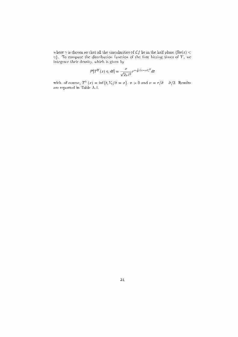
where is chosen so that all the singularities of Lf lie in the half plane fRe(z) < g. To compute the distribution function of the �rst hitting times of Y , weintegrate their density, which is given byP [TY (x) 2 dt] = xp2�t3 e� 12t (x��t)2dt

with, of course, TY (x) = infft; Yt=~� = xg, x > 0 and � = r=~� � ~�=2. Resultsare reported in Table A.1.

34

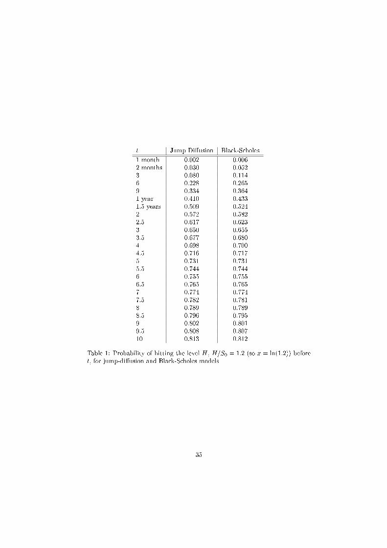
t Jump Di�usion Black-Scholes1 month 0.002 0.0062 months 0.030 0.0523 0.080 0.1146 0.228 0.2659 0.334 0.3641 year 0.410 0.4331.5 years 0.509 0.5242 0.572 0.5822.5 0.617 0.6233 0.650 0.6553.5 0.677 0.6804 0.698 0.7004.5 0.716 0.7175 0.731 0.7315.5 0.744 0.7446 0.755 0.7556.5 0.765 0.7657 0.774 0.7747.5 0.782 0.7818 0.789 0.7898.5 0.796 0.7959 0.802 0.8019.5 0.808 0.80710 0.813 0.812Table 1: Probability of hitting the level H, H=S0 = 1:2 (so x = ln(1:2)) beforet, for jump-di�usion and Black-Scholes models

35

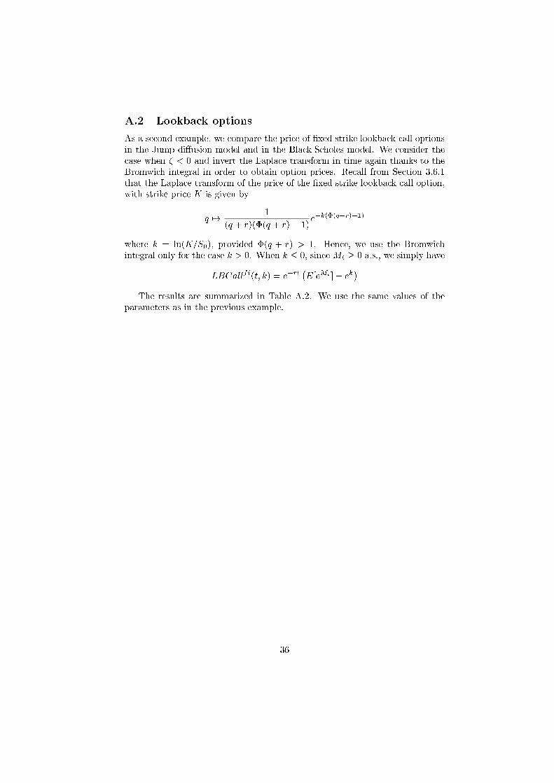
A.2 Lookback optionsAs a second example, we compare the price of �xed strike lookback call optionsin the Jump-di�usion model and in the Black-Scholes model. We consider thecase when � < 0 and invert the Laplace transform in time again thanks to theBromwich integral in order to obtain option prices. Recall from Section 3.6.1that the Laplace transform of the price of the �xed strike lookback call option,with strike price K is given byq 7! 1(q + r)(�(q + r)� 1)e�k(�(q+r)�1)

where k = ln(K=S0), provided �(q + r) > 1. Hence, we use the Bromwichintegral only for the case k > 0. When k � 0, since Mt � 0 a.s., we simply haveLBCallfi(t; k) = e�rt �E[eMt ]� ek�

The results are summarized in Table A.2. We use the same values of theparameters as in the previous example.

36

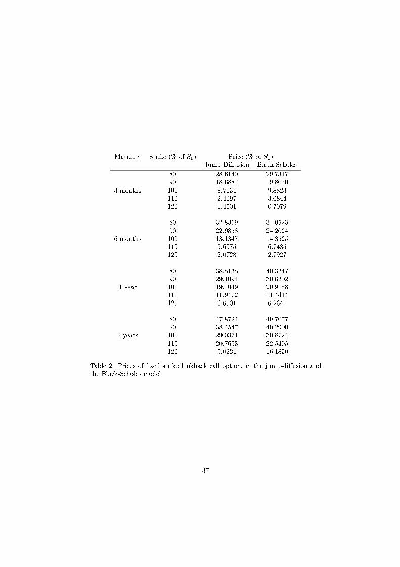
Maturity Strike (% of S0) Price (% of S0)Jump Di�usion Black-Scholes80 28.6140 29.731790 18.6887 19.80703 months 100 8.7634 9.8823110 2.4097 3.0844120 0.4501 0.707980 32.8369 34.052390 22.9858 24.20246 months 100 13.1347 14.3525110 5.6975 6.7485120 2.0728 2.792780 38.8138 40.324790 29.1094 30.62021 year 100 19.4049 20.9158110 11.9472 11.4414120 6.6501 6.264180 47.8724 49.707790 38.4547 40.29002 years 100 29.0371 30.8724110 20.7653 22.5405120 9.0224 16.1850

Table 2: Prices of �xed strike lookback call option, in the jump-di�usion andthe Black-Scholes model

37

B ExtensionsWe have established the Wiener-Hopf factorization for L�evy processes. However,it appears from empirical works that L�evy processes may not be suitable for themodeling of �nancial data series. In particular, the implied volatility surfacefrom L�evy processes is not consistent with those which are observed for manystocks and indices.Hence, in order to give our technique a wider range of applicability, it wouldbe desirable to extend it to other processes, in particular:

1. additive processes, i.e. processes with independent, but not stationary,increments;2. L�evy processes, time-changed with an independent increasing process.

The second case is in some sense a particular instance of the �rst one, since byconditioning on the time-change process, we �nd ourselves left with a processthat has independent, but not necessarily stationary, increments.B.1 Extension to additive processesIn the �rst case, the di�culty comes from the fact that the processes we dealwith are not homogeneous in time. However, some work can be done, but theresults we get are far less explicit than in the case of L�evy processes. We onlyoutline them here.Speci�cally, let X be an additive process. Thus, X is a non-homogeneousMarkov process. De�ne as before the re ected process ~Mt = Mt � Xt, whereMt = sups�tXs. Then, it is easy to see, thanks to the independence of theincrements of X, that ~M enjoys the simple Markov property (in the �ltration ofX). But ~M is not homogeneous, and does not enjoy the strong Markov propertyin the �ltration of X. Hence excursion theory cannot be applied directly.However, as is well-known, the time-space process Zt = (t; ~Mt) is a homoge-neous Markov process. In fact, as we end up working jointly in time and spacealready in the case of a L�evy process, it is reasonable to think that we will beable to derive some results also in the present case, by working directly on thetime-space process. However, all the properties will have to be \translated" ina convenient manner.We �rst note that the semi-group of (t; ~Mt) is a Feller semi-group (this canbe shown in much the same way as [11, Prop. VI.1]), so that Z possesses thestrong Markov property1.

Next, consider the set J = R+�f0g. This is a closed set, with empty interiorin R+�R+, the state space of the time-space process. We make the hypothesis1This can be stated another way: ~M enjoys a kind of \non-homogeneous strong Markov

property". Retaining the notations in [27], E�a [f � �T ] = F (T;XT ) for any �nite stopping

time T , any starting measure �, any time starting point a, and any bounded F1 measurablef , where F (t; x) = Ex

a+t[f ]

38

that every point in J is regular for J , namely8x = (t; 0) 2 J Px[inffu > 0; Zu 2 Jg = 0] = 1:(24)

In other words, for all t � 0, P [ ~Mt = 0 and inffu > t : ~Mu = 0g = 0] = 1. Thiscorresponds to the assumption that 0 is regular for itself in the L�evy case. Wealso assume that Px[inffu > 0; ~Mu > 0g = 0] = 1(25)for any x 2 J , which corresponds to the fact that 0 is an instantaneous pointin the homogeneous case. Note that according to Blumenthal's 0-1 law, each ofthe probabilities in (24) or (25) is either 0 or 1. If (24) or (25) is not satis�ed,the sucessive times at which Z returns in J form a discrete sequence Tn; thiscase will be examined separately.Hence, according to [27, Chap. XV, p.273], it is possible to de�ne a localtime process for J , i.e. an increasing continuous additive functional L of Z,such that the support of the measure dL is exactly J . We now want to studythe process Z in the local time scale.The inverse local time �t := inffu > 0; Lu > tg is a process with independentincrements, because of the additivity of L. However, � does not have stationaryincrements. We can de�ne the ladder height process H = S � � = X � � , andshow, just like in [11], that the bivariate process (�;H) is additive. It followsthat there exists a family of functions �u such thatE[e���u��Hu ] = e��u(�;�);

and each function �u has a L�evy-Khintchine representation�u(�; �) = �� (u)�+ �H(u)� + Z(0;1)�(0;1)(1� e��t��h)�lu(dt; dh):(26)

We can then follow the same lines as we did for L�evy processes in the proof ofthe Pecherskii-Rogozin identity 2.1. Lemmas 2.1 to 2.3 remain true; however,the formula in Lemma 2.3 must be amended asdx1H(�x)=x�H(�x)d�x:This is already a clue that formulas will not be as nice as for L�evy processes.In fact, by following exactly the same lines as in the proof of Theorem 2.1, weobtain:Z 1

0 dx e�qxE[e��T (x)��K(x)] = Z 10 du e��u(�;q)��u(�; q)� �u(�; �)q � �

�(27)where we recall T (x) denotes the �rst hitting times of X and K is the overshootat x: K(x) = XT (x) � x. This formula is in principle the same as formula (10);however, we do not know at the present time a formula similar to (8) that wouldenable us to actually compute the functions �u.

39

B.1.1 The case of irregular or holding pointsHere we enter the world of inhomogeneous Poisson processes.Let us �rst suppose that inffu > 0 : ~Mu = 0g > 0, Px-a.s. for some x 2 J .Then the Markov property entails that this holds for any x 2 J . It follows thatthe set of times at which ~M visits J is discrete.Suppose now that when it visits J , ~M is \held" there for some time �. Then� has an exponential distribution {whose parameter depends on the time when~M arrived in J .

B.2 Time changes of L�evy processesIn this paragraph, we deal with what we name time changes of L�evy processes,that is, models of the sort St = SeXt where the process X is taken to beXt = YCt , where Y is a L�evy process and C is an increasing process, independentof Y . Such models are discussed in e.g. [22].The results of the previous paragraph could be applied to the present case,since conditionnally on (Ct; t � 0), X is an additive process. However, under aslight assumption on C, we are able to get far more explicit and useful results.Assume that almost every path of C is continuous and strictly increasing.Then T (x) = CTY (x) as is easily seen, and as a consequenceE[h(T (x); XT (x))] = E[h(C(TY (x)); YTY (x))](28)

for any measurable and bounded function h. Hence, since we know the jointdistribution of (TY (x); YTY (x)), we also know the joint law of (T (x); XT (x)), andour results extends straightforwardly to the present case.This method allows to treat the model of [22], where Y is a CGMY (oranother L�evy) process, and C is the integrated square-root process:Ct = Z t

0 vsds;dvs = �(� � vs)ds+ �pvsdWswith W a Brownian motion, independent of Y .However, unfortunately, this does not extend to subordination (i.e. caseswhere C is a subordinator), since there is no continuous subordinator.

40

References[1] K. Aase. Contingent claim valuation when the security price is a combi-nation of an Ito process and a random point process. Stochastic processesand their applications, pages 185{220, 1988.[2] I. Bajeux and R. Portait. The numeraire portfolio: a new perspective on�nancial theory. European Journal of Finance, 3:291{309, 1997.[3] P. Baldi, L. Caramellino, and M.-G. Iovino. Pricing general barrier options:a numerical approach using sharp large deviations. Math. Finance, 9, 1999.[4] I. Bardhan and X. Chao. Pricing options on securities with discontinuousreturns. Stochastic processes and their applications, 48:123{137, 1993.[5] O. Barndor�-Nielsen. Processes of the normal inverse gaussian type. Fi-nance and stochastics, 2:41{68, 1998.[6] O. Barndor�-Nielsen and C. Halgreen. In�nite divisibility of the hyperbolicand generalized inverse Gaussian distributions. Zeitschrift f�ur Wahrschein-lichkeitstheorie und verwandte Gebiete, 1977.[7] O. Barndor�-Nielsen, T. Mikosch, and S. Resnick, editors. L�evy processesand applications. Birkhauser, 2001.[8] O. Barndor�-Nielsen and N. Shephard. Modelling by L�evy processes for�nancial econometrics, pages 283{318. In Barndor�-Nielsen et al. [7], 2001.[9] D. Bates. Jumps and stochastic volatility: exchange rate processes implicitin Deutsche mark options. Review of �nancial studies, 9:69{107, 1996.[10] N. Bellamy and M. Jeanblanc. Incompleteness of markets driven by a mixeddi�usion. Finance and Stochastics, 4(2):209{222, 2000.[11] J. Bertoin. L�evy processes. Cambridge University Press, 1996.[12] J. Bertoin. Some elements on L�evy processes. In Shanbhag and Rao [60],2000.[13] N. Bingham. Fluctuation theory in continuous time. Advances in AppliedProbability, 7:705{766, 1975.[14] F. Black and M. Scholes. The pricing of options and corporate liabilities.Journal of Political Economy, 81, 1973.[15] S. Boyarchenko and S. Levendorskii. European barrier options and Ameri-can digitals under L�evy processes. Technical report, University of Pennsyl-vania, dept. of Economics, 2000. Presented at the 1st Bachelier conference.[16] H. B�uhlmann, F. Delbaen, P. Embrechts, and A. Shiryaev. No-arbitrage,change of measure and conditional Esscher transforms. CWI Quarterly,9:291{317, 1997.

41

[17] P. Carmona, F. Petit, and M. Yor. Sur les fonctionnelles exponentielles decertains processus de L�evy. Stochastics and stochastic reports, 47:71{101,1994.[18] P. Carmona, F. Petit, and M. Yor. On the distribution and asymptoticresults for exponential functionals of L�evy processes. In M. Yor, editor,Exponential functionals and principal values related to Brownian Motion.Biblioteca de la Revista Matematica Iberoamericana, 1997.[19] P. Carmona, F. Petit, and M. Yor. Exponential functionals of L�evy pro-cesses, pages 41{55. In Barndor�-Nielsen et al. [7], 2001.[20] P. Carr, E. Chang, and D. Madan. The variance-gamma process and optionpricing. European Finance Review, 2:79{105, 1998.[21] P. Carr, H. Geman, D. Madan, and M. Yor. The �ne structure of assetreturns: an empirical investigation. Journal of Business, to appear, 2001.[22] P. Carr, H. Geman, D. Madan, and M. Yor. Stochastic volatility for L�evyprocesses. Econometrica, Submitted, 2001.[23] P. Carr and D. Madan. Option valuation using the fast Fourier transform.Journal of Computational Finance, 2, 1999.[24] T. Chan. Pricing contingent claims on stocks driven by L�evy processes.Annals of Applied Probability, 9(2):504{528, 1999.[25] M. Chernov, A.R. Gallant, E. Ghysels, and G. Tauchen. A new class ofstochastic volatility models with jumps: theory and estimation. Technicalreport, CIRANO, 1999.[26] M. Chesney, H. Geman, M. Jeanblanc, and M. Yor. Some combinations ofasian, parisian and barrier options. In M. Dempster and S. Pliska, editors,Mathematics of Derivative Securities, pages 61{87. Cambridge UniversityPress, 1997.[27] C. Dellacherie and P.A. Meyer. Probabilit�e et potentiel, vol. 4 Potentielassoci�e �a une r�esolvante. Processus de Markov. Hermann.[28] R. Doney. On Wiener-Hopf factorisation and the distribution of extremafor certain stable processes. Annals of Probability, 15:1352{1362, 1987.[29] D. Du�e, J. Pan, and K. Singleton. Transform analysis and asset pricingfor a�ne jump di�usions. Econometrica, 68:1343{1376, 2000.[30] E.B. Dynkin. Some limit theorems for sums of independent random vari-ables with in�nite mathemtatical expectation. Selected translations inMath. Stat. and Proba., 1:171{189, 1961.[31] E. Eberlein. Applications of generalized hyperbolic L�evy motions to �nance,pages 319{336. In Barndor�-Nielsen et al. [7], 2001.

42

[32] H. Geman, D. Madan, and M. Yor. Time changes for L�evy processes. Math.Finance, 2000.[33] H. Geman and M. Yor. Pricing and hedging double barrier options: aprobabilistic approach. Mathematical �nance, 6:365{378, 1996.[34] H. Gerber and E. Shiu. Martingale approach to pricing perpetual Americanoptions. ASTIN Bulletin, 24(195-220), 1994.[35] H. Gjessing and J. Paulsen. Present value distributions with applicationsto ruin theory and stochastic equations. Stochastic processes and theirapplications, 71:123{144, 1997.[36] P. Greenwood and J. Pitman. Fluctuation identities for L�evy processesand splitting at the maximum. Advances in Applied Probability, 12:893{902, 1980.[37] S. Heston. A closed-form solution for options with stochastic volatility withapplications to bond and currency options. Review of �nancial studies,6:327{343, 1993.[38] J. Hull and A. White. The pricing of options on assets with stochasticvolatility. Journal of Finance, 42:281{300, 1987.[39] J. Jacod and A. Shiryaev. Limit theorems fot stochastic processes. Springer,1987.[40] J. Kallsen and A. Shiryaev. The cumulant process and Esscher's change ofmeasure. Technical report, Universitat Freiburg, 2000.[41] S. Kou and H. Wang. First passage times of a jump di�usion process.Technical report, Columbia university, 2001.[42] N. Kunitomo and M. Ikeda. Pricing options with curved boundaries. Math.Finance, 2, 1992.[43] N. N. Lebedev. Special Functions and their Applications. Dover, 1972.[44] B. Leblanc and M. Yor. L�evy processes in �nance: a remedy to the non-stationarity of continuous martingales. Finance and Stochastics, 2:399{408,1998.[45] E. Lukacs. Characteristic functions. Gri�n statistical monographs andcourses, 1960.[46] D. Madan and E. Seneta. The Variance Gamma model for share marketreturns. Journal of Business, 63:511{524, 1990.[47] R. Merton. Option pricing when underlying stock returns are discontinuous.Journal of Financial Economics, 3:124{144, 1976.

43

[48] P.-A. Meyer. Un cours sur les int�egrales stochastiques. In S�eminaire deprobabilit�es X, Lecture notes in Mathematics, pages 245{400. Springer-Verlag, 1976.[49] J. Paulsen. Risk theory in a stochastic economic environment. Stochaticprocesses and their applications, 46:327{361, 1993.[50] J. Paulsen. Sharp conditions for certain ruin in a risk process with stochas-tic return on investments. Stochastic processes and their applications,75:135{148, 1998.[51] E. A. Pecherskii and B. A. Rogozin. On joint distributions of random vari-ables associated with uctuations of a process with independent increments.Theory of Probability and its Applications, 14:410{423, 1969.[52] A. Pelsser. Pricing double barrier options using Laplace transforms. Fi-nance and Stochastics, 4:95{104, 2000.[53] K. Prause. The generalized hyperbolic model: estimation, �nancial deriva-tives, and risk measures. PhD thesis, A. Ludwigs universitat Freiburg,1999.[54] S. Raible. L�evy processes in �nance: theory, numerics, and empirical facts.PhD thesis, A. Ludwigs universitat Freiburg, 2000.[55] D. Ray. Stable processes with absorbing barriers. Transactions of theAmerican Mathematical Society, 89:16{24, 1958.[56] K. Sato. L�evy processes and in�nitely divisible distributions. Cambridgestudies in advanced mathematics. Cambridge University Press, 1999.[57] Ken-Iti Sato. Basic results on L�evy processes, pages 3{37. In Barndor�-Nielsen et al. [7], 2001.[58] A. Sbuelz. A general treatment of barrier options. Technical report, 1998.[59] L. Scott. Pricing stock options in a jump di�usion model with stochasticvolatility and interest rates: applications of Fourier inversion methods.Mathematical Finance, 7:413{426, 1997.[60] D.N. Shanbhag and C.R. Rao, editors. Handbook of statistics, volume 19.Gordon and Breach, 2000.[61] J.-A. Yan, Q. Zhang, and S. Zhang. Pricing contingent claims on a stockdriven by a L�evy process using the num�eraire portfolio. Technical report,Institute of applied mathematics, academia sinica, Beijing., 1999. Submit-ted to Finance and Stochastics.[62] V.M. Zolotarev. The �rst passage time of a level and the behavior at in�nityfor a class of processes with independent increments. Theory of probabilityand its applications, 9:653{661, 1964.

44

[63] V.M. Zolotarev. One-dimensional stable distributions, volume 65 of Trans-lations of Math. monographs. American Mathematical Society, 1986.

45