price discrimination and market power …ageconsearch.umn.edu/bitstream/37143/2/requena.pdf · *...

347 PRICE DISCRIMINATION AND MARKET POWER IN EXPORT MARKETS

Journal of Applied Economics. Vol VIII, No. 2 (Nov 2005), 347-370

PRICE DISCRIMINATION AND MARKET POWERIN EXPORT MARKETS:

THE CASE OF THE CERAMIC TILE INDUSTRY

FRANCISCO REQUENA SILVENTE *

University of Valencia

Submitted January 2003; accepted May 2004

This paper combines the pricing-to-market equation and the residual demand elasticityequation to measure the extent of competition in the export markets of ceramic tiles, whichhas been dominated by Italian and Spanish producers since the late eighties. The findingsshow that the tile exporters enjoyed substantial market power over the period 1988-1998,and limited evidence that the export market has become more competitive over time.

JEL classification codes: F14, L13, L61

Key words: price discrimination, market power, export markets, ceramic tile industry

I. Introduction

Since the late 1980s the global production of exported ceramic tiles has been

concentrated in two small and well-defined industrial districts, one in Emilia-

Romagna (Italy) and another in Castellon de la Plana (Spain). In 1996 these twoareas constituted above 60 percent of the world export value of glazed ceramic

tiles, and in several countries these exports represented over 50 percent of national

consumption. Furthermore, Italian and Spanish manufacturers exported more than50 percent of their production while other major producers, such as China, Brazil

and Indonesia, exported less than 10 percent.

* Correspondence should be addressed to University of Valencia, Departamento de EconomíaAplicada II, Facultad de Ciencias Económicas y Empresariales, Avenida de los Naranjos s/n,Edificio Departamental Oriental, 46022, Valencia, Spain; e-mail [email protected]: Tony Venables, John Van Reenen, Chris Milner, James Walker, a refereeand Mariana Conte Grand, co-editor of the Journal, provided helpful comments for which I amgrateful. I also thank the participants of conference at 2001 ETSG (Glasgow, Scotland) andseminars during 2002 at LSE (London, UK) and Frontier Economics (London, UK). This is aversion of Chapter 4 of my thesis at the London School of Economics. I am grateful forfinancial support from the Generalitat Valenciana (GRUPOS03/151 and GV04B-070.)

JOURNAL OF APPLIED ECONOMICS348

Although it is widely accepted that local competition is aggressive in theItalian and Spanish domestic markets, it is not clear how much competition there is

between Italian and Spanish exporter groups in international markets. On one

hand, market segmentation may have prevented the strong domestic competitionapparent in domestic markets from occurring in export destinations. In addition, a

leadership position of some producers might have allowed them to act as

monopolists in some destinations. On the other hand, the increasing presence ofboth exporter groups in all exports markets may have eroded the market power of

established exporters over time. As far as I know, this study is the first to estimate

international mark-ups with data for two exporter groups that clearly dominate allthe major import markets (a case of two-source-countries with multiple destinations).

To measure the extent of competition in the export markets of the tile industry,

I propose a simple two-step approach. In the first step, I use the pricing-to-marketequation (Knetter 1989) to estimate the marginal cost functions of both Italian and

Spanish exporters. Indeed, this is a methodological contribution of the paper since

previous research measuring market power in foreign markets has relied on crudeproxies to measure the supply costs of the industry (such as wholesale price index

or some input price indices).1 In the case of this study, since Italian and Spanish

producers are concentrated in the same area within each country, I can reasonablyassume that firms in each exporter group face the same marginal cost function. In

the second step, I identify which markets each exporter group had market power in,

and the extent to which that market power was affected by the presence of othercompetitors, using the residual demand elasticity equation and the marginal cost

estimates obtained in the first step.

My findings show that the tile exporters enjoyed substantial market powerover the period 1988-1998, with weak evidence that the export market has become

more competitive over time. There is strong evidence of market segmentation and

pricing-to-market effects in the export markets of tiles. In particular, exporters adjustmark-ups to stabilise import prices in the European destinations, while they apply

a “constant” mark-up export price policy in non-European markets. This finding

may be explained by greater price transparency of the European destinations, inline with what Gil-Pareja (2002) finds for other manufacturing sectors. The results

using the residual demand elasticity equation show positive price-above-marginal

1 See Aw (1993), Bernstein and Mohen (1994), Yerger (1996), Bughin (1996), Steen andSalvanes (1999), Goldberg and Knetter (1999), among others. In some papers cost proxies arederived at national rather than industrial level of aggregation.


costs occur in half of the largest destination markets. Accounting data of bothsource countries provide support for this outcome (Assopiastrelle 2001). Following

Goldberg and Knetter (1999), I relate the extent of each exporter group’s mark-up to

the existence of “outside” competition in each destination market, finding thatonly Spanish mark-ups are sensitive to Italians’ market share. Moreover, both

Spanish and Italian mark-ups are insensitive to the market quota of domestic rivals,

suggesting that these two exporters group have capacity to differentiatesuccessfully their product in the international markets.

The remainder of the paper is structured as follows. Section II briefly describes

the ceramic tile industry. Section III introduces the theoretical framework and itsempirical implementation. Section IV examines the data, specification issues and

the results, and Section V provides conclusions.

II. The ceramic tile market

Ceramic tiles are an end product that is produced by burning a mixture ofcertain non-metal minerals (mainly clay, kaolin, feldspars and quartz sand) at very

high temperatures. Tiles have standardised sizes and shapes but have different

physical qualities, especially in terms of surface hardness. Tiles are used as abuilding material for residential and non-residential construction with the non-

residential property being the primary source of demand.

Italy, the world leader, produced 572 million square metres in 1997, comparedwith only 200 million square metres in 1973. Over the same period exports rose from

30% to 70% of total production. Overall, Italy’s tile industry accounts for 20% of

global output and 50% of the world export market. The sources of comparativeadvantage in Italy in the seventies and eighties comes from a pool of specialised

labour force, access to high quality materials and a superior technological capacity

to develop specific machinery for the tile industry.2

Tile makers elsewhere are catching up with the Italians.3 In 1987 Italy was

clearly the largest producer and exporter of ceramic tiles in the world. Spanish

2 Porter (1990) attributes the success of Italian tile producers in the international markets tofierce domestic competition coupled with the high innovation capacity of machinery engineersto reduce production costs. Porter’s analysis covers the period 1977-1987 in order to explainthe success of Italian producers abroad. Our study starts in 1988, year in which Spain and otherlarge producers start gaining market quota to Italy in most export markets.

3 The documentation of the facts in this section relies heavily on ASCER, Annual Report 2000,and The Economist, article “On the tiles”, December 31st, 1998.


production started competing against Italian producers in the late 1970s, althoughthe technological and marketing superiority of Italian producers was very clear. In

1977 Spanish production was equivalent to one-third that of Italy. In 1987 Spain’s

production was only one half that of Italy, but by 1997 Spanish production wasequivalent to 85% of Italian output. In the same year, exports represented 52% of

total Spanish production. The success of Spanish producers may be attributed to

the use of high quality clay and pigments to create a new market niche in large floortiles, and to the control of marketing subsidiaries by manufacturing companies.

The abundant supply of basic materials, low labour costs and the sheer size of

population are amongst the most important factors that led to the expansion of theceramic tile industry in China, Brazil, Turkey and Indonesia. However, the expansion

in production by developing countries is strongly orientated to their respective

domestic markets. In 1996 China’s production was slightly below that of Italy, butits exports were only 5% of total production, while Brazil, Indonesia and Turkey

exported 14%, 12% and 11% of their output, respectively. Moreover the destination

markets of developing countries are mainly neighbour countries, showing thedifficulties of these countries to penetrate other destination markets.

There are two reasons why Italians and Spanish tile makers maintain their

leadership position in the export markets. On the one hand, because of a superiorown-developed engineering technology that allows Italian and Spanish producers

to elaborate high-quality tiles compared to competitors in developing countries.

The best example is the high-quality porcelain ceramic tile, a product in whichItalian and Spanish exporters are the absolute world leaders. On the other hand,

because of the innovative designs that differentiate the product from other

competitors. High quality ceramic tiles with the logos “Made in Italy” and “Madein Spain” add value to what is basically cooked mud.

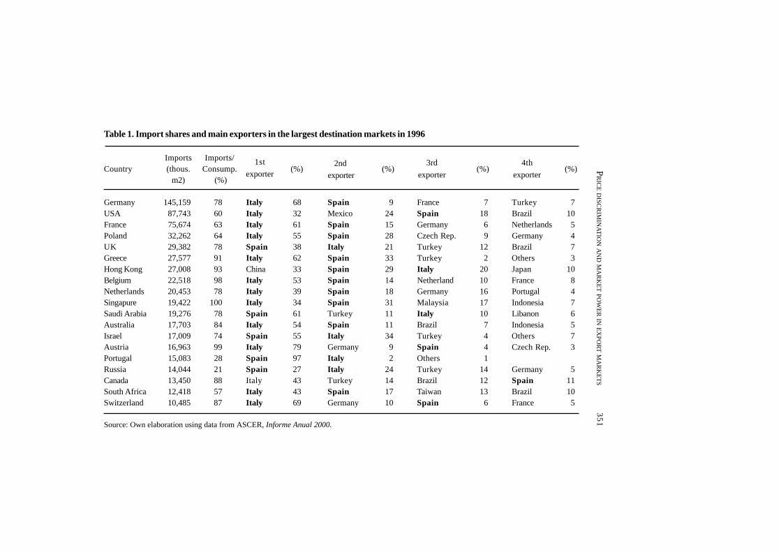
Table 1 displays the distribution of the ceramic tile exports among the 19 largest

destinations (accounting for 77% of world import market). Three features aboutthese export markets are worth mentioning since they have important implications

in the later empirical analysis. First, in almost all countries, imports represent more

than 60% of total domestic consumption, and the import/consumption ratio isabove 75% in the majority of cases. Second, in all but one market (Hong Kong),

either Italy or Spain is the largest exporter, and in fourteen of the nineteen markets

one of the two dominant exporting nations is also the second largest exporter.Furthermore, in all the destinations, the sum of Italian and Spanish products is

above 50% of total imports and, in some cases, the ratio is above 95% (Greece,

Israel and Portugal). Third, in almost every market, Italian and Spanish exporters

35

1 P

RIC

E DIS

CR

IMIN

ATIO

N AN

D MA

RK

ET P

OW

ER IN E

XP

OR

T MA

RK

ET

S

Table 1. Import shares and main exporters in the largest destination markets in 1996

Imports Imports/Country (thous. Consump. (%) (%) (%) (%)

m2) (%)

Germany 145,159 78 Italy 68 Spain 9 France 7 Turkey 7USA 87,743 60 Italy 32 Mexico 24 Spain 18 Brazil 10France 75,674 63 Italy 61 Spain 15 Germany 6 Netherlands 5Poland 32,262 64 Italy 55 Spain 28 Czech Rep. 9 Germany 4UK 29,382 78 Spain 38 Italy 21 Turkey 12 Brazil 7Greece 27,577 91 Italy 62 Spain 33 Turkey 2 Others 3Hong Kong 27,008 93 China 33 Spain 29 Italy 20 Japan 10Belgium 22,518 98 Italy 53 Spain 14 Netherland 10 France 8Netherlands 20,453 78 Italy 39 Spain 18 Germany 16 Portugal 4Singapure 19,422 100 Italy 34 Spain 31 Malaysia 17 Indonesia 7Saudi Arabia 19,276 78 Spain 61 Turkey 11 Italy 10 Libanon 6Australia 17,703 84 Italy 54 Spain 11 Brazil 7 Indonesia 5Israel 17,009 74 Spain 55 Italy 34 Turkey 4 Others 7Austria 16,963 99 Italy 79 Germany 9 Spain 4 Czech Rep. 3Portugal 15,083 28 Spain 97 Italy 2 Others 1Russia 14,044 21 Spain 27 Italy 24 Turkey 14 Germany 5Canada 13,450 88 Italy 43 Turkey 14 Brazil 12 Spain 11South Africa 12,418 57 Italy 43 Spain 17 Taiwan 13 Brazil 10Switzerland 10,485 87 Italy 69 Germany 10 Spain 6 France 5

Source: Own elaboration using data from ASCER, Informe Anual 2000.

1st

exporter2nd

exporter

3rd

exporter

4th

exporter


face competition from a neighbouring exporter group. Germany has a notable marketshare in the Netherlands, Austria and Switzerland while Turkey has a significant

presence in Greece and Saudi Arabia.

III. The theoretical framework

For a “normal” demand curve on an international market k in a particular periodt, X

kt = X

kt (P

kt, Z

t), the supply of tiles by a profit-maximising monopolistic exporter

selling to market k is given by the equilibrium output condition, where marginal

revenue equals marginal cost,

where Pk is the product price FOB in source country’s currency, ε

k is the price

elasticity of demand facing all firms in market k, and λ is the marginal cost ofproduction (all at time t). As written, it states that price in source country’s currency

is a mark-up over marginal cost determined by the elasticity of demand in the

destination market.

A. The pricing-to-market equation

Knetter (1989, 1993) showed that equation (1) can be approximated for cross-

section time series data by

J = I , S, (2)

where J refers to source country (here, Italy or Spain), k refers to each of the

destination markets and t refers to time. The export price to a specific marketbecomes a function of the bilateral exchange rate expressed as foreign currency

units per domestic currency, ekt; a destination-specific dummy variables, θ

k,

capturing time-invariant institutional features; and, a set of time dummies, λt, that

primarily reflects the variations in marginal costs of each exporter group. A random

disturbance term, ukt, is added to account for unobservable factors by the researcher,

or for measurement error in the dependent variable.4

tkt

ktktP λ

εε

−

=1

(1)

,lnln Jkt

Jt

Jk

Jkt

Jk

Jkt ueP +++= λθβ

4 Sullivan (1985) defined the conditions under which the use of industry-level data can be usedto make inferences about the extent of market segmentation using equation (1): (i) the industry

,


The advantage of the pricing-to-market (PTM) equation as an indicator ofimperfect competition is its simplicity and clear interpretation. First, if θ

k ≠ 0 the null

hypothesis of perfect competition in the export industry is rejected since the exporter

firm is able to fix different FOB prices for each destination; and, if βk ≠ 0 firms may

adjust their mark-ups as demand elasticities vary with respect to its local currency

price.5

A second advantage of the PTM equation is that it allows me to test forsimilarities in pricing behaviour between exporter groups in different source-

countries by comparing the β coefficients across destinations.

A third advantage of using the PTM equation is that I can incorporate a variablethat proxies time varying marginal costs for each exporter group, under the

assumptions that it is common to all destination markets. This measure is precise

when the elasticity of demand is constant so the mark-up is fixed over marginalcost. When the mark-up is sensitive to exchange rate changes and there is a

correlation between shocks to the cost function and the exchange rates, changes

in marginal costs will affect all prices equally so there is no idiosyncratic effect onprices, and the time effects will account for the impact of such shocks. In that case,

even when the time effects obtained from the PTM equation are not the marginal

costs exactly, “… there is no reason to think that they are biased measures ofmarginal cost, only noise ones” (Knetter 1989, p. 207).

has no influence over at least one factor that changes the supply price; (ii) there is littlevariation in the perceived elasticity of demand and in the marginal costs across firms selling inthe same destination market, and that (iii) no arbitrage opportunity exists across destinations.The three conditions are satisfied in the export markets of tiles. First, exchange rate variationis exogenous to the tile industry. Second, the cost of production differences across exporters arelikely to be small since ceramic tiles are produced with a standard technology in a single regionof each of the dominant exporting countries. Third, the physical characteristics of tiles makearbitrage highly unlikely.

5 The parameter βk has also an economic interpretation as the exchange rate pass-through

effect. On the one hand, a zero value for βk implies that the mark-up to a particular destination

is unresponsive to fluctuations in the value of the exporter’s currency against the buyer’s. Onthe other hand, the response of export prices to exchange rate variations in a setting ofimperfect competition depends on the curvature of the demand schedule faced by firms. As ageneral rule, when the demand becomes more elastic as local currency prices rise, the optimalmark-up charged by the exporter will fall as the importer’s currency depreciates. Negativevalues of βk

imply that exporters are capable of price discrimination and will try to offsetrelative changes in the local currency induced by exchange rate fluctuations. Thus, mark-upsadjust to stabilise local currency prices. Positive values of β

k suggest that exporters amplify the

effect of exchange rate fluctuations on the local currency price.


Once the cost structure of the competitors is ascertained, we are able to measurethe extent of competition in the export markets using the residual demand elasticity

approach.

B. The residual demand elasticity equation

How exchange rate shocks are passed through to prices in itself reveals littleabout the nature of competition in product markets. Indeed, the interpretation of

the PTM coefficients depends critically on the structure of the product market

examined (Goldberg and Knetter 1997). To assess the importance of market powerin the export industry, I directly measure the elasticity of the residual demand

curve of each exporter group.

The residual demand elasticity methodology was first developed by Baker andBresnahan (1988) to avoid the complexity of estimating multiple cross-price and

own-price demand elasticities in product differentiated markets. The residual

demand elasticity approach has the advantage of summarising the degree of marketpower of one producer in a particular market in a single statistic. Recently, Goldberg

and Knetter (1999) successfully applied a residual demand elasticity technique to

measure the extent of competition of the German beer and U.S. kraft paper industriesin international markets.

Consider two groups of exporters, Italians and Spaniards, selling in a particular

foreign market (therefore we omit the subindex k). The inverse demand curveincludes the export price of the other competitor and a vector of demand shifters,

J = I, S ; R = rival , (3)

where XJ stands for the total quantity exported by the J exporter group (note that

I use the letter J to refer to Italy or Spain and the letter R to refer to rival), P is theprice expressed in destination country’s currency terms, and Z is a vector of

exogenous variables affecting demand for tile exports. The supply relations for

each exporter group are

,´ JJ

JJJJ vDXeP += λ J = I, S, (4)

where λJ reflects the variations in marginal costs of each exporter group, D´J

is the partial derivative of the demand function with respect to XJ and v J is

a conduct parameter.The estimation of the market power of each exporter group requires the estimation

),,,( ZPXDP RJJ =


of the system of equations (3) and (4). A way to avoid estimating these equationssimultaneously is to estimate the so-called residual demand equation. The approach

does not estimate the individual cost, demand and conduct parameters, but it

captures their joint impact on market power through the elasticity of the residualdemand curve.

The first step in deriving the residual demand curve is to solve (3) and (4)

simultaneously for the price and quantities of the rival exporter group,

, J = I, S; R = rival. (5)

PR* is a partial reduced form; the only endogenous variable on the right-hand

side is XJ. The dependence of PR* and XJ arises because only the rivals’ producthas been solved out. By substituting PR* into (3), the residual demand for each

exporter group (J = I or S) is obtained:

J = I, S; R = rival. (6)

The residual demand curve has three observable arguments: the quantity

produced by the exporter group, the rival exporter group cost shifters and demand

shifters and one unobservable argument (the rivals’ conduct parameters).For each destination k, we can estimate a reduced form equation of the following

general form:

J=I, S; R= rival. (7)

Equation (7) is econometrically identified for each exporter group since cost

shifters for each exporter group are excluded arguments in their own residualdemand function. In each expression the only endogenous variable is the exported

quantity XJ. I can use both eJ and λJ as instruments since both variables affect the

exported supply of the exporter group in a particular destination independently ofother exporter groups competing in the same destination market. Exchange rate

shocks rotate the supply relation of the exporting group relative to other firms in

the market, helping us to identify the residual demand elasticity.Baker and Breshanan (1988) review the cases in which the residual demand

elasticity correctly measures the mark-up over marginal cost: Stackelberg leader

case, dominant firm model with competitive fringe, perfect competition, and marketswith extensive product differentiation. In other oligopoly models the equality

( )RRRJRR vZeXPP ,,,** λ=

( ),,,,),,( * RRRJRJJ vZeXRZPXDP λ==

,lnlnlnlnln ktktkRkt

Rk

Rkt

Rk

Jkt

Jk

Jk

Jkt vZeXP +++++= δλγβηα


between the relative mark-up and the estimated residual demand elasticity breaksdown. However, even in these cases, a steep residual demand curve is likely to be

a valid indicator of high degree of market power. In the ceramic tile industry, the

estimated residual demand elasticity may be a good approximation to the mark-ups, since the industry is characterised by substantial product differentiation, and

both source countries (especially Italy) have enjoyed a dominant position in the

world market.

IV. Data, estimation and results

A. The data

The data consist of quarterly observations from 1988:I to 1998:I on the valuesand quantities of ceramic tiles exports (Combined Nomenclature Code 690890)

from Spain and Italy to the largest market destinations. The prices of exports are

measured using FOB unit values. As far as I am aware, no country producesbilateral export price series, which is probably the main justification for the use of

unit value to measure bilateral export prices. The drawbacks of using unit values

as an approximation for actual transaction prices are well known. The most seriousproblems are the excessive volatility of the series and the effect on prices of

changes in product quality over time (Aw and Roberts 1988). However, any purely

random measurement error introduced by the use of unit values as a dependentvariable will only serve to reduce the statistical significance of the estimates.

The analysis includes sixteen export destinations (60 percent of world import

market): Germany, USA, France, United Kingdom, Greece, Hong-Kong, Belgium,Netherlands, Singapore, Australia, Israel, Austria, Portugal, Canada, South Africa

and Switzerland. Spanish and Italian exports represented between 48 and 99 percent

of total imports in each of these markets in 1996.6

The destination-specific exchange rate data refer to the end-of-quarter and is

expressed as units of the buyer’s currency per unit of the seller’s (unit of destination

market currency per home currency).As explained above, the exporter’s marginal cost function for ceramic tiles is

obtained directly from the estimation of the PTM equation. Demand for ceramic

tiles in each destination market is captured by two variables: building construction

6 Three large destination markets (Poland, Saudi Arabia and Russia) were excluded from ouranalysis due to data limitations.


and real private consumption expenditure. All the series in the empirical analysisare seasonally adjusted. An Appendix contains more details about the sources

and construction of the variables for the interested reader.

B. Evidence of pricing-to-market effects

In order to assess the potential for price discriminating behaviour on the partof Italian and Spanish exporters, I start by comparing the response of export prices

to exchange rate variations in each of the major destination markets. For a

comparable export product, differences in prices across export markets can beattributable to market segmentation. If the null of perfect competition is rejected,

price discrimination is possible so exporters may enjoy market power in those

destinations.Equation (2) is estimated by Zellner’s Seemingly Unrelated Regression

technique (Zellner 1962) to improve on efficiency by taking explicit account of the

expected correlation between disturbance terms associated with separate cross-section equations. The model is estimated with two different exchange rate

measures, the nominal exchange rate in foreign currency units per home currency,

and the nominal exchange rate adjusted by the wholesale/producer price index inthe destination market. The exchange rate adjustment is made, because the optimal

export price should be neutral to changes in the nominal exchange rate that

correspond to inflation in the destination markets. Estimated coefficients of thedestination-specific dummy variables, θ

k, reveal the average percentage difference

in prices across markets during the sample period, conditional on other controls

for destination-specific variation in those prices. In practice, only (N-1) separatevalues of θ

k can be estimated in the presence of a full set of time effects.

Consequently, I will normalise the model around West Germany, the world largest

import market, and test whether the fixed effects for the other countries aresignificantly different from zero. Results for the two source-countries, Italy and

Spain, are reported in Table 2. For each destination the Table reports the estimates

of the country effects θk and the coefficient on the exchange rate β

k.

Using either exchange rate measures, the destination specific effects are

significantly different from zero in almost all the cases.7 These results provide

evidence against the hypothesis of perfect competition. Looking at the estimated

7 F-tests for the exclusion of the country effects are overwhelmingly significant: 3486 for Italyand 4970 for Spain.


Table 2. Estimation of price discrimination across export markets

Foreign price adjusted nominal

exchange rate

Jkθ Jkβ J

kθ Jkβ

Destination k - source country J = Italy

Germany -0.59 (0.127)*** -0.53 (0.117)***

United States -0.34 (0.037)*** 0.15 (0.150) -0.32 (0.031)*** 0.12 (0.127)

France -0.09(0.032)*** -0.90 (0.132)*** -0.14 (0.028)*** -0.71 (0.104)***

UK -0.04 (0.032) -0.25 (0.230) -0.05 (0.029)* -0.26 (0.123)* *

Greece -0.41 (0.030)*** -0.54 (0.161)*** -0.35 (0.048)*** 0.08 (0.110)

Hong-Kong -0.45 (0.037)*** -0.07 (0.148) -0.45 (0.030)*** -0.03 (0.132)

Belgium -0.12 (0.032)*** -0.23 (0.125)* -0.11 (0.030)*** -0.23 (0.124)*

Netherland -0.08 (0.032)* * -0.57 (0.126)*** -0.09 (0.030)*** -0.58 (0.131)***

Singapore -0.33 (0.037)*** -0.07 (0.180) -0.34 (0.046)*** 0.03 (0.163)

Australia -0.16 (0.033)*** 0.00 (0.168) -0.14 (0.029)*** -0.10 (0.131)

Israel -0.51 (0.030)*** -0.40 (0.121)*** -0.62 (0.044)*** -0.37 (0.095)***

Austria -0.05 (0.032) -0.57 (0.127)*** -0.09 (0.050)*** -0.56 (0.127)***

Portugal -0.37 (0.030)*** -0.35 (0.246) -0.39 (0.032)*** -0.18 (0.081)* *

Canada -0.29 (0.040)*** 1.03 (0.261)*** -0.21 (0.028)*** 0.69 (0.161)***

South Africa -0.34 (0.033)*** -0.03 (0.137) -0.29 (0.036)*** -0.35 (0.134)***

Switzerland -0.02 (0.032) -0.22 (0.114)* -0.03 (0.030) -0.24 (0.122)*

Destination k - source country J = Spain.

Germany -0.69 (0.130)*** -0.68 (0.111)***

United States -0.29 (0.034)*** 0.21 (0.137) -0.28 (0.027)*** 0.08 (0.112)

France -0.04(0.030) -0.84 (0.134)*** -0.10 (0.024)*** -0.80 (0.095)***

UK -0.01 (0.029) -0.70 (0.183)*** -0.07 (0.025)*** -0.60 (0.107)***

Greece -0.45 (0.028)*** -0.12 (0.117) -0.44 (0.043)*** 0.03 (0.101)

Hong-Kong -0.42 (0.034)*** 0.04 (0.136) -0.41 (0.026)*** -0.03 (0.116)

Belgium 0.03 (0.030) -0.24 (0.128)* 0.04 (0.026)* -0.43 (0.118)***

Netherland 0.11 (0.030)*** -0.56 (0.128)*** 0.12 (0.026)*** -0.72 (0.124)***

Singapore -0.25 (0.033)*** 0.20 (0.158) -0.29 (0.039)*** 0.30 (0.136)* *

Australia -0.14 (0.030)*** 0.34 (0.148)* * -0.11 (0.025)*** 0.03 (0.116)

Israel -0.13 (0.027)*** 0.61 (0.091)*** -0.27 (0.038)*** 0.73 (0.083)***

Austria 0.19 (0.030)*** -0.56 (0.129)*** 0.20 (0.026)*** -0.72 (0.121)***

Portugal -0.11 (0.028)*** -0.10 (0.293) -0.16 (0.028)*** -0.29 (0.073)***

Nominal exchange rate


Canada -0.14 (0.036)*** -0.39 (0.222)* -0.17 (0.025)*** -0.37 (0.141)***

South Africa -0.24 (0.029)*** 0.92 (0.109)*** -0.22 (0.032)*** 0.81 (0.127)***

Switzerland 0.03 (0.029) 0.06 (0.112) 0.04 (0.027) 0.09 (0.115)

Note: SUR Estimation, N=41. *** , ** and * indicate significance at the 1%, 5% and 10% levelHeteroskedasticity robust standard errors in parenthesis. Exchange rate series are expressed asdestination market currency per source country currency and normalised to 1 in 1994:1.Wholesale price are used to adjust exchange rates.

Table 2. (Continued) Estimation of price discrimination across export markets

Foreign price adjusted nominal

exchange rate

Jkθ Jkβ J

kθ Jkβ

Nominal exchange rate

βk, the regression with nominal exchange rates indicates that 9 export markets for

Italy and 10 export markets for Spain violate the invariance of export prices toexchange rates implied by the constant-elasticity model (at 10 % significance level).

The regression with adjusted exchange rates increases the number of export markets

to 11 for Italy and 11 for Spain for the same significance level. There is evidence ofimperfect competition with constant elasticity of demand (θ

k ≠ 0 and β

k = 0) for

most non-European markets (see USA, Hong Kong, Singapore, Australia) in one

or another source-country. In most European destinations, tile exporters perceivedemand schedules to be more concave than a constant elasticity of demand (θ

k ≠

0 and βk < 0) revealing that exporters are able to price discriminate by offsetting the

relative price changes in the local currency price induced by exchange ratefluctuations. A plausible explanation is that tile exporters have an incentive for

price stabilization in the local currency in the European markets while there is a lack

of significant stabilisation across non-European markets. In other words, Europeandestinations are more competitive than non-European ones in the export tile

industry. Theories explaining PTM behaviour such as large fixed adjustment cost

differences across destinations (Kasa 1992) or concerns for market share varyingwith the size of the market (Froot and Klemperer 1989) seem unlikely to explain this

dichotomy in price behaviour. An alternative explanation could be the greater

price transparency in the European markets over the period 1988-1998, togetherwith the fact that the number of firms selling in the European markets is larger than

in the non-European markets. This interpretation coincides with the predictions of

the Cournot oligopoly model (Dornbusch 1987).


A surprising feature of our results is that destination-specific mark-upadjustment is very similar across source countries for each destination country. In

order to examine in more detail the pattern of price discrimination across destinations

we re-estimate Equation (2) under the assumption that βk = β across destination

markets (Knetter 1993). The t-statistics of the first row in Table 3 indicate that the

PTM coefficients are significantly different from zero for each exporter group. The

reported F-statistic reveals that the null hypothesis of identical PTM behaviouracross destination markets is rejected at the 5 percent level. The second row in

Table 3 offers a test of whether the identical PTM behaviour is supported across

only European destinations, leaving the non-European market coefficientsunconstrained. The last column of Table 3 offers pooled regression results. In it,

the constrained coefficients across destination markets for each source country

are additionally constrained to be the same for both source countries. The reportedF-statistic reveals that the null hypothesis of identical PTM behaviour across

source countries cannot be rejected at the 5 percent level. Therefore export price-

adjustment behaviour is different across the range of destination countries foreach source country but on aggregate both source countries have similar export

price-adjustment behaviour.

The results allow me to conclude that the export price-adjustment in responseto exchange rate variations is on average 30 percent, implying that more than half

of the exporter’s currency appreciation or depreciation are passed through to

import prices (after controlling for country-specific effects and time effects). Thelow sensitivity of domestic currency prices to changes in exchange rates provides

Table 3. Testing for identical pricing-to-market behaviour across destination

Italy Spain Pooled

Constrained βk

(all destinations) -0.256 (0.063)*** -0.304 (0.067)*** -0.292 (0.045)***

F-test F(15,584) = 21.52*** F(15,584) = 11.57*** F(1,599) = 0.46

Constrained βk

(Europe only) -0.281 (0.072)*** -0.401 (0.064)*** -0.337 (0.038)***

F-test F(8,584) = 8.41*** F(8,584) = 11.94*** F(1,592) = 2.14

Note: F-statistic tests the null hypothesis that PTM coefficient is the same across exportdestinations. For the pooled regression, F-statistics test the null that PTM coefficient is thesame for both source countries. *** indicates significance at the 1% level. Heteroskedasticityrobust standard errors in parenthesis.


indirect evidence of the existence of positive mark-ups in the export markets oftiles. The next questions to be addressed are how much market power each tile

producers has. To do that first I need an estimate of the marginal costs of each

exporter group.

C. Estimating marginal costs

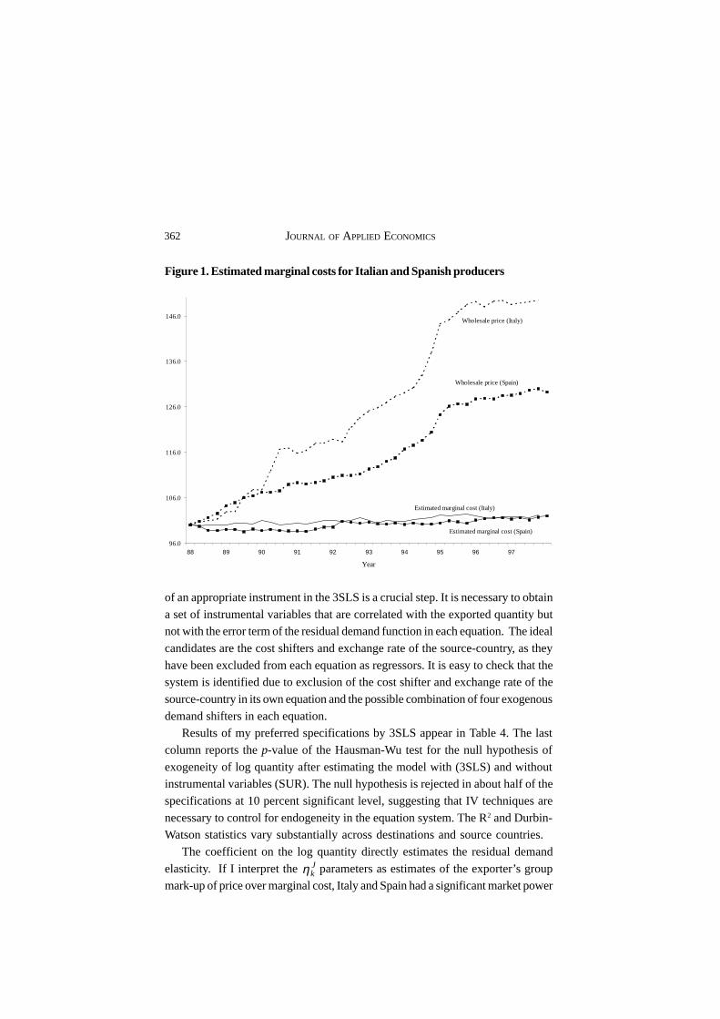
In this section, I present the estimates of the coefficients on the time dummy

variables, λt, which capture variations in marginal costs of exporters. Figure 1 plots

the indexes of the estimated time effects from the regression with price-level adjustedexchange rates for Italy and Spain.8 The estimated marginal costs of both exporter

groups are relatively flat over the sample and exhibit less volatility than producer

price indices, used in past studies to control for marginal cost changes.9 Therefore,if the time effects estimated in the PTM equation are better measures of the true

marginal cost changes, using producer price indices as a proxy probably

underestimate the role of mark-up adjustments in explaining the response of localcurrency prices of exports in relation to exchange rates changes (Knetter 1989).

D. Estimating the residual demand elasticities

Equation (7) is estimated for each of the destinations, k = 1,…16. Each equation

is in double log form so that the coefficients are elasticities. The cost shifterJtλ is

the estimated time effect of each exporter group J derived from the pricing-to-

market equations in the previous section. The demand shifters Zkt consist of a

combination of the construction index, real private consumption, the nominalexchange rate of a third competitor and a time trend.

If the exported quantity JktXln and its price are endogenously determined

through the residual demand function, then OLS provides biased and inconsistentestimates. Three-stage least squares (3SLS) is employed to estimate separately

each of the 16 systems of two equations. The exogeneity assumption of the exported

quantity is testable by comparing the 3SLS and seemingly unrelated regression(SUR) estimates using the Hausman-Wu test statistic (Hausman 1978). The choice

8 Although the estimated time effects have been normalised in Figure 1, the residual demandelasticity equation uses the actual estimated coefficients. The mean and standard deviationstatistics of the estimated time effects are (9.49, 0.070) for Italy and (6.97, 0.071) for Spain.

9 It is interesting to point out that our results are opposite to those of Knetter (1989) whofound that the estimated time effects trend upwards over the sample and exhibit higher volatility.


of an appropriate instrument in the 3SLS is a crucial step. It is necessary to obtain

a set of instrumental variables that are correlated with the exported quantity butnot with the error term of the residual demand function in each equation. The ideal

candidates are the cost shifters and exchange rate of the source-country, as they

have been excluded from each equation as regressors. It is easy to check that thesystem is identified due to exclusion of the cost shifter and exchange rate of the

source-country in its own equation and the possible combination of four exogenous

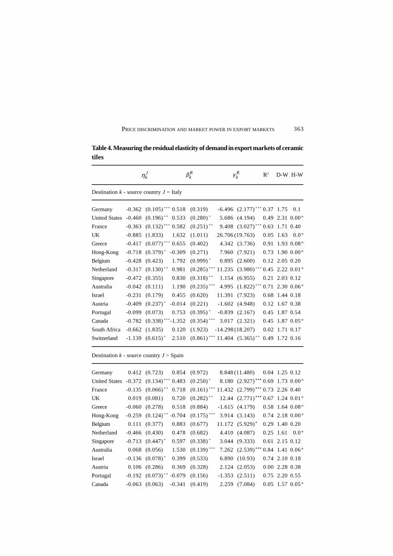
demand shifters in each equation.Results of my preferred specifications by 3SLS appear in Table 4. The last

column reports the p-value of the Hausman-Wu test for the null hypothesis of

exogeneity of log quantity after estimating the model with (3SLS) and withoutinstrumental variables (SUR). The null hypothesis is rejected in about half of the

specifications at 10 percent significant level, suggesting that IV techniques are

necessary to control for endogeneity in the equation system. The R2 and Durbin-Watson statistics vary substantially across destinations and source countries.

The coefficient on the log quantity directly estimates the residual demand

elasticity. If I interpret the Jkη parameters as estimates of the exporter’s group

mark-up of price over marginal cost, Italy and Spain had a significant market power

Figure 1. Estimated marginal costs for Italian and Spanish producers

96.0

106.0

116.0

126.0

136.0

146.0

88 89 90 91 92 93 94 95 96 97

Year

Wholesale price (Italy)

Wholesale price (Spain)

Estimated marginal cost (Italy)

Estimated marginal cost (Spain)


Table 4. Measuring the residual elasticity of demand in export markets of ceramictiles

Jkη Rkβ R

kγ R2 D-W H-W

Destination k - source country J = Italy

Germany -0.362 (0.105)* * * 0.518 (0.319) -6.496 (2.177)* * * 0.37 1.75 0.1

United States-0.460 (0.196)* * 0.533 (0.280)* 5.686 (4.194) 0.49 2.31 0.00 º

France -0.363 (0.132)* * * 0.582 (0.251)* * 9.408 (3.027)* * * 0.63 1.71 0.40

UK -0.885 (1.833) 1.632 (1.011) 26.706 (19.763) 0.05 1.63 0.0 º

Greece -0.417 (0.077)* * * 0.655 (0.402) 4.342 (3.736) 0.91 1.93 0.08 º

Hong-Kong -0.718 (0.379)* -0.309 (0.271) 7.960 (7.921) 0.73 1.90 0.00 º

Belgium -0.428 (0.423) 1.792 (0.999)* 0.895 (2.600) 0.12 2.05 0.20

Netherland -0.317 (0.130)* * 0.981 (0.285)* * * 11.235 (3.980)* * * 0.45 2.22 0.01 º

Singapore -0.472 (0.355) 0.830 (0.318)* * 1.154 (6.955) 0.21 2.03 0.12

Australia -0.042 (0.111) 1.190 (0.235)* * * 4.995 (1.822)* * * 0.71 2.30 0.06 º

Israel -0.231 (0.179) 0.455 (0.620) 11.391 (7.923) 0.68 1.44 0.18

Austria -0.409 (0.237)* -0.014 (0.221) -1.602 (4.948) 0.12 1.67 0.38

Portugal -0.099 (0.073) 0.753 (0.395)* -0.839 (2.167) 0.45 1.87 0.54

Canada -0.782 (0.338)* * * -1.352 (0.354)* * * 3.017 (2.321) 0.45 1.87 0.05 º

South Africa -0.662 (1.835) 0.120 (1.923) -14.298 (18.207) 0.02 1.71 0.17

Switzerland -1.139 (0.615)* 2.510 (0.861)* * * 11.404 (5.365)* * 0.49 1.72 0.16

Destination k - source country J = Spain

Germany 0.412 (0.723) 0.854 (0.972) 8.848 (11.480) 0.04 1.25 0.12

United States-0.372 (0.134)* * * 0.483 (0.250)* 8.180 (2.927)* * * 0.69 1.73 0.00 º

France -0.135 (0.066)* * 0.718 (0.161)* * * 11.432 (2.799)* * * 0.73 2.26 0.40

UK 0.019 (0.081) 0.720 (0.282)* * 12.44 (2.771)* * * 0.67 1.24 0.01 º

Greece -0.060 (0.278) 0.518 (0.884) -1.615 (4.179) 0.58 1.64 0.08 º

Hong-Kong -0.259 (0.124)* * -0.704 (0.175)* * * 3.914 (3.143) 0.74 2.18 0.00 º

Belgium 0.111 (0.377) 0.883 (0.677) 11.172 (5.929)* 0.29 1.40 0.20

Netherland -0.466 (0.430) 0.478 (0.682) 4.410 (4.087) 0.25 1.61 0.0 º

Singapore -0.713 (0.447)* 0.597 (0.338)* 3.044 (9.333) 0.61 2.15 0.12

Australia 0.068 (0.056) 1.530 (0.139)* * * 7.262 (2.539)* * * 0.84 1.41 0.06 º

Israel -0.136 (0.078)* 0.399 (0.533) 6.890 (10.93) 0.74 2.10 0.18

Austria 0.106 (0.286) 0.369 (0.328) 2.124 (2.053) 0.00 2.28 0.38

Portugal -0.192 (0.073)* * -0.079 (0.156) -1.353 (2.511) 0.75 2.20 0.55

Canada -0.063 (0.063) -0.341 (0.419) 2.259 (7.084) 0.05 1.57 0.05 º


South Africa -0.145 (0.092) 0.678 (0.251)* * * 3.032 (5.763) 0.60 1.57 0.17

Switzerland -0.009 (0.132) 1.174 (0.243)* * * 14.265 (5.144)* * * 0.65 1.52 0.16

Notes: Each destination is estimated jointly for Italy and Spain using 3SLS estimator. Dependentvariable: log-price of exports in local currency. Reported independent variables are log-quantityof exports, log-exchange rate between destination country and the direct rival country, andmarginal cost of direct rival country. Additional omitted exogenous variables may include theconstruction index, log-real private consumption, time trend and log-neighbour rival exchangerate in the destination market. *** , ** and * indicate significance at the 1%, 5% and 10% level.Standard errors are reported in parentheses. P-values reported for the Hausman-Wu test (H-W)test the endogeneity of log sales ,(ln JX J=I, S). º indicates p-value < 0.10.

Table 4. (Continued) Measuring the residual elasticity of demand in export marketsof ceramic tiles

Jkη Rkβ R

kγ R2 D-W H-W

over nine and six destinations respectively. For example, the residual demand

elasticity for Italy in the three largest markets is 0.362 (Germany), 0.460 (US) and0.363 (France) corresponding to a mark-up over marginal cost between 36 and 46

percent. Although Spain shows no market power in Germany, its residual demand

elasticity for US and France are 0.372 and 0.135, respectively. Looking at the rest ofthe destinations, Italy’s mark-up over marginal cost was on average 40 percent

while Spain’s were about 10 percent. This finding is consistent with Italy having a

leadership role in the industry.The interpretation of the rest of the coefficients in each equation is unclear

since they may reflect both direct effects on demand and indirect effects through

the adjustments of a rival exporter’s group; therefore I do not report them. Columns3 and 4 in Table 4 display the estimated coefficients of the rival’s adjusted exchange

rate and marginal costs. The positive sign of the coefficients reflects the significant

role of “outside” competition in constraining the market power of a particularexporter group. In general, the coefficients of the other exporter group’s exchange

rate and marginal costs are positive (and for some destinations significant),

indicating that the market power of one or another exporter group in most destinationmarkets is constrained by the presence of the other exporter group.10

10 When I estimated the residual demand elasticity equation using the wholesale price indexinstead of the estimated marginal cost obtained from the PTM equation, the sign of thesignificant coefficients for log-exchange rate and marginal cost of direct rival country did notchange. However, the magnitude of the estimated coefficient of the log-quantity of exports


Table 5. Relationship between residual demand elasticity and rivals’ market share

Spain Source

market country:

share Spain

Switzerland -1.139 6.2 13.0 Singapore -0.713 34.4 0.3

UK -0.885 38.3 21.5 Netherland -0.466 38.8 22.4

Canada -0.782 10.7 12.2 USA -0.372 31.8 39.9

Hong-Kong -0.718 29.3 7.4 Hong-Kong -0.259 20.0 7.4

South Africa -0.662 17.4 42.5 Portugal -0.192 1.9 72.4

Singapore -0.472 30.5 0.3 South Africa -0.145 43.1 42.5

USA -0.460 17.6 39.9 Israel -0.136 34.2 26.1

Belgium -0.428 14.1 2.1 France -0.135 61.2 36.8

Greece -0.417 32.8 9.4 Canada -0.063 43.1 12.2

Austria -0.409 3.8 1.5 Greece -0.060 62.1 9.4

France -0.363 15.3 36.8 Switzerland -0.009 69.2 13.0

Germany -0.362 8.5 22.3 UK 0.019 20.5 21.5

Netherland -0.317 18.1 22.4 Australia 0.068 54.4 16.2

Israel -0.231 54.8 26.1 Austria 0.106 79.3 1.5

Portugal -0.099 97.3 72.4 Belgium 0.111 52.8 2.1

Australia -0.042 10.9 16.2 Germany 0.412 67.7 22.3

Spearman correlation -0.15 -0.33 Spearman correlation -0.64 0.26

Pearson correlation -0.34 -0.30 Pearson correlation -0.51 0.09

Regression analysis b_Spain b_home Regression analysis b_Italy b_home

Rsq=0.13 -0.003 -0.002 Rsq=0.30 -0.007 -0.003

(0.004) (0.004) (0.003) (0.003)

Notes: Figures are obtained from Table 1 and Table 4. Market shares are for the year 1996.Figures in bold means p-value<0.10. In the regression analysis, standard errors are in parenthesis.

Source

country:

Italy

Residual

demand

Domestic

share

Domestic

share

Italy

market

share

Table 5 contains the final results of the two-step procedure used to estimate

the extent of competition in the destination markets of Italian and Spanish ceramictile exporters. Destination countries are ranked from the highest to the lowest

residual demand elasticities for each source country. If the market demand elasticities

are not very different across destinations, the residual demand elasticities measure

increased in many equations, suggesting on average greater mark-ups for both Italian andSpanish exporter groups across destination markets than the ones reported in Table 5.

Residual

demand


the degree of “outside” competition in each destination. To interpret the elasticities,note that the lower (in absolute value) the elasticity, the stronger the competition

that each exporter group faces from the other competitor. In the previous section

the PTM analysis showed that demand elasticities were constant for non-Europeandestinations and convex across European destinations. The rank correlations

between the market power of one exporter group and the market share of the other

exporter group are clearly negative with values of -0.34 for Italy and -0.51 for Spain,suggesting that the presence of competitors reduces the market power of the other

export group. A weaker correlation was also found between the market power of

one exporter group and the local producers’ domestic market share. In myregression analysis, reported in Table 5 (last rows), the coefficient of Italian market

share in the Spanish market power regression is negative and significant, while the

coefficient of Spanish market share in the Italian market power regression is negativebut not significant. The coefficient of domestic market share is negative but not

significant in both samples. Hence, Italian exports are strong substitutes of Spanish

tiles while the evidence is weaker in the opposite direction. Finally, domestic tilesseem to be poor substitutes for both Italian and Spanish tiles. A plausible

explanation behind these findings is the combined technological superiority and

design innovation that allow Italian and Spaniard tile makers to differentiatesuccessfully their products in the international markets.

V. Conclusions

Prior to 1987 Italian firms were the absolute world leaders in the production and

export of ceramic tiles. After 1988 the international market structure of the exportindustry changed as some developing countries attained large levels of domestically

orientated production, and Spanish producers gradually gained market quota in

the international export market.In order to characterise the market structure and conduct of Spanish and Italian

tile makers in each export market, I combine two different techniques borrowed

from the New Industrial Organisation (Bresnahan 1989). First, I measure thesensitivity of local currency prices of exported tiles to different countries with

respect to exchange rate changes. The so-called pricing-to-market equation permits

me to identify the existence of price discrimination and the similarity in the pricebehaviour of Italian and Spanish exporter groups across destination markets.

Second, I measure the response of one exporter group’s price to changes in the

quantity supplied, taking into account the supply response of the other rival


exporter group. The so-called residual demand elasticity equation allows me toidentify the extent of competition in the international tile market by quantifying the

sensitivity of the positive mark-ups of an exporter group across destinations with

respect to the market share of its rivals.Using the pricing-to-market equation I found that the export price-adjustment

in response to exchange rate variations was on average about 30%. I also observe

that both Spanish and Italian exporters set different prices in domestic currency todifferent destination markets. The evidence of market segmentation is weaker for

European destinations compared to non-European destinations, which could be

explained by the greater price transparency associated with economic integrationwithin Europe.

The estimation of the residual demand elasticity for each exporters’ group

revealed that, across destinations, both Italian and Spanish exporters have enjoyedpositive market power during the period examined (1988-1998). On average Italian

producers obtained mark-ups of 30 percent while Spanish mark-ups were 10 percent.

The results also reveal that Italian mark-ups are less sensitive to Spanishcompetition, while the historical leadership of Italian exporters has a depressive

effect on Spanish mark-ups in many destinations.

While the findings of this paper are most relevant to researchers studyingceramic tile industry, the methodology developed contributes more generally to

the literature testing market power in export markets. Obtaining information on the

determinants of the marginal costs such as input quantities or prices presents amajor problem for researchers interested in estimating market power in an industry.

I propose a simple solution to this problem by estimating the marginal cost for

each exporter group directly from the pricing-to-market equation. I also show thattechniques developed in one-source-country/multiple-destination can be

implemented to multiple-source-countries/multiple-destinations. My current

agenda of research includes explicitly modelling the strategic behaviour betweenexporter groups for a better understanding of export pricing policies in different

periods of time, in a similar way as Kadayali (1997) did for the US photographic film

industry or Gross and Schmitt (2000) did for the Swiss automobile market.


Appendix

A. Export quantities and prices

Price and quantity of ceramic tiles exports came from national customs, who

collected data on the total number of squared metres and the total national currency

value of exports of ceramic tiles to each destination country. Data were kindlyprovided by Assopiastrelle and Ascer, the two national entrepreneur associations.

To ensure homogeneity in the product I selected the product registered as “CN

Code 690890” from the Eurostat-Comext Customs Cooperation CouncilNomenclature: “Glazed flags and paving, hearth or wall tiles of stone ware,

earthenware or fine pottery,..., with a surface of above 7cm2”. The value of exports

does not include tariff levies, the cost of shipping and other transportation costs.Monthly data were available for all European destinations, but Italian series for

non-European destinations are only collected on a quarterly basis. Unit values are

quarterly average prices constructed dividing the value by the quantity of tradeflows. For the monthly series unit values for each quarter were calculated as the

mean average of the corresponding three months. I reduced the volatility of the

unit values series by eliminating potential outliers, excluding in my calculationsthe monthly prices five times larger or smaller than the standard deviation of the

annual average in the corresponding year (accounting for 1% of the destination-

quarter observations in the Spanish and Italian data).

B. Exchange rates and demand variables

The data on exchange rate and wholesale price were collected from the

International Financial Statistics of the International Monetary Fund (IMF). The

destination-specific exchange rate data refer to the end-of-quarter and are expressedas units of the buyer’s currency per unit of the seller’s. The adjusted nominal

exchange rate is nominal exchange rate divided by the destination market wholesale

price level.I use quarterly data on “new building construction permits” as an indicator of

building construction demand. Data were obtained from DATASTREAM and the

original sources are OECD and National Statistics. Since some series are notavailable for all the countries, alternative proxies were utilised. Specifically, the

“Construction in GDP” for Italy and South Africa, “Work put in construction” for

Hong Kong and Austria, and the “Construction production index” for Israel. Real


private consumption expenditures were used to proxy for the household demandof ceramic tiles. When disaggregated data were unavailable gross domestic

production data were employed. The data were obtained from International

Financial Statistics (IMF). All the series are seasonally adjusted.

References

Aw, Bee-Yan, and Mark Roberts (1998), "Price and quality comparisons for the US

footwear imports: An application of multilateral index numbers", in R.E. Feenstra,

ed., Empirical Methods for International Trade, Cambridge, MA, MIT Press.Aw, Bee-Yan (1993), "Price discrimination and markups in export markets", Journal

of Development Economics 42: 315-36.

Baker, Jonathan B., and Timothy F. Bresnahan (1998), "Estimating the residualdemand curve facing a single firm", International Journal of Industrial

Economics 6: 283-300.

Bernstein, Jeffrey I. and Pierre A. Mohen (1994), "Exports, margins and productivitygrowth: With an application to Canadian industries", Canadian Journal of


Bresnahan, Timothy F. (1989), "Empirical methods for industries with market power",in S. Richard and R. D. Willig, eds., Handbook of Industrial Organization,

Amsterdam, North Holland.

Bughin, Jacques (1996), "Exports and capacity constraints", Journal of Industrial

Economics 48:266-78.

Dornbusch, Rudiger (1987), "Exchange rates and prices", American Economic

Review 59: 93-106.Froot, Kenneth, and Paul Klemperer (1989), "Exchange rate pass-through when

market share matters", American Economic Review 79: 637-54.

Gil-Pareja, Salvador (2002), "Export price discrimination in Europe and exchangerates", Review of International Economics 10: 299-312

Goldberg, Penelopi K., and Michael M. Knetter (1997), "Goods, prices, and exchange

rates: What we have learned?", Journal of Economic Literature 35: 1243-1272.Goldberg, Penelopi K., and Michael M. Knetter (1999), "Measuring the intensity

of competition in export markets", Journal of International Economics 47:27-

60.Gross, Dominique M., and Nicolas Schmitt (2000), "Exchange rate pass-through

and dynamic oligopoly: An empirical investigation", Journal of International



Hausman, Jerry (1978), "Specification tests in econometrics", Econometrica 46:1251-1272.

Kadayali, Vrinda (1997), "Exchange rate pass through for strategic pricing and

advertising: An empirical analysis of the US photographic film industry", Journal

of International Economics 43: 1-26.

Knetter, Michael M. (1989), "Price discrimination by US and German exporters",

American Economic Review 79: 198-210.Knetter, Michael M. (1993), "International comparisons of pricing to market

behaviour", American Economic Review 83: 473-86.

Porter, Michael E. (1990), The Competitive Advantage of Nations, The Free Press.Sullivan, Dan (1985), "Testing hypothesis about firm behaviour in the cigarette

industry", Journal of Political Economy 93: 586-98.

Steen, Frode, and Kjell J. Salvanes (1999), "Testing for market power using adynamic oligopoly model", International Journal of Industrial Economics

17:147-77.

Yerger, David B. (1996), "Testing for market power in multi-product industriesacross multiple export markets", Southern Economic Journal 62: 938-56.

Zellner, Andreas (1962), "An efficient method of estimating seemingly unrelated

regressions and tests for aggregation bias", Journal of the American Statistical

Association 57: 348-68.

price discrimination and market power …ageconsearch.umn.edu/bitstream/37143/2/requena.pdf · *...

Documents