Draft version February 7, 2010Preprint typeset using LATEX style emulateapj v. 11/26/04

DISSECTING THE GRAVITATIONAL LENS B1608+656. II. PRECISION MEASUREMENTS OF THE HUBBLECONSTANT, SPATIAL CURVATURE, AND THE DARK ENERGY EQUATION OF STATE*

S. H. Suyu1, P. J. Marshall2,3, M. W. Auger3,4, S. Hilbert1,5, R. D. Blandford2, L. V. E. Koopmans6,C. D. Fassnacht4, and T. Treu3,7

Draft version February 7, 2010

ABSTRACT

Strong gravitational lens systems with measured time delays between the multiple images providea method for measuring the “time-delay distance” to the lens, and thus the Hubble constant. Wepresent a Bayesian analysis of the strong gravitational lens system B1608+656, incorporating (i)new, deep Hubble Space Telescope (HST) observations, (ii) a new velocity dispersion measurement of260± 15 km s−1 for the primary lens galaxy, and (iii) an updated study of the lens’ environment. Ouranalysis of the HST images takes into account the extended source surface brightness, and the dustextinction and optical emission by the interacting lens galaxies. When modeling the stellar dynamicsof the primary lens galaxy, the lensing effect, and the environment of the lens, we explicitly include thetotal mass distribution profile logarithmic slope γ′ and the external convergence κext; we marginalizeover these parameters, assigning well-motivated priors for them, and so turn the major systematicerrors into statistical ones. The HST images provide one such prior, constraining the lens massdensity profile logarithmic slope to be γ′ = 2.08 ± 0.03; a combination of numerical simulations andphotometric observations of the B1608+656 field provides an estimate of the prior for κext: 0.10+0.08

−0.05.This latter distribution dominates the final uncertainty on H0. Fixing the cosmological parameters atΩm = 0.3, ΩΛ = 0.7, and w = −1 in order to compare with previous work on this system, we find H0 =70.6+3.1

−3.1 km s−1 Mpc−1. The new data provide an increase in precision of more than a factor of two,even including the marginalization over κext. Relaxing the prior probability density function for thecosmological parameters to that derived from the WMAP 5-year data set, we find that the B1608+656data set breaks the degeneracy between Ωm and ΩΛ at w = −1 and constrains the curvature parameterto be −0.031 < Ωk < 0.009 (95% CL), a level of precision comparable to that afforded by the currentType Ia SNe sample. Asserting a flat spatial geometry, we find that, in combination with WMAP,H0 = 69.7+4.9

−5.0 km s−1 Mpc−1 and w = −0.94+0.17−0.19 (68% CL), suggesting that the observations of

B1608+656 constrain w as tightly as do the current Baryon Acoustic Oscillation data.Subject headings: cosmology: observations — distance scale — galaxies: individual (B1608+656) —

gravitational lensing: strong — methods: data analysis

1. INTRODUCTION

The Hubble constant (H0, measured in units ofkm s−1 Mpc−1) is one of the key cosmological parame-ters since it sets the present age, size, and critical densityof the Universe.

Methods for measuring the Hubble constant includeType Ia supernovae (SNe Ia) (e.g. Tammann 1979; Riesset al. 2009), the Sunyaev-Zel’dovich effect (e.g. Sunyaev& Zel’dovich 1980; Bonamente et al. 2006), the expand-

* Based in part on observations made with the NASA/ESA Hub-ble Space Telescope, obtained at the Space Telescope Science In-stitute, which is operated by the Association of Universities forResearch in Astronomy, Inc., under NASA contract NAS 5-26555.These observations are associated with program GO-10158.

1 Argelander-Institut fur Astronomie, Auf dem Hugel 71, 53121Bonn, Germany

2 Kavli Institute for Particle Astrophysics and Cosmology, Stan-ford University, PO Box 20450, MS 29, Stanford, CA 94309, USA

3 Department of Physics, University of California, Santa Bar-bara, CA 93106-9530, USA

4 Department of Physics, University of California at Davis, 1Shields Avenue, Davis, CA 95616, USA

5 Max-Planck-Institut fur Astrophysik, Karl-Schwarzschild-Str.1, 85741 Garching, Germany

6 Kapteyn Astronomical Institute, P.O. Box 800, 9700AVGroningen, The Netherlands

7 Sloan Fellow, Packard FellowElectronic address: suyu@astro.uni-bonn.de

ing photosphere method for Type II supernovae (e.g. Kir-shner & Kwan 1974; Schmidt et al. 1994), and maserdistances (e.g. Herrnstein et al. 1999; Macri et al. 2006).However, perhaps the two most well-known recent mea-surements come from the Hubble Space Telescope (HST)Key Project (KP) (Freedman et al. 2001) and the Wilkin-son Microwave Anisotropy Probe (WMAP) observationsof the cosmic microwave background (CMB) (e.g. Ko-matsu et al. 2009). The HST KP measurement of H0 isbased on secondary distance indicators (including TypeIa supernovae, Tully-Fisher, surface brightness fluctua-tions, Type II supernovae, and the fundamental plane)that are calibrated using Cepheid distances to nearbygalaxies with a zero point in the Large Magellanic Cloud.The resulting Hubble constant is 72 ± 8 km s−1 Mpc−1

(Freedman et al. 2001). We note that the largest con-tributor to the systematic error from the distance lad-der of which this measurement depends is the metallicitydependence of the Cepheid period-luminosity relation.More recently, Riess et al. (2009) addressed some of thesesystematic effects with an improved differential distanceladder using Cepheids, SNe Ia, and the maser galaxyNGC 4258, finding H0 = 74.2 ± 3.6 km s−1 Mpc−1, a 5%local measurement of Hubble’s constant.

The five year measurement made usingWMAP temperature and polarization data is

2 Suyu et al.

H0 = 71.9+2.6−2.7 km s−1 Mpc−1 (Dunkley et al. 2009),

under the assumption that the Universe is flat andthat the dark energy is described by a cosmologicalconstant (with equation of state parameter w = −1).The uncertainty in H0 increases markedly if either ofthese two assumptions is relaxed, due to degeneracieswith other cosmological parameters. For example,WMAP gives H0 ∼ 50 km s−1 Mpc−1 without theflatness assumption, and H0 = 74+15

−14 km s−1 Mpc−1 fora flat Universe with time-independent w not fixed atw = −1. As H0 is such an important parameter, it isessential to measure it using multiple methods. In thispaper, we use a single strong gravitational lens as anindependent probe of H0, and explore its systematicerrors and relations with other cosmological parametersto provide guidance for future studies. We will showthat the single lens is competitive with those of thebest current cosmographic probes. Given the currentprogress in measuring time delays (e.g., Vuissoz et al.2007, 2008; Paraficz et al. 2009), the methodology inthis paper should lead to substantial advances whenapplied to samples of gravitational lenses.

Strong gravitational lensing occurs when a sourcegalaxy is lensed into multiple images by a galaxy lyingalong its line of sight. The principle of using strong grav-itational lens systems with time-variable sources to mea-sure the Hubble constant is well understood (e.g. Refs-dal 1964, Schneider, Kochanek, & Wambsganss 2006).The relative time delays between the multiple images areinversely proportional to H0 via a combination of angu-lar diameter distances and depend on the lens potential(mass) distribution. We refer to the combination of angu-lar diameter distances as the “time-delay distance”. Bymeasuring the time delays and modeling the lens poten-tial, one can infer the value for the time-delay distance;this distance-like quantity is primarily sensitive to H0

but depends also on other cosmological parameters whichmust be factored into the analysis. The direct measure-ment of the time-delay distance means that gravitationallensing is independent of distance ladders.

Despite being an elegant method, gravitational lens-ing has its limitations. Perhaps the most well-known isthe “mass-sheet degeneracy” between H0 and externalconvergence (Falco, Gorenstein, & Shapiro 1985). Thereis also a degeneracy between H0 and the slope of thelens mass distribution, especially for lenses where theconfiguration is nearly symmetric (e.g. Wucknitz 2002).In such cases, the image positions are at approximatelythe same radial distance from the lens center and so theslope is poorly constrained. In both cases the remedy isto provide more information. Modeling the mass envi-ronment of the lens can, in principle, independently con-strain the external convergence (e.g., Keeton & Zablud-off 2004; Fassnacht et al. 2006a; Blandford et al. in prepa-ration); likewise, lens galaxy stellar velocity dispersionmeasurements (e.g., Grogin & Narayan 1996a,b; Tonry& Franx 1999; Koopmans & Treu 2002; Treu & Koop-mans 2002; Barnabe & Koopmans 2007; McKean et al.2009) and analysis of any extended images (e.g., Dye &Warren 2005; Dye et al. 2008) can constrain the massdistribution slope.

A measurement of H0 to better than a few percentprecision would provide the single most useful comple-ment to results obtained from studies of the CMB for

dark energy studies (e.g. Hu 2005; Riess et al. 2009).Dark energy has been used to explain the acceleratingUniverse, discovered using luminosity distances to SNeIa (Riess et al. 1998; Perlmutter et al. 1999). Efforts instudying dark energy often characterize it by a constantequation of state parameter w (where w = −1 corre-sponds to a cosmological constant) and assume a flatUniverse. These include Perlmutter et al. (1999), who intheir Figure 10 constrained w . −0.65 for present daymatter density values of Ωm ≥ 0.2, and Eisenstein et al.(2005), who combined their angular diameter distancemeasurement to z = 0.35 from Baryon Acoustic Oscilla-tions (BAO) with WMAP data (Spergel et al. 2007) toobtain w = −0.80±0.18. Recently, Komatsu et al. (2009)measured w = −0.992+0.061

−0.062 by combining WMAP 5-yearresults (WMAP5) with observations of SNe Ia (Kowalskiet al. 2008) and BAO (Percival et al. 2007). Komatsuet al. (2009) also explored more general dark energy de-scriptions. In our study, we combine the time-delay dis-tance measurement from B1608+656 with WMAP datato derive a constraint on w, and compare the constrain-ing power of B1608+656 to that of other cosmographicprobes.

In this paper, we present an accurate measurement ofH0 from the gravitational lens B1608+656. A compre-hensive lensing analysis of the lens system is in a com-panion paper (Paper I; Suyu et al. 2009). Using the re-sults from Paper I, we focus in this paper on techniquesrequired to break the mass-sheet degeneracy in order toinfer a value of H0 with well-understood uncertainty. Wethen explore the influence of this measurement on othercosmological parameters.

The organization of the paper is as follows. In Section2, we briefly review the theory behind using gravitationallenses to measure H0, include a description of the mass-sheet degeneracy, and describe the dynamics modelingfor the measured velocity dispersion. In Section 3, weoutline the probability theory for combining various datasets and for including cosmological priors. In Section 4,we present the gravitational lens B1608+656 as a can-didate for measuring H0, and show the lens modelingresults. We present the new velocity dispersion measure-ment and the stellar dynamics modeling in Section 5.The study of the convergence accumulated along the lineof sight to B1608+656 is discussed in Section 6. The pri-ors for our model parameters are described in Section 7.Finally, in Section 8 we combine the lensing, dynamicsand external convergence analyses to break the mass-sheet degeneracy and infer H0 from the B1608+656 dataset. We then show how B1608+656 aids in constrainingflatness and measuring w when combined with WMAP,before concluding in Section 9.

Throughout this paper, we assume a w-CDM universewhere dark energy is described by a time-independentequation of state with parameter w = P/ρc2 with presentday dark energy density ΩΛ, and the present day matterdensity is Ωm. Each quoted parameter estimate is themedian of the appropriate one-dimensional marginalizedposterior probability density function (PDF), with thequoted uncertainties showing, unless otherwise stated,the 16th and 84th percentiles (that is, the bounds of a68% confidence interval).

Cosmological constraints from gravitational lens B1608+656 3

2. MEASURING H0 USING LENSING, STELLARDYNAMICS, AND LENS ENVIRONMENT STUDIES

In this section we briefly review the theory of gravita-tional lensing forH0 measurement (Section 2.1), describethe mass-sheet degeneracy (Section 2.2), and present thedynamics modeling (Section 2.3). Readers familiar withthese subjects can proceed directly to Section 3.

2.1. Theory of gravitational lensing

For a strong lens system in an otherwise homogeneousRobertson-Walker universe, the excess time delay of an

image at angular position ~θ = (θ1, θ2) with corresponding

source position ~β = (β1, β2) relative to the case of nolensing is

t(~θ, ~β) =1

c

DdDs

Dds(1 + zd)φ(~θ, ~β), (1)

where zd is the redshift of the lens, φ(~θ, ~β) is the so-calledFermat potential, and Dd, Ds, and Dds are, respectively,the angular diameter distance from us to the lens, fromus to the source, and from the lens to the source. TheFermat potential is defined as

φ(~θ, ~β) ≡[

(~θ − ~β)2

2− ψ(~θ)

]

, (2)

where the first term comes from the geometric path dif-ference as a result of the strong lens deflection, and thesecond term is the gravitational delay described by the

lens potential ψ(~θ). The scaled deflection angle of a light

ray is ~α(~θ) = ~∇ψ(~θ), and the lens equation that governs

the deflection of light rays is ~β = ~θ − ~α(~θ).

The projected dimensionless surface mass density κ(~θ)is

κ(~θ) =1

2∇2ψ(~θ), (3)

where

κ(~θ) =Σ(Dd

~θ)

Σcrwith Σcr =

c2Ds

4πGDdDds, (4)

and Σ(Dd~θ) is the physical projected surface mass den-

sity.The constant coefficient in Equation (1) is proportional

to the angular diameter distance and hence inversely pro-portional to the Hubble constant. We can thus simplifyEquation (1) to the following:

t(~θ, ~β)=D∆t

cφ(~θ, ~β) (5)

∝ 1

H0φ(~θ, ~β), (6)

where D∆t ≡ (1 + zd)DdDs/Dds is referred to as thetime-delay distance.

Therefore, by modeling the lens potential (ψ(~θ)) and

the source position (~β), we can use time-delay lens sys-tems to deduce the value of the Hubble constant, andindeed the other cosmological parameters that appearin D∆t. In this way, strong lensing can be seen as akinematic probe of the universal expansion, in the samegeneral category as SNe Ia and BAO. Since the princi-pal dependence of D∆t is on H0, we continue to discuss

lenses as a probe of this one parameter; however, we shallsee that the other cosmological parameters play an im-portant role in the analysis.

Gravitational lens systems with spatially extendedsource surface brightness distributions are of special in-terest since they provide additional constraints on thelens potential. However, in this case, simultaneous de-terminations of the source surface brightness and the lenspotential are required.

2.2. Mass-sheet degeneracy

We now briefly describe the mass-sheet degeneracy andits relevance to this research (see e.g. Falco et al. 1985;Schneider et al. 2006, for details). As its name suggests,this is a degeneracy in the mass modeling correspond-ing to the addition of a mass sheet that contributes aconvergence and zero shear (and a matching scaling ofthe original mass distribution) which leaves the predictedimage positions unchanged. A circularly symmetric sur-face mass density distribution that is uniform interiorto the line of sight is one example of such a lens. Sup-

pose we have a lens model κmodel(~θ) that fits the ob-servables of a lens system (i.e., image positions, flux ra-tios for point sources, and the image shapes for extendedsources). A new model described by the transformation

κtrans(~θ) = λ + (1 − λ)κmodel(~θ), where λ is a constant,would also fit the lensing observables equally well. Theparameter λ corresponds physically to the convergenceof the sheet. Since we might think of including exactlysuch a parameter to account for additional physical masslying along the line of sight, or in the lens plane to modela nearby group or cluster, it is clear that the mass-sheetdegeneracy corresponds to a degeneracy between this ex-ternal convergence (κext) and the mass normalization ofthe lens galaxy.9

Despite the invariance of the image positions, shapesand relative fluxes under a mass-sheet transforma-tion, the relative Fermat potential between the im-

ages changes according to ∆φtrans(~θ, ~βtrans) = (1 −λ)∆φmodel(~θ, ~βmodel). Therefore, given measured relativetime delays ∆t, which are inversely proportional to H0

and proportional to the relative Fermat potential (Equa-tion 6), the transformed model κtrans would lead to anH0 that is a factor (1 − λ) lower than that of the ini-tial κmodel (for fixed Ωm, ΩΛ, and w). In other words, ifthere is physically any external convergence κext due tothe lens’ local environment or mass structure along theline of sight to the lens system that is not incorporatedin the lens modeling, then

Htrue0 = (1 − κext)H

model0 . (7)

This degeneracy is present because lensing observa-tions only deliver relative positions and fluxes. The de-generacy can be broken, allowing us to measure H0, if (i)we know the magnitude or angular size of the source inabsence of lensing, (ii) we have information on the massnormalization of the lens, or (iii) we can compare the

9 To be specific, the prescription that we adopt for combiningthe effects of many mass sheets at redshifts zi with surface mass

densities Σi is κext = 4πG

c2

X

i

Σi(Di~θ)DiDis

Ds.

4 Suyu et al.

measured shear in the lens with the observed distribu-tion of mass to calibrate κext. For most of the stronglens systems including B1608+656, case (i) does not ap-ply, so circumventing the mass-sheet degeneracy requiresthe input of more information, either about the lensinggalaxy itself, or its three-dimensional environment. Wedistinguish between two kinds of mass sheets: internaland external. Internal mass sheets, which are physicallyassociated with the lens galaxy, are due to nearby, phys-ically associated galaxies, groups or clusters which, cru-cially, affect the stellar dynamics of the lens galaxy. Ex-ternal mass sheets describe mass distributions that arenot physically associated with the lens galaxy and, bydefinition, do not affect the stellar dynamics. Typicallythese will lie along the line of sight to the lens (Fassnachtet al. 2006a). We identify κext as the net convergence ofthis external mass sheet.

Two methods for breaking the mass-sheet degeneracyare then:

i. Stellar dynamics of the lens galaxy. Stellar dy-namics can be used jointly with lensing to breakthe internal mass-sheet degeneracy by providingan estimate of the enclosed mass at a radius dif-ferent from the Einstein radius, which is approxi-mately the radius of the lensed images from the lensgalaxy (e.g., Grogin & Narayan 1996a,b; Tonry &Franx 1999; Koopmans & Treu 2002; Treu & Koop-mans 2002; Barnabe & Koopmans 2007). We notethat for a given stellar velocity dispersion, thereis a degeneracy in the mass and the stellar orbitanisotropy (which characterizes the amount of tan-gential velocity dispersion relative to radial disper-sion). Nonetheless, the mass-isotropy degeneracyis nearly orthogonal to the mass-sheet degeneracy,so a combination of the mass within the effectiveradius (from the stellar velocity dispersion) and themass within the Einstein radius (from lensing) ef-fectively breaks both the mass-isotropy and the in-ternal mass-sheet degeneracies. We describe howthis works within the context of our chosen massmodel in Section 2.3 below.

ii. Studying the environment and the line of sight tothe lens galaxy. Observations of the field aroundlens galaxies allow a rough picture of the projectedmass distribution to be built up. Many lens galax-ies lie in galaxy groups, which can be identified ei-ther by their spectra or, more cheaply (but less ac-curately), by their colors and magnitudes. By mod-eling the mass distribution of the groups and galax-ies in the lens plane and along the line of sight tothe lens galaxy, one can estimate the external con-vergence κext at the redshift of the lens (e.g. Mom-cheva et al. 2006; Fassnacht et al. 2006a; Augeret al. 2007, and references therein). The groupmodeling requires (i) identification of the galaxiesthat belong to the group of the lens galaxy, and (ii)estimates of the group centroid and velocity disper-sion. A number of recipes can be followed. For ex-ample, Keeton & Zabludoff (2004) considered twoextremes: (i) the group is described by a singlesmooth mass distribution, and (ii) the masses areassociated with individual galaxy group members

with no common halo. The realistic mass distri-bution for a galaxy group should be somewherebetween these two extremes. The experience todate is that modeling lens environments accuratelyis very difficult, with uncertainties of 100% typical(e.g. Momcheva et al. 2006; Fassnacht et al. 2006a).In Section 6, we describe an alternative approachfor quantifying the external convergence in a statis-tical manner: ray-tracing through numerical simu-lations of large-scale structure (Hilbert et al. 2007).In this section we also present a first attempt attailoring the ray-tracing results to our one line ofsight, using the relative galaxy number counts inthe field.

We emphasize that the mass-sheet degeneracy is sim-ply one of the several parameter degeneracies in the lensmodeling that has been given a special name. Whenpower-laws (κ ∼ bR1−γ′

, where R is the radial distancefrom the lens center, b is the normalization of the lens,and γ′ is the radial slope in the mass profile) are used todescribe the lens mass distribution, one often finds a H0-γ′ degeneracy in addition to the H0-b-κext (mass-sheet)degeneracy (for fixed Ωm, ΩΛ and w; more generally,D∆t

would be in place of H0). These two degeneracies are ofcourse related via H0. The H0-γ

′ degeneracy primarilyoccurs in lens systems with symmetric configurations dueto a lack of information on γ′. In contrast, lens systemswith images spanning a range of radii or with extendedimages provide information on γ′ (e.g. Wucknitz et al.2004; Dye et al. 2008), and so the H0-γ

′ degeneracy isbroken. Nonetheless, the H0-b-κext degeneracy is stillpresent unless we provide information from dynamics andlens environment studies.

2.3. Stellar dynamics modeling

In order to model the velocity dispersion of the starsin the lens galaxy, we need a model for the local grav-itational potential well in which those stars are orbit-ing. This potential is due to both the mass distributionof the lens galaxy, and also the “internal mass sheet”due to neighboring groups and galaxies physically asso-ciated with the lens, as described in the previous sub-section. Recent studies such as the Sloan Lens ACSSurvey (SLACS) and hydrostatic X-ray analyses foundthat the sum of these internal components can be well-described by a power law (e.g. Treu et al. 2006; Koop-mans et al. 2006; Gavazzi et al. 2007; Koopmans et al.2009; Humphrey & Buote 2009). With this in mind, weassume that the total (lens plus sheet) mass density dis-tribution is spherically symmetric and of the form

ρlocal = ρ0

(r0r

)γ′

, (8)

where γ′ is the logarithmic slope of the effective lens den-

sity profile, and ρ0rγ′

0 is the normalization of the massdistribution that is determined quite precisely by thelensing, up to a small offset contributed by the externalconvergence κext. This normalization can be expressedin terms of observable or inferrable quantities as we showbelow.

By integrating ρlocal within a cylinder with radius given

Cosmological constraints from gravitational lens B1608+656 5

by the Einstein radius REin, we find

Mlocal =4π

∫ ∞

0

dz

∫ REin

0

ρ0rγ′

0

s ds

(s2 + z2)γ′/2(9)

=−ρ0rγ′

0

π3/2Γ(γ′−32 )R3−γ′

Ein

Γ(γ′

2 ). (10)

However, the mass responsible for creating an Einsteinring is a combination of this local mass and the externalmass contributed along the line of sight, so the masscontained within the Einstein ring is

MEin = Mlocal +Mext (11)

where MEin is the mass enclosed within the Einstein ra-dius REin that would be inferred from lensing,10 givenby

MEin = πR2EinΣcr, (12)

and Mext is the mass contribution from κext,

Mext = πR2EinκextΣcr. (13)

Combining Equations (10), (11), (12), and (13), we find

ρ0rγ′

0 = (κext − 1)ΣcrRγ′

−1Ein

Γ(γ′

2 )

π1/2Γ(γ′−32 )

. (14)

Substituting this in Equation (8), we obtain

ρlocal = (κext − 1)ΣcrRγ′

−1Ein

Γ(γ′

2 )

π1/2Γ(γ′−32 )

1

rγ′. (15)

Spherical Jeans modeling can then be employedto infer the line-of-sight velocity dispersion,σP(γ′, κext, βani,Ωm,ΩΛ, w), from ρlocal by assum-ing a model for the stellar distribution ρ∗ (e.g., Binney& Tremaine 1987). Here, βani is a general anisotropyterm that can be expressed in terms of an anisotropyradius parameters for the stellar velocity ellipsoid, rani,in the Osipkov-Merritt formulation (Osipkov 1979;Merritt 1985):

βani =r2

r2ani + r2, (16)

where rani = 0 is pure radial orbits and rani → ∞ isisotropic with equal radial and tangential velocity disper-sions. The dependence of σP on Ωm, ΩΛ, and w entersthrough Σcr and the physical scale radius of the stellardistribution, but the dependence on H0 drops out.

We now follow Binney & Tremaine (1987) to show howthe model velocity dispersion is calculated. The three-dimensional radial velocity dispersion σr is found by solv-ing the spherical Jeans equation

1

ρ∗

d(ρ∗σr)

dr+ 2

βaniσr

r= −GM(r)

r2, (17)

where M(r) is the mass enclosed within a radius r forthe total density profile given by Equation (8) and withρ∗ given by the Hernquist profile (Hernquist 1990)

ρ∗(r) =I0a

2πr(r + a)3, (18)

10 By definition, REin is the radius within which the total meanconvergence is unity.

where the scale radius a is related to the effective radiusreff by a = 0.551reff and I0 is a normalization term. Thesolution to Equation (17) is

σ2r =

4πGa−γ′

ρ0rγ′

0

3 − γ′r(r + a)3

r2 + r2ani

·(

r2ani

a2

2F1[2 + γ′, γ′; 3 + γ′; 11+r/a ]

(2 + γ′)(r/a+ 1)2+γ′+

2F1[3, γ′; 1 + γ′;−a/r]γ′(r/a)γ′

)

, (19)

where 2F1 is a hypergeometric function. The modelluminosity-weighted velocity dispersion within an aper-ture A is then

(σP)2 =

∫

A[IH(R)σ2

s ∗ P ]R dR dθ∫

A[IH(R) ∗ P ]R dR dθ

, (20)

where IH(R) is the projected Hernquist distribution(Hernquist 1990), both integrands are convolved with theseeing P as indicated, and the theoretical (that is, beforeconvolution and integration over the spectrograph aper-ture) luminosity-weighted projected velocity dispersionσs is given by

IH(R)σ2s = 2

∫ ∞

R

(1 − βaniR2

r2)ρ∗σ

2r r dr√

r2 −R2. (21)

The use of a Jaffe (1983) stellar distribution functionfollows the same derivation.

In the next section, we present the probability theoryfor obtaining posterior probability distribution of H0 bycombining the lensing, dynamics and lens environmentstudies.

3. PROBABILITY THEORY

We aim to obtain an expression for the posterior prob-ability distribution of cosmological parameters H0, Ωm,ΩΛ, and w given the various independent data sets ofB1608+656.

3.1. Notations for joint modeling of data sets

We introduce notations for the observed data and themodel parameters that will be used throughout the restof this paper.

We have three independent data sets for B1608+656:the time delay measurements from the radio observa-tions of the four lensed images A, B, C and D (Fass-nacht et al. 1999, 2002), HST Advanced Camera for Sur-veys (ACS) observations associated with program 10158(PI:Fassnacht; Suyu et al. 2009), and the stellar veloc-ity dispersion measurement of the primary lens galaxyG1 (see Section 5). Let ∆t be the time delay measure-ments of images A, C and D relative to image B, d bethe data vector of the lensed image surface brightnessmeasurements of the gravitational lensed image, and σbe the stellar velocity dispersion measurement of the lensgalaxy.

As shown in Section 2.1, information on H0, Ωm, ΩΛ,and w comes primarily from the relative time delays be-tween the images, which is a product of the time-delaydistance D∆t and the Fermat potential difference. TheFermat potential is determined by the lens potential and

6 Suyu et al.

the source position that is given by the lens equation.Therefore, the first step is to model the lens system usingthe observed lensed image d. In order to model the lensmass distribution using the extended source information,we need to model the point-spread function (PSF) B, im-age covariance matrix CD, lens galaxy light l, and dustK (if present) (e.g. Suyu et al. 2009). We collectivelydenote these discrete models associated with the lensedimage processing as MD = B,CD, l,K. We exploreda representative subspace of models MD in Paper I, us-ing the Bayesian evidence from the ACS data analysis toquantify the appropriateness of each model tested. Givena particular image processing model, we can infer theparameters of the lens potential and the source surfacebrightness distribution from the ACS data d. The datamodels are denoted by M j = M2, . . . ,M11 for Models2–11 in Paper I.

The lens potential can be simply parametrized by, forexample, a singular power-law ellipsoid (SPLE) with sur-face mass density

κ(θ1, θ2) = b

[

θ21 +θ22q2

](1−γ′)/2

, (22)

where q is the axis ratio, b is the lens strength that de-termines the Einstein radius (REin), and γ′ is the radialslope (e.g. Barkana 1998; Koopmans et al. 2003). Thedistribution is then translated (with two parameters forthe centroid position) and rotated by the position an-gle parameter. There is no need to include an externalconvergence parameter in the mass distribution duringthe lens modeling since we cannot determine it due tothe mass-sheet degeneracy. Instead, we explicitly incor-porate the external convergence in the Fermat potentiallater on, taking into account the interplay among thisparameter, the slope, and the normalization of the ef-fective lens mass distribution. We collectively label allthe parameters of the simply-parametrized model by η,except for the radial slope γ′.

Alternatively, the lens potential can be described on agrid of pixels, especially when the source galaxy is spa-tially extended (which provides additional constraints onthe lens potential). We focus on this case; in particular,we decompose the lens potential into an initial simply-parametrized SPLE model ψ0(γ

′,η) and grid-based po-tential corrections denoted by the vector δψ. The fi-nal potential, which is on the same grid of pixels as thecorrections, is ψ = ψ0(γ′,η) + δψ, where ψ0(γ′,η) isthe vector of initial potential values evaluated at thegrid points. Furthermore, we also describe the extendedsource surface brightness distribution on a (different)grid of pixels by the vector s. The determination ofthe source surface brightness distribution given the lenspotential model is a regularized linear inversion. Thestrength and form of the regularization are denoted byλ and g, respectively. The procedure for obtaining thepixelated potential corrections and the corresponding ex-tended source surface brightness distribution is iterativeand is described in detail in Paper I. We highlight thatthe resulting (iterated) pixelated lens potential model isnot limited by the parametrization of the initial SPLEmodel – tests of this method in Paper I showed that whenthe iterative procedure converged, the true potential wasreconstructed irrespective of the initial model.

The resulting lens potential allows us to compute theFermat potential φ at each image position, up to a fac-tor of (1−κext). Combining the Fermat potential with avalue of D∆t computed given the cosmological parame-ters H0, Ωm, ΩΛ, w provides us with predicted valuesof the image time delays, ∆tP.

The dynamics modeling of the galaxy is performed fol-lowing Section 2.3. By construction, the power-law pro-file for the dynamics modeling with slope γ′ matches theradial profile of the SPLE. Although spherical symme-try is assumed for the dynamics modeling, a suitablydefined Einstein radius from the lens modeling leads toREin and MEin that are independent of q and are di-rectly applicable to the spherical dynamics modeling (e.g.Koopmans et al. 2006). Furthermore, the results fromSLACS based on spherical dynamics modeling (Koop-mans et al. 2009) agree with those from a more sophisti-cated two-dimensional kinematics analyses of six SLACSlenses (Czoske et al. 2008; Barnabe et al. 2009), indicat-ing that spherical dynamics modeling for B1608+656 issufficient. The predicted velocity dispersion is dependenton six parameters: 1) the effective lens mass distributionprofile slope γ′, 2) the external convergence κext, 3) theanisotropy radius rani, and then the cosmological param-eters 4) Ωm, 5) ΩΛ, and 6) w.

By combining lensing, dynamics, and lens environmentstudies, we can break the D∆t-κext degeneracy to ob-tain a probability distribution for the cosmological pa-rameters H0, Ωm, ΩΛ, w given the data sets. In theinference, we assume that the redshifts of the lens andsource galaxies are known exactly for the computation ofD∆t. This is approximately true for B1608+656, whichhas spectroscopic measurements for the redshifts (My-ers et al. 1995; Fassnacht et al. 1996) — an uncertaintyof 0.0003 on the redshifts translates to < 0.2% in time-delay distance, and hence H0 for fixed Ωm, ΩΛ and w.By imposing sensible priors on H0, Ωm, ΩΛ, w fromother independent experiments such as WMAP5, we canmarginalize the distribution to obtain the posterior prob-ability distribution for H0.

3.2. Constraining cosmological parameters

In this section, we describe the probability theory forinferring cosmological parameters from the B1608+656data sets. Readable introductions to this type of analysiscan be found in the books by Sivia (1996) and MacKay(2003); we use notation consistent with that in Paper I.

Our goal is to obtain the posterior PDF for the modelparameters ξ given the three independent data sets ∆t,d, σ:

P (ξ|∆t,d, σ) ∝ P (∆t|ξ)P (d|ξ)P (σ|ξ)P (ξ), (23)

where the parameters ξ consist of all the model param-eters for obtaining the predicted data sets described inSection 3.1: γ′, κext, η, δψ, s, MD, rani, H0, Ωm, ΩΛ,w. For notational simplicity, we denote the cosmologicalparameters as π = H0,Ωm,ΩΛ, w. In Equation (23),the dependence on zs and zd are implicit.

To obtain the PDF of cosmological parameters π, wemarginalize Equation (23) over all parameters apart fromπ:

P (π|∆t,d, σ)∝∫

dγ′ dκext dη dδψ ds dMD drani ·

Cosmological constraints from gravitational lens B1608+656 7

likelihood︷ ︸︸ ︷

P (∆t|ξ)P (d|ξ)P (σ|ξ) ·prior

︷ ︸︸ ︷

P (π, γ′, κext,η, δψ, s,MD, rani) . (24)

In the following subsection, we discuss each of the threeterms in the joint likelihood function in turn.

3.3. Likelihoods

Each of the three likelihoods in Equation (24)generally depends only on a subset of the pa-rameters ξ. Specifically, dropping independences,we have P (∆t|ξ) = P (∆t|π, γ′, κext,η, δψ,MD),P (d|ξ) = P (d|γ′,η, δψ, s,MD), and P (σ|ξ) =P (σ|Ωm,ΩΛ, w, γ

′, κext, rani).For B1608+656, we can simplify and drop indepen-

dences further in the time delay likelihood P (∆t|ξ) byexpressing the relative Fermat potential (relative to im-age B for the images A, C and D) as

∆φ(γ′, κext,MD) = (1 − κext)q(γ′,MD), (25)

and writing the ith (AB, CB or DB) predicted time delayas

∆tPi =1

cD∆t(zd, zs,π) · ∆φi(γ

′, κext,MD) (26)

(see Appendix A for details). The resulting likelihood is

P (∆t|zd, zs,π, γ′, κext,MD)

=

3∏

i=1

P (∆ti|zd, zs,π, γ′, κext,MD), (27)

where we assume that the three time delaymeasurements are independent, and that eachP (∆ti|zd, zs,π, γ′, κext,MD) is given by the PDFin Fassnacht et al. (2002).

The pixelated lens potential and source surface bright-ness reconstruction allows us to compute

P (d|γ′,η, δψMP,MD)=∫

ds P (d|γ′,η, δψMP, s,MD) ·P (s|λ, g), (28)

by marginalizing out the source surface brightness s. Themost probable potential correction, δψMP, is the result ofthe pixelated potential reconstruction method. The like-lihood for the lens parameters, P (d|γ′,η, δψMP,MD), isalso the Bayesian evidence of the source surface bright-ness reconstruction; the analytic expression for this like-lihood is given by Equation (19) in Suyu et al. (2006).Part of the marginalization in Equation (24) can be sim-plified via

∫

dδψ ds dMD P (d|γ′,η, δψ, s,MD) ·

P (s|λ, g)P (MD)P (δψ)

∝∼ P (d|γ′,η,MD =M 5), (29)

under various assumptions stated in Appendix A that areeither justified in Paper I or will be shown to be validin Section 4.2. In essence, we find that the ACS datamodels that give acceptable fits are all equally probablewithin their errors, making conditioning onM 5 (i.e., set-ting MD = M 5, where M 5 is Model 5 in Paper I for

the lensed image processing) approximately equivalent tomarginalizing over all models MD.

Furthermore, we can marginalize out the parametersof the smooth lens model η separately:

P (γ′|d,MD = M5)∝∫

dη P (d|γ′,η,MD = M5) ·

Pno ACS(γ′) P (η). (30)

(See Appendix A for details of the assumptions involved.)We see that the resulting PDF, P (γ′|d,MD = M5), canitself be treated as a prior on the slope γ′. Without theACS data d, this distribution will default to the lowerlevel prior PnoACS(γ′). For the rest of this section werefer only to the generic prior P (γ′), keeping in mind thatthis distribution may or may not include the informationfrom the ACS data. This will allow us to isolate theinfluence of the ACS data on the final results, when wecompare the PDF in Equation (30) with some alternativechoices of P (γ′).

For the velocity dispersion likelihood, the predicted ve-locity dispersion σP as a function of the parameters de-scribed in Section 3.1 is

σP = σP(Ωm,ΩΛ, w, γ′, κext, rani|zd, zs, reff , REin), (31)

where the effective radius, reff , the Einstein radius, REin,and the mass enclosed within the Einstein radius, MEin,are fixed. The effective radius is fixed by observations,and REin and MEin are the quantities that lensing deliv-ers robustly. The uncertainty in the dynamics modelingdue to the error associated with reff , REin and MEin isnegligible compared to the uncertainties associated withκext. The likelihood function for σ is a Gaussian:

P (σ|Ωm,ΩΛ, w, γ′, κext, rani)

=1

√

2πσ2σ

exp

[

− (σ − σP)2

2σ2σ

]

. (32)

Finally then, we have the following simplified versionof Equation (24), where the posterior PDF has been suc-cessfully compartmentalized into manageable pieces:

P (π|∆t,d, σ)∝∫

dγ′ dκext drani ·

P (∆t|zd, zs,π, γ′, κext,MD = M5) ·P (σ|Ωm,ΩΛ, w, γ

′, κext, rani) ·P (γ′)P (κext)P (rani)P (π). (33)

Sections 4 to 7 address the specific forms of the like-lihoods and the priors in Equation (33). In particular,in the next section, we focus on the lens modeling ofB1608+656 which will justify the assumptions mentionedabove and provide both the time delay likelihood and theACS P (γ′) prior.

4. LENS MODEL OF B1608+656

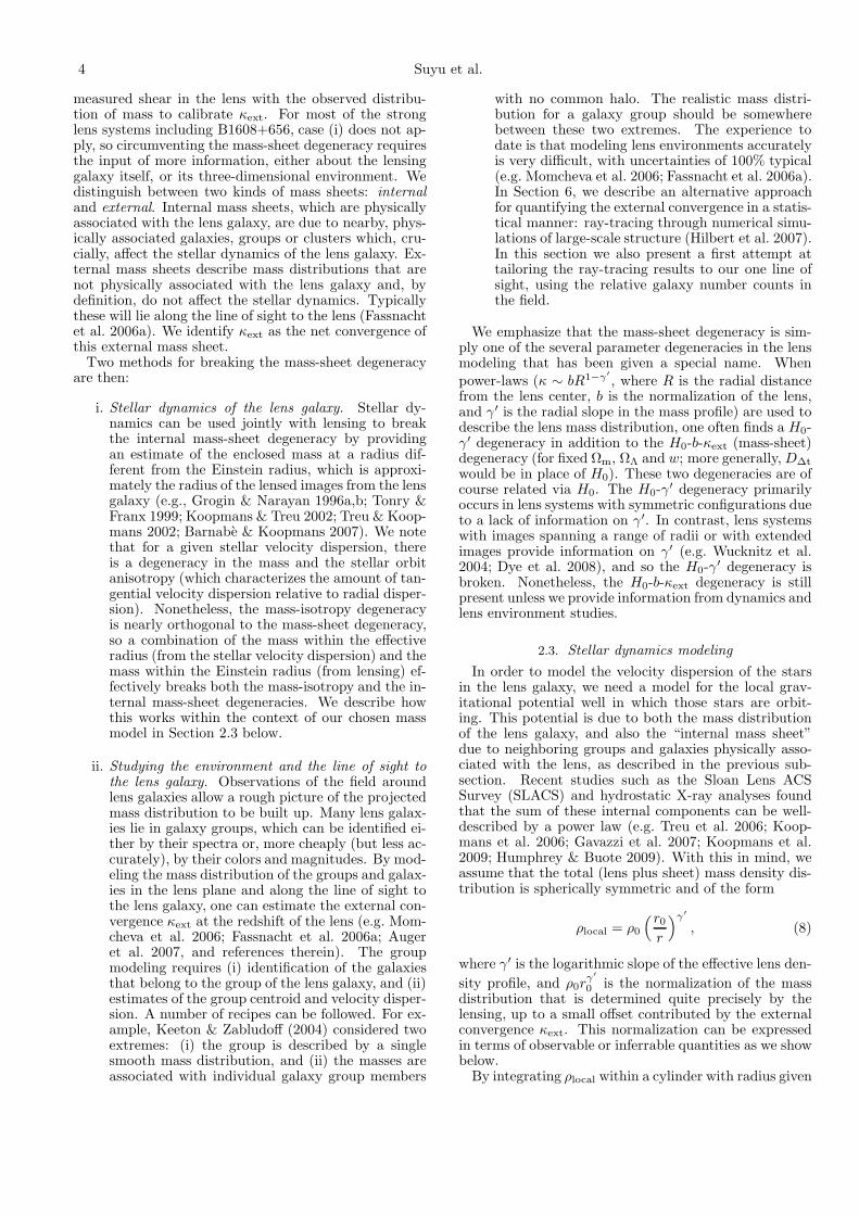
The quadruple-image gravitational lens B1608+656was discovered in the Cosmic Lens All-Sky Survey(CLASS) (Myers et al. 1995; Browne et al. 2003; My-ers et al. 2003). Figure 1 is an image of B1608+656,showing the spatially extended source surface brightnessdistribution (with lensed images labeled by A, B, C, andD) and two interacting galaxy lenses (labeled by G1 andG2). The redshifts of the source and the lens galaxies

8 Suyu et al.

DG1

C

A

B

G2

1"

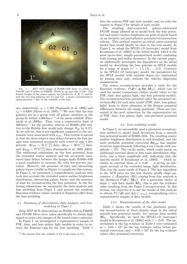
Fig. 1.— HST ACS image of B1608+656 from 11 orbits inF814W and 9 orbits in F606W. North is up and east is left. Thelensed images of the source galaxy are labeled by A, B, C, and D,and the two lens galaxies are G1 and G2. 1 arcsec corresponds toapproximately 7 kpc at the redshift of the lens.

are, respectively, zs = 1.394 (Fassnacht et al. 1996) andzd = 0.6304 (Myers et al. 1995).11 We note that the lensgalaxies are in a group with all galaxy members in thegroup lie within ±300 km s−1 of the mean redshift (Fass-nacht et al. 2006a). Thus, even a conservative limit of300 km s−1 for the peculiar velocity of B1608+656 rela-tive to the Hubble flow would only change D∆t by 0.5%.As we will see, this is not significant compared to the sys-tematic error associated with κext. This system is specialin that the three relative time delays between the four im-ages were measured accurately with errors of only a fewpercent: ∆tAB = 31.5+2.0

−1.0 days, ∆tCB = 36.0+1.5−1.5 days,

and ∆tDB = 77.0+2.0−1.0 days (Fassnacht et al. 1999, 2002).

The additional constraints on the lens potential fromthe extended source analysis and the accurately mea-sured time delays between the images make B1608+656a good candidate to measure H0 with few-percent pre-cision. However, the presence of dust and interactinggalaxy lenses (visible in Figure 1) complicate this system.In Paper I, we presented a comprehensive analysis thattook into account the extended source surface brightnessdistribution, interacting galaxy lenses, and the presenceof dust for reconstructing the lens potential. In the fol-lowing subsections, we summarize the data analysis andlens modeling from Paper I, and present the resultingBayesian evidence values (needed in Equation (30)) fromthe lens modeling.

4.1. Summary of observations, data analysis, and lensmodeling in Paper I

Deep HST ACS observations on B1608+656 in F606Wand F814W filters were taken specifically to obtain highsignal-to-noise ratio images of the lensed source emission.

In Paper I, we investigated a representative sample ofPSF, dust, and lens galaxy light models in order to ex-tract the Einstein ring for the lens modeling. Table 1

11 We assume that the redshift of G2 is the same as G1.

lists the various PSF and dust models, and we refer thereaders to Paper I for details of each model.

The resulting dust-corrected, galaxy-subtractedF814W image allowed us to model both the lens poten-tial and source surface brightness on grids of pixels basedon an iterative and perturbative potential reconstructionscheme. This method requires an initial guess potentialmodel that would ideally be close to the true model. InPaper I, we adopt the SPLE1+D (isotropic) model fromKoopmans et al. (2003) as the initial model, which is themost up-to-date, simply-parametrized model combiningboth lensing and stellar dynamics. In the current paper,we additionally investigate the dependence on the initialmodel by describing the lens galaxies as SPLE modelsfor a range of slopes (γ′ = 1.5, 1.6, . . . , 2.5). Contraryto the SPLE1+D (isotropic) model, the parameters forthe SPLE models with variable slopes are constrainedby lensing data only, without the velocity dispersionmeasurement.

The source reconstruction provides a value for theBayesian evidence, P (d|γ′,η, δψ,MD), which can beused for model comparison (where model refers to thePSF, dust, lens galaxy light, and lens potential model).The reconstructed lens potential (after the pixelated cor-rections δψ) for each data model (PSF, dust, lens galaxylight) leads to three estimates of the Fermat potentialdifferences between the image positions. These are pre-sented in the next subsection for the representative setof PSF, dust, lens galaxy light, and pixelated potentialmodel.

4.2. Lens modeling results

In Paper I, we successfully used a pixelated reconstruc-tion method to model small deviations from a smoothlens potential model of B1608+656. The resulting sourcesurface brightness distribution is well-localized, and themost probable potential correction δψMP has angularstructure approximately following a cosφ mode with am-plitude ∼ 2%. The cos 2φ mode, which could mimic anadditional external shear or lens mass distribution ellip-ticity, has a lower amplitude still, indicating that thesmooth model of Koopmans et al. (2003) — which in-cludes an external shear of ' 0.08 — is giving an ade-quate account of the extended image light distribution.This was the main result of Paper I. The key ingredientin the ACS prior for the lens density profile slope pa-rameter γ′ (Equation (30)) coming from this analysis isthe likelihood P (d|γ′,MD). For a particular choice ofslope γ′ and data model MD, this is just the evidencevalue resulting from the Paper I reconstruction. In thissection, our objective is to use the results of this analysisto obtain P (γ′|d) and ∆φ(γ′, κext), marginalizing over arepresentative sample of data models.

4.2.1. Marginalization of the data model

Table 1 shows the results of the pixelated poten-tial reconstruction at fixed density slope in the initialsmooth lens potential model, for various data modelsMD. Specifically, we used the SPLE1+D (isotropic)model in Koopmans et al. (2003) with γ′ = 2.05. The un-certainties in the log evidence in Table 1 were estimatedas ∼ 0.03 × 104 for the log evidence values before po-tential correction, and ∼ 0.05 × 104 for the log evidencevalues after potential correction.

Cosmological constraints from gravitational lens B1608+656 9

We see a clear division between models with high andlow evidence values, the two groups being separated bya very large factor in probability. Assuming that all thedata models MD are equally probable a priori, the con-tribution to the marginalized distribution P (π|∆t,d, σ)(Equation (24)) from these lower-evidence models will benegligible.

The physical difference between these evidence-rankeddata models is in the dust correction: the 2-band dustmodels are found to be less probable than the 3-banddust models. It is useful to quantify the systematic errorthat would occur with the use of 2-band dust models(which was avoided from the evidence ranking) in termsof the H0 value implied by the system. For this simpleerror estimation we use Equation (5) and assert Ωm =0.3, ΩΛ = 0.7, w = −1 and zero external convergence,as a fiducial reference cosmology (Koopmans et al. 2003).The implied Hubble constants are shown in the final fourcolumns of Table 1. We see that the disfavored use of the2-band dust maps would have led to values of H0 some15% lower than that inferred from the 3-band maps.

We note that the evidence values of each of the 3-banddust map models MD are the same within their uncer-tainties. We can also see that for good data models,specifically MD = M5, the three H0 values have lowscatter: these lens models are internally self-consistent.Furthermore, the scatter between the values for the dif-ferent good data models is also low: the high evidencedata models consistently return the same Hubble con-stant. This is the basis for the approximations (in Sec-tion 3.3 and Appendix A) that the likelihood P (∆t|ξ)is effectively constant with the 3-band dust map mod-els MD. Assuming that we have indeed obtained theoptimal set of MD, we can approximate the likelihoodsin Equations (30) and (33) as being evaluated for modelM5.

4.2.2. Effects of the potential corrections

Having approximately marginalized out MD by con-ditioning on M5, we now consider the impact of the po-tential corrections discussed in Paper I. In particular, weseek the likelihood for the density profile slope parame-ter γ′, P (d|γ′ = γ′i,η, δψMP,MD = M5). We charac-terize this function on a grid of slope values in the rangeof γ′ = 1.5, 1.6 . . . , 2.5, first re-optimizing the parame-ters of the smooth lens model, and then computing thesource reconstruction evidences both with and withoutpotential correction. These are tabulated in Table 2. Weagain compute the Fermat potential differences and im-plied Hubble constant values as before.

The spread of the three implied H0 values at fixed den-sity slope is again small: we conclude that the internalself-consistency of the lens model depends on the datamodel but not γ′. The table also shows that the smoothSPLE model provides a good estimate of the relative Fer-mat potentials. Indeed, this was the principal conclusionof Paper I. The relative thickness of the arcs is sensitiveto the SPLE density profile slope γ′, as can be seen inthe first two columns of Table 2: the evidence clearly fa-vors γ′ ' 2.05, as previously found by Koopmans et al.(2003). Indeed, exponentiating this gives quite a sharplypeaked function, which we return to below.

How is the potential correction then affecting themodel? In Table 2 we can see that the corrected poten-

tial leads to nearly the same evidence value (P (d|γ′ =γ′i,η, δψMP,MD = M 5)) for a wide range of underly-ing density slopes, and yet barely changes the relativeFermat potential values. The unchanging nature of theFermat potential is due to the curvature type of regu-larization on the potential corrections suppressing theaddition of mass within the potential reconstruction an-nulus. From Kochanek (2002), the relative Fermat po-tential depends only on the mean surface mass densityenclosed in the annulus between the images, to first or-der in δR/〈R〉, where δR is the difference in the radialdistance of the image locations from the effective cen-ter of the lens galaxies and 〈R〉 is the mean radius ofthe images. The mean surface mass density depends onthe slope of the initial SPLE model (hence the trendwe see in relative Fermat potential in the left-hand sideof Table 2), but not on the potential corrections due tothe curvature regularization imposed. Therefore, to firstorder in δR/〈R〉, the Fermat potential depends only in-directly on γ′ via the mean surface mass density. Thesecond order term is very small — it has a prefactor of1/12 and for B1608+656, (δR/〈R〉)2 ∼ 0.1. Therefore,for good and self-consistent data models, the potentialcorrections δψMP do not change the Fermat potentialsignificantly.

The right-hand side of Table 2, where a wide range ofinitial slope values provide good fits to the data, is there-fore effectively a manifestation of the mass-sheet degen-eracy. One can understand the effect of the potentialcorrections as making local corrections to the effectivedensity profile slope in order to fit the ACS data. Thechange in slope by the pixelated corrections would cre-ate a deficit/surplus of mass in the annulus, which thepixelated potential corrections then add/subtract backinto the annulus in the form of a constant mass sheetto (i) enforce the prior (no net addition of mass withinannulus) and (ii) continue to fit the arcs equally well.

We conclude that the value of the potential correc-tion analysis is in demonstrating that the double SPLEmodel for B1608+656 is, despite the system’s complex-ity, a good model for the high fidelity HST data. Thecorrections are small in magnitude (' 2% relative to theinitial SPLE model), and the inclusion of the δψ nei-ther significantly reduces the dispersion in implied H0

values between the image pairs, nor alters the rank orderof the data models. We therefore use the informationon the slope of the initial SPLE model from the ACSdata without potential corrections, thus using the infor-mation on the relative thickness of the lensed extendedimages clearly present. How we derive our estimate forP (d|γ′,MD) from column 2 of Table 2 is described next.

4.2.3. The ACS posterior PDF for γ′

In the previous section, we explored the HST data con-straints on the slope parameter, optimizing the otherparameters of the SPLE lens model at each step. Tocharacterize properly P (γ′|d,MD = M5) in Equation(30), we would need to marginalize over all lens param-eters η instead. However, as we shall now see, this opti-mization approximation is actually a good one and iscertainly the most tractable solution due to the highdimensionality of the problem (16 parameters to de-scribe G1, G2 and external shear). Direct sampling inthe 16-dimensional parameter space of P (d|γ′,η,MD =

10 Suyu et al.

TABLE 1log evidence values and relative Fermat potential values before and after the pixelated potential reconstruction for

various data models with the SPLE1+D (isotropic) initial model

Data Model Initial Potential Corrected Potential

Model PSF dust log P log P ∆φAB ∆φCB ∆φDB HAB0 HCB

0 HDB0 H0

(×104) (×104)

5 B1 3-band 1.56 1.77 0.244 0.279 0.575 78.1 78.1 75.1 77.1 ± 1.79 C B1/3-band 1.56 1.76 0.240 0.280 0.563 76.7 78.3 73.5 76.2 ± 2.43 C 3-band 1.60 1.76 0.243 0.277 0.570 77.6 77.5 74.4 76.5 ± 1.82 drz 3-band 1.48 1.75 0.238 0.278 0.548 76.0 77.7 71.6 75.1 ± 3.17 B2 3-band 1.55 1.75 0.237 0.274 0.571 75.7 76.7 74.6 75.7 ± 1.0

11 B1 no dust 1.27 1.72 0.229 0.263 0.576 73.2 73.6 75.3 74.0 ± 1.110 B1 C/2-band 1.36 1.61 0.193 0.227 0.565 61.8 63.5 73.8 66.4 ± 6.44 C 2-band 1.40 1.58 0.199 0.234 0.560 63.6 65.6 73.1 67.4 ± 5.06 B1 2-band 1.10 1.41 0.196 0.226 0.559 62.5 63.2 73.0 66.2 ± 5.88 B2 2-band 1.23 1.40 0.201 0.234 0.556 64.3 65.4 72.7 67.4 ± 4.5

∆φ and H0 values from initial SPLE1+D (isotropic)

0.243 0.271 0.575 77.7 75.8 75.1 76.2 ± 1.3

Notes — The uncertainties in the log evidence before and after the potential corrections are ∼ 0.03 × 104 and ∼ 0.05 × 104, respectively.The relative Fermat potentials are in units of arcsec2, and the H0 values are in units of km s−1 Mpc−1. The H0 values are the mean andstandard deviation from the mean of the three estimates obtained using the initial/corrected potential and the three time delays, withouttaking into account the uncertainties associated with the time delays. These H0 values assume Ωm = 0.3, ΩΛ = 0.7 and w = −1, andare listed purely to aid the digestion of the ∆φ values. The full analysis for obtaining the probability distribution for the cosmologicalparameters is described in Section 8.

TABLE 2log evidence value before and after the pixelated potential reconstruction for initial models with various slope using

PSF-B1 and the 3-band dust map (MD=Model 5)

Initial Potential Corrected Potential

γ′ log P ∆φAB ∆φCB ∆φDB HAB0 HCB

0 HDB0 H0 log P ∆φAB ∆φCB ∆φDB HAB

0 HCB0 HDB

0 H0

(×104) (×104)

1.5 1.38 0.125 0.139 0.287 40.2 39.0 37.6 38.9 ± 1.3 1.73 0.130 0.143 0.290 41.7 40.2 38.0 39.9 ± 1.91.6 1.48 0.147 0.163 0.338 47.2 45.8 44.3 45.7 ± 1.4 1.77 0.150 0.170 0.349 48.1 47.6 45.6 47.1 ± 1.31.7 1.52 0.174 0.193 0.403 55.5 54.0 52.7 54.0 ± 1.4 1.75 0.178 0.201 0.417 57.0 56.2 54.5 55.9 ± 1.31.8 1.54 0.190 0.211 0.442 60.8 59.1 57.7 59.2 ± 1.5 1.77 0.194 0.215 0.457 61.9 60.2 59.7 60.7 ± 1.21.9 1.58 0.210 0.234 0.491 67.1 65.4 64.1 65.6 ± 1.4 1.76 0.210 0.237 0.510 67.3 66.4 66.6 66.8 ± 0.52.0 1.60 0.229 0.256 0.540 73.3 71.6 70.5 71.8 ± 1.3 1.79 0.231 0.261 0.549 73.8 73.0 71.7 72.9 ± 1.12.1 1.60 0.247 0.276 0.586 79.0 77.3 76.6 77.6 ± 1.2 1.79 0.250 0.287 0.606 80.0 80.1 79.1 79.8 ± 0.52.2 1.58 0.264 0.296 0.632 84.5 82.8 82.6 83.3 ± 1.0 1.77 0.258 0.299 0.648 82.5 83.7 84.6 83.7 ± 1.12.3 1.57 0.281 0.315 0.676 89.8 88.0 88.3 88.7 ± 0.9 1.79 0.267 0.311 0.678 85.3 86.9 88.5 86.9 ± 1.62.4 1.55 0.297 0.332 0.720 94.8 92.8 94.0 93.9 ± 1.0 1.79 0.299 0.344 0.738 95.6 96.3 96.4 96.2 ± 0.42.5 1.49 0.312 0.348 0.763 99.8 97.4 99.6 98.9 ± 1.3 1.78 0.311 0.357 0.759 99.4 99.7 99.1 99.5 ± 0.3

Notes — notation and uncertainties are the same as those described in the notes for Table 1.

M5)Pno ACS(γ′)P (η) in Equation (30) via, for example,Markov chain Monte Carlo (MCMC) techniques usingthe extended source information is not feasible on a rea-sonable time scale. Importance sampling of the priorPDF from the radio data of image positions and fluxes(Pno ACS(γ′,η) = PnoACS(γ′,η|radio)) by weighing thesamples by P (d|γ′,η,MD = M 5) is difficult since γ′

is effectively unconstrained by the radio data (the χ2

changes by . 1 in the slope range between 1.5 and 2.5).12

It is precisely the unconstrained nature of the γ′ pa-rameter that makes the optimization approximation sogood. The “tube” of γ′-degeneracy traversing the 16-dimensional parameter space dominates the uncertaintiesin the parameters. We thus assume that the tube of γ′-degeneracy has negligible thickness (a degeneracy curve),and use P (d|γ′,η,MD = M5) to break the degeneracy.Specifically, we use the radio observations, HST Near In-frared Camera and Multi-Object Spectrometer 1 (NIC-

12 We set γ′

G2 = γ′

G1 = γ′ since the slope of G2 is ill-constrained(Koopmans et al. 2003).

MOS) images (Proposal 7422; PI:Readhead), and timedelay data to obtain the best-fitting η for a given γ′=γ′i(assuming Ωm = 0.3, ΩΛ = 0.7 and w = −1 in usingthe time delay data), and compute the correspondingP (d|γ′i, η,MD = M5). These are the listed evidencevalues in the second column of Table 2 for the various γ′ivalues. The time delay data are included because the pre-dicted relative Fermat potential among the image pairsusing the radio and NICMOS data are otherwise incon-sistent with one another. The optimized parameters fromonly the radio and NICMOS data lead to χ2 ∼ 600 forjust the time delay data; including the time delay datareduces the time delay χ2 to ∼ 1 with only a mild in-crease in the radio and NICMOS χ2 of ∼ 6. We “undo”the inclusion of the time delay data (so that we do notuse the time delay data twice in the importance sam-pling of Equation (33)) by subtracting the log likelihoodof the time delay from the log likelihood of d; the effect isnegligible since the latter is ∼ 104 higher in magnitude.

Our thin degeneracy tube assumption implies that

Cosmological constraints from gravitational lens B1608+656 11

P (d|γ′) ' P (d|γ′, η), such that the posterior PDF forthe slope is P (γ′|d) ∝ P (d|γ′) PnoACS(γ′). Assigning auniform prior (i.e., PnoACS(γ′) is constant), we arrive atthe result that our desired PDF is just the exponentia-tion of the log evidence in column 2 of Table 2. Fittingthese log evidences with the following quadratic function,

logP (γ′|d) = C − (γ′ − γ′0)2

2σ2γ′

, (34)

we obtain the following best-fit parameter values: γ′0 =2.081 ± 0.027, σγ′ = 0.0091 ± 0.0008, and C = (1.60 ±0.01) × 104. While the PDF width σγ′ is very small,the centroid is not well determined. Adding σγ′ and theuncertainty in γ′0 in quadrature, we finally approximateP (γ′|d) with a Gaussian centered on 2.08 with standarddeviation 0.03. This provides the prior on γ′ from theACS data (in Equation (33)).

The deep ACS data therefore allow a significant im-provement to the previous measurement in Koopmanset al. (2003) of γ′ = 1.99± 0.20, which was based on theradio data and the NICMOS ring. Coincidentally, ourγ′ = 2.08 ± 0.03 is identical, apart from the spread, tothe measurement from SLACS of γ′ = 2.08±0.2 that wasbased on a sample of massive elliptical lenses (Koopmanset al. 2009). The spread of 0.2 in the SLACS measure-ment is the intrinsic scatter of slope values in the sam-ple, and is larger than the typical uncertainties associatedwith individual systems in the sample of ∼ 0.15. We notethat our measurement is not the first percent-level deter-mination of a strong lens density profile slope. Wucknitzet al. (2004) used high precision astrometric measure-ments from VLBI data to constrain the γ′ parameter inB0218+357 to be 1.96±0.02 (where we have transformedtheir β into our notation). However, they did not use ex-actly the same model as we do here (instead workingwith combinations of isothermal elliptical potentials andneglecting external convergence). Dye & Warren (2005)measured the power-law slope of the lens galaxy in theEinstein ring system 0047-2808 to be γ′ = 2.11 ± 0.04based on the extended image constraints. More recently,Dye et al. (2008) determined the power-law slope of theextremely massive and luminous lens galaxy in the Cos-mic Horseshoe Einstein ring system J1004+4112 to beγ′ = 1.96 ± 0.02.

4.2.4. Predicted relative Fermat potentials

In order to be able to calculate the time delay like-lihood function, P (∆t|zd, zs,π, γ′, κext,MD), at anyvalue of the slope γ′, we need to interpolate the Fermatpotential differences given in Table 2. In fact, these datagive us the function q(γ′) to insert into Equation (25):we can do the interpolation at κext = 0.0 and then rescaleby (1 − κext) without loss of generality.

For each of the image pairs, we fit the relative Fermatpotential difference as a third-order polynomial functionof γ′ using the values we have at the discrete pointsγ′i for the SPLE models in the table. Recall that theSPLE model provides an unbiased estimate of the rel-ative Fermat potential, and that the various top datamodels MD gave consistent estimates. Thus, the poly-nomial fit gives the function q(γ′,MD) in Equation(25). The third-order polynomial fit leads to residuals(= (∆φi −∆φpoly)/(∆φi)) of < 1% for all image pairs at

all slope points in Table 2 except for γ′i = 1.7, which hasresiduals of ∼ 2%.

5. BREAKING THE MASS-SHEET DEGENERACY:STELLAR DYNAMICS

In this section, we present the observations and datareduction for measuring the velocity dispersion σ of G1 inB1608+656. This measurement appears as the likelihoodfunction given in Equation (32) above.

5.1. Observations

We have obtained a high signal-to-noise spectrumof B1608+656 using the Low-Resolution Imaging Spec-trometer (LRIS; Oke et al. 1995) on Keck 1. The datawere obtained from the red side of the spectrograph on12 June 2007 using the 831/8200 grating with the D680dichroic in place. A slit mask was employed to obtainsimultaneously spectra for two additional strong lensesin the field (Fassnacht et al. 2006b) and to continue toprobe the structure along the line of sight to the lens(Fassnacht et al. 2006a). The night was clear with anominal seeing of 0.′′9, and 10 exposures of 1800s andone exposure of 600s were obtained for a total exposuretime of 18600s.

Each exposure was reduced individually using a custompipeline (see Auger et al. 2008, for details) that performsa single resampling of the spectra onto a constant wave-length grid; the same wavelength grid was used for allexposures to avoid resampling the spectra when combin-ing them, and an output pixel scale of 0.915 A was usedto match the dispersion of the 831/8200 grating. Individ-ual spectra were extracted from an aperture 0.′′84 wide(corresponding to 4 pixels on the LRIS red side) centeredon the peak of the flux of the lensing galaxy G1. The sizeof the aperture was chosen to avoid contamination fromthe spectrum of G2 while maximizing the total flux foran improved signal-to-noise ratio. The extracted spectrawere combined by clipping the extreme points at eachwavelength and taking the variance-weighted sum of theremaining data points. The same extraction and coad-dition scheme was performed for a sky aperture to de-termine the resolution of the output co-added spectrum;we find the resolution to be R = 2560, corresponding toσobs = 49.7 km s−1. The signal-to-noise ratio per pixel ofthe final spectrum is ∼ 60.

5.2. Velocity dispersion measurement

We use a Python-based implementation of the velocity-dispersion code from van der Marel (1994), with one im-portant modification. Our implementation allows for alinear sum of template spectra to be modeled using abounded variable least squares solver with the constraintthat each template must have a non-negative coefficient.We use a set of templates from the INDO-US stellar li-brary containing spectra for a set of seven K and G gi-ants with a variety of temperatures and spectra for anF2 and an A0 giant. These templates of early-type starsare particularly important for B1608+656, which has apost-starburst spectrum (Myers et al. 1995).

We perform our modeling over a wide range of wave-length intervals and find a stable solution over a va-riety of spectral features; we therefore choose to usethe rest-frame range from 4200 A to 4900 A for ourfit. The INDO-US templates have a constant-wavelength

12 Suyu et al.

!"# !$%

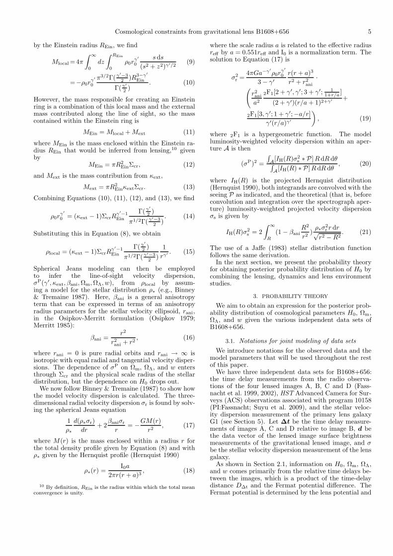
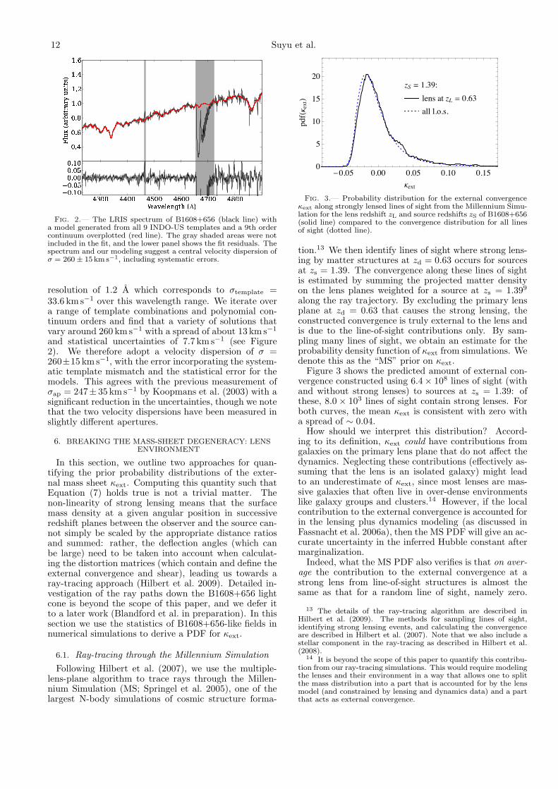
Fig. 2.— The LRIS spectrum of B1608+656 (black line) witha model generated from all 9 INDO-US templates and a 9th ordercontinuum overplotted (red line). The gray shaded areas were notincluded in the fit, and the lower panel shows the fit residuals. Thespectrum and our modeling suggest a central velocity dispersion ofσ = 260 ± 15 km s−1, including systematic errors.

resolution of 1.2 A which corresponds to σtemplate =33.6 km s−1 over this wavelength range. We iterate overa range of template combinations and polynomial con-tinuum orders and find that a variety of solutions thatvary around 260 km s−1 with a spread of about 13 km s−1

and statistical uncertainties of 7.7 km s−1 (see Figure2). We therefore adopt a velocity dispersion of σ =260±15 km s−1, with the error incorporating the system-atic template mismatch and the statistical error for themodels. This agrees with the previous measurement ofσap = 247± 35 km s−1 by Koopmans et al. (2003) with asignificant reduction in the uncertainties, though we notethat the two velocity dispersions have been measured inslightly different apertures.

6. BREAKING THE MASS-SHEET DEGENERACY: LENSENVIRONMENT

In this section, we outline two approaches for quan-tifying the prior probability distributions of the exter-nal mass sheet κext. Computing this quantity such thatEquation (7) holds true is not a trivial matter. Thenon-linearity of strong lensing means that the surfacemass density at a given angular position in successiveredshift planes between the observer and the source can-not simply be scaled by the appropriate distance ratiosand summed: rather, the deflection angles (which canbe large) need to be taken into account when calculat-ing the distortion matrices (which contain and define theexternal convergence and shear), leading us towards aray-tracing approach (Hilbert et al. 2009). Detailed in-vestigation of the ray paths down the B1608+656 lightcone is beyond the scope of this paper, and we defer itto a later work (Blandford et al. in preparation). In thissection we use the statistics of B1608+656-like fields innumerical simulations to derive a PDF for κext.

6.1. Ray-tracing through the Millennium Simulation

Following Hilbert et al. (2007), we use the multiple-lens-plane algorithm to trace rays through the Millen-nium Simulation (MS; Springel et al. 2005), one of thelargest N-body simulations of cosmic structure forma-

zS ! 1.39:

lens at zL ! 0.63

all l.o.s.

"0.05 0.00 0.05 0.10 0.150

5

10

15

20

Κext

pdf!Κext"

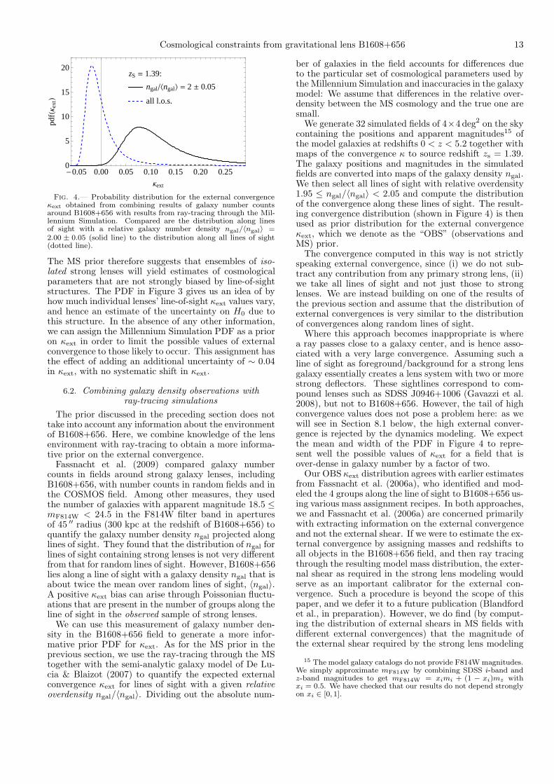
Fig. 3.— Probability distribution for the external convergenceκext along strongly lensed lines of sight from the Millennium Simu-lation for the lens redshift zL and source redshifts zS of B1608+656(solid line) compared to the convergence distribution for all linesof sight (dotted line).

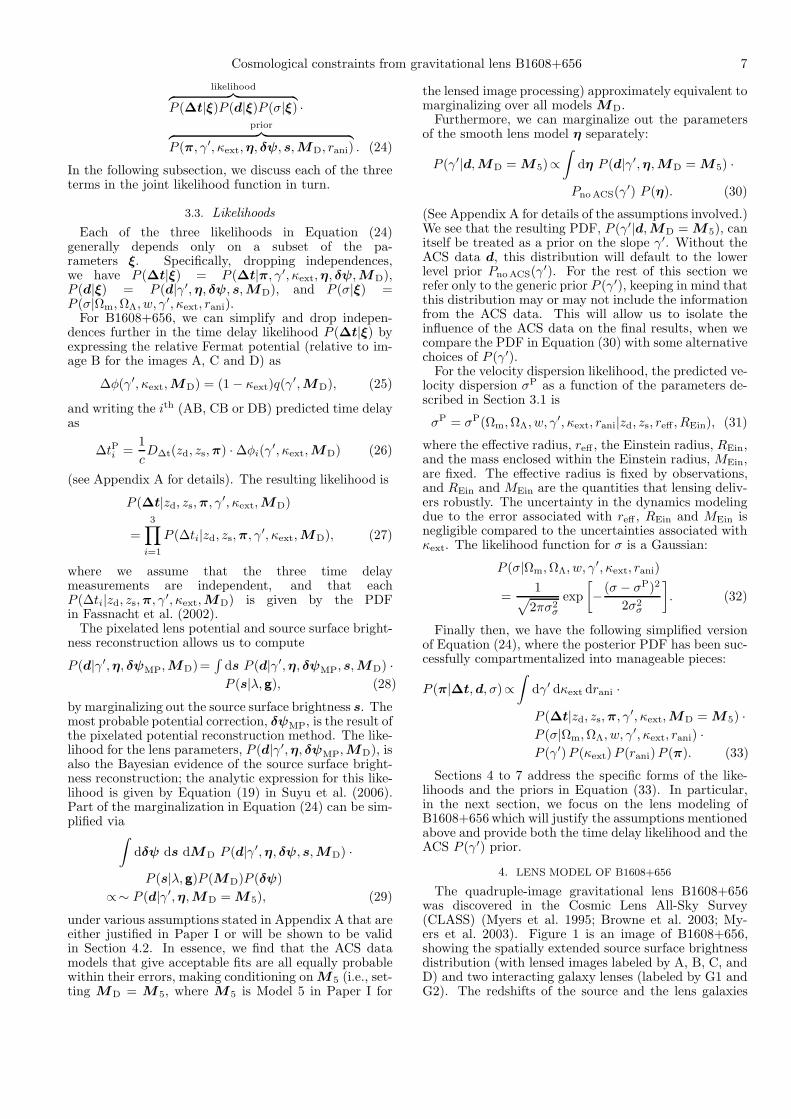
tion.13 We then identify lines of sight where strong lens-ing by matter structures at zd = 0.63 occurs for sourcesat zs = 1.39. The convergence along these lines of sightis estimated by summing the projected matter densityon the lens planes weighted for a source at zs = 1.399

along the ray trajectory. By excluding the primary lensplane at zd = 0.63 that causes the strong lensing, theconstructed convergence is truly external to the lens andis due to the line-of-sight contributions only. By sam-pling many lines of sight, we obtain an estimate for theprobability density function of κext from simulations. Wedenote this as the “MS” prior on κext.

Figure 3 shows the predicted amount of external con-vergence constructed using 6.4 × 108 lines of sight (withand without strong lenses) to sources at zs = 1.39: ofthese, 8.0 × 103 lines of sight contain strong lenses. Forboth curves, the mean κext is consistent with zero witha spread of ∼ 0.04.

How should we interpret this distribution? Accord-ing to its definition, κext could have contributions fromgalaxies on the primary lens plane that do not affect thedynamics. Neglecting these contributions (effectively as-suming that the lens is an isolated galaxy) might leadto an underestimate of κext, since most lenses are mas-sive galaxies that often live in over-dense environmentslike galaxy groups and clusters.14 However, if the localcontribution to the external convergence is accounted forin the lensing plus dynamics modeling (as discussed inFassnacht et al. 2006a), then the MS PDF will give an ac-curate uncertainty in the inferred Hubble constant aftermarginalization.

Indeed, what the MS PDF also verifies is that on aver-age the contribution to the external convergence at astrong lens from line-of-sight structures is almost thesame as that for a random line of sight, namely zero.

13 The details of the ray-tracing algorithm are described inHilbert et al. (2009). The methods for sampling lines of sight,identifying strong lensing events, and calculating the convergenceare described in Hilbert et al. (2007). Note that we also include astellar component in the ray-tracing as described in Hilbert et al.(2008).

14 It is beyond the scope of this paper to quantify this contribu-tion from our ray-tracing simulations. This would require modelingthe lenses and their environment in a way that allows one to splitthe mass distribution into a part that is accounted for by the lensmodel (and constrained by lensing and dynamics data) and a partthat acts as external convergence.

Cosmological constraints from gravitational lens B1608+656 13

zS = 1.39:

ngalXngal\ = 2 ± 0.05

all l.o.s.

-0.05 0.00 0.05 0.10 0.15 0.20 0.250

5

10

15

20

Κext

pdfHΚ

extL

Fig. 4.— Probability distribution for the external convergenceκext obtained from combining results of galaxy number countsaround B1608+656 with results from ray-tracing through the Mil-lennium Simulation. Compared are the distribution along linesof sight with a relative galaxy number density ngal/〈ngal〉 =2.00 ± 0.05 (solid line) to the distribution along all lines of sight(dotted line).

The MS prior therefore suggests that ensembles of iso-lated strong lenses will yield estimates of cosmologicalparameters that are not strongly biased by line-of-sightstructures. The PDF in Figure 3 gives us an idea of byhow much individual lenses’ line-of-sight κext values vary,and hence an estimate of the uncertainty on H0 due tothis structure. In the absence of any other information,we can assign the Millennium Simulation PDF as a prioron κext in order to limit the possible values of externalconvergence to those likely to occur. This assignment hasthe effect of adding an additional uncertainty of ∼ 0.04in κext, with no systematic shift in κext.

6.2. Combining galaxy density observations withray-tracing simulations

The prior discussed in the preceding section does nottake into account any information about the environmentof B1608+656. Here, we combine knowledge of the lensenvironment with ray-tracing to obtain a more informa-tive prior on the external convergence.

Fassnacht et al. (2009) compared galaxy numbercounts in fields around strong galaxy lenses, includingB1608+656, with number counts in random fields and inthe COSMOS field. Among other measures, they usedthe number of galaxies with apparent magnitude 18.5 ≤mF814W < 24.5 in the F814W filter band in aperturesof 45 ′′ radius (300 kpc at the redshift of B1608+656) toquantify the galaxy number density ngal projected alonglines of sight. They found that the distribution of ngal forlines of sight containing strong lenses is not very differentfrom that for random lines of sight. However, B1608+656lies along a line of sight with a galaxy density ngal that isabout twice the mean over random lines of sight, 〈ngal〉.A positive κext bias can arise through Poissonian fluctu-ations that are present in the number of groups along theline of sight in the observed sample of strong lenses.

We can use this measurement of galaxy number den-sity in the B1608+656 field to generate a more infor-mative prior PDF for κext. As for the MS prior in theprevious section, we use the ray-tracing through the MStogether with the semi-analytic galaxy model of De Lu-cia & Blaizot (2007) to quantify the expected externalconvergence κext for lines of sight with a given relativeoverdensity ngal/〈ngal〉. Dividing out the absolute num-

ber of galaxies in the field accounts for differences dueto the particular set of cosmological parameters used bythe Millennium Simulation and inaccuracies in the galaxymodel: We assume that differences in the relative over-density between the MS cosmology and the true one aresmall.

We generate 32 simulated fields of 4×4 deg2 on the skycontaining the positions and apparent magnitudes15 ofthe model galaxies at redshifts 0 < z < 5.2 together withmaps of the convergence κ to source redshift zs = 1.39.The galaxy positions and magnitudes in the simulatedfields are converted into maps of the galaxy density ngal.We then select all lines of sight with relative overdensity1.95 ≤ ngal/〈ngal〉 < 2.05 and compute the distributionof the convergence along these lines of sight. The result-ing convergence distribution (shown in Figure 4) is thenused as prior distribution for the external convergenceκext, which we denote as the “OBS” (observations andMS) prior.

The convergence computed in this way is not strictlyspeaking external convergence, since (i) we do not sub-tract any contribution from any primary strong lens, (ii)we take all lines of sight and not just those to stronglenses. We are instead building on one of the results ofthe previous section and assume that the distribution ofexternal convergences is very similar to the distributionof convergences along random lines of sight.

Where this approach becomes inappropriate is wherea ray passes close to a galaxy center, and is hence asso-ciated with a very large convergence. Assuming such aline of sight as foreground/background for a strong lensgalaxy essentially creates a lens system with two or morestrong deflectors. These sightlines correspond to com-pound lenses such as SDSS J0946+1006 (Gavazzi et al.2008), but not to B1608+656. However, the tail of highconvergence values does not pose a problem here: as wewill see in Section 8.1 below, the high external conver-gence is rejected by the dynamics modeling. We expectthe mean and width of the PDF in Figure 4 to repre-sent well the possible values of κext for a field that isover-dense in galaxy number by a factor of two.

Our OBS κext distribution agrees with earlier estimatesfrom Fassnacht et al. (2006a), who identified and mod-eled the 4 groups along the line of sight to B1608+656 us-ing various mass assignment recipes. In both approaches,we and Fassnacht et al. (2006a) are concerned primarilywith extracting information on the external convergenceand not the external shear. If we were to estimate the ex-ternal convergence by assigning masses and redshifts toall objects in the B1608+656 field, and then ray tracingthrough the resulting model mass distribution, the exter-nal shear as required in the strong lens modeling wouldserve as an important calibrator for the external con-vergence. Such a procedure is beyond the scope of thispaper, and we defer it to a future publication (Blandfordet al., in preparation). However, we do find (by comput-ing the distribution of external shears in MS fields withdifferent external convergences) that the magnitude ofthe external shear required by the strong lens modeling

15 The model galaxy catalogs do not provide F814W magnitudes.We simply approximate mF814W by combining SDSS i-band andz-band magnitudes to get mF814W = ximi + (1 − xi)mz withxi = 0.5. We have checked that our results do not depend stronglyon xi ∈ [0, 1].

14 Suyu et al.

(γext ' 0.075) is consistent with the external shear am-plitude predicted in the OBS scenario for the B1608+656field.

6.3. The influence on lens modeling.

As already remarked, the description of ray propaga-tion in an inhomogeneous cosmology is quite subtle. Thematter (dark plus baryonic) density is partitioned be-tween virialized structures (galaxies, groups and clusters)and a depleted background medium. Any structures suf-ficiently close to the line of sight will imprint convergenceand shear onto a ray congruence. Meanwhile the back-ground medium will contribute less Ricci focusing thanwould be present in a homogeneous, flat universe andwill diminish the net convergence.

As the foregoing discussion makes clear, the line ofsight to B1608+656 is unusual and we know quite a lotabout the photometry and redshifts of the interveninggalaxies. It is therefore possible, in principle, to makea refined estimate of the external convergence and shearand to compare the former with the simulations discussedabove and the latter with the shear inferred in the lensmodel described in Paper I. In this way, the shear, againin principle, can be used to calibrate κext.

There is a second complication that must be addressed.Matter inhomogeneities in front of G1 and G2 distort theimage of the primary lens as well as the multiple imagesof the source. Inhomogeneities behind the lens contributefurther distortion in the images of the source. In a moreaccurate approach, these effects should be taken into ac-count explicitly in the construction of the lens model,while here we are subsuming them in a single correctionfactor κext. The way that the resulting corrections af-fect the inference of a value for H0 turns out to be quitecomplex. However, it appears that in the particular caseof B1608+656, the error that is incurred does not con-tribute significantly to our quoted errors.

These matters will be discussed in a forthcoming pub-lication.

7. PRIORS FOR MODEL PARAMETERS ξ

A key goal of this work is to quantify the impact ofthe most serious systematic errors associated with us-ing time-delay lenses for cosmography. Our approach isto characterize these errors as nuisance parameters, andthen investigate the effects of various choices of priorPDF on the inference of cosmological parameters. Tothis end, we use either well motivated priors based onthe results of Section 4, Section 6 and other independentstudies, or, for contrast, uniform (maximally ignorant)prior PDFs. We now describe our choices for each pa-rameter in turn.

• P (π). We consider a set of four cosmological pa-rameters, π = H0,Ωm,ΩΛ, w. We then assignthe following four different joint prior PDFs:

K03: uniform prior on H0 between 0 and150 km s−1 Mpc−1, Ωm = 0.3, ΩΛ = 0.7, andw = −1. This is the cosmology that was as-sumed in Koopmans et al. (2003) (the mostrecent H0 measurement from B1608+656 be-fore this work), and is the cosmology that istypically assumed in the literature for measur-ing H0 from time-delay lenses. This form of

prior allows us to compare our H0 to earlierwork.

UNIFORM priors on all four cosmological pa-rameters, with either the w = −1 or the flat-ness (Ωm = 1−ΩΛ) constraint imposed. Thesepriors allow us to quantify the information inthe B1608+656 data set as conservatively aspossible.

WMAP5: WMAP 5 year data set posterior PDFfor H0,Ωm,ΩΛ, w, assuming either w = −1or a flat geometry. This allows us to constraineither flatness or w by combining B1608+656with WMAP.

WBS: Joint posterior PDF for H0,ΩΛ, w with aflat geometry, given the WMAP5 data in com-bination with compendia of BAO and super-novae (SN) data sets. This allows us to quan-tify the gain in precision made when incor-porating B1608+656 into the current globalanalysis.

The last two priors are defined by the Markovchains provided by the WMAP team16 based onthe analysis performed by Dunkley et al. (2009)and Komatsu et al. (2009). The BAO data incor-porated were taken from Percival et al. (2007); theSN sample used is the “union” sample of Kowalskiet al. (2008). While the BAO and SN data sets arecontinually improving (e.g. Hicken et al. 2009), thisparticular well-defined snapshot is sufficient for usto explore the relative information content of ourdata set compared with other, well-known cosmo-logical data sets. We also note that the publicationof Markov chain representations of posterior PDFsmakes further joint analyses like the one we presenthere very straightforward indeed.

• P (γ′). We consider three different prior PDFs forthe density profile slope. In the first two priors,we ignore the B1608+656 ACS data (i.e., droppingP (d|γ′,η,MD = M5) in Equation (30)); thesefirst two are controls, to allow the assessment ofthe amount of information contained in the ACSdata.

Uniform: a maximally ignorant prior PDF, de-fined in the range 1.5 ≤ γ′ ≤ 2.5.

SLACS: This is a Gaussian prior based on the re-sult from the SLACS project: γ′ = 2.08 ± 0.2(Koopmans et al. 2009). This was derivedfrom a sample of low-redshift massive ellip-tical lenses, studied with combined stronglens and stellar dynamics modeling. We notethat this was obtained without consideringthe presence of any external convergence κext.However, Treu et al. (2009) find that the en-vironmental effects in the SLACS lenses aresmaller than their measurement errors and aretypically undetected. Since SLACS lenses donot require an external shear in the model-ing, typical κext values for these lenses are ex-pected to be small. Only in a few extreme

16 http://lambda.gsfc.nasa.gov

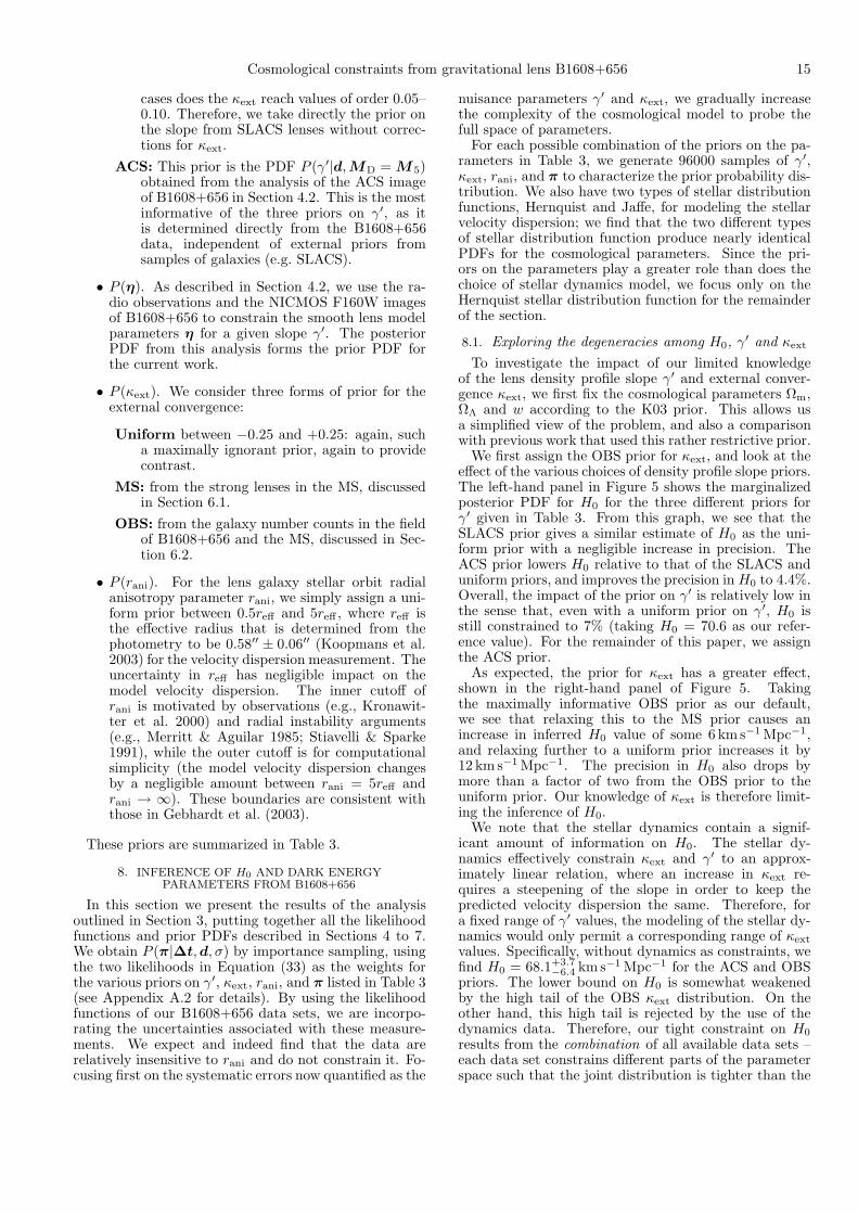
Cosmological constraints from gravitational lens B1608+656 15

cases does the κext reach values of order 0.05–0.10. Therefore, we take directly the prior onthe slope from SLACS lenses without correc-tions for κext.

ACS: This prior is the PDF P (γ′|d,MD = M 5)obtained from the analysis of the ACS imageof B1608+656 in Section 4.2. This is the mostinformative of the three priors on γ′, as itis determined directly from the B1608+656data, independent of external priors fromsamples of galaxies (e.g. SLACS).

• P (η). As described in Section 4.2, we use the ra-dio observations and the NICMOS F160W imagesof B1608+656 to constrain the smooth lens modelparameters η for a given slope γ′. The posteriorPDF from this analysis forms the prior PDF forthe current work.

• P (κext). We consider three forms of prior for theexternal convergence:

Uniform between −0.25 and +0.25: again, sucha maximally ignorant prior, again to providecontrast.

MS: from the strong lenses in the MS, discussedin Section 6.1.

OBS: from the galaxy number counts in the fieldof B1608+656 and the MS, discussed in Sec-tion 6.2.

• P (rani). For the lens galaxy stellar orbit radialanisotropy parameter rani, we simply assign a uni-form prior between 0.5reff and 5reff , where reff isthe effective radius that is determined from thephotometry to be 0.58′′ ± 0.06′′ (Koopmans et al.2003) for the velocity dispersion measurement. Theuncertainty in reff has negligible impact on themodel velocity dispersion. The inner cutoff ofrani is motivated by observations (e.g., Kronawit-ter et al. 2000) and radial instability arguments(e.g., Merritt & Aguilar 1985; Stiavelli & Sparke1991), while the outer cutoff is for computationalsimplicity (the model velocity dispersion changesby a negligible amount between rani = 5reff andrani → ∞). These boundaries are consistent withthose in Gebhardt et al. (2003).

These priors are summarized in Table 3.

8. INFERENCE OF H0 AND DARK ENERGYPARAMETERS FROM B1608+656

In this section we present the results of the analysisoutlined in Section 3, putting together all the likelihoodfunctions and prior PDFs described in Sections 4 to 7.We obtain P (π|∆t,d, σ) by importance sampling, usingthe two likelihoods in Equation (33) as the weights forthe various priors on γ′, κext, rani, and π listed in Table 3(see Appendix A.2 for details). By using the likelihoodfunctions of our B1608+656 data sets, we are incorpo-rating the uncertainties associated with these measure-ments. We expect and indeed find that the data arerelatively insensitive to rani and do not constrain it. Fo-cusing first on the systematic errors now quantified as the

nuisance parameters γ′ and κext, we gradually increasethe complexity of the cosmological model to probe thefull space of parameters.

For each possible combination of the priors on the pa-rameters in Table 3, we generate 96000 samples of γ′,κext, rani, and π to characterize the prior probability dis-tribution. We also have two types of stellar distributionfunctions, Hernquist and Jaffe, for modeling the stellarvelocity dispersion; we find that the two different typesof stellar distribution function produce nearly identicalPDFs for the cosmological parameters. Since the pri-ors on the parameters play a greater role than does thechoice of stellar dynamics model, we focus only on theHernquist stellar distribution function for the remainderof the section.

8.1. Exploring the degeneracies among H0, γ′ and κext

To investigate the impact of our limited knowledgeof the lens density profile slope γ′ and external conver-gence κext, we first fix the cosmological parameters Ωm,ΩΛ and w according to the K03 prior. This allows usa simplified view of the problem, and also a comparisonwith previous work that used this rather restrictive prior.

We first assign the OBS prior for κext, and look at theeffect of the various choices of density profile slope priors.The left-hand panel in Figure 5 shows the marginalizedposterior PDF for H0 for the three different priors forγ′ given in Table 3. From this graph, we see that theSLACS prior gives a similar estimate of H0 as the uni-form prior with a negligible increase in precision. TheACS prior lowers H0 relative to that of the SLACS anduniform priors, and improves the precision in H0 to 4.4%.Overall, the impact of the prior on γ′ is relatively low inthe sense that, even with a uniform prior on γ′, H0 isstill constrained to 7% (taking H0 = 70.6 as our refer-ence value). For the remainder of this paper, we assignthe ACS prior.

As expected, the prior for κext has a greater effect,shown in the right-hand panel of Figure 5. Takingthe maximally informative OBS prior as our default,we see that relaxing this to the MS prior causes anincrease in inferred H0 value of some 6 km s−1 Mpc−1,and relaxing further to a uniform prior increases it by12 km s−1 Mpc−1. The precision in H0 also drops bymore than a factor of two from the OBS prior to theuniform prior. Our knowledge of κext is therefore limit-ing the inference of H0.

We note that the stellar dynamics contain a signif-icant amount of information on H0. The stellar dy-namics effectively constrain κext and γ′ to an approx-imately linear relation, where an increase in κext re-quires a steepening of the slope in order to keep thepredicted velocity dispersion the same. Therefore, fora fixed range of γ′ values, the modeling of the stellar dy-namics would only permit a corresponding range of κext

values. Specifically, without dynamics as constraints, wefind H0 = 68.1+3.7

−6.4 km s−1 Mpc−1 for the ACS and OBSpriors. The lower bound on H0 is somewhat weakenedby the high tail of the OBS κext distribution. On theother hand, this high tail is rejected by the use of thedynamics data. Therefore, our tight constraint on H0

results from the combination of all available data sets –each data set constrains different parts of the parameterspace such that the joint distribution is tighter than the

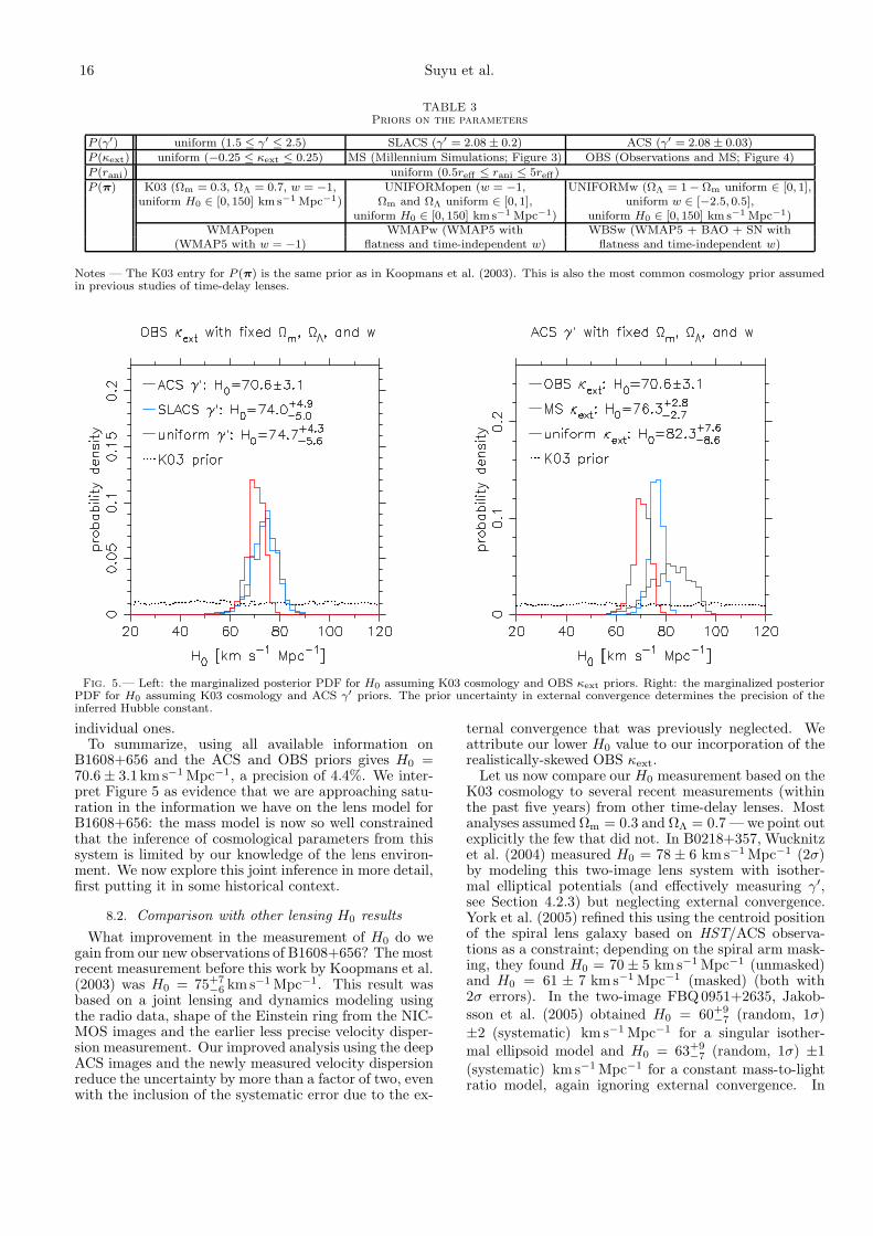
16 Suyu et al.

TABLE 3Priors on the parameters

P (γ′) uniform (1.5 ≤ γ′ ≤ 2.5) SLACS (γ′ = 2.08 ± 0.2) ACS (γ′ = 2.08 ± 0.03)

P (κext) uniform (−0.25 ≤ κext ≤ 0.25) MS (Millennium Simulations; Figure 3) OBS (Observations and MS; Figure 4)

P (rani) uniform (0.5reff ≤ rani ≤ 5reff )

P (π) K03 (Ωm = 0.3, ΩΛ = 0.7, w = −1, UNIFORMopen (w = −1, UNIFORMw (ΩΛ = 1 − Ωm uniform ∈ [0, 1],uniform H0 ∈ [0, 150] km s−1 Mpc−1) Ωm and ΩΛ uniform ∈ [0, 1], uniform w ∈ [−2.5, 0.5],

uniform H0 ∈ [0, 150] km s−1 Mpc−1) uniform H0 ∈ [0, 150] km s−1 Mpc−1)WMAPopen WMAPw (WMAP5 with WBSw (WMAP5 + BAO + SN with

(WMAP5 with w = −1) flatness and time-independent w) flatness and time-independent w)

Notes — The K03 entry for P (π) is the same prior as in Koopmans et al. (2003). This is also the most common cosmology prior assumedin previous studies of time-delay lenses.

Fig. 5.— Left: the marginalized posterior PDF for H0 assuming K03 cosmology and OBS κext priors. Right: the marginalized posteriorPDF for H0 assuming K03 cosmology and ACS γ′ priors. The prior uncertainty in external convergence determines the precision of theinferred Hubble constant.

individual ones.To summarize, using all available information on

B1608+656 and the ACS and OBS priors gives H0 =70.6 ± 3.1 km s−1 Mpc−1, a precision of 4.4%. We inter-pret Figure 5 as evidence that we are approaching satu-ration in the information we have on the lens model forB1608+656: the mass model is now so well constrainedthat the inference of cosmological parameters from thissystem is limited by our knowledge of the lens environ-ment. We now explore this joint inference in more detail,first putting it in some historical context.

8.2. Comparison with other lensing H0 results

What improvement in the measurement of H0 do wegain from our new observations of B1608+656? The mostrecent measurement before this work by Koopmans et al.(2003) was H0 = 75+7

−6 km s−1 Mpc−1. This result wasbased on a joint lensing and dynamics modeling usingthe radio data, shape of the Einstein ring from the NIC-MOS images and the earlier less precise velocity disper-sion measurement. Our improved analysis using the deepACS images and the newly measured velocity dispersionreduce the uncertainty by more than a factor of two, evenwith the inclusion of the systematic error due to the ex-

ternal convergence that was previously neglected. Weattribute our lower H0 value to our incorporation of therealistically-skewed OBS κext.

Let us now compare our H0 measurement based on theK03 cosmology to several recent measurements (withinthe past five years) from other time-delay lenses. Mostanalyses assumed Ωm = 0.3 and ΩΛ = 0.7 — we point outexplicitly the few that did not. In B0218+357, Wucknitzet al. (2004) measured H0 = 78 ± 6 km s−1 Mpc−1 (2σ)by modeling this two-image lens system with isother-mal elliptical potentials (and effectively measuring γ′,see Section 4.2.3) but neglecting external convergence.York et al. (2005) refined this using the centroid positionof the spiral lens galaxy based on HST/ACS observa-tions as a constraint; depending on the spiral arm mask-ing, they found H0 = 70 ± 5 km s−1 Mpc−1 (unmasked)and H0 = 61 ± 7 km s−1 Mpc−1 (masked) (both with2σ errors). In the two-image FBQ0951+2635, Jakob-sson et al. (2005) obtained H0 = 60+9

−7 (random, 1σ)

±2 (systematic) km s−1 Mpc−1 for a singular isother-mal ellipsoid model and H0 = 63+9

−7 (random, 1σ) ±1

(systematic) km s−1 Mpc−1 for a constant mass-to-lightratio model, again ignoring external convergence. In

Cosmological constraints from gravitational lens B1608+656 17

the two-image quasar system SDSS J1650+4251, Vuis-soz et al. (2007) found H0 = 51.7+4.0

−3.0 km s−1 Mpc−1 as-suming a singular isothermal sphere and constant exter-nal shear for the lens model. More general lens mod-els considered by these authors (e.g. including lens el-lipticity, or using a de Vaucouleurs density profile) werefound to be underconstrained. In the two-image quasarsystem SDSS J1206+4332, Paraficz et al. (2009) foundH0 = 73+3

−4 km s−1 Mpc−1 using singular isothermal el-lipsoids or spheres to describe the three lens galaxies,where photometry was used to place additional con-straints on the lens parameters. Recently, Fadely et al.(2009) modeled the gravitational lens Q0957+561 us-ing four different dark matter density profiles, each witha stellar component. The lens is embedded in a clus-ter, and the authors constrained the corresponding masssheet using the results of a weak lensing analysis byNakajima et al. (2009). Assuming a flat universe withΩm = 0.274 and cosmological constant ΩΛ = 0.726,they found H0 = 85+14

−13 km s−1 Mpc−1, where the prin-ciple uncertainties were due to the weakly constrainedstellar mass-to-light ratio (a manifestation of the radialprofile degeneracy in the lens model). Imposing con-straints from stellar population synthesis models led toH0 = 79.3+6.7

−8.5 km s−1 Mpc−1.17

In a nutshell, most of the recentH0 measurements fromindividual systems assumed isothermal profiles, and ne-glected the effects of both γ′ and κext: we interpret thesignificant variation between the H0 estimates in the re-cent literature as being due to these model limitations.In contrast, our B1608+656 analysis explicitly incorpo-rates the uncertainties due to our lack of knowledge ofboth γ′ and κext. In fact, a spread of ∼ 0.2 in γ′ around2.0 would give a spread of ∼ 40% in H0 for the caseswhere isothermal lenses are assumed (Wucknitz 2002).These in turn are set by a lack of information on the sys-tems, either because only two images are formed, or theextended source galaxy is not observed.

Other groups have looked to improve the constraintson H0 by combining several lenses together in a jointanalysis. Using a sample of 10 time-delay lenses, Sahaet al. (2006) measured H0 = 72+8

−11 km s−1 Mpc−1 bymodeling the lens’ convergence distributions on a gridand using the point image positions of the lenses as con-straints (the PixeLens method). Coles (2008) improvedon the method and obtained H0 = 71+6

−8 km s−1 Mpc−1

while addressing more clearly their prior assumptions.Oguri (2007) used a sample of 16 time-delay lenses toconstrain H0 = 68±6(stat.)±8(syst.) km s−1 Mpc−1 (forΩm = 0.24 and ΩΛ = 0.76; see footnote 17) by employinga statistical approach based on the image configurations.By simultaneously modeling SDSS J1206+4332 with fourother systems using PixeLens, Paraficz et al. (2009) de-rive H0 = 61.5+8

−4 km s−1 Mpc−1. The larger quoted errorbars on these ensemble estimates are perhaps a reflectionof the paucity of information available for each lens, asdiscussed above. All four analyses effectively assume thatthe ensemble external convergence distribution has zeromean, which may not be accurate: for example, Oguri(2007) constructed a sample for which external conver-gence could be neglected, and then incorporated this into

17 The corresponding H0 for the K03 cosmology is within ∼0.1% of the listed values.

the systematic error budget. Furthermore, Oguri (2007)imposed a Gaussian prior on the slope of γ′ = 2.00±0.15,and the PixeLens method’s priors on κ may well implic-itly impose constraints on γ that are similar to the priorin Oguri (2007); these priors on the slope may not beappropriate for individual systems in the ensembles.

In contrast, our measurement of γ′ from the ACS datameans that our results are independent of external pri-ors on γ′. In fact, our detailed study of the single well-observed lens B1608+656, even incorporating the effectsof κext, constrains H0 better than the studies using en-sembles of lenses. Our claim is that our analysis of thesystematic effects in B1608+656 — explicitly includingdensity profile slope and external convergence as nui-sance parameters — is one of the most extensive on asingle lens, and is rewarded with one of the most accu-rate measurements of H0 from time-delay lenses.

8.3. Relaxing the K03 prior

As we described in Section 2, strong lens time de-lays enable a measurement of a cosmological distance-like quantity, D∆t ≡ (1 + zd)DdDs/Dds. While there issome slight further dependence on cosmology in the stel-lar dynamics modeling, we expect this particular distancecombination to be well constrained by the system. To il-lustrate this, we plot in Figure 6 the PDF for D∆t withand without the constraints from B1608+656, for variouschoices of the cosmological parameter prior PDF. Specif-ically, we show the effect of relaxing the prior on Ωm,ΩΛ and w from the K03 delta function to the two typesof uniform distributions detailed in Table 3: “UNIFOR-Mopen” and “UNIFORMw”. We see that all of thesedistributions predict the same uninformative prior forD∆t, and that the B1608+656 posterior PDFs are cor-respondingly similar. With the OBS and ACS priors forκext and γ′, we estimate D∆t ' (5.16+0.29

−0.24) × 103 Mpc,a precision of ∼ 5%. The difference between the D∆t

estimates among the three priors shown is . 2%.Figure 6 suggests that a shifted log normal approxima-

tion (to take into account the skewness) for the productof the B1608+656 likelihood function, marginalized overthe OBS and ACS priors, is an appropriate compressionof our results. We find that

P (D∆t|H0,Ωm,ΩΛ, w) '1√

2π(x− λD)σD

exp

[

− (log(x− λD) − µD)2

2σ2D

]

, (35)

where x = D∆t/(1 Mpc), λD = 4000., µD = 7.053 andσD = 0.2282, accurately reproduces the cosmological pa-rameter inferences: for example, Hubble’s constant is re-covered to < 0.7% and its 16th and 84th percentiles (68%CL) are recovered to < 1.1% for the WMAP cosmologieswe considered.

8.4. Constraints on Ωm and ΩΛ

Based on the construction of D∆t, we expect stronglens time delays to be more sensitive to H0 than theother three cosmological parameters. This is shown inFigure 7, where we consider w = −1 uniform cosmolog-ical prior “UNIFORMopen” and plot the marginalizedB1608+656 posterior PDF to show the influence of thelensing data (blue lines). While there is a slight depen-dence on ΩΛ, we see that the B1608+656 data do indeed

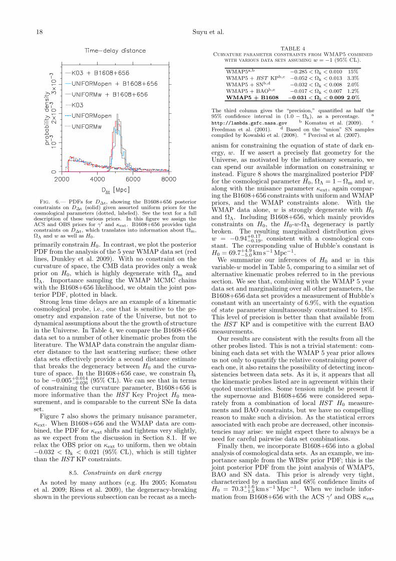
18 Suyu et al.

Fig. 6.— PDFs for D∆t, showing the B1608+656 posteriorconstraints on D∆t (solid) given assorted uniform priors for thecosmological parameters (dotted, labeled). See the text for a fulldescription of these various priors. In this figure we assign theACS and OBS priors for γ′ and κext. B1608+656 provides tightconstraints on D∆t, which translates into information about Ωm,ΩΛ and w as well as H0.

primarily constrainH0. In contrast, we plot the posteriorPDF from the analysis of the 5 year WMAP data set (redlines, Dunkley et al. 2009). With no constraint on thecurvature of space, the CMB data provides only a weakprior on H0, which is highly degenerate with Ωm andΩΛ. Importance sampling the WMAP MCMC chainswith the B1608+656 likelihood, we obtain the joint pos-terior PDF, plotted in black.

Strong lens time delays are an example of a kinematiccosmological probe, i.e., one that is sensitive to the ge-ometry and expansion rate of the Universe, but not todynamical assumptions about the the growth of structurein the Universe. In Table 4, we compare the B1608+656data set to a number of other kinematic probes from theliterature. The WMAP data constrain the angular diam-eter distance to the last scattering surface; these otherdata sets effectively provide a second distance estimatethat breaks the degeneracy between H0 and the curva-ture of space. In the B1608+656 case, we constrain Ωk

to be −0.005+0.014−0.026 (95% CL). We can see that in terms

of constraining the curvature parameter, B1608+656 ismore informative than the HST Key Project H0 mea-surement, and is comparable to the current SNe Ia dataset.

Figure 7 also shows the primary nuisance parameter,κext. When B1608+656 and the WMAP data are com-bined, the PDF for κext shifts and tightens very slightly,as we expect from the discussion in Section 8.1. If werelax the OBS prior on κext to uniform, then we obtain−0.032 < Ωk < 0.021 (95% CL), which is still tighterthan the HST KP constraints.

8.5. Constraints on dark energy

As noted by many authors (e.g. Hu 2005; Komatsuet al. 2009; Riess et al. 2009), the degeneracy-breakingshown in the previous subsection can be recast as a mech-

TABLE 4Curvature parameter constraints from WMAP5 combined

with various data sets assuming w = −1 (95% CL).

WMAP5a,b −0.285 < Ωk < 0.010 15%WMAP5 + HST KPb,c −0.052 < Ωk < 0.013 3.3%WMAP5 + SNb,d −0.032 < Ωk < 0.008 2.0%WMAP5 + BAOb,e −0.017 < Ωk < 0.007 1.2%WMAP5 + B1608 −0.031 < Ωk < 0.009 2.0%

The third column gives the “precision,” quantified as half the95% confidence interval in (1.0 − Ωk), as a percentage. a

http://lambda.gsfc.nasa.gov b Komatsu et al. (2009). c

Freedman et al. (2001). d Based on the “union” SN samplescompiled by Kowalski et al. (2008). e Percival et al. (2007).

anism for constraining the equation of state of dark en-ergy, w. If we assert a precisely flat geometry for theUniverse, as motivated by the inflationary scenario, wecan spend our available information on constraining winstead. Figure 8 shows the marginalized posterior PDFfor the cosmological parameter H0, ΩΛ = 1−Ωm and w,along with the nuisance parameter κext, again compar-ing the B1608+656 constraints with uniform and WMAPpriors, and the WMAP constraints alone. With theWMAP data alone, w is strongly degenerate with H0

and ΩΛ. Including B1608+656, which mainly providesconstraints on H0, the H0-w-ΩΛ degeneracy is partlybroken. The resulting marginalized distribution givesw = −0.94+0.17

−0.19, consistent with a cosmological con-stant. The corresponding value of Hubble’s constant isH0 = 69.7+4.9

−5.0 km s−1 Mpc−1.We summarize our inferences of H0 and w in this

variable-w model in Table 5, comparing to a similar set ofalternative kinematic probes referred to in the previoussection. We see that, combining with the WMAP 5 yeardata set and marginalizing over all other parameters, theB1608+656 data set provides a measurement of Hubble’sconstant with an uncertainty of 6.9%, with the equationof state parameter simultaneously constrained to 18%.This level of precision is better than that available fromthe HST KP and is competitive with the current BAOmeasurements.

Our results are consistent with the results from all theother probes listed. This is not a trivial statement: com-bining each data set with the WMAP 5 year prior allowsus not only to quantify the relative constraining power ofeach one, it also retains the possibility of detecting incon-sistencies between data sets. As it is, it appears that allthe kinematic probes listed are in agreement within theirquoted uncertainties. Some tension might be present ifthe supernovae and B1608+656 were considered sepa-rately from a combination of local HST H0 measure-ments and BAO constraints, but we have no compellingreason to make such a division. As the statistical errorsassociated with each probe are decreased, other inconsis-tencies may arise: we might expect there to always be aneed for careful pairwise data set combinations.

Finally then, we incorporate B1608+656 into a globalanalysis of cosmological data sets. As an example, we im-portance sample from the WBSw prior PDF; this is thejoint posterior PDF from the joint analysis of WMAP5,BAO and SN data. This prior is already very tight,characterized by a median and 68% confidence limits ofH0 = 70.3+1.6

−1.5 km s−1 Mpc−1. When we include infor-mation from B1608+656 with the ACS γ′ and OBS κext

Cosmological constraints from gravitational lens B1608+656 19

κ ext

0.0

0.12

0.24

H030 50 70 90 110

ΩΛ

0.0

0.4

0.8

Ωm

0.0

0.4

0.8

30 50 70 90 110

H0

Ωm0.2 0.6 1.0

flat

0.2 0.6 1.0

Ωm

ΩΛ0.2 0.6 1.0

0.2 0.6 1.0

ΩΛ

0.06 0.18 0.30

κext

0.06 0.18 0.30

κext

WMAPopen + B1608+656

WMAPopen

UNIFORMopen + B1608+656

Fig. 7.— The B1608+656 marginalized posterior PDF for H0, Ωm, ΩΛ and κext in a w = −1 cosmological model and assuming ACSγ′ and OBS κext priors; contours are 68% and 95% confidence levels. The three sets of colored contours correspond to three differentprior/data set combinations. Blue: B1608+656 constraints, given the UNIFORMopen prior; red: the prior provided by the WMAP 5 yeardata set alone; black: the joint constraints from combining WMAP and B1608+656. The blue contours in the Ωm and ΩΛ columns areomitted since they would show almost no constraints, as indicated by the diagonal panels.

priors, we obtain H0 = 70.4+1.5−1.4 km s−1 Mpc−1, a slight

shift in centroid and 6% reduction in the confidence in-terval. This is good as it shows global consistency in theWMAP5, BAO, SN and B1608+656 data sets.

8.6. Future prospects

In this paper, we have studied a single strong gravita-tional lens, B1608+656, investigating in depth the vari-ous model parameter degeneracies and systematic effects.At present, B1608+656 remains the only strong lens sys-tem with (i) time delay measurements with errors of onlya few percent, and (ii) extended source surface bright-ness distribution for accurate lens modeling; as we haveshown, these two properties together enable the carefulstudy and the resulting tight constraint on H0.

Table 5 shows that even this one system provides com-petitive accuracy on H0 and w for a single kinematicprobe, especially when we consider that all the other ex-periments involved averaging together many independentdistance measurements. What should we expect from ex-tending this study to many more lenses? As we showedin Section 8.1, if the data are good enough to constrainthe density profile slope to a few percent, the accuracyof the cosmological parameter inference is limited, as it

is in B1608+656, by our knowledge of the lens environ-ment, κext.

However, we also outlined in Section 6 how using infor-mation from numerical simulations and the photometryin the field can be used to constrain this nuisance param-eter and yield an unbiased estimate of H0. Furthermore,as discussed in Section 8.1, stellar dynamics provides sig-nificant amount of information on κext by limiting itspermissible range of values. While we, and also Treuet al. (2009) and Fassnacht et al. (2009), discuss how theline-of-sight contributions to κext should average to zeroover many lens systems, lens galaxies — like all mas-sive galaxies — tend to live in locally overdense environ-ments, such that the local contribution to κext would benon-zero. Careful studies of the lens environments (e.g.Momcheva et al. 2006; Fassnacht et al. 2006a; Blandfordet al. in preparation) and of N-body simulations with gasphysics to determine this local contribution to κext willbe crucial for obtaining H0 from a large sample of lenses.If we are able to average together N systems we should,in principle, be able to reduce our uncertainty by

√N .

In practice, the accuracy of the combination procedurewill sooner be limited by the systematic uncertainty inthe shape and centroid of the assumed κext distribution:

20 Suyu et al.

κ ext

0.0

0.12

0.24

H030 50 70 90 110

ΩΛ

0.0

0.4

0.8

w−

1.8

−1.

0

30 50 70 90 110

H0

w−1.8 −1.0 −0.2

−1.8 −1.0 −0.2

w

ΩΛ0.2 0.6 1.0

0.2 0.6 1.0

ΩΛ

0.06 0.18 0.30

κext

0.06 0.18 0.30

κext

WMAPw + B1608+656

WMAPw

UNIFORMw + B1608+656

Fig. 8.— The B1608+656 marginalized posterior PDF for H0, ΩΛ, w and κext in a flat cosmological model, again assuming ACS γ′ andOBS κext priors; contours are 68% and 95% confidence levels. The three sets of colored contours correspond to three different prior/dataset combinations. Blue: B1608+656 constraints, given the UNIFORMw prior; red: the prior provided by the WMAP 5 year data set alone;black: the joint constraints from combining WMAP and B1608+656. The blue contours in the Ωm and ΩΛ columns are omitted since theywould show almost no constraints, as indicated by the diagonal panels.

TABLE 5Dark energy constraints from WMAP5 combined with various data sets, assuming flat geometry.

H0/ km s−1 Mpc−1 w

WMAP5a,b 74+15−14 20% −1.06+0.41

−0.42 42%

WMAP5+HST KPa,b,c 72.1+7.4−7.6 10% −1.01+0.23

−0.22 23%

WMAP5+SNa,b,d 69.4+1.6−1.7 2.3% −0.977+0.065

−0.064 6.5%

WMAP5+BAOa,b,e 73.9+4.7−4.8 6.6% −1.15+0.21

−0.22 22%

WMAP5+Riessf 74.2 ± 3.6g 5.0% −1.12 ± 0.12 12%WMAP5+B1608 69.7+4.9

−5.0 6.9% −0.94+0.17

−0.1918%

The “precisions” in the third and fifth columns are defined as half the 68% confidence interval, as a percentage of either 72 for H0 or -1.0for w. a http://lambda.gsfc.nasa.gov b Komatsu et al. (2009). The H0 estimate was taken from the previously listed website. c

Freedman et al. (2001). d Based on the “union” SN samples compiled by Kowalski et al. (2008). e Percival et al. (2007). f Riess et al.(2009). g not marginalized over other cosmological parameters.

investigating the properties of this distribution is per-haps the most urgent topic for further work. Likewise, ifthe density profile slope cannot be constrained for eachtime-delay lens individually, the details of the prior PDFassigned for γ′ will become important as the ensemblegrows.

In the near future, cadenced surveys such as thoseplanned with the Large Synoptic Survey Telescope(LSST) and being undertaken by the Panoramic Survey

Telescope and Rapid Response System (Pan-STARRS)will discover large numbers of time-delay lenses, prompt-ing us to consider performing analyses such as the onedescribed here on hundreds of lens systems. In prac-tice, obtaining data of the quality we have presentedhere for hundreds of suitable lenses will pose a signifi-cant observational challenge. Nevertheless, Dobke et al.(2009), Coe & Moustakas (2009) and Oguri & Marshall(in preparation) investigate constraints on cosmological

Cosmological constraints from gravitational lens B1608+656 21

parameters based on large samples of time-delay lenses.In particular, Coe & Moustakas (2009) suggest that, interms of raw precision and in combination with a priorPDF from Planck, an LSST ensemble could reach sub-percent level precision in H0, and constrain w to 3% orbetter, provided that the systematic effects such as κext

are under control. Our work has already addressed someof these systematic effects, and will provide a basis forfuture analysis of large samples of time-delay lenses andlens environment studies.

9. CONCLUSIONS

We have studied the well-observed gravitational lensB1608+656 and used it to infer the values of cosmologi-cal parameters; we outlined and followed a Bayesian ap-proach for combining three data sets: HST/ACS imag-ing, stellar velocity dispersion measurement, and thetime delays between the multiple images. Diagnosingthe principal systematic effects, we included two nui-sance parameters (γ′ and κext) into the data model toaccount for them, assigning well-motivated prior PDFsand marginalizing over them. We draw the followingconclusions:

• We find that the HST/ACS images constrain thedensity profile slope parameter γ′ = 2.08 ± 0.03,which we propagate through the cosmological pa-rameter inference as a prior PDF. Relaxing thisprior to a uniform distribution degrades the preci-sion on H0 from 4.4% to 7.0%; the SLACS intrinsicprofile slope parameter distribution is not signifi-cantly more informative than the uniform prior.

• With the ACS prior for γ′, we find that the inferredcosmological parameters are dominated by the theexternal convergence κext. Ray-tracing through theMillennium Simulation gives a PDF for κext dueto line-of-sight contributions that has zero meanand width ∼ 0.04, while using the galaxy numbercounts in the B1608+656 field in conjunction withthe MS gives κext = 0.10+0.08

−0.05.

Using our most informative priors on the two nuisanceparameters, we arrive at the following cosmographic in-ferences:

• In the K03 cosmology (Ωm = 0.3, ΩΛ = 0.7,w = −1, and uniform H0), we obtain from theB1608+656 data set H0 = 70.6±3.1 km s−1 Mpc−1

(68% CL). The 4.4% error includes both statisti-cal and dominant systematic uncertainties, throughthe marginalization described above. This is a sig-nificant improvement to the earlier measurementof H0 = 75+7

−6 km s−1 Mpc−1 by Koopmans et al.(2003).

• Time-delay lenses are sensitive primarily to H0 butare weakly dependent on other cosmological pa-rameters; the lensing measurement of H0 is robustand useful for studying dark energy when combinedwith other cosmological probes. We find that forB1608+656 the cosmographic information can besummarized as a shifted log normal probability dis-tribution for the time-delay distance D∆t in unitsof Mpc, with the three parameters λD = 4000.,µD = 7.053 and σD = 0.2282.

• In a Λ-CDM cosmology (with w = −1), theB1608+656 data set breaks the degeneracy be-tween Ωm and ΩΛ in the WMAP 5 year data set,and constrains the curvature parameter to be zeroto 2.0% (95% CL), a level of precision similar tothose afforded by the current Type Ia SNe sample.

• B1608+656 in combination with the WMAP 5year data set, assuming flatness and allowing(a time-independent) w to vary, gives H0 =69.7+4.9

−5.0 km s−1 Mpc−1 and w = −0.94+0.17−0.19 (68%

CL).

These are significant improvements to the WMAP5only constraints of H0 = 74+15

−14 km s−1 Mpc−1 and

w = −1.06+0.41−0.42. B1608+656 is as competitive as

the current BAO data in determining w when com-bined with WMAP5.

Our detailed analysis of B1608+656 provides theframework for using large samples of time-delay lensesas cosmological probes in the near future. We anticipatethe local contribution to κext, which would not averageaway with a large sample of lenses, being the dominantresidual systematic error. Several lens environment stud-ies to circumvent this are underway; with the effects fromκext accurately modeled, future samples of time-delaygravitational lenses should be a competitive cosmologi-cal probe.

We thank M. Bradac, J. Hartlap, E. Komatsu,J. P. McKean and P. Schneider for useful discussions. Weare grateful to the anonymous referee whose suggestionsand comments helped clarify parts of the paper. S.H.S.is supported in part through the Deutsche Forschungsge-meinschaft under the project SCHN 342/7–1. C.D.F. ac-knowledge support under the HST program #GO-10158.Support for program #GO-10158 was provided by NASAthrough a grant from the Space Telescope Science In-stitute, which is operated by the Association of Uni-versities for Research in Astronomy, Inc., under NASAcontract NAS 5-26555. C.D.F. acknowledge the supportfrom the European Community’s Sixth Framework MarieCurie Research Training Network Programme, contractno. MRTN-CT-2004-505183 “ANGLES.” R.D.B. ac-knowledges support through NSF grant AST 05-07732.L.V.E.K. is supported in part through an NWO-VIDIcareer grant (project number 639.042.505). T.T. ac-knowledges support from the NSF through CAREERaward NSF-0642621, by the Sloan Foundation througha Sloan Research Fellowship, and by the Packard Foun-dation through a Packard Fellowship. This work was sup-ported in part by the NSF under award AST-0444059,the TABASGO foundation in the form of a research fel-lowship (P.J.M.), and by the US Department of Energyunder contract number DE-AC02-76SF00515. Based inpart on observations made with the NASA/ESA HubbleSpace Telescope, obtained at the Space Telescope ScienceInstitute, which is operated by the Association of Uni-versities for Research in Astronomy, Inc., under NASAcontract NAS 5-26555. These observations are associatedwith program #GO-10158.

22 Suyu et al.

REFERENCES

Auger, M. W., Fassnacht, C. D., Abrahamse, A. L., Lubin, L. M.,& Squires, G. K. 2007, AJ, 134, 668

Auger, M. W., Fassnacht, C. D., Wong, K. C., Thompson, D.,Matthews, K., & Soifer, B. T. 2008, ApJ, 673, 778

Barkana, R. 1998, ApJ, 502, 531Barnabe, M., Czoske, O., Koopmans, L. V. E., Treu, T., Bolton,

A. S., & Gavazzi, R. 2009, MNRAS, 399, 21Barnabe, M. & Koopmans, L. V. E. 2007, ApJ, 666, 726Binney, J. & Tremaine, S. 1987, Galactic dynamics (Princeton, NJ,

Princeton University Press, 1987, 747 p.)Bonamente, M., Joy, M. K., LaRoque, S. J., Carlstrom, J. E.,

Reese, E. D., & Dawson, K. S. 2006, ApJ, 647, 25Browne, I. W. A., Wilkinson, P. N., Jackson, N. J. F., Myers, S. T.,

Fassnacht, C. D., Koopmans, L. V. E., Marlow, D. R., Norbury,M., Rusin, D., Sykes, C. M., Biggs, A. D., Blandford, R. D., deBruyn, A. G., Chae, K.-H., Helbig, P., King, L. J., McKean,J. P., Pearson, T. J., Phillips, P. M., Readhead, A. C. S.,Xanthopoulos, E., & York, T. 2003, MNRAS, 341, 13

Coe, D. & Moustakas, L. A. 2009, ApJ, 706, 45Coles, J. 2008, ApJ, 679, 17Czoske, O., Barnabe, M., Koopmans, L. V. E., Treu, T., & Bolton,

A. S. 2008, MNRAS, 384, 987De Lucia, G. & Blaizot, J. 2007, MNRAS, 375, 2Dobke, B. M., King, L. J., Fassnacht, C. D., & Auger, M. W. 2009,

MNRAS, 397, 311Dunkley, J., Komatsu, E., Nolta, M. R., Spergel, D. N., Larson,

D., Hinshaw, G., Page, L., Bennett, C. L., Gold, B., Jarosik, N.,Weiland, J. L., Halpern, M., Hill, R. S., Kogut, A., Limon, M.,Meyer, S. S., Tucker, G. S., Wollack, E., & Wright, E. L. 2009,ApJS, 180, 306

Dye, S., Evans, N. W., Belokurov, V., Warren, S. J., & Hewett, P.2008, MNRAS, 388, 384

Dye, S. & Warren, S. J. 2005, ApJ, 623, 31Eisenstein, D. J., Zehavi, I., Hogg, D. W., Scoccimarro, R.,

Blanton, M. R., Nichol, R. C., Scranton, R., Seo, H.-J.,Tegmark, M., Zheng, Z., Anderson, S. F., Annis, J., Bahcall,N., Brinkmann, J., Burles, S., Castander, F. J., Connolly, A.,Csabai, I., Doi, M., Fukugita, M., Frieman, J. A., Glazebrook,K., Gunn, J. E., Hendry, J. S., Hennessy, G., Ivezic, Z., Kent, S.,Knapp, G. R., Lin, H., Loh, Y.-S., Lupton, R. H., Margon, B.,McKay, T. A., Meiksin, A., Munn, J. A., Pope, A., Richmond,M. W., Schlegel, D., Schneider, D. P., Shimasaku, K., Stoughton,C., Strauss, M. A., SubbaRao, M., Szalay, A. S., Szapudi, I.,Tucker, D. L., Yanny, B., & York, D. G. 2005, ApJ, 633, 560

Fadely, R., Keeton, C. R., Nakajima, R., & Bernstein, G. M. 2009,ArXiv e-prints (0909.1807)

Falco, E. E., Gorenstein, M. V., & Shapiro, I. I. 1985, ApJ, 289,L1

Fassnacht, C. D., Gal, R. R., Lubin, L. M., McKean, J. P., Squires,G. K., & Readhead, A. C. S. 2006a, ApJ, 642, 30

Fassnacht, C. D., Koopmans, L. V. E., & Wong, K. C. 2009, ArXive-prints (0909.4301)

Fassnacht, C. D., McKean, J. P., Koopmans, L. V. E., Treu, T.,Blandford, R. D., Auger, M. W., Jeltema, T. E., Lubin, L. M.,Margoniner, V. E., & Wittman, D. 2006b, ApJ, 651, 667

Fassnacht, C. D., Pearson, T. J., Readhead, A. C. S., Browne,I. W. A., Koopmans, L. V. E., Myers, S. T., & Wilkinson, P. N.1999, ApJ, 527, 498

Fassnacht, C. D., Womble, D. S., Neugebauer, G., Browne, I. W. A.,Readhead, A. C. S., Matthews, K., & Pearson, T. J. 1996, ApJ,460, L103

Fassnacht, C. D., Xanthopoulos, E., Koopmans, L. V. E., & Rusin,D. 2002, ApJ, 581, 823

Freedman, W. L., Madore, B. F., Gibson, B. K., Ferrarese, L.,Kelson, D. D., Sakai, S., Mould, J. R., Kennicutt, Jr., R. C.,Ford, H. C., Graham, J. A., Huchra, J. P., Hughes, S. M. G.,Illingworth, G. D., Macri, L. M., & Stetson, P. B. 2001, ApJ,553, 47

Gavazzi, R., Treu, T., Koopmans, L. V. E., Bolton, A. S.,Moustakas, L. A., Burles, S., & Marshall, P. J. 2008, ApJ, 677,1046

Gavazzi, R., Treu, T., Rhodes, J. D., Koopmans, L. V. E., Bolton,A. S., Burles, S., Massey, R. J., & Moustakas, L. A. 2007, ApJ,667, 176

Gebhardt, K., Richstone, D., Tremaine, S., Lauer, T. R., Bender,R., Bower, G., Dressler, A., Faber, S. M., Filippenko, A. V.,Green, R., Grillmair, C., Ho, L. C., Kormendy, J., Magorrian,J., & Pinkney, J. 2003, ApJ, 583, 92

Grogin, N. A. & Narayan, R. 1996a, ApJ, 464, 92—. 1996b, ApJ, 473, 570Hernquist, L. 1990, ApJ, 356, 359Herrnstein, J. R., Moran, J. M., Greenhill, L. J., Diamond, P. J.,

Inoue, M., Nakai, N., Miyoshi, M., Henkel, C., & Riess, A. 1999,Nature, 400, 539

Hicken, M., Wood-Vasey, W. M., Blondin, S., Challis, P., Jha, S.,Kelly, P. L., Rest, A., & Kirshner, R. P. 2009, ApJ, 700, 1097

Hilbert, S., Hartlap, J., White, S. D. M., & Schneider, P. 2009,A&A, 499, 31

Hilbert, S., White, S. D. M., Hartlap, J., & Schneider, P. 2007,MNRAS, 382, 121

—. 2008, MNRAS, 386, 1845Hu, W. 2005, 339, 215Humphrey, P. J. & Buote, D. A. 2009, ArXiv e-prints (0911.0678)Jaffe, W. 1983, MNRAS, 202, 995Jakobsson, P., Hjorth, J., Burud, I., Letawe, G., Lidman, C., &

Courbin, F. 2005, A&A, 431, 103Keeton, C. R. & Zabludoff, A. I. 2004, ApJ, 612, 660Kirshner, R. P. & Kwan, J. 1974, ApJ, 193, 27Kochanek, C. S. 2002, ApJ, 578, 25Komatsu, E., Dunkley, J., Nolta, M. R., Bennett, C. L., Gold,

B., Hinshaw, G., Jarosik, N., Larson, D., Limon, M., Page, L.,Spergel, D. N., Halpern, M., Hill, R. S., Kogut, A., Meyer, S. S.,Tucker, G. S., Weiland, J. L., Wollack, E., & Wright, E. L. 2009,ApJS, 180, 330

Koopmans, L. V. E., Bolton, A., Treu, T., Czoske, O., Auger,M. W., Barnabe, M., Vegetti, S., Gavazzi, R., Moustakas, L. A.,& Burles, S. 2009, ApJ, 703, L51

Koopmans, L. V. E. & Treu, T. 2002, ApJ, 568, L5Koopmans, L. V. E., Treu, T., Bolton, A. S., Burles, S., &

Moustakas, L. A. 2006, ApJ, 649, 599Koopmans, L. V. E., Treu, T., Fassnacht, C. D., Blandford, R. D.,

& Surpi, G. 2003, ApJ, 599, 70Kowalski, M., Rubin, D., Aldering, G., Agostinho, R. J., Amadon,

A., Amanullah, R., Balland, C., Barbary, K., Blanc, G., Challis,P. J., Conley, A., Connolly, N. V., Covarrubias, R., Dawson,K. S., Deustua, S. E., Ellis, R., Fabbro, S., Fadeyev, V., Fan,X., Farris, B., Folatelli, G., Frye, B. L., Garavini, G., Gates,E. L., Germany, L., Goldhaber, G., Goldman, B., Goobar, A.,Groom, D. E., Haissinski, J., Hardin, D., Hook, I., Kent, S.,Kim, A. G., Knop, R. A., Lidman, C., Linder, E. V., Mendez, J.,Meyers, J., Miller, G. J., Moniez, M., Mourao, A. M., Newberg,H., Nobili, S., Nugent, P. E., Pain, R., Perdereau, O., Perlmutter,S., Phillips, M. M., Prasad, V., Quimby, R., Regnault, N.,Rich, J., Rubenstein, E. P., Ruiz-Lapuente, P., Santos, F. D.,Schaefer, B. E., Schommer, R. A., Smith, R. C., Soderberg,A. M., Spadafora, A. L., Strolger, L.-G., Strovink, M., Suntzeff,N. B., Suzuki, N., Thomas, R. C., Walton, N. A., Wang, L.,Wood-Vasey, W. M., & Yun, J. L. 2008, ApJ, 686, 749

Kronawitter, A., Saglia, R. P., Gerhard, O., & Bender, R. 2000,A&AS, 144, 53

Lewis, A. & Bridle, S. 2002, Phys. Rev. D, 66, 103511MacKay, D. 2003, Information Theory, Inference and Learning

Algorithms (Cambridge: CUP)Macri, L. M., Stanek, K. Z., Bersier, D., Greenhill, L. J., & Reid,

M. J. 2006, ApJ, 652, 1133McKean, J. P., Auger, M. W., Koopmans, L. V. E., Vegetti, S.,

Czoske, O., Fassnacht, C. D., Treu, T., More, A., & Kocevski,D. D. 2009, ArXiv e-prints (0910.1133)

Merritt, D. 1985, AJ, 90, 1027Merritt, D. & Aguilar, L. A. 1985, MNRAS, 217, 787Momcheva, I., Williams, K., Keeton, C., & Zabludoff, A. 2006,

ApJ, 641, 169Myers, S. T., Fassnacht, C. D., Djorgovski, S. G., Blandford,

R. D., Matthews, K., Neugebauer, G., Pearson, T. J., Readhead,A. C. S., Smith, J. D., Thompson, D. J., Womble, D. S., Browne,I. W. A., Wilkinson, P. N., Nair, S., Jackson, N., Snellen, I. A. G.,Miley, G. K., de Bruyn, A. G., & Schilizzi, R. T. 1995, ApJ, 447,L5

Cosmological constraints from gravitational lens B1608+656 23

Myers, S. T., Jackson, N. J., Browne, I. W. A., de Bruyn, A. G.,Pearson, T. J., Readhead, A. C. S., Wilkinson, P. N., Biggs,A. D., Blandford, R. D., Fassnacht, C. D., Koopmans, L. V. E.,Marlow, D. R., McKean, J. P., Norbury, M. A., Phillips, P. M.,Rusin, D., Shepherd, M. C., & Sykes, C. M. 2003, MNRAS, 341,1

Nakajima, R., Bernstein, G. M., Fadely, R., Keeton, C. R., &Schrabback, T. 2009, ApJ, 697, 1793

Oguri, M. 2007, ApJ, 660, 1Oke, J. B., Cohen, J. G., Carr, M., Cromer, J., Dingizian, A.,

Harris, F. H., Labrecque, S., Lucinio, R., Schaal, W., Epps, H.,& Miller, J. 1995, PASP, 107, 375

Osipkov, L. P. 1979, Pis ma Astronomicheskii Zhurnal, 5, 77

Paraficz, D., Hjorth, J., & Elıasdottir, A. 2009, A&A, 499, 395Percival, W. J., Cole, S., Eisenstein, D. J., Nichol, R. C., Peacock,

J. A., Pope, A. C., & Szalay, A. S. 2007, MNRAS, 381, 1053Perlmutter, S., Aldering, G., Goldhaber, G., Knop, R. A., Nugent,

P., Castro, P. G., Deustua, S., Fabbro, S., Goobar, A., Groom,D. E., Hook, I. M., Kim, A. G., Kim, M. Y., Lee, J. C., Nunes,N. J., Pain, R., Pennypacker, C. R., Quimby, R., Lidman,C., Ellis, R. S., Irwin, M., McMahon, R. G., Ruiz-Lapuente,P., Walton, N., Schaefer, B., Boyle, B. J., Filippenko, A. V.,Matheson, T., Fruchter, A. S., Panagia, N., Newberg, H. J. M.,Couch, W. J., & The Supernova Cosmology Project. 1999, ApJ,517, 565

Refsdal, S. 1964, MNRAS, 128, 307Riess, A. G., Filippenko, A. V., Challis, P., Clocchiatti, A., Diercks,

A., Garnavich, P. M., Gilliland, R. L., Hogan, C. J., Jha, S.,Kirshner, R. P., Leibundgut, B., Phillips, M. M., Reiss, D.,Schmidt, B. P., Schommer, R. A., Smith, R. C., Spyromilio, J.,Stubbs, C., Suntzeff, N. B., & Tonry, J. 1998, AJ, 116, 1009

Riess, A. G., Macri, L., Casertano, S., Sosey, M., Lampeitl, H.,Ferguson, H. C., Filippenko, A. V., Jha, S. W., Li, W., Chornock,R., & Sarkar, D. 2009, ApJ, 699, 539

Saha, P., Coles, J., Maccio, A. V., & Williams, L. L. R. 2006, ApJ,650, L17

Schmidt, B. P., Kirshner, R. P., Eastman, R. G., Phillips, M. M.,Suntzeff, N. B., Hamuy, M., Maza, J., & Aviles, R. 1994, ApJ,432, 42

Schneider, P., Kochanek, C. S., & Wambsganss, J. 2006,Gravitational Lensing: Strong, Weak and Micro (Springer)

Sivia, D. S. 1996, Data Analysis: A Bayesian Tutorial (Oxford:OUP)

Spergel, D. N., Bean, R., Dore, O., Nolta, M. R., Bennett, C. L.,Dunkley, J., Hinshaw, G., Jarosik, N., Komatsu, E., Page, L.,Peiris, H. V., Verde, L., Halpern, M., Hill, R. S., Kogut, A.,Limon, M., Meyer, S. S., Odegard, N., Tucker, G. S., Weiland,J. L., Wollack, E., & Wright, E. L. 2007, ApJS, 170, 377

Springel, V., White, S. D. M., Jenkins, A., Frenk, C. S., Yoshida,N., Gao, L., Navarro, J., Thacker, R., Croton, D., Helly, J.,Peacock, J. A., Cole, S., Thomas, P., Couchman, H., Evrard,A., Colberg, J., & Pearce, F. 2005, Nature, 435, 629

Stiavelli, M. & Sparke, L. S. 1991, ApJ, 382, 466Sunyaev, R. A. & Zel’dovich, I. B. 1980, ARA&A, 18, 537Suyu, S. H., Marshall, P. J., Blandford, R. D., Fassnacht, C. D.,

Koopmans, L. V. E., McKean, J. P., & Treu, T. 2009, ApJ, 691,277

Suyu, S. H., Marshall, P. J., Hobson, M. P., & Blandford, R. D.2006, MNRAS, 371, 983

Tammann, G. A. 1979, in NASA Conference Publication, Vol. 2111,NASA Conference Publication, 263–293

Tonry, J. L. & Franx, M. 1999, ApJ, 515, 512Treu, T., Gavazzi, R., Gorecki, A., Marshall, P. J., Koopmans,

L. V. E., Bolton, A. S., Moustakas, L. A., & Burles, S. 2009,ApJ, 690, 670

Treu, T., Koopmans, L. V., Bolton, A. S., Burles, S., & Moustakas,L. A. 2006, ApJ, 640, 662

Treu, T. & Koopmans, L. V. E. 2002, MNRAS, 337, L6van der Marel, R. P. 1994, MNRAS, 270, 271Vuissoz, C., Courbin, F., Sluse, D., Meylan, G., Chantry, V.,

Eulaers, E., Morgan, C., Eyler, M. E., Kochanek, C. S., Coles,J., Saha, P., Magain, P., & Falco, E. E. 2008, A&A, 488, 481

Vuissoz, C., Courbin, F., Sluse, D., Meylan, G., Ibrahimov, M.,Asfandiyarov, I., Stoops, E., Eigenbrod, A., Le Guillou, L., vanWinckel, H., & Magain, P. 2007, A&A, 464, 845

Wucknitz, O. 2002, MNRAS, 332, 951Wucknitz, O., Biggs, A. D., & Browne, I. W. A. 2004, MNRAS,

349, 14

York, T., Jackson, N., Browne, I. W. A., Wucknitz, O., & Skelton,J. E. 2005, MNRAS, 357, 124

APPENDIX

A. PROBABILITY THEORY FOR MEASURING COSMOLOGICAL PARAMETERS

In this appendix, we describe how we derive the expressions for the likelihoods of the time delay and the ACSdata sets stated in Section 3.3. We also provide the details on the sampling techniques for calculating the posteriorprobability density of cosmological parameters.

A.1. Simplification of the likelihoods

For B1608+656, we can simplify the marginalization of the likelihoods P (∆t|ξ) and P (d|ξ) in Equation (24) basedon the following facts, which are either from Paper I or shown in Section 4:

• from Paper I, the top MD models led to equal evidence values P (d|γ′,η, δψMP,MD) (within the uncertainties).

• in Section 4, the likelihood function P (∆t|ξ) is approximately constant for these top MD models for a givencosmology.

• in Section 4, for good data modelsMD of B1608+656, the potential corrections δψ do not change significantly thepredicted values of the Fermat potential, i.e., the simply-parametrized SPLE initial model provides an unbiasedestimator for the Fermat potential.

• the likelihood P (σ|ξ) is also constant for the various MD because the dynamics modeling is independent of thelensed image processing models MD.

• simulations suggest that the potential corrections δψ are sharply peaked about the most probable values δψMP.

With the above results, the Fermat potential can be more easily computed from the SPLE model: there is a strongcorrelation between the ∆φ and γ′, and we obtain the relation between ∆φ and γ′ by evaluating them at severaldiscrete γ′ values and interpolating between them. For notational simplicity, we consequently drop the nearly-trueindependences of ∆φ on η and δψ. In computing the predicted ∆φ, the average source position of the four mapped(via the lens equation) image positions on the source plane is used. Denoting the dependence of ∆φ on γ′ for κext = 0

24 Suyu et al.

and a given MD as q(γ′,MD) and using the mass-sheet degeneracy relation for the dependence of ∆φ on κext, weobtain Equations (25) through (27) for the likelihood of the time delay data.18

For the likelihood of the ACS data, we work with the SPLE potential model on the basis that the Fermat potentialis insensitive to the potential corrections and the potential corrections only slightly alter the ranking of MD models.We can choose the MD to be one of the top models, say M5 (since the normalization in P (π|∆t,d, σ) is irrelevant),and drop the dependence on δψ in the likelihood of the ACS data to simplify part of the integrand in Equation (24):

∫

dδψ ds dMD P (d|γ′,η, δψ, s,MD) ·

P (s|λ, g)P (MD)P (δψ)

∝∼∫

ds P (d|γ′,η, s,MD = M5)P (s|λ, g)

=P (d|γ′,η,MD =M 5), (A1)

which is also Equation (29). In deriving the above equation, we assume that the representative set of models MD

obtained in Suyu et al. (2009) are equally probable a priori (i.e., the prior P (MD) is constant). For the priorsP (s|λ, g) and P (δψ), we use quadratic forms of the regularizing function. Specifically, we try zeroth-order, gradientand curvature forms for P (s|λ, g), and the curvature form for P (δψ), as described in Suyu et al. (2006) and Suyuet al. (2009). As a reminder, the quantity P (d|γ′,η,MD = M5) is the Bayesian evidence from source reconstructiongiven the lens model parameters γ′, η and the data model M5; this evidence value is calculable based on Suyu et al.(2009).

A.2. Importance sampling

In practice, we can incorporate the various likelihoods in Equation (33) by importance sampling the prior distribution(see e.g. Lewis & Bridle 2002, for an introduction). This is a method for calculating integrals over a PDF P2 whenall we have is samples drawn from some other PDF P1. Consider the expectation value of a parameter x:

〈x〉2 =

∫

x · P2(x) dx, (A2)

=

∫

xP2(x)

P1(x)· P1(x) dx. (A3)

The process of weighting the samples from P1 by the ratio P2(x)/P1(x) is called importance sampling. It works mostefficiently when P1 and P2 are quite similar, and fails if P1 is zero-valued over some of the range of P2, or if thesampling of P1 is too sparse.

In our case, we would like to calculate integrals over, for example, P2 = P (π, γ′, κext, rani|∆t,d, σ), while the prioris written simply P1 = P (π, γ′, κext, rani|d) (recall that d is used to provide a prior on γ′). Using Bayes’ theorem, wecan write

P (π, γ′, κext, rani|∆t,d, σ) ∝P (∆t, σ|π, γ′, κext, rani)P (π, γ′, κext, rani|d),

i.e. P2 ∝ P (∆t, σ|π, γ′, κext, rani)P1. (A4)

From this we can see that the weight we must attach to each sample from the prior is just the value of the likelihoodP (∆t, σ|π, γ′, κext, rani). Note that these weights can be rescaled by an arbitrary factor, which can be important inretaining numerical stability.

We apply this technique to perform the marginalization in Equation (33). Specifically, we have samples of P (π),P (γ′|d,MD = M5), P (κext) and P (rani), and employ importance sampling to obtain P (π|∆t,d, σ).

18 The Fermat potential is independent of cosmological parameters because we work in terms of the scaled lens potential in angular(arcsecond) units. Cosmological parameters and redshifts are only needed for deriving physical quantities of the lens system, such asthe one-dimensional velocity dispersion (calculable from the Einstein radius) of the lens, mass of the lens, and the physical extent of thelens/source.