AJ, in pressPreprint typeset using LATEX style emulateapj v. 12/16/11

THE DATA REDUCTION PIPELINE FOR THE SDSS-IV MANGA IFU GALAXY SURVEY

David R. Law1, Brian Cherinka2, Renbin Yan3, Brett H. Andrews4, Matthew A. Bershady5, Dmitry Bizyaev6,Guillermo A. Blanc7,8,9, Michael R. Blanton10, Adam S. Bolton11, Joel R. Brownstein11, Kevin Bundy12,

Yanmei Chen13,14, Niv Drory15, Richard D’Souza16, Hai Fu17, Amy Jones16, Guinevere Kauffmann16, NicholasMacDonald18, Karen L. Masters19, Jeffrey A. Newman4, John K. Parejko18, Jose R. Sanchez-Gallego3,

Sebastian F. Sanchez20, David J. Schlegel21, Daniel Thomas19, David A. Wake5,22, Anne-Marie Weijmans23, KyleB. Westfall19, Kai Zhang3

AJ, in press

ABSTRACT

Mapping Nearby Galaxies at Apache Point Observatory (MaNGA) is an optical fiber-bundle integral-field unit (IFU) spectroscopic survey that is one of three core programs in the fourth-generationSloan Digital Sky Survey (SDSS-IV). With a spectral coverage of 3622 – 10,354 A and an averagefootprint of ∼ 500 arcsec2 per IFU the scientific data products derived from MaNGA will permitexploration of the internal structure of a statistically large sample of 10,000 low redshift galaxies inunprecedented detail. Comprising 174 individually pluggable science and calibration IFUs with anear-constant data stream, MaNGA is expected to obtain ∼ 100 million raw-frame spectra and ∼ 10million reduced galaxy spectra over the six-year lifetime of the survey. In this contribution, we describethe MaNGA Data Reduction Pipeline (DRP) algorithms and centralized metadata framework thatproduces sky-subtracted, spectrophotometrically calibrated spectra and rectified 3-D data cubes thatcombine individual dithered observations. For the 1390 galaxy data cubes released in Summer 2016 aspart of SDSS-IV Data Release 13 (DR13), we demonstrate that the MaNGA data have nearly Poisson-limited sky subtraction shortward of ∼ 8500 A and reach a typical 10σ limiting continuum surfacebrightness µ = 23.5 AB arcsec−2 in a five arcsec diameter aperture in the g band. The wavelengthcalibration of the MaNGA data is accurate to 5 km s−1 rms, with a median spatial resolution of 2.54arcsec FWHM (1.8 kpc at the median redshift of 0.037) and a median spectral resolution of σ = 72km s−1.Keywords: methods: data analysis — surveys — techniques: imaging spectroscopy

1 Space Telescope Science Institute, 3700 San Martin Drive,Baltimore, MD 21218, USA (dlaw@stsci.edu)

2 Center for Astrophysical Sciences, Department of Physicsand Astronomy, Johns Hopkins University, Baltimore, MD21218, USA

3 Department of Physics and Astronomy, University of Ken-tucky, 505 Rose Street, Lexington, KY 40506-0055, USA

4 Department of Physics and Astronomy and PITT PACC,University of Pittsburgh, 3941 O’Hara St., Pittsburgh, PA15260, USA

5 Department of Astronomy, University of Wisconsin-Madison, 475 N. Charter Street, Madison, WI, 53706, USA

6 Apache Point Observatory, P.O. Box 59, Sunspot, NM 88349,USA

7 Departamento de Astronomıa, Universidad de Chile, Caminodel Observatorio 1515, Las Condes, Santiago, Chile

8 Centro de Astrofısica y Tecnologıas Afines (CATA), Caminodel Observatorio 1515, Las Condes, Santiago, Chile

9 Visiting Astronomer, Observatories of the Carnegie Institu-tion for Science, 813 Santa Barbara St, Pasadena, CA, 91101,USA

10 Center for Cosmology and Particle Physics, Department ofPhysics, New York University, 4 Washington Place, New York,NY 10003

11 Department of Physics and Astronomy, University of Utah,115 S 1400 E, Salt Lake City, UT 84112, USA

12 Kavli Institute for the Physics and Mathematics of the Uni-verse, Todai Institutes for Advanced Study, the University ofTokyo, Kashiwa, Japan 277-8583 (Kavli IPMU, WPI)

13 School of Astronomy and Space Science, Nanjing Univer-sity, Nanjing 210093, China

14 Key Laboratory of Modern Astronomy and Astrophysics(Nanjing University), Ministry of Education, Nanjing 210093,China

15 McDonald Observatory, Department of Astronomy, Univer-sity of Texas at Austin, 1 University Station, Austin, TX 78712-

0259, USA16 Max Planck Institute for Astrophysics, Karl-Schwarzschild-

Str. 1, D-85748 Garching, Germany17 Department of Physics & Astronomy, University of Iowa,

Iowa City, IA 52242, USA18 Department of Astronomy, Box 351580, University of Wash-

ington, Seattle, WA 98195, USA19 Institute of Cosmology and Gravitation, University of

Portsmouth, Portsmouth, UK20 Instituto de Astronomia, Universidad Nacional Autonoma

de Mexico, A.P. 70-264, 04510 Mexico D.F., Mexico21 Physics Division, Lawrence Berkeley National Laboratory,

Berkeley, CA 94720-816022 Department of Physical Sciences, The Open University, Mil-

ton Keynes, UK23 School of Physics and Astronomy, University of St Andrews,

North Haugh, St Andrews KY16 9SS, UK

2 Law et al.

1. INTRODUCTION

Over the last twenty years, multiplexed spectroscopicsurveys have been valuable tools for bringing the powerof statistics to bear on the study of galaxy formation.Using large samples of tens to hundreds of thousands ofgalaxies with optical spectroscopy from the Sloan Digi-tal Sky Survey (York et al. 2000; Abazajian et al. 2003)for instance, studies have outlined fundamental relationsbetween stellar mass, metallicity, element abundance ra-tios, and star formation history (e.g., Kauffmann et al.2003; Tremonti et al. 2004; Thomas et al. 2010). How-ever, this statistical power has historically come at thecost of treating galaxies as point sources, with only asmall and biased region subtended by a given optical fibercontributing to the recorded spectrum.

As technology has advanced, techniques have been de-veloped for imaging spectroscopy that allow simultane-ous spatial and spectral coverage, with correspondinglygreater information density for each individual galaxy.Building on early work by (e.g.) Colina et al. (1999) andde Zeeuw et al. (2002), such integral-field spectroscopyhas provided a wealth of information. In the nearby uni-verse for instance, observations from the DiskMass sur-vey (Bershady et al. 2010) have indicated that late-typegalaxies tend to have sub-maximal disks (Bershady etal. 2011), while Atlas-3D observations (Cappellari et al.2011a) showed that early-type galaxies frequently haverapidly-rotating components (especially in low densityenvironments; Cappellari et al. 2011b). In the moredistant universe, integral-field spectroscopic observationshave been crucial in establishing the prevalence of highgas-phase velocity dispersions (e.g., Forster Schreiber etal. 2009; Law et al. 2009, 2012; Wisnioski et al. 2015), gi-ant kiloparsec-sized clumps of young stars (e.g., ForsterSchreiber et al. 2011), and powerful nuclear outflows(Forster Schreiber et al. 2014) that may indicate fun-damental differences in gas accretion mechanisms in theyoung universe (e.g., Dekel et al. 2009).

More recently, surveys such as CALIFA (Calar AltoLegacy Integral Field Area Survey, Sanchez et al. 2012;Garcıa-Benito et al. 2015), SAMI (Sydney-AAO Multi-object IFS, Croom et al. 2012; Allen et al. 2015), andMaNGA (Mapping Nearby Galaxies at APO, Bundy etal. 2015) have begun to combine the information densityof integral field spectroscopy with the statistical powerof large multiplexed samples. As a part of the 4th gen-eration of the Sloan Digital Sky Survey (SDSS-IV), theMaNGA project bundles single fibers from the BaryonOscillation Spectroscopic Survey (BOSS) spectrograph(Smee et al. 2013) into integral-field units (IFUs); overthe six-year lifetime of the survey (2014-2020) MaNGAwill obtain spatially resolved optical+NIR spectroscopyof 10,000 galaxies at redshifts z ∼ 0.02−0.1. In additionto providing insight into the resolved structure of stellarpopulations, galactic winds, and dynamical evolution inthe local universe (e.g., Belfiore et al. 2015; Li et al. 2015;Wilkinson et al. 2015), the MaNGA data set will be aninvaluable legacy product with which to help understandgalaxies in the distant universe. As next-generation fa-cilities come online in the final years of the MaNGA sur-vey, IFU spectrographs such as TMT/IRIS (Moore et al.2014; Wright et al. 2014), JWST/NIRSPEC (Closs etal. 2008; Birkmann et al. 2014), and JWST/MIRI-MRS

(Wells et al. 2015) will trace the crucial rest-optical band-pass in galaxies out to redshift z ∼ 10 and beyond.

Imaging spectroscopic surveys such as MaNGA facesubstantial calibration challenges in order to meetthe science requirements of the survey (Yan et al.2016b). In addition to requiring accurate absolutespectrophotometry from each fiber, MaNGA must cor-rect for gravitationally-induced flexure variability in theCassegrain-mounted BOSS spectrographs, determine ac-curate micron-precision astrometry for each IFU bundle,and combine spectra from the individual fibers with ac-curate astrometric information in order to construct 3-Ddata cubes that rectify the wavelength-dependent differ-ential atmospheric refraction and (despite large intersti-tial gaps in the fiber bundles) consistently deliver high-quality imaging products. These combined requirementshave driven a substantial software pipeline developmenteffort throughout the early years of SDSS-IV.

Historically, IFU data have been processed with a mix-ture of software tools ranging from custom built pipelines(e.g., Zanichelli et al. 2005) to general purpose tools ca-pable of performing all or part of the basic data reductiontasks for multiple IFUs. For fiber-fed IFUs (with or with-out coupled lenslet arrays) that deliver a pseudo-slit ofdiscrete apertures the raw data is similar in format totraditional multiobject spectroscopy and has hence beenable to build upon an existing code base. In contrast,slicer-based IFUs produce data in a format more akin tolong-slit spectroscopy, while pure-lenslet IFUs are differ-ent altogether with individual spectra staggered acrossthe detector.

Following Sandin et al. (2010), we provide here a briefoverview of some of the common tools for the reductionof data from optical and near-IR IFUs (see also Bershady2009), including both fiber-fed IFUs with data formatssimilar to MaNGA and lenslet- and slicer-based IFUs byway of comparison. As shown in Table 1, the iraf envi-ronment remains a common framework for the reductionof data from many facilities, especially Gemini, WIYN,and the WHT. Similarly, the various IFUs at the VLTcan all be reduced with software from a common ISOC-based pipeline library, although some other packages(e.g., GIRBLDRS, Blecha et al. 2000) are also capable ofreducing data from some VLT IFUs. Substantial efforthas been invested in the p3d (Sandin et al. 2010) and r3d(Sanchez 2006) packages as well, which together are ca-pable of reducing data from a wide variety of fiber-fed in-struments (including PPAK/LARR, VIRUS-P, SPIRAL,GMOS, VIMOS, INTEGRAL, and SparsePak) for whichsimilar extraction and calibration algorithms are gen-erally possible. For survey-style operations, the SAMIsurvey has adopted a two-stage approach, combining ageneral-purpose spectroscopic pipeline 2dfdr (Hopkinset al. 2013) with a custom three-dimensional stage toassemble IFU data cubes from individual fiber spectra(Sharp et al. 2015).

Similarly, the MaNGA Data Reduction Pipeline (man-gadrp; hereafter the DRP) is also divided into two com-ponents. Like the kungifu package (Bolton & Burles2007), the 2d stage of the DRP is based largely on theSDSS BOSS spectroscopic reduction pipeline idlspec2d(Schlegel et al., in prep), and processes the raw CCDdata to produce sky-subtracted, flux-calibrated spectrafor each fiber. The 3d stage of the DRP is custom built

The MaNGA Data Reduction Pipeline 3

Table 1IFU Data Reduction Software

Telescope Spectrograph IFU Pipeline Reference

Fiber-Fed IFUsAAT AAOMEGA SAMI 2dfdr Sharp et al. (2015)Calar Alto 3.5m PMAS PPAK p3d Sandin et al. (2010)

r3d Sanchez (2006)a

IRAF Martinsson et al. (2013)c

HET VIRUS VIRUS cure Snigula et al. (2014)McDonald 2.7m VIRUS-P VIRUS-P vaccine Adams et al. (2011)

venga Blanc et al. (2013)SDSS 2.5m BOSS MaNGA mangadrp This paperWHT WYFFOS INTEGRAL irafWIYN WIYN Bench Spec. DensePak iraf Andersen et al. (2006)

SparsePak irafFiber + Lenslet-Based IFUs

AAT AAOMEGA SPIRAL 2dfdr Hopkins et al. (2013)Calar Alto 3.5m PMAS LARR As PPAK aboveGemini GMOS GMOS irafMagellan IMACS IMACS kungifu Bolton & Burles (2007)VLT GIRAFFE ARGUS girbldrs Blecha et al. (2000)

eso cplb

VIMOS VIMOS vipgi Zanichelli et al. (2005)eso cplb

Lenslet-Based IFUsKeck OSIRIS OSIRIS osirisdrp Krabbe et al. (2004)UH 2.2m SNIFS SNIFS snurpWHT OASIS OASIS xoasis

SAURON SAURON xsauron Bacon et al. (2001)Slicer-Based IFUs

ANU WiFeS WiFeS iraf Dopita et al. (2010)Gemini GNIRS GNIRS iraf

NIFS NIFS irafVLT KMOS KMOS eso cplb, spark Davies et al. (2013)

MUSE MUSE eso cplb Weilbacher et al. (2012)SINFONI SINFONI eso cplb Modigliani et al. (2007)

a See Sanchez et al. (2012) for details of the implementation for the CALIFA survey.b See http://www.eso.org/sci/software/cpl/c Reference corresponds to the DiskMass survey.

for MaNGA, but adapts core algorithms from the CAL-IFA (Sanchez et al. 2012) and VENGA (Blanc et al. 2013)pipelines in order to produce astrometrically registeredcomposite data cubes. In the present contribution, wedescribe version v1 5 4 of the MaNGA DRP correspond-ing to the first public release of science data products inSDSS Data-Release 13 (DR13)24.

We start by providing a brief overview of the MaNGAhardware and operational strategy in §2, and give anoverview of the DRP and related systems in §3. Wethen discuss the individual elements of the DRP in de-tail, starting with the basic spectral extraction technique(including detector preprocessing, fiber tracing, flatfieldand wavelength calibration) in §4. In §5 we discuss ourmethod of subtracting the sky background (includingthe bright atmospheric OH features) from the sciencespectra, and demonstrate that we achieve nearly Pois-son limited performance shortward of 8500 A. In §6 wediscuss the method for spectrophotometric calibration ofthe MaNGA spectra, and in §7 our approach to resam-pling and combining all of the individual spectra ontoa common wavelength solution. We describe the astro-metric calibration in §8, combining a basic approach thattakes into account fiber bundle metrology, differential at-mospheric refraction, and other factors (§8.1) and an ‘ex-

24 DR13 is available at http://www.sdss.org/dr13/

tended’ astrometry module that registers the MaNGAspectra against SDSS-I broadband imaging (§8.2). Us-ing this astrometric information we combine together in-dividual fiber spectra into composite 3d data cubes in§9. Finally, we assess the quality of the MaNGA DR13data products in §10, focusing on the effective angularand spectral resolution, wavelength calibration accuracy,and typical depth of the MaNGA spectra compared toother extant surveys. We summarize our conclusions in§11. Additionally, we provide an Appendix B in whichwe outline the structure of the MaNGA DR13 data prod-ucts and quality-assessment bitmasks.

2. MANGA HARDWARE AND OPERATIONS

2.1. Hardware

The MaNGA hardware design is described in detail byDrory et al. (2015); here we provide a brief summaryof the major elements that most closely pertain to theDRP. MaNGA uses the Baryonic Oscillation Spectro-scopic Survey (BOSS) optical fiber spectrographs (Smeeet al. 2013) installed on the Sloan Digital Sky Survey2.5m telescope (Gunn et al. 2006) at Apache Point Obser-vatory (APO) in New Mexico. These two spectrographsinterface with a removable cartridge and plugplate sys-tem; each of the six MaNGA cartridges contains a fullcomplement of 1423 fibers that can be plugged into holesin pre-drilled plug plates ∼ 0.7 meters (3) in diameter

4 Law et al.

Table 2MaNGA IFU Complement per Cartridge

IFU size Purpose Number Nskya Diameterb

(fibers) of IFUs (arcsec)

7 Calibration 12 1 7.519 Science 2 2 12.537 Science 4 2 17.561 Science 4 4 22.591 Science 2 6 27.5127 Science 5 8 32.5

a Number of associated sky fibers per IFU ferrule.b Total outer-diameter IFU footprint.

and which feed pseudo-slits that align with the spectro-graph entrance slits when a given cartridge is mountedon the telescope.

These 1423 fibers are bundled into IFUs ferrules withvarying sizes; each cartridge has twelve 7-fiber IFUs thatare used for spectrophotometic calibration and 17 scienceIFUs of sizes varying from 19 to 127 fibers (see Table2). As detailed by Wake et al. (2016), this assortment ofsizes is chosen to best correspond to the angular diameterdistribution of the MaNGA target galaxy sample. Theorientation of each IFU on the sky is fixed by use ofa locator pin and pinhole a short distance West of theIFU. Additionally, each IFU ferrule has a complement ofassociated sky fibers (see Table 2) amounting to a totalof 92 individually pluggable sky fibers.

Each fiber is 150 µm in diameter, consisting of a 120µm glass core surrounded by a doped cladding and pro-tective buffer. The 120 µm core diameter subtends 1.98arcsec on the sky at the typical plate scale of ∼ 217.7mm degree−1. These fibers are terminated into 44 V-groove blocks with 21-39 fibers each that are mountedon the two pseudo-slits. As illustrated in Figure 1, thesky fibers associated with each IFU are located at theends of each block to minimize crosstalk from adjacentscience fibers. In total, spectrograph 1 (2) is fed by 709(714) individual fibers.

Within each spectrograph a dichroic beamsplitter re-flects light blueward of 6000 A into a blue sensitive cam-era with a 520 l/mm grism and transmits red light intoa camera with a 400 l/mm grism (both grisms consist ofa VPH transmission grating between two prisms). Thereare therefore 4 ‘frames’ worth of data taken for eachMaNGA exposure, one each from the cameras b1/b2(blue cameras on spectrograph 1/2 respectively) andr1/r2 (red cameras on spectrograph 1/2 respectively).The blue cameras use blue-sensitive 4K × 4K e2V CCDswhile the red cameras use 4K × 4K fully-depleted LBNLCCDs, all with 15 micron pixels (Smee et al. 2013). Thecombined wavelength coverage of the blue and red cam-eras is ∼ 3600 − 10, 300 A, with a 400 A overlap in thedichroic region (see Table 3 for details). The typical spec-tral resolution ranges from 1560 – 2650, and is a functionof the wavelength, telescope focus, and the location ofan individual fiber on each detector (see, e.g., Fig. 37 ofSmee et al. 2013); we discuss this further in §4.2.5 and10.2.

While each of the IFUs is assigned a specific plugginglocation on a given plate, the sky fibers are plugged non-deterministically (although all are kept within 14 arcmin

Table 3BOSS Spectrograph Detectors

Blue Cameras Red Cameras

Type e2V LBNL fully depletedGrism (l/mm) 520 400Wavel. Range (A)a 3600 – 6300 5900 – 10,300Resolutiona 1560 – 2270 1850 – 2650Detector Size 4352 × 4224 4352 × 4224Active Pixelsb [128:4223, 56:4167] [119:4232,48:4175]Pixel Size (µm) 15 15Read noise (e-/pixel)a ∼ 2.0 ∼ 2.5Gain (e-/ADU)a ∼ 1.0 ∼ 1.5− 2.0

a Values are approximate; see Smee et al. (2013) for details.b 0-indexed locations of active pixels between overscan regions.

of the galaxy that they are associated with). Each car-tridge is mapped after plugging by scanning a laser alongthe pseudo-slitheads and recording the corresponding il-lumination pattern on the plate. In addition to provid-ing a complete mapping of fiber number to on-sky lo-cation, this also serves to identify any broken or mis-plugged fibers. This information is recorded in a centralsvn-based metadata repository called mangacore (see§3.3).

2.2. Operations

Each time a plate is observed, the cartridge on which itis installed is wheeled from a storage bay to the telescopeand mounted at the Cassegrain focus. Observers acquirea given field using a set of 16 coherent imaging fibersthat feed a guide camera; these provide the necessary in-formation to adjust focus, tracking, plate scale, and fieldrotation using bright guide stars throughout a given setof observations. In addition to simple tracking, constantcorrections are required to compensate for variations intemperature and altitude-dependent atmospheric refrac-tion.

At the start of each set of observations, the spectro-graphs are first focused using a pair of hartmann ex-posures; the best focus is chosen to optimize the linespread function (LSF) across the entire detector region(see §4.2.2 and 4.2.5). 25-second quartz calibration lampflatfields and 4-second Neon-Mercury-Cadmium arclampexposures are then obtained by closing the 8 flat-fieldpetals covering the end of the telescope. These provideinformation on the fiber-to-fiber relative throughput andwavelength calibration respectively; since both are mildlyflexure dependent they are repeated every hour of observ-ing at the relevant hour angle and declination.

After the calibration exposures are complete, sci-ence exposures are obtained in sets of three 15-minutedithered exposures. As detailed by Law et al. (2015),this integration time is a compromise between the mini-mum time necessary to reach background limited perfor-mance in the blue while simultaneously minimizing as-trometric drift due to differential atmospheric refraction(DAR) between the individual exposures. Since MaNGAis an imaging spectroscopic survey, image quality is im-portant and the 56% fill factor of circular fiber apertureswithin the hexagonal MaNGA IFU footprint (Law et al.2015) naturally suffers from substantial gaps in cover-age. To that end, we obtain data in ‘sets’ of 3 exposuresdithered to the vertices of an equilateral triangle with

The MaNGA Data Reduction Pipeline 5

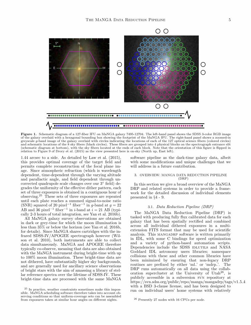
Figure 1. Schematic diagram of a 127-fiber IFU on MaNGA galaxy 7495-12704. The left-hand panel shows the SDSS 3-color RGB imageof the galaxy overlaid with a hexagonal bounding box showing the footprint of the MaNGA IFU. The right-hand panel shows a zoomed-ingreyscale g-band image of the galaxy overlaid with circles indicating the locations of each of the 127 optical science fibers (colored circles)and schematic locations of the 8 sky fibers (black circles). These fibers are grouped into 4 physical blocks on the spectrograph entrance slit(schematic diagram at bottom), with the sky fibers located at the ends of each block. Note that the orientation of this figure is flipped inrelation to Figure 9 of Drory et al. (2015) as the view presented here is on-sky (North up, East left).

1.44 arcsec to a side. As detailed by Law et al. (2015),this provides optimal coverage of the target field andpermits complete reconstruction of the focal plane im-age. Since atmospheric refraction (which is wavelengthdependent, time-dependent through the varying altitudeand parallactic angle, and field dependent through un-corrected quadrupole scale changes over our 3 field) de-grades the uniformity of the effective dither pattern, eachset of three exposures is obtained in a contiguous hour ofobserving.25 These sets of three exposures are repeateduntil each plate reaches a summed signal-to-noise ratio(SNR) squared of 20 pixel−1 fiber−1 in g-band at g = 22AB and 36 pixel−1 fiber−1 in i-band at i = 21 AB (typi-cally 2-3 hours of total integration, see Yan et al. 2016b).

All MaNGA galaxy survey observations are obtainedin dark or grey-time for which the moon illumination isless than 35% or below the horizon (see Yan et al. 2016b,for details). Since MaNGA shares cartridges with the in-frared SDSS-IV/APOGEE spectrograph however (Wil-son et al. 2010), both instruments are able to collectdata simultaneously. MaNGA and APOGEE thereforetypically co-observe, meaning that data are also obtainedwith the MaNGA instrument during bright-time with upto 100% moon illumination. These bright-time data arenot dithered, have substantially higher sky backgrounds,and are generally used for ancillary science observationsof bright stars with the aim of amassing a library of stel-lar reference spectra over the lifetime of SDSS-IV. Thesebright-time data are processed with the same MaNGA

25 In practice, weather constraints sometimes make this impos-sible. MaNGA scheduling software therefore takes into account ob-serving conditions so that uniform-coverage sets can be assembledfrom exposures taken at similar hour angles on different nights.

software pipeline as the dark-time galaxy data, albeitwith some modifications and unique challenges that wewill address in a future contribution.

3. OVERVIEW: MANGA DATA REDUCTION PIPELINE(DRP)

In this section we give a broad overview of the MaNGADRP and related systems in order to provide a frame-work for the detailed discussion of individual elementspresented in §4 - 9.

3.1. Data Reduction Pipeline (DRP)

The MaNGA Data Reduction Pipeline (DRP) istasked with producing fully flux calibrated data for eachgalaxy that has been spatially rectified and combinedacross all individual dithered exposures in a multi-extension FITS format that may be used for scientificanalysis. This mangadrp software is written primarilyin IDL, with some C bindings for speed optimizationand a variety of python-based automation scripts.Dependencies include the SDSS idlutils and NASAGoddard IDL astronomy users libraries; namespacecollisions with these and other common libraries havebeen minimized by ensuring that non-legacy DRProutines are prefixed by either ‘ml ’ or ‘mdrp ’. TheDRP runs automatically on all data using the collab-oration supercluster at the University of Utah26, ispublicly accessible in a subversion svn repository athttps://svn.sdss.org/public/repo/manga/mangadrp/tags/v1 5 4with a BSD 3-clause license, and has been designed torun on individual users’ home systems with relatively

26 Presently 27 nodes with 16 CPUs per node.

6 Law et al.

little overhead.27 Version control of the mangadrpcode and dependencies is done via svn repositoriesand traditional trunk/branch/tag methods; the versionof mangadrp described in the present contributioncorresponds to tag v1 5 4 for public release DR13. Wenote that v1 5 4 is nearly identical to v1 5 1 (which hasbeen used for SDSS-IV internal release MPL-4) save forminor improvements in cosmic ray rejection routinesand data quality assessment statistics.

The DRP consists of two primary parts: the 2d stagethat produces flux calibrated fiber spectra from individ-ual exposures, and the 3d stage that combines individ-ual exposures with astrometric information to producestacked data cubes. The overall organization of the DRPis illustrated in Figure 2. Each day when new dataare automatically transferred from APO to the SDSS-IV central computing facility at the University of Utah acronjob triggers automated scripts that run the 2d DRPon all new exposures from the previous modified Juliandate (MJD). These are processed on a per-plate basis,and consist of a mix of science and calibration exposures(flatfields and arcs).

The 2d stage of the MaNGA DRP is largely derivedfrom the BOSS idlspec2d pipeline (see, e.g., Dawson etal. 2013, Schlegel et al. in prep.)28 that has been modi-fied to address the different hardware design and sciencerequirements of the MaNGA survey (we summarize thenumerous differences in Appendix A). Each frame un-dergoes basic preprocessing to remove overscan regionsand variable-quadrant bias before the 1-d fiber spectraare extracted from the CCD detector image. The DRPfirst processes all of the calibration exposures to deter-mine the spatial trace of the fiber spectra on the detec-tor and extract fiber flatfield and wavelength calibrationvectors, and applies these to the corresponding scienceframes. The science exposures are in turn extracted,flatfielded, and wavelength calibrated using the corre-sponding calibration files. Using the sky fibers presentin each exposure we create a super-sampled model ofthe background sky spectrum, and subtract this off fromthe spectra of the individual science fibers. Finally, thetwelve minibundles targeting standard stars in each ex-posure are used to determine the flux calibration vectorfor the exposure compared to stellar templates. The finalproduct of the 2d stage is a single FITS file per exposure(mgCFrame) containing row-stacked spectra (RSS; i.e., atwo-dimensional array in which each row corresponds toan individual one-dimensional spectrum) of each of the1423 fibers interpolated to a common wavelength gridand combined across the four individual detectors.

Once a sufficient number of exposures have been ob-tained on a given plate, it is marked as complete at APOand a second automated script triggers the 3d stage DRPto combine each of the mgCFrame files resulting from the2d DRP. For each IFU (including calibration minibun-dles) on the plate, the 3d pipeline identifies the relevantspectra in the mgCFrame files and assembles them intoa master row-stacked format consisting of all spectra forthat target. The astrometric solution as a function of

27 Installation instructions are available athttps://svn.sdss.org/public/repo/manga/mangadrp/tags/v1 5 4/pdf/userguide.pdf

28 The idlspec2d software has also been used for the DEEP2survey; see Newman et al. (2013).

wavelength for each of these spectra is computed on aper-exposure basis using the known fiber bundle metrol-ogy and dither offset for each exposure, along with a va-riety of other factors including field and chromatic differ-ential refraction (see Law et al. 2015). This astrometricsolution is further refined using SDSS broadband imagingof each galaxy to adjust the position and rotation of theIFU fiber coordinates. Using this astrometric informa-tion the DRP combines the fiber spectra from individualexposures into a rectified data cube and associated in-verse variance and mask cubes. In post processing, theDRP additionally computes mock broadband griz im-ages derived from the IFU data, estimates of the recon-structed PSF at griz, and a variety of quality controlmetrics and reference information.

The final DRP data products in turn feed into theMaNGA Data Analysis Pipeline (DAP) which performsspectral modeling, kinematic fitting, and other analysesto produce science data products such as Hα velocitymaps, kinemetry, spectral emission line ratio maps, etc.from the data cubes. DAP data products will be madepublic in a future release and described in a forthcomingcontribution by Westfall et al. (in prep).

3.2. Quick-reduction pipeline (DOS)

Rather than running the full DRP in realtime at theobservatory, we instead use a pared-down version of thecode that has been optimized for speed that we refer toas DOS.29 The DOS pipeline shares much of its codewith the DRP, performing reduction of the calibrationand science exposures up through sky subtraction. Theprimary difference is in the spectral extraction; while theDRP performs an optimized profile fitting technique toextract the spectra of each fiber (see §4.2.2), DOS insteaduses a simple boxcar extraction that sacrifices some ac-curacy and robustness for substantial gains in speed.

The primary purpose of DOS is to provide real-timefeedback to APO observers on the quality and depth ofeach exposure. Each exposure is characterized by an ef-fective depth given by the mean SNR squared at a fixedfiber2mag 30 of 22 (g-band) and 21 (i-band). The SNR ofeach fiber is calculated empirically by DOS from the sky-subtracted continuum fluxes and inverse variances, whilenominal fiber2mags for each fiber in a galaxy IFU are cal-culated by applying aperture photometry to SDSS broad-band imaging data at the known locations of each of theIFU fibers (see §8.1) and correcting for Galactic fore-ground extinction following Schlegel et al. (1998). As il-lustrated in Figure 3, the SNR as a function of fiber2magfor all fibers in a given exposure forms a logarithmic re-lation that can be fitted and extrapolated to the effectiveachieved SNR at fixed nominal magnitudes g = 22 andi = 21. This calculation is done independently for allfour cameras using a g-band effective wavelength rangeλλ 4000-5000 A and an i-band effective wavelength rangeλλ6910−8500 A. As described above in §2.2, we integrateon each plate until the cumulative SNR2 in all complete

29 Daughter-of-Spectro. This pipeline is a sibling to the Son-of-Spectro quick reduction pipeline used by the BOSS and eBOSSsurveys, both of which are descended from the original SDSS-ISpectro pipeline.

30 Fiber2mag is a magnitude measuring the fluxcontained within a 2 arcsec diameter aperture; seehttp://www.sdss.org/dr13/algorithms/magnitudes/#mag fiber

The MaNGA Data Reduction Pipeline 7

MaNGA Pipeline

Data arrives from APO

MaNGA DRP 2d stage

MaNGA DRP 3d stage

Output Data Products

MaNGA DRP 2d Stage

runManga2d mdrp_reduce2d

mgArc-mgFlat-

mgFrame- mgSFrame- mgFFrame-

Preprocessing

Science Extraction Sky Subtraction Flux Calibration

Proceed to 3d Stage

Extraction

Wavelength Rectification

mgCFrame-

Calibration

MaNGA DRP 3d Stage

runManga3dPreimaging

Datamdrp_reduce3d mdrp_reduceoneifu

Astrometric Registration

Cube Constructionmanga-*-CUBEmanga-*-RSS

Proceed to MaNGA DAP

Pipeline

LegendInput To

Outputs

Data FITS Files

IDL Code

Pipeline Stage

Figure 2. Schematic overview of the MaNGA data reduction pipeline. The DRP is broken into two stages: mdrp reduce2d andmdrp reduce3d. The 2d pipeline data products are flux calibrated individual exposures corresponding to an entire plate; the 3d pipelineproducts are summary data cubes and row-stacked-spectra for a given galaxy combining information from many exposures.

Figure 3. SNR as a function of extinction-corrected fiber magni-tude for blue (left panel) and red cameras (right panel), for spectro-graphs 1 and 2 (diamond vs square symbols respectively). The redline indicates the logarithmic relation derived from fitting pointsin the magnitude range indicated by the vertical dotted lines. Thefilled red circle indicates the derived fit at the nominal magnitudesg = 22 and i = 21, with the SNR2 values given for each spec-trograph. This example corresponds to MaNGA plate 7443, MJD56741, exposure 177378.

sets of exposures reaches 20 pixel−1 fiber−1 in g-band and36 pixel−1 fiber−1 in i-band at the nominal magnitudesdefined above.

3.3. Metadata

MaNGA is a complex survey which requires trackingof multiple levels of metadata (e.g., fiber bundle metrol-ogy, cartridge layout, fiber plugging locations, etc.), anyof which may change on the timescale of a few days (in

the case of fiber plugging locations) to a few years (if car-tridges and/or fiber bundles are rebuilt). At any point,it must be possible to rerun any given version of thepipeline with the corresponding metadata appropriatefor the date of observations. This metadata must also beused throughout the different phases of the survey fromplanning and target selection, to plate drilling, to APOoperations, to eventual reduction and post-processing.

To this end, MaNGA maintains a central metadatarepository mangacore which is automatically synchro-nized between APO and the Utah data reduction hubusing daily crontabs. Version control of files within man-gacore is maintained by a combination of modified Ju-lian date (MJD) datestamps and periodic svn tags cor-responding to major data releases (v1 2 3 for DR13).

3.4. Quality Control

Given the volume of data that must be processedby the MaNGA pipeline (∼ 10 million reduced galaxyspectra and ∼ 100 million raw-frame spectra overthe six-year lifetime of SDSS-IV31), automated qual-ity control is essential. To that end, multiple mon-itoring routines are in place. The 2d and 3d stageDRP has bitmasks (MANGA DRP2PIXMASK andMANGA DRP3PIXMASK respectively) associated withthe primary flux extensions that can be used to indicate

31 Assuming an average of 3 clear hours per night between thebright and dark time programs, 5 exposures per hour (includingcalibrations), and ∼ 3000 spectra per exposure amongst 4 individ-ual CCDs.

8 Law et al.

individual pixels (or spaxels32 in the case of the 3d datacubes) that are identified as problematic. In the 2d case(spectra of all 1423 individual fibers within a single expo-sure), this pixel mask indicates such things as cosmic rayevents, bad flatfields, missing fibers, extraction problems,etc. In the 3d stage (a composite cube for a single galaxythat combines many individual exposures into a regular-ized grid), this pixel mask indicates things like low/nofiber coverage, foreground star contamination, and otherissues that mean a given spaxel should not be used forscience.

Additionally, there are overall quality bitsMANGA DRP2QUAL and MANGA DRP3QUALthat pertain to an entire exposure or data cube respec-tively and indicate potential issues during processing.In the 2d case, this can include effects like heavy cloudcover, missing IFUs, or abnormally high scatteredlight. In the 3d case, this can include warnings for badastrometry, bad flux calibration, or (rarely) a criticalproblem suggesting that a galaxy should not be usedfor science. As of DR13, 22 of the 1390 galaxy datacubes are flagged as critically problematic for a varietyof reasons ranging from the severe and unrecoverable(e.g., poor focus due to hardware failure, ∼ 5 objects)to the potentially recoverable in a future data release(e.g., failed astrometric registration due to a bright starat the edge of the IFU bundle) to the mundane (errantunflagged cosmic ray confusing the flux calibration QAroutine).

All of these pixel-level and exposure-level data qual-ity flags are used by the pipeline in deciding how andwhether to continue to process data (e.g., flux calibra-tion will not be attempted on an exposure flagged ascompletely cloudy). We provide a reference table of thekey MaNGA quality control bitmasks in Appendix B.4.

4. SPECTRAL EXTRACTION

MaNGA exposures are differentiated fromBOSS/eBOSS exposures taken with the same spec-trographs using FITS header keywords, and a planfile33

is created for each plate on a given MJD detailing eachof the exposures obtained for which the quality wasdeemed by DOS at APO to be excellent. The MaNGADRP parses this planfile and performs pre-processing,spectral extraction, flatfielding, wavelength calibration,sky subtraction, and flux calibration on a per-exposurebasis.

4.1. Preprocessing

Raw data from each of the four CCDs (b1, r1, b2, r2)are in the format of 16 bit images with 4352 columns and4224 rows (Table 3), with a 4096 x 4112 pixel active area(for the blue CCDs; 4114 × 4128 pixel active area forthe red CCDs) and overscan regions along each edge ofthe detector. As described by Dawson et al. (2013), theCCDs are read out with 4 amplifiers, one for each quad-rant, resulting in variable bias levels. Each exposure ispreprocessed to remove the overscan regions of the de-tector, subtract off quadrant-dependent biases, convert

32 Spatial picture element.33 A planfile is a plaintext ascii file that is both machine and hu-

man readable (see http://www.sdss.org/dr13/software/par/) andcontains a list of the science and calibration exposures to be pro-cessed through a given stage of the pipeline.

from bias corrected ADUs to electrons using quadrant-dependent gain factors derived from the overscan re-gions34, and divide by a flatfield containing the relativepixel-to-pixel response measured from a uniformly illu-minated calibration image (see Figure 4).

A corresponding inverse variance image is createdusing the measured read noise and photon counts ineach pixel; this inverse variance array is capped sothat no pixel has a reported SNR greater than 100.35

Finally, potential cosmic rays (which affect ∼ tentimes as many pixels in the red cameras as in theblue) are identified and flagged using the same algo-rithm adopted previously by the SDSS imaging andspectroscopic surveys. As discussed by R. H. Lup-ton (see http://www.astro.princeton.edu/∼rhl/photo-lite.pdf), this algorithm is a first-pass approach that suc-cessfully detects most cosmic rays by looking for fea-tures sharper than the known detector PSF but some-times incompletely flags pixels around the edge of cos-mic ray tracks. A second-pass approach that addressesthese residual features is applied later in the pipeline, asdescribed in §7. The inverse variance image is combinedwith this cosmic ray mask and a reference bad pixel maskso that affected pixels are assigned an inverse variance ofzero (and hence have zero weight in the reductions).

4.2. Calibration Frames

All flatfield and arc calibration frames from a plan-file are reduced prior to processing any science frames.These provide estimates of the fiber-to-fiber flatfield andthe wavelength solution, and are also critical for deter-mining the locations of individual fiber spectra on thedetectors. Since there are 4 cameras, each reduced flat-field (arc) exposure corresponds to four mgFlat (mgArc)multi-extension FITS files as described in the data modelin §B.

4.2.1. Spatial Fiber Tracing

As illustrated in Figure 4, MaNGA fibers are arrangedinto blocks of 21-39 fibers with 22 blocks on each spectro-graph, with individual spectra running vertically alongeach CCD. The fiber spacing within blocks is 177 µm forscience IFUs (∼ 4 pixels), and 204 µm for spectropho-tometric calibration IFUs, with ∼ 624 µm between eachblock. Fibers are initially identified in a uniformly illu-minated flat field image using a cross-correlation tech-nique to match the 1d profile along the middle row ofthe detector against a reference file describing the nom-inal location of each fiber in relative pixel units. Thecross correlation technique matching against all fibers ona given slit allows for shifts due to flexure-based opticaldistortions while ensuring robustness against missing orbroken individual fibers and/or entire IFUs. Fibers thatare missing within the central row are flagged as dead inmangacore .

With the initial x-positions of each fiber in the cen-tral row thus determined, the centroids of each fiber in

34 Typical read noise and detector gains are given in Table 3;these are slightly different for each quadrant of each detector, andcan evolve over the lifetime of the survey. See Smee et al. (2013)for details.

35 This helps resolve problems arising when extracting extremelybright spectral emission lines.

The MaNGA Data Reduction Pipeline 9

FiberID

Wa

ve

len

gth

Calibration minibundlesA B

C

Figure 4. Illustration of the MaNGA raw data format before (A) and after (B) preprocessing to remove the overscan and quadrant-dependent bias. This image shows a color-inverted typical 15-minute science exposure for the b1 camera (exposure 177378 for plate 7443on MJD 56741). There are 709 individual fiber spectra on this detector, grouped into 22 blocks. Bright spectra represent central regionsof the target galaxies and/or spectrophotometric calibration stars; bright horizontal features are night-sky emission lines. Panel C zoomsin on 10 blocks in the wavelength regime of the bright [O I 5577] skyline.

the other rows are then determined using a flux-weightedmean with a radius of 2 pixels. This algorithm sequen-tially steps up and down the detector from the centralrow, using the previous row’s position as the initial in-put to the flux-weighted mean. Fibers with problem-atic centroids (e.g. due to cosmic rays) are masked out,and replaced with estimates based on neighboring traces.These flux-weighted centroids are further refined using aper-fiber cross-correlation technique matching a gaussianmodel fiber profile (see §4.2.2) against the measured pro-file in a given row. This fine adjustment is required inorder to remove sinusoidal variations in the flux-weightedcentroids at the∼ 0.1 pixel level caused by discrete jumpsin the pixels included in the previous flux-weighted cen-troiding.

Once the positions of all fibers across all rows of thedetector have been computed, the discrete pixel locationsare stored as a traceset36 of 7th order Legendre polyno-

36 A traceset is a set of coefficient vectors defining functionsover a common independent-variable domain specified by ‘xmin’and ‘xmax’ values. The functions in the set are defined in terms of

mial coefficients. An iterative rejection method accountsfor scatter and uncertainty in the centroid measurementof individual rows and ensures realistically smooth vari-ation of a given fiber trace as a function of wavelengthalong the detector. The best-fit traceset coefficients arestored as an extension in the per-camera mgFlat files(Table B2).

4.2.2. Spectral Extraction

Similarly to the BOSS survey (Dawson et al. 2013),we extract individual fiber spectra from the 2d detectorimages using a row-by-row optimal extraction algorithmthat uses a least-squares profile fit to obtain an unbiasedestimate of the total counts (Horne 1986). The counts in

a linear combination of basis functions (such as Legendre or Cheby-shev polynomials) up to a specified maximum order, weighted bythe values in the coefficient vectors, and evaluated using a suitableaffine rescaling of the dependent-variable domain (such as [xmin,xmax] → [-1, 1] for Legendre polynomials). For evaluation pur-poses, the domain is assumed by default to be a zero-based integerbaseline from xmin to xmax such as would correspond to a digitaldetector pixel grid.

10 Law et al.

each row are modeled by a linear combination of Nfiber37

Gaussian profiles plus a low-order polynomial (or cubicbasis-spline; see §4.2.3) background term. As we illus-trate in Fig. 5 (right panel), the resulting model is anextremely good fit to the observed profile. MaNGA usesthe extract row.c code (dating back to the original SDSSspectroscopic survey) which creates a pixelwise model ofthe gaussian profile integrated over fractional pixel posi-tions (i.e. the profile is assumed to be gaussian prior topixel convolution), describes deviations to the line cen-ters and widths as linear basis modes (representing thefirst and second spatial derivatives, respectively), andsolves for the banded matrix inversion by Cholesky de-composition. An initial fit to the flatfield calibrationimages allows both the amplitude and the width of theGaussian profiles in each row to vary freely, with the cen-troid set to the positions determined via fiber tracing in§4.2.1. These individual width measurements are noisyhowever, and for each block of fibers we therefore fit thederived widths with a linear relation as a function offiberid along the slit in order to reject errant values anddetermine a fixed set of fiber widths that vary smoothly(within a given block) with both fiberid and wavelength.As illustrated in Figure 6, low-frequency variation of thewidths with fiberid reflects the telescope focus (which wechoose to ensure that the widths are as constant as pos-sible across the entire slit), while discontinuities at theblock boundaries are due to slight differences in the slit-head mounting. These fixed widths are then used in asecond fit to the detector images in which only the poly-nomial background and the amplitude of the Gaussianterms are allowed to vary.

The final value adopted for the total flux in each rowis the integral of the theoretical gaussian profile fits tothe observed pixel values, while the inverse variance istaken to be the diagonal of the covariance matrix fromthe Cholesky decomposition. This approach allows usto be robust against cosmic rays or other detector ar-tifacts that cover some fraction of the spectrum, sinceunmasked pixels in the cross-dispersion profile can stillbe used to model the Gaussian profile (Figure 5). Ad-ditionally, this technique naturally allows us to modeland subtract crosstalk arising from the wings of a givenprofile overlapping any adjacent fibers, and to estimatethe variance on the extracted spectra at each wavelength.This step transforms our 4096 × 4112 CCD images (4114× 4128 for the red cameras) to row-stacked spectra withdimensionality 4112 ×Nfiber (4128 ×Nfiber for the redcameras)

4.2.3. Scattered Light

The DRP automatically assesses the level of scatteredlight in the MaNGA data by taking advantage of thehardware design in which gaps of ∼ 16 pixels were left be-tween each v-groove block (compared to ∼ 4 pixels peak-to-peak between each fiber trace within a block) so thatthe interstitial regions contain negligible light from thegaussian fiber profile cores (Drory et al. 2015). By mask-ing out everything within 5 pixels of the fiber traces wecan identify those pixels on the edge of the detector andin empty regions between individual blocks whose counts

37 Nfiber is the number of fibers on a given detector (Nfiber = 709for spectrograph 1, Nfiber = 714 for spectrograph 2).

are dominated by diffuse light on the detector. This lightis a combination of 1) genuine scattered light that entersthe detector via multiple reflections from unbaffled sur-faces and 2) highly-extended non-gaussian wings to theindividual fiber profiles that can extend to hundreds ofpixels and contain ∼ 1− 2% of the total light of a givenfiber.

For MaNGA dark-time science exposures (which typ-ically peak at about 30 counts pixel−1 fiber−1 for thesky continuum) both components are small and can besatisfactorily modeled by a low-order polynomial term ineach extracted row. For some bright-time exposures usedin the stellar library program however, the moon illumi-nation can approach 100% and produce larger scatteredlight counts∼ a quarter of the sky background seen by in-dividual fibers. Additionally, for our flat-field calibrationexposures the summed contribution of the non-gaussianwings to the fiber profiles can reach ∼ 300 counts pixel−1

in the interstial regions between blocks (compared to∼ 20, 000 counts pixel−1 in the fiber profile cores). Inboth cases the simple polynomial background term canprove unsatisfactory, and we instead fit the counts in theinterstitial regions row-by-row with a fourth-order ba-sis spline model that allows for a greater degree of spa-tial variability in the background than is warranted forthe dark-time science exposures. This bspline model isevaluated at the locations of each intermediate pixel andsmoothed along the detector columns by use of a 10-pixelmoving boxcar to mitigate the impact of individual badpixels. The resulting bspline scattered light model is sub-tracted from the raw counts before performing spectralextraction.

4.2.4. Fiber Flatfield

Each flatfield calibration frame is extracted into in-dividual fiber spectra using the above techniques andmatched to the nearest (in time) arc-lamp calibrationframe which has been processed as described in §4.2.5.Using the wavelength solutions derived from the arcframes, we combine the individual flatfield spectra (firstnormalized to a median of unity) into a single compos-ite spectrum with substantially greater spectral samplingthan any individual fiber.38 We fit this composite spec-trum with a cubic basis spline function to obtain thesuperflat vector describing the global flatfield response(i.e., the quartz lamp spectrum convolved with the de-tector response and system throughput). This global su-perflat is shown in Figure 7, and illustrates the falloff insystem throughput toward the wavelength extremes ofthe detector (see also Fig. 4 of Yan et al. 2016a).

We evaluate the superflat spline function on the na-tive wavelength grid of each individual fiber and divideit out from the individual fiber spectra in order to ob-tain the relative fiber-to-fiber flatfield spectra. So nor-malized, these fiber-to-fiber flatfield spectra have valuesnear unity, vary only slowly (if at all) with wavelength,and easily show any overall throughput differences be-tween the individual fibers. Each such spectrum is inturn fitted with a bspline in order to minimize the con-tribution of photon noise to the resulting fiber flats andinterpolate across bad pixels. In the end, we are left with

38 Since each fiber has a slightly different wavelength solutionwe effectively supersample the intrinsic input spectrum.

The MaNGA Data Reduction Pipeline 11

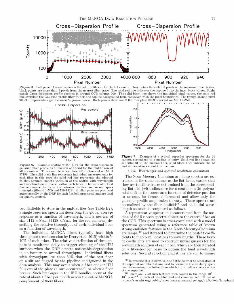
Figure 5. Left panel: Cross-dispersion flatfield profile cut for the R1 camera. Grey points lie within 5 pixels of the measured fiber traces,black points are more than 5 pixels from the nearest fiber trace. The solid red line indicates the bspline fit to the inter-block values. Rightpanel: Cross-dispersion profile zoomed in around CCD column 900. The solid black line shows the individual pixel values, the solid redline overplots the Gaussian profile fiber fit plus the bspline background term convolved with the pixel boundaries. The trough around pixel900-910 represents a gap between V-groove blocks. Both panels show row 2000 from plate 8069 observed on MJD 57278.

Figure 6. Example spatial width (1σ) for the cross-dispersiongaussian fiber profile as a function of fiberid for the middle row ofall 4 cameras. This example is for plate 8618, observed on MJD57199. The solid black line represents individual measurements foreach fiber in this row; the solid red line represents the adoptedfit that assumes smooth variation of the widths with wavelengthand as a function of fiberid within each block. The vertical dottedline represents the transition between the first and second spec-trographs (fiberid 1-709 and 710-1423). Similar plots are producedautomatically by the DRP for each flatfield processed, and are usedfor quality control.

two flatfields to store in the mgFlat files (see Table B2);a single superflat spectrum describing the global averageresponse as a function of wavelength, and a fiberflat ofsize 4112 ×Nfiber (4128 ×Nfiber for the red cameras) de-scribing the relative throughput of each individual fiberas a function of wavelength.

The individual MaNGA fibers typically have highthroughput (see discussion by Drory et al. 2015) within 5-10% of each other. The relative distribution of through-puts is monitored daily to trigger cleaning of the IFUsurfaces when the DRP detects noticeable degradationin uniformity or overall throughput. Individual fiberswith throughput less than 50% that of the best fiberon a slit are flagged by the pipeline and ignored in thedata analysis. This may occur when a fiber and/or IFUfalls out of the plate (a rare occurrence), or when a fiberbreaks. Such breakages in the IFU bundles occur at therate of about 1 fiber per month across the entire MaNGAcomplement of 8539 fibers.

3500 4000 4500 5000 5500 6000λ (Angstroms)

0.0

0.5

1.0

1.5

2.0

No

rma

lize

d flu

x

Figure 7. Example of a typical superflat spectrum for the b1camera normalized to a median of unity. Solid red line shows thesuperflat fit to the median fiber, solid black lines indicate the 1σand 2σ deviations about this median.

4.2.5. Wavelength and spectral resolution calibration

The Neon-Mercury-Cadmium arc-lamp spectra are ex-tracted in the same manner as the flat-fields, except thatthey use the fiber traces determined from the correspond-ing flatfield (with allowance for a continuous 2d polyno-mial shift in the traces as a function of detector positionto account for flexure differences) and allow only thegaussian profile amplitudes to vary. These spectra arenormalized by the fiber flatfield39 and an initial wave-length solution is computed as follows.

A representative spectrum is constructed from the me-dian of the 5 closest spectra closest to the central fiber onthe CCD. This spectrum is cross-correlated with a modelspectrum generated using a reference table of knownstrong emission features in the Neon-Mercury-Cadmiumarc lamps,40 and iterated to determine the best-fit coeffi-cients to map pixel locations to wavelengths. These best-fit coefficients are used to contruct initial guesses for thewavelength solution of each fiber, which are then iteratedon a fiber-to-fiber basis to obtain the final wavelengthsolutions. Several rejection algorithms are run to ensure

39 In practice this is iterative; the flatfields prior to separation ofthe superflat and fiberflat are used to normalize the arc-lamp spec-tra, the wavelength solution from which in turn allows constructionof the superflat.

40 There are ∼ 50 such features with counts in the range 103 –105 pixel−1 in each of the blue and red cameras; see full list athttps://svn.sdss.org/public/repo/manga/mangadrp/tags/v1 5 4/etc/lamphgcdne.dat

12 Law et al.

Spectral Line-Spread Function

Figure 8. As Figure 6, but showing the spectral line spread func-tion (1σ LSF) for the gaussian arcline profile as a function of fiberidfor an emission line near the middle row of all 4 detectors (Cd I5085.822 A for the blue cameras, Ne I 8591.2583 A for the redcameras).

reliable arc-line centroids across all fibers. A final 6thorder Legendre polynomial fit converts the wavelengthsolutions into a series of polynomial traceset coefficients.The higher order coefficients are forced to vary smoothlyas a function of fiberid since they predominantly arisefrom optical distortions along the slit (whereas lowerorder terms represent differences arising from the fiberalignment). These coefficients are stored as an exten-sion in the output mgArc file (see Table B1), and usedto reconstruct the wavelength solutions at all fibers andpositions on the CCD.

The arc-lamp spectral resolution (hereafter the linespread function, or LSF) is computed by fitting the ex-tracted spectra around the strong arc lamp emission linesin each fiber with a Gaussian profile integrated overeach pixel (note that we integrate the fitted profile shapeacross each pixel rather than simply evaluating the pro-file at the pixel midpoints; see discussion in §10.2) andallowing both the width and amplitude of the profile tovary. As illustrated in Figure 8, these widths are intrin-sically noisy and the DRP therefore fits them with a lin-ear relation as a function of fiberid along the slit in orderto reject errant values and determine a fixed set of linewidths that vary smoothly (within a given block) withfiberid. These arcline widths are then fit with a Leg-endre polynomial traceset that is stored in the mgArcfiles and evaluated at each pixel to compute the LSF atwavelengths between the bright arc lines.

Both wavelength and LSF solutions derived from thearc frames are later adjusted for each individual scienceframe to account for instrumental flexure during and be-tween (see discussion in §4.3).

All calibrations are additionally complicated in the redcameras since the middle row of pixels on these detectorsis oversized by a factor of 1/3, causing a discontinuityin both the wavelength solution and the LSF for eachfiber as a function of pixel number. All of the algorithmsdescribed above therefore allow for such a discontinuityacross the CCD quadrant boundary. The primary im-pact of this discontinuity on the final data products is toproduce a spike of low spectral resolution around 8100A, the exact wavelength of which can vary from fiber tofiber based on the curvature of the wavelength solutionalong the detector.

4.3. Science Frames

Each science frame is associated with the arc and flatpair taken closest to it in time (generally within one hoursince calibration frames are taken at the start of eachplate and periodically thereafter), and extracted row-by-row following the method outlined in §4.2.2. During thisextraction only the profile amplitudes and backgroundpolynomial term are allowed to vary freely; the tracecentroids are tied to the flatfield traces with a global 2dpolynomial shift to account for instrument flexure, andthe cross-dispersion widths are fixed to the values derivedfrom the flatfield. The extracted spectra are normalizedby the superflat and fiber flat vectors derived from theflatfield.

The wavelength solutions derived from the arcs are ad-justed for each science frame to match the known wave-lengths of bright night-sky emission lines in the sciencespectra by fitting a low-order polynomial shift as a func-tion of detector position to allow for instrumental flex-ure (these shifts are typically less than a quarter pixel).The final wavelength solution for each exposure is cor-rected to the vacuum heliocentric restframe using headerkeywords recording atmospheric conditions and the timeand date of a given pointing. As we explore in §10.3, weachieve a ∼ 10 km s−1 or better rms wavelength calibra-tion accuracy with zero systematic offset to within 2 kms−1.

Similarly, in order to account for flexure and vary-ing spectrograph focus with time the spectral LSF mea-surements derived from the arc-lamp exposures are alsoadjusted for each science frame to match the LSF ofbright skylines that are known to be unblended in high-resolution spectra (e.g., Osterbrock et al. 1996). Start-ing from the original arcline LSF model, we derive aquadrature correction term for the profile widths Q2 =σsky

2 − σarc2. Q is taken to be constant as a func-

tion of wavelength for each camera, and is based on thestrong auroral O I 5577 line in the blue (since the HgI lines are too weak and broadened to obtain a reliablefit) and an average of many isolated bright lines in thered.41 The measured quadrature correction term is fit-ted with a cubic basis spline to ensure that the correc-tion applied varies smoothly with fiberid. Across the ∼1100 individual exposures in DR13 the average correc-tion Q2 = 0.08 ± 0.04 pixel2 in the blue cameras andQ2 = 0.05± 0.02 pixel2 in the red cameras (likely due tothe flatter and more stable focus in the red cameras).

The final row-stacked spectra, inverse variances, pixelmasks, wavelength solutions, and broadened LSF are allstored as extensions in the output mgFrame FITS file(Table B3).

5. SKY SUBTRACTION

Unlike previous SDSS spectroscopic surveys targetingbright central regions of galaxies, MaNGA will exploreout to ≥ 2.5 effective radii (Re) where galaxy flux is de-creasing rapidly relative to the sky background. As illus-trated in Figure 9, this night sky background is especiallybright at near-IR wavelengths longwards of ∼ 8000 A,where bright emission lines from OH radicals (e.g., Rous-selot et al. 2000) dominate the background flux. These

41 See https://svn.sdss.org/public/repo/manga/mangadrp/tags/v1 5 4/etc/skylines.datfor a complete list.

The MaNGA Data Reduction Pipeline 13

OH features vary in strength with both time and angularposition depending on the coherence scale of the atmo-sphere, posing challenges for measuring faint stellar at-mospheric features such as the Wing-Ford (Wing & Ford1969) band of iron hydride absorption lines around 9900A. In many cases such faint features will be detectableonly in stacked bins of spectra, driving the need to reachthe Poisson-limited noise regime so that stacked spectraare not limited by systematic sky subtraction residuals.

We therefore design our approach to sky subtractionwith the aim of reaching Poisson-limited performance atall wavelengths from λλ4000− 10, 000 A (beyond whichthe increasing read noise of the BOSS cameras prohibitssuch performance). Our sky subtraction algorithm isclosely based on the routines developed for the BOSS sur-vey, and relies on using the dedicated 92 sky fibers (46per spectrograph) on each plate to construct a highly-sampled model background sky that can be subtractedfrom each of the science fibers. These sky fibers areplugged into regions identified during the plate designprocess as blank sky ‘objects’ within a 14 arcmin patrolradius of their associated IFU fiber bundle (see Fig. 1).

5.1. Sky Subtraction Procedure

Sky subtraction is performed independently for each ofthe 4 cameras using the flatfielded, wavelength-calibratedfiber spectra contained in the mgFrame files, and is amulti-step iterative process. Broadly speaking, we builda super-sampled sky model from all of the sky fibers,scale it to the sky background level of a given block, andevaluate it on the native solution of each fiber withinthat block. In detail:

1. The metadata associated with the exposure is usedto identify the Nsky individual sky fibers in eachframe based on their FIBERTYPE.

2. Pixel values for these Nsky sky fibers are resortedas a function of wavelength into a single one-dimensional array of length Nsky × Nspec (whereNspec is the length of a single spectrum). Since eachfiber has a unique wavelength solution, this super-sky vector has much higher effective sampling ofthe night sky background spectrum than any indi-vidual fiber and provides an accurate line spreadfunction (LSF) for OH airglow features. An exam-ple of this procedure is shown in Figure 10.

3. Similarly, we also construct a super-sampled weightvector by comining individual sky fiber inversevariance spectra that have first been smoothed bya boxcar of width 100 pixels (∼ 100−200 A) in thecontinuum and 2 pixels (∼ 2− 3 A) within 3 A ofbright atmospheric emission features.

4. The super-sky spectrum is then weighted by thesmoothed inverse variance spectrum (convolvedwith the bad-pixel mask) and fitted with a cu-bic basis-spline as a function of wavelength, withthe number of breakpoints set to ∼ Nspec so thathigh-frequency variations (due, e.g., to shot noiseor bad pixels) are not picked up by the resulting

model (see, e.g., green line in Figure 10).42 Thebreakpoint spacing is set automatically to maintainapproximately constant S/N ratio between break-points. The B-spline fit itself is iterative, with up-per and lower rejection threshholds set to maskbad or deviant pixels. We note that the smoothingof the inverse variance in determining the weightfunction is critical as otherwise the weights (whichare themselves estimated from the data) would mod-ulate with the Poisson scatter and bias the fit to-wards slightly lower values, resulting in systematicundersubtraction of the sky background, especiallynear the wavelength extrema where the overall sys-tem throughput is low.

5. This B-spline function is evaluated on the nativewavelength solution of each of the sky fibers. Di-viding the original sky fiber spectra by this func-tional model, and collapsing over wavelengths us-ing a simple mean we arrive at a series of scale fac-tors describing the relative sky background seen bythe fiber compared to all other fibers on the detec-tor. For each harness (i.e., each IFU plus associatedsky fibers) we compute the median of these scalefactors to obtain a single averaged scale factor foreach harness. These scale factors help account fornearly-grey variations in the true sky continuumacross our large field produced by a combination ofintrinsic background variations and patchy cloud-cover. The variability in sky background betweenharnesses is about 1.5% rms, with some larger devi-ations > 5% observed during the bright time stellarlibrary program when pointing near a full moon canproduce strong background gradients.

6. Repeat steps 2-4 after first scaling each individualsky fiber spectrum by the value appropriate for itsharness in order to obtain a super-sky spectrumin which per-harness scaling effects have been re-moved.

7. Evaluate the new B-spline function on the nativepixellized wavelength solution of each fiber (skyplus science), and multiply it by the scaling fac-tor for the harness to obtain the first-pass modelsky spectrum for each fiber. Subtract this fromthe spectra to obtain the first pass sky subtractedspectra.

8. Identify deviant sky fibers in which the median sky-subtracted residual SNR2 > 2 (this is extremelyrare, and generally corresponds to a case where asky fiber location was chosen poorly, or a fiber wasmisplugged and not corrected before observing).Eliminate these sky fibers from consideration, andrepeat steps 2-7 to obtain the second-pass modelsky spectrum for each fiber. We refer to this as the1-d sky model.

9. Repeat steps 2-4, this time allowing the bsplinefit to accommodate a smoothly varying 3rd order

42 The number of breakpoints is reduced slightly in the bluecameras as there are few narrow spectral features that need to befit.

14 Law et al.

OH Skylines

[O I

55

77

]

HPS

Hg I

H+K

O2

Figure 9. Typical flux-calibrated MaNGA night-sky background spectrum seen by a single optical fiber (2 arcsec core diameter). Brightfeatures longward of 7000 A represent blended OH and O2 skyline emission (see, e.g., Osterbrock et al. 1996). The bright feature at 5577A is atmospheric [O I], the broad feature around 6000 A is high-pressure sodium (HPS) from streetlamps; Hg I from mercury vapor lampscontributes most of the discrete features at short wavelengths (see, e.g., Massey & Foltz 2000). Absorption features around 4000 A arezodiacal Fraunhofer H and K lines.

Figure 10. Example MaNGA super-sky spectrum created by thewavelength-sorted combination of all sky fiber spectra (black line)in the OH-emission dominated wavelength region λλ7900 − 7960A. Overlaid in green is the b-spline model fit to the super-skyspectrum; red points represent the b-spline model after evaluationon the native pixellized wavelength solution of a single fiber.

polynomial of values at each breakpoint as a func-tion of fiberid (i.e., rather than requiring the modelto be constant for all fibers, it is allowed to varyslowly as a function of slit position). This polyno-mial term is introduced in order to model variationsin the LSF along each slit; empirically, increasingpolynomial orders up to 3 results in an improve-ment of the skyline residuals, while no further gainsare observed at greater than 3rd order. Evaluatethe new B-spline function on the native pixellizedwavelength solution of each fiber (sky plus science)to obtain the 2-d sky model. Notably, this 2-d model does not use the explicit scaling used bythe 1-d model. This is partially because a similardegree of freedom is introduced by the 2d polyno-

mial, and partially because OH features can varyin strength independently from the underlying con-tinuum background (see, e.g., Davies 2007).

10. The final sky model is a piecewise hybrid of the1-d and 2-d models; in continuum regions it is takento be the 1-d model, and in the skyline regions (i.e.,within 3 A of any wavelength for which the skybackground is > 5σ above a bspline fit to the in-terline continuum) it is taken to be the 2-d model.We opt for this hybrid model as it optimizes ourvarious performance metrics: In the continuum farfrom night sky lines, our performance is limited bythe poisson-based RMS of the model sky spectrumsubtracted from each science fiber. Therefore, weuse the 1d model that is based on all 46 sky fiberson a given spectrograph. In contrast, near brightskylines our performance is instead limited by ourability to accurately model the shape of the sky-line wings, which can vary along the slit (see, e.g.,Fig 8). Therefore, in skyline regions we use the 2dmodel which improves the model LSF fidelity atthe expense of some SNR. There is no measurablediscontinuity between the sky-subtracted spectraat the piecewise 1d/2d model boundaries.

The final sky model is subtracted from the mgFramespectra; these sky-subtracted spectra are stored in mgS-Frame files (Table B4), which contain the spectra, in-verse variances (with appropriate error propagation),pixel masks, applied sky models, etc. in a row-stackedformat identical to the input mgFrame files.

5.2. Sky Subtraction Performance: All-Sky Plates

We estimate the accuracy of our calibration and skysubtraction up to this point by using specially designed

The MaNGA Data Reduction Pipeline 15

“all-sky” plates in which every science IFU is placed ona region of sky determined to be empty of visible sourcesaccording to the SDSS imaging data (calibration mini-bundles are still placed on standard stars so that theseall-sky plates can be properly flux calibrated). The re-sulting sky-subtracted sky spectra can then be used toestimate the accuracy of our noise model, extraction al-gorithms, and sky-subtraction technique.

Working with the row-stacked mgSFrame spectra (i.e.,prior to flux calibration and wavelength rectification) weconstruct ‘Poisson ratio’ images for each camera by mul-tiplying the sky-subtracted residual counts by the squareroot of the inverse variance (which accounts for both shotnoise and detector read noise). If the sky-subtraction isperfect, and the noise model properly estimated, thesepoisson ratio images should be devoid of structure witha Gaussian distribution of values with mean of 0 andσ = 1.0. In Figure 11 (right-hand panels) we show theactual distribution of values for the sky-subtracted sci-ence fibers for exposure 183643 (cart 4, plate 8069, MJD56901) for each of the four cameras (solid black lines)compared to the ideal theoretical expectations (solid redline; note that this is not a fit to the data). We findthat the overall distribution of values is broadly consis-tent with theoretical models in all four cameras (c.f. Fig23 of Newman et al. 2013, which shows similar plots forthe DEEP2 survey), albeit with some evidence for slightoversubtraction on average and a non-gaussian wing inthe blue cameras (pixels in this asymmetric wing do notcorrespond to particular wavelengths or fiberid).

We examine this behavior as a function of wavelengthin Figure 11 (left-hand panel) by plotting the 1σ widthof the gaussian that best fits the distribution of un-flagged pixel values at a given wavelength across all sci-ence fibers.43 As before, perfectly noise-limited sky sub-traction with a perfect noise model would correspond toa flat distribution of σ around 1.0 at all wavelengths; wenote that the blue cameras and the continuum regionsof the r2 camera are close to this level of performancewith up to a 3% offset from nominal (suggesting thatthe read noise in some quadrants may be marginally un-derestimated). In the r1 camera the read noise may beoverestimated by ∼ 10% in some quadrants (as σ < 1for r1 in the wavelength range λλ5700 − 7600 A), butis otherwise well-behaved in the continuum region. Inthe skyline regions of the red cameras, performance iswithin 10% of Poisson expectations out to ∼ 8500 A.Longward of ∼ 8500 A (where skylines are brighter, andthe spectra have greater curvature on the detectors) skysubtraction performance in skyline regions is ∼ 10 − 20% above theoretical expectations. This is likely due tosystematic residuals in the subtraction caused by block-to-block variations in the spectral LSF that are difficultto model completely. Indeed, such an analysis duringcommissioning revealed the OH skyline residuals weresignificantly worse in R1 than in the R2 camera. This ledto the discovery of optical coma in R1 that was fixed dur-ing Summer 2014 prior to the formal start of SDSS-IV,but which nonetheless affected the commissioning plates

43 Since each fiber has a different wavelength solution we can’tsimply use all pixels in a given column, and therefore instead usethe three pixels whose wavelengths are closest to a given wavelengthin each fiber.

7443 and 7495.Overall, the results in Figure 11 indicate excellent per-

formance from the MaNGA DR13 data pipeline sky sub-traction, albeit with some room for further improvementin future data releases. Finally, we assess whether anysystematics exist within the data that would prohibitstacking of multiple fiber spectra in order to reach faintsurface brightness levels (e.g., in the outer regions ofthe target galaxies). Using the flux-calibrated, camera-combined mgCFrame data (again corresponding to expo-sure 183643 from MJD 56901) we compute the limiting1σ surface brightness reached in the largely skyline-freewavelength range 4000 − 5500 A as a function of thenumber of individual fiber spectra stacked. As shownin Figure 12, when N fibers are stacked randomly fromacross both spectrographs (solid black line) the limiting

surface brightness decreases as√N−1 + 92−1 (i.e., im-

proving as√N for small N , and becoming limited by

the statistics of the 92-fiber sky model as N becomeslarge). If fibers are stacked sequentially along the slit(dashed black line) the limiting surface brightness de-

creases as√N−1 + 46−1 at first (since only the 46 sky

fibers on a single slit are being used in the sky model) butapproaches nominal performance again once fibers fromboth spectrographs are included in the stack (N > 621).

5.3. Sky Subtraction Performance: Skycorr

Another way to check the sky subtraction quality of theDRP is to compare its performance for a typical galaxyplate against the results obtained using the skycorr tool(Noll et al. 2014). Skycorr was designed as a data reduc-tion tool to remove sky emission lines for astronomicalspectra using physically motivated scaling relations, andhas been found to consistently perform better than thepopular algorithm of Davies (2007). As input, skycorrneeds the science spectrum and a sky spectrum, prefer-ably taken around the time as the science spectrum. Af-ter subtracting the continuum from both spectra, it thenscales the sky emission lines from the sky spectrum to fitthese lines in the science spectrum by comparing groupsof sky lines which should vary in similar ways.

In Figure 13 we compare a typical sky-subtractedMaNGA science spectrum obtained using the DRP al-gorithms described in §5 with the spectrum obtained us-ing skycorr instead. The two sky-subtracted spectra arenearly indistinguishable, indicating comparable perfor-mance between the two techniques.

6. FLUX CALIBRATION

Flux calibration for MaNGA (Yan et al. 2016a) hasa different goal than in previous generations of SDSSspectroscopic fiber surveys. The goal for single fiber fluxcalibration is often to retrieve the total flux of a point-likesource, accounting for both flux lost due to atmosphericattenuation (or instrumental response) and the flux lostdue to the fraction of the point-spread function that fallsoutside the fiber aperture. In contrast, IFU observationsprovide a sampling of the seeing-convolved flux profile forwhich we do not desire to make any aperture correctionsand must therefore seperate the aperture loss factor fromthe system response loss factor.

To achieve this goal, we allocate a set of twelve 7-fibermini-ifu bundles to standard stars on every plate (6 per

16 Law et al.

Spectrograph 1

Spectrograph 2

Figure 11. Left-hand panel: Actual noise in sky-subtracted spectra (from all-sky plate 8069, observed on MJD 56901) divided by thatexpected based on detector read noise and Poisson counting statistics as a function of wavelength for each spectrograph. The overlappingregion from λλ5900 − 6300 A is the dichroic region over which blue and red cameras are combined. The solid red line indicates unity; ifsky subtraction was done perfectly (and the noise properties of the spectra were estimated correctly) the black lines should nearly followthe red line at all wavelengths. Right-hand panel: Distribution of noise values divided by the expected for all 4 cameras (B1/B2/R1/R2).Black curves represent the measured distribution of values (3621-6300 A for B1 and B2, 5900-10354 A for R1 and R2), red curves representthe Gaussian ideal distribution with width Nσ = 1. Vertical dashed black lines represent the 1σ range.

μ

Figure 12. 1σ limiting surface brightness reached in the wave-length range λλ4000 − 5500 A in a single 15-minute exposure bya composite spectrum stacking N sky-subtracted science fibers(based on all-sky plate 8069, observed on MJD 56901). The solidblack line indicates results from stacking N science fibers selectedrandomly from across both spectrographs; this is extremely wellreproduced by the theoretical curve (solid red line) representing

expected performance based on√N−1 + 92−1. The dashed black

line indicates results from stacking N science fibers as a functionof fiberid along the spectrograph slit; this improves more slowly atfirst as

√N−1 + 46−1 (red dashed line).

spectrograph). Using the guider system to provide afirst-order estimate for the seeing profile in a given expo-sure we construct a model PSF as seen by each IFU mini-bundle by including the effects of wavelength-dependentseeing and the shape mismatch between the focal planeand the plate. This allows us to estimate the relativefluxes amongst the seven IFU fibers in several wavelengthwindows and fit for the spatial location of the star withinthe IFU, the scale of the PSF, and the scale and rotationof the expected differential atmosphere refraction (see§8.1). With the best fit PSF model, we can compute theaperture loss factor of the fibers and estimate the total

Figure 13. Example spectrum of a randomly chosen MaNGAfiber from a typical galaxy plate (plate 7443, MJD 56745, exposure177685) in the vicinity of an OH airglow region. The black line rep-resents the as-observed galaxy + sky spectrum, the dashed red linethe science spectrum after sky subtraction using the MaNGA DRP,and the blue line the science spectrum using instead the skycorr(Noll et al. 2014) algorithm. The two methods of sky subtrac-tion produce nearly identical results to within the DRP-estimateuncertainty (green line).

flux that would have been observed for each standardstar if the IFU had captured 100% of its light.

Given this aperture correction, we can then derive thesystem response as a function of wavelength in a similarway as BOSS (Dawson et al. 2013) by selecting the bestfitting template from a grid of theoretical spectra normal-ized to the observed SDSS broadband magnitudes. Thecorrection vectors derived from the individual standardstars in a given exposure are then averaged to obtain thebest system throughput correction to apply to all of thescience fibers. This process is described in detail by Yanet al. (2016a).

The flux calibration vectors are derived on a per-exposure, per-camera basis, and hence result in fourFITS files in which the sky-subtracted row-stacked spec-

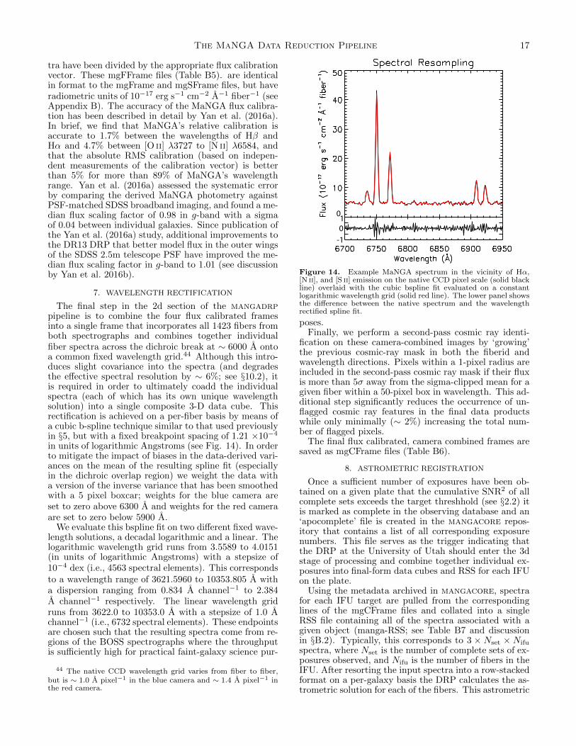
The MaNGA Data Reduction Pipeline 17

tra have been divided by the appropriate flux calibrationvector. These mgFFrame files (Table B5). are identicalin format to the mgFrame and mgSFrame files, but haveradiometric units of 10−17 erg s−1 cm−2 A−1 fiber−1 (seeAppendix B). The accuracy of the MaNGA flux calibra-tion has been described in detail by Yan et al. (2016a).In brief, we find that MaNGA’s relative calibration isaccurate to 1.7% between the wavelengths of Hβ andHα and 4.7% between [O ii] λ3727 to [N ii] λ6584, andthat the absolute RMS calibration (based on indepen-dent measurements of the calibration vector) is betterthan 5% for more than 89% of MaNGA’s wavelengthrange. Yan et al. (2016a) assessed the systematic errorby comparing the derived MaNGA photometry againstPSF-matched SDSS broadband imaging, and found a me-dian flux scaling factor of 0.98 in g-band with a sigmaof 0.04 between individual galaxies. Since publication ofthe Yan et al. (2016a) study, additional improvements tothe DR13 DRP that better model flux in the outer wingsof the SDSS 2.5m telescope PSF have improved the me-dian flux scaling factor in g-band to 1.01 (see discussionby Yan et al. 2016b).

7. WAVELENGTH RECTIFICATION

The final step in the 2d section of the mangadrppipeline is to combine the four flux calibrated framesinto a single frame that incorporates all 1423 fibers fromboth spectrographs and combines together individualfiber spectra across the dichroic break at ∼ 6000 A ontoa common fixed wavelength grid.44 Although this intro-duces slight covariance into the spectra (and degradesthe effective spectral resolution by ∼ 6%; see §10.2), itis required in order to ultimately coadd the individualspectra (each of which has its own unique wavelengthsolution) into a single composite 3-D data cube. Thisrectification is achieved on a per-fiber basis by means ofa cubic b-spline technique similar to that used previouslyin §5, but with a fixed breakpoint spacing of 1.21 ×10−4

in units of logarithmic Angstroms (see Fig. 14). In orderto mitigate the impact of biases in the data-derived vari-ances on the mean of the resulting spline fit (especiallyin the dichroic overlap region) we weight the data witha version of the inverse variance that has been smoothedwith a 5 pixel boxcar; weights for the blue camera areset to zero above 6300 A and weights for the red cameraare set to zero below 5900 A.

We evaluate this bspline fit on two different fixed wave-length solutions, a decadal logarithmic and a linear. Thelogarithmic wavelength grid runs from 3.5589 to 4.0151(in units of logarithmic Angstroms) with a stepsize of10−4 dex (i.e., 4563 spectral elements). This correspondsto a wavelength range of 3621.5960 to 10353.805 A witha dispersion ranging from 0.834 A channel−1 to 2.384A channel−1 respectively. The linear wavelength gridruns from 3622.0 to 10353.0 A with a stepsize of 1.0 Achannel−1 (i.e., 6732 spectral elements). These endpointsare chosen such that the resulting spectra come from re-gions of the BOSS spectrographs where the throughputis sufficiently high for practical faint-galaxy science pur-

44 The native CCD wavelength grid varies from fiber to fiber,but is ∼ 1.0 A pixel−1 in the blue camera and ∼ 1.4 A pixel−1 inthe red camera.

0

0

1

-1

Figure 14. Example MaNGA spectrum in the vicinity of Hα,[N ii], and [S ii] emission on the native CCD pixel scale (solid blackline) overlaid with the cubic bspline fit evaluated on a constantlogarithmic wavelength grid (solid red line). The lower panel showsthe difference between the native spectrum and the wavelengthrectified spline fit.

poses.Finally, we perform a second-pass cosmic ray identi-

fication on these camera-combined images by ‘growing’the previous cosmic-ray mask in both the fiberid andwavelength directions. Pixels within a 1-pixel radius areincluded in the second-pass cosmic ray mask if their fluxis more than 5σ away from the sigma-clipped mean for agiven fiber within a 50-pixel box in wavelength. This ad-ditional step significantly reduces the occurrence of un-flagged cosmic ray features in the final data productswhile only minimally (∼ 2%) increasing the total num-ber of flagged pixels.

The final flux calibrated, camera combined frames aresaved as mgCFrame files (Table B6).

8. ASTROMETRIC REGISTRATION

Once a sufficient number of exposures have been ob-tained on a given plate that the cumulative SNR2 of allcomplete sets exceeds the target threshhold (see §2.2) itis marked as complete in the observing database and an‘apocomplete’ file is created in the mangacore repos-itory that contains a list of all corresponding exposurenumbers. This file serves as the trigger indicating thatthe DRP at the University of Utah should enter the 3dstage of processing and combine together individual ex-posures into final-form data cubes and RSS for each IFUon the plate.

Using the metadata archived in mangacore, spectrafor each IFU target are pulled from the correspondinglines of the mgCFrame files and collated into a singleRSS file containing all of the spectra associated with agiven object (manga-RSS; see Table B7 and discussionin §B.2). Typically, this corresponds to 3 × Nset × Nifu

spectra, where Nset is the number of complete sets of ex-posures observed, and Nifu is the number of fibers in theIFU. After resorting the input spectra into a row-stackedformat on a per-galaxy basis the DRP calculates the as-trometric solution for each of the fibers. This astrometric

18 Law et al.

calibration has two stages: a basic module that computesfiber locations based on reference metadata and theoreti-cal refraction models, and an advanced module that fine-tunes the zero-point location and rotation of the basicsolution by registering the spectra against SDSS broad-band photometry.

8.1. Basic Astrometry Module

The effective location of a particular IFU fiber in anygiven exposure is dictated by numerous optomechanicalfactors. Many of these are possible to either measure orestimate for an arbitrary source, and the MaNGA basicastrometry module combines these factors into a singlewavelength-dependent position vector (in RA/DEC) foreach fiber. These factors include:

1. Relative and absolute fiber location within a givenIFU ferrule based on the as-built fiber bundlemetrology. This is measured during the manufac-turing process to a typical accuracy ∼ 0.3µm (rel-ative)45 and ∼ 5µm (absolute) (see Drory et al.2015) and recorded in mangacore for each har-ness serial number.

2. Offset of an IFU from its base position due to thethree-point dithering pattern. We assume that thedithering exactly matches the commanded offsets;the accuracy of this assumption is limited by the∼ 0.1 arcsec dithering accuracy of the telescope(see Law et al. 2015).

3. Offset of drilled holes from the intended drillinglocation. Although holes can be drilled to withinan accuracy of ∼ 9µm rms, they are measured afterthe fact to an accuracy ∼ 5µm. This informationis recorded for each plate in mangacore.

4. Chromatic differential atmospheric refraction(DAR) relative to the guide wavelength (∼ 5500A). This shifts the effective location of each fiberas a function of wavelength (i.e., a given fiberreceives light from a different part of a targetgalaxy at blue versus red wavelengths). Themagnitude and direction of this effect is calculatedusing the SDSS plate design code model (basedin part on Filippenko 1982) as discussed in detailby Law et al. (2015) and depends on the alti-tude, the parallactic angle, and the atmospherictemperature/pressure/humidity. We calculate theexpected effect at the midpoint of a given exposurefor each of the 4563 wavelength channels (for thelogarithmic case) given the known location ofeach IFU on the sky and atmospheric conditionsrecorded in the headers of individual exposures.

5. Global shift of the IFU location at the guide wave-length due to field differential atmospheric refrac-tion. Over the 3 field of an SDSS plate there arechanges in scale and rotation of the sky image (inparticular, altitude-dependent compression alongthe altitude axis). The telescope guiding softwarecorrects for these effects averaged over the plate,

45 0.3µm corresponds to 5 milliarcsec at the SDSS focal plane(∼ 60µm arcsec−1)

but cannot fully correct the quadrupole distortionin the effective location of a given IFU. We esti-mate this effect as discussed in detail by Law et al.(2015).

6. Wavelength-dependent distortions due to the SDSStelescope optics. These are estimated based onupon optical models of the telescope in the SDSSplate design code (Gunn et al. 2006).

The final product of the basic astrometry module is apair of two-dimensional arrays (matched in size to themgCFrame flux array) that give the X and Y fiber posi-tions (in units of arcsec in the tangent plane) relative tothe nominal IFU center IFURA, IFUDEC. These arrayscan thereafter be used to look up the effective on-skylocation corresponding to any wavelength, for any fiber.

8.2. Extended Astrometry Module

During operations within a single dark run a MaNGAcartridge will remain plugged with a given plate untilobservations for that plate are complete. Since MaNGAshares carts with APOGEE-2N however, at the end of adark run it is typically necessary to unplug the MaNGAIFUs from unfinished plates and replug them again thefollowing dark run to continue observations. This replug-ging introduces an uncertainty into the relative center-ing and rotation of each IFU in its hole at the level of∼ 0.5 arcsec (centering) and ∼ 2 − 3 (rotation) fromthe required clearance of locator pins within their holes.The precise change cannot be measured directly and willchange from plugging to plugging as it depends on thetorsional stresses arising from the routing of each IFUcable through a cartridge. Such uncertainties46 are sig-nificantly larger than any of the uncertainties derivedfrom effects described in §8.1.

We therefore follow the method employed by theVENGA survey (Blanc et al. 2013) of registering thefiber spectra from each exposure against SDSS broad-band imaging. In this ‘extended astrometry module’(EAM) we compute the synthetic broad-band flux of eachfiber by integrating the flux-calibrated spectrum over thecorresponding transmission curve. We then search a gridin right ascension, declination, and rotation of the fiberbundle relative to the base position determined in §8.1(we keep the relative positions of fibers within the bun-dle fixed). At each position on the grid the fiber co-ordinates (collapsed from the basic astrometry solutionover the appropriate wavelength range) are shifted ac-cordingly, and aperture photometry is performed on aPSF matched SDSS broadband image using 2.0 arcsecdiameter apertures for each fiber. An additional overallflux normalization is permitted according to

fSDSS = AfMaNGA +B (1)

where fSDSS and fMaNGA are the SDSS broadband andMaNGA fiber fluxes respectively, A is a multiplicativescaling factor, and B represent a zeropoint shift.47 Yan

46 At the outer ring of a 127-fiber IFU such a 3 degree rotationaluncertainty corresponds to ∼ 0.8 arcsec.

47 We note that these A and B terms are derived for informa-tional purposes only; we do not apply corrections from them tothe data but rather use them as an independent check on the flux

The MaNGA Data Reduction Pipeline 19

et al. (2016a) presented a discussion of these A and Bcoefficients, and determined that A had a roughly gaus-sian distribution centered about 1.00 (in i-band) with asigma of 0.037 for ∼ 25, 000 IFU-exposures obtained dur-ing the first year of operations, indicating that the spec-trophotometric accuracy of the MaNGA data is about 4%with respect to the SDSS imaging data. The best-fit val-ues of position, rotation, and flux offsets are determinedvia χ2 minimization, with corresponding uncertaintiesdrawn from the χ2 probability maps. This exercise isrepeated in each of the four g, r, i, and z bands, withthe final result a biweight mean of the four bands (thisprovides robustness against occasional unmasked cosmicrays).

Unsurprisingly, the EAM can achieve better results forlarger fiber bundles on galaxies with significant azimuthalstructure than for smaller bundles on smooth and cir-cular galaxies. In Figure 15 we show EAM results fortwo commissioning galaxies 7443-12703 and 7443-3702.For the large IFU on a source with significant structure(7443-12703) the measurement uncertainties on both po-sitional shift and global rotation are small, and reveal (inthis case) a ∼ 0.5 arcsec shift in the IFU center across acartridge replugging. In contrast, for the small IFU on arotationally symmetric source (7443-3702) the positionalshift is still well constrained but the global rotation isalmost completely unconstrained in the range of valuesexplored by the EAM (±5).

In order to avoid introducing errors into our astrom-etry due to such noisy measurements, we therefore runthe EAM iteratively. In the first pass, each exposure isfitted independently. The derived values of ∆θ are thenaveraged across all exposures in a given plugging, andthe EAM run again holding ∆θ fixed at these averagevalues in order to better determine positional shifts be-tween exposures. Since rotation is expected to changeonly between repluggings (consistent with observed be-havior based on galaxies with sufficient azimuthal struc-ture to measure ∆θ reliably) this allows us to mitigatethe uncertainty in any individual measurement of bundlerotation. In contrast, such averaging is not justified forthe positional shifts. Although such shifts are dominatedby repluggings (e.g., Fig. 15), smaller shifts at the ∼ 0.1arcsec level are possible due to uncertainties in the ap-plied dither offsets that we wish to correct through theEAM. On average, we find that the median astrometricuncertainty of the exposures making up the 1390 galaxiesin DR13 relative to the SDSS preimaging data is ∼ 0.1arcsec (1σ) based on the reduced χ2 surface.

Since each set of three exposures is known to have uni-form coverage (see Law et al. 2015; Yan et al. 2016b)sets from different pluggings of a given plate (and in-deed, even between different cartridges) can therefore becombined together onto a common astrometric solutionusing the EAM. Since all MaNGA target galaxies aredrawn from the SDSS imaging footprint, this correctionis automatically applied to all MaNGA galaxies.48

9. DATA CUBE CONSTRUCTION

calibration of each frame and flag exposures as problematic whereA or B deviate substantially from 1.0 and 0.0 respectively.

48 The method will fail on point-like sources and some ancillarytargets outside the SDSS imaging footprint; for these objects theEAM is disabled and the basic astrometry module is used alone.

9.1. Basic Cube Building

Using the RSS files and associated astrometric solu-tions derived in §8 we combine the individual fiber spec-tra into rectilinearly gridded cubes (with orientation RA,DEC, λ) for each IFU on both logarithmic and linearly-sampled wavelength solutions. Since these input spectrahave already been resampled onto a common wavelengthgrid, this simplifies to the 2-dimensional reconstructionof a regularly-gridded image from an irregularly sampledcloud of measurements of the intensity profile at a givenwavelength channel.

Multiple methods exist for performing such image re-construction (see §9.2); we choose to build our data cubesone image slice at a time using a flux-conserving vari-ant of Shepard’s method similar to that used by theCALIFA pipeline (Sanchez et al. 2012). At each of the4563 wavelength channels (for the logarithmically sam-pled data; 6732 for the linear), we describe our input dataas one-dimensional vectors of intensity f [i] and varianceg[i] with length N = Nfiber × Nexp where Nfiber is thenumber of fibers in the IFU (e.g., 127) and Nexp is thetotal number of exposures to combine together. Simi-larly, we can construct vectors x and y which describethe effective position of the center of each fiber based onthe astrometric solution derived in §8, and converting tofractional pixel coordinates relative to some chosen ori-gin and pixel scale. We adopt a spatial pixel scale of 0.5arcsec pixel−1 and an output grid of size Xmax by Ymax

taken to be slightly larger than the dithered footprint ofthe MaNGA IFU.

Each of the M = Xmax×Ymax pixels in the output im-age can likewise be resorted into a one-dimensional arrayof values, with the pixel locations given by X[j] and Y [j]respectively for j = 1 to M . The mapping between thef [i] intensity measurements in the irregularly-sampledinput and the F [j] intensities in the regularly-sampledoutput image are then determined by the weights w[i, j]describing the relative contribution of each input pointto each output pixel. We take this weight function to bea circular Gaussian:

w[i, j] = b[i] exp

(−0.5

r[i, j]2

σ2

)(2)

where σ = 0.7 arcsec is an exponential scalelength,r[i, j] =

√(x[i]−X[j])2 + (y[i]− Y [j])2 is the distance

between the i’th fiber location and the j’th output gridsquare, and b[i] is a binary integer equal to zero wherethe inverse variance g[i]−1 = 0 and one elsewhere. Es-sentially, b[i] functions as a mask that allows us to ex-clude known bad values in individual spectra from thefinal combined image. Additionally, we set w[i, j] = 0for all r[i, j] > rlim = 1.6 arcsec as an upper limit on theradius of influence of any given measurement. These lim-iting radii and scale lengths are chosen empirically basedon observed performance; the present values are foundto provide the smallest reconstructed FWHM for stel-lar targets observed as part of commissioning (see §10.1)whilst not introducing spurious structures by shrinkingthe impact-radius of individual fibers too severely.

In order to conserve flux we must normalize the weightssuch that the sum of the weights contributing to anygiven output pixel is unity. The normalized weight func-

20 Law et al.

Exposure Number

Δα

(a

rcse

c)

Δδ

(a

rcse

c)

Δθ

(d

eg

ree

s)

Exposure Number Exposure Number

Exposure Number Exposure Number Exposure Number

Δα

(a

rcse

c)

Δδ

(a

rcse

c)

Δθ

(d

eg

ree

s)

WE

N

S

5’’

7443−12703

WE

N

S

5’’

7443−3702

Figure 15. MaNGA EAM performance for two commissioning galaxies 7443-12703 and 7443-3702 (mangaid 12-193481 and 12-84670respectively). The left-most panel shows a 3 color image of each galaxy based on SDSS imaging data, overlaid with a hexagonal boundingbox indicating the footprint of the MaNGA IFU. The remaining boxes show the values calculated by the EAM for the relative shift inright ascension, declination, and bundle rotation between exposures (open black boxes with associated 1σ uncertainties). Red boxes in theright-hand panel show the average values in ∆θ adopted for all exposures in a given plugging in a second run of the EAM. Values shownfor the shifts ∆α and ∆δ are after this second-pass with fixed ∆θ. The vertical dotted line represents a replugging of the plate betweenexposures 9 and 10.

tion is therefore:

W [i, j] =w[i, j]∑Ni=1 w[i, j]

(3)

where in order to avoid divide by zero errors we setW [i, j] = 0 where w[i, j] = 0 for all i in the range 1to N (e.g., outside the hexagonal footprint of the IFU).

The intensity distribution of the pixels in the outputimage may therefore be written as the matrix product ofthe normalized weights and the input intensity vector:

F = αW × f = α

W11 . . . WN1...

. . ....

W1M . . . WNM

× f1

...fN

(4)

or alternatively as

F [j] = α

N∑i=1

f [i]W [i, j] (5)

where α = 1/(4π) is a constant factor to account for theconversion from flux per unit fiber area (π arcsec2) toflux per unit spaxel area (0.25 arcsec2). The resultingF [j] may then trivially be rearranged to form the outputimage at this wavelength slice given the known mappingof the pixel coordinates X[j] and Y [j].

Similarly, the variance G of the rectified output imagemay be written as

G[j] = α2N∑i=1

g[i] (W [i, j])2 (6)

This calculation therefore propagates the uncertaintiesin individual spectra through to the final data cube, but

does not use these uncertainties in constructing the com-bined flux values (except for the simple masking of badvalues where inverse variance is equal to zero).

These rectified images of the intensity profile andthe corresponding inverse variance maps at each wave-length channel are reassembled by the DRP into three-dimensional cubes along with a 3d quality mask describ-ing the effective coverage and data quality of each spaxel.The final manga-CUBE files are discussed further in §B.2(see also Table B8).

9.2. Algorithm Choice

As stated in §9.1, there are multiple algorithms that wecould have adopted for building our data cubes, rangingfrom surface fitting techniques (e.g., thin plate spline fits)to drizzling and our adopted modified Shepard approach.Based on idealized numerical simulations performed priorto the start of the survey we found that the surface-fittingapproach provided reasonable quality reconstructed im-ages, but was nonetheless undesirable because there isno simple means by which to propagate uncertainties inthe resulting surface. In contrast, the modified Shepardapproach allows for easy calculation of both the varianceand covariance of the reconstructed data cubes, as de-scribed in §9.3.

The drizzle approach (Fruchter & Hook 2002) has beentested by ourselves and by the CALIFA (Sanchez et al.2012) and SAMI (Sharp et al. 2015) surveys, all of whomhave found that (1) it broadened the final PSF, and (2)since fiber bundle IFUs have < 100% fill factor in a givenexposure it can create artificial structures in the intensitydistribution following the footprint of the circular fibers.To mitigate this problem the SAMI survey (see discus-sion by Sharp et al. 2015) adopted a weighting systembased on the ratio between the original fiber area andthe area covered by a final spaxel of a particular fiber (if

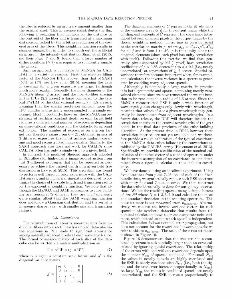
The MaNGA Data Reduction Pipeline 21

the fiber is reduced by an arbitrary amount smaller thanthe original size). This in essence redistributes the fluxfollowing a weighting that depends on the distance tothe centroid of the fiber and is truncated at a maximumdistance controlled by the arbitrary reduction of the cov-ered area of the fibers. This weighting function results insharper images, but in order to smooth out the artificialstructure in the intensity distribution Sharp et al. (2015,see their Figs. 7 and 9) found that a large number ofdither positions (≥ 7) was required to sufficiently samplethe galaxy.

Such an approach is not viable for MaNGA (or CAL-IFA) for a variety of reasons. First, the effective fillingfactor of the MaNGA IFUs is lower than that of SAMI(56% vs 75%; see Law et al. 2015), meaning the gapsin coverage for a given exposure are larger (althoughmuch more regular). Secondly, the inner diameter of theMaNGA fibers (2 arcsec) and the fiber-to-fiber spacingin the IFUs (2.5 arcsec) is large compared to the typ-ical FWHM of the observational seeing (∼ 1.5 arcsec),meaning that the spatial resolution incident upon theIFU bundles is drastically undersampled in a single ex-posure. Most importantly, however, the MaNGA surveystrategy of reaching constant depth on each target fieldrequires a different total number of exposures dependingon observational conditions and the Galactic foregroundextinction. The number of exposures on a given tar-get can therefore range from 6 – 21, obtained in sets of3 dithered exposures that must achieve uniform cover-age and good reconstructed image quality. Similarly, theSAMI approach also does not work for CALIFA sinceCALIFA often has only a single visit to a given field.

In contrast, the modified Shepard approach adoptedin §9.1 allows for high-quality image reconstruction fromjust 3 dithered exposures that can be repeated as nec-essary to achieve the desired depth in a given field (seediscussion in Law et al. 2015). This algorithm was foundto perform well based on prior experience with the CAL-IFA survey, and in numerical simulations designed to op-timize the choice of the scale length and truncation radiusfor the exponential weighting function. We note that al-though the MaNGA and SAMI approaches to cube build-ing are conceptually different they are mathematicallyquite similar, albeit that the SAMI weighting functiondoes not follow a Gaussian distribution and the kernel isin essence sharper (i.e., with smaller size and truncationradius).

9.3. Covariance

The redistribution of intensity measurements from in-dividual fibers into a rectilinearly-sampled datacube viathe equations in §9.1 leads to significant covarianceamong spatially adjacent pixels at each wavelength slice.The formal covariance matrix of each slice of the datacube can be written via matrix multiplication as:

C = α2W × (g′ ×W ᵀ) (7)

where α is again a constant scale factor, and g′ is thediagonal variance matrix

g′ =

g1 0 . . . 00 g2 . . . 0...

.... . .

...0 0 . . . gN

(8)

The diagonal elements of C represent the M elementsof the variance array G[j] for the output image while theoff-diagonal elements of C represent the covariance intro-duced between different pixels in the output image by thechosen weighting method. These may in turn be recastas the correlation matrix ρ, where ρjk = Cjk/

√CjjCkk

for all j and k from 1 to M . ρ is thus unity along thediagonal elements (since each pixel has unity correlationwith itself). Following this exercise, we find that, gen-erally, pixels separated by 0.′′5 (1 pixel) have correlationcoefficients of ρ ≈ 0.85, decreasing to ρ < 0.1 (i.e., nearlyuncorrelated) at separations of ≥ 2 arcsec. Spatial co-variance therefore becomes important when, for example,one calculates the inverse variance in a spectrum gener-ated by coadding many adjacent spaxels.

Although ρ is nominally a large matrix, in practiceit is both symmetric and sparse, containing mostly zero-valued elements since we have truncated the weight func-tion to be zero outside a radius of 1.6 arcsec. Since theMaNGA reconstructed PSF is only a weak function ofwavelength ρ also changes only slowly with wavelength,meaning that values of ρ at a given wavelength may gen-erally be interpolated from adjacent wavelengths. In afuture data release, the DRP will therefore include thecorrelation matrix at the central wavelengths of the grizbands in the final data products of the cube buildingalgorithm. At the present time in DR13 however thesecorrelation matrices are not yet available, and we there-fore provide a rough calibration of the typical covariancein the MaNGA data cubes following the conventions es-tablished by the CALIFA survey (Husemann et al. 2013).Specifically, we provide a calibration of the nominal cal-culation of the noise vector of a coadded spectrum underthe incorrect assumption of no covariance to one deter-mined from a rigorous calculation that includes covari-ance.

We have done so using an idealized experiment. Usingfive datacubes from plate 7495, one of each of the fiber-bundle sizes, we synthetically replace each RSS spectrumwith unity flux and Gaussian error. We then constructthe datacube identically as done for our galaxy observa-tions. We bin the resulting spaxels using a simple boxcarof size N2 where N = 1, 3, 5, 7, 9 and calculate the meanand standard deviation in the resulting spectrum. Thisnoise estimate is our measured error, nmeasured. Alterna-tively, we can use the inverse-variance vectors for eachspaxel in the synthetic datacube that results from thenominal calculation above to create a separate noise esti-mate, which instead assumes each spaxel is independent.This calculation follows nominal error propagation, butdoes not account for the covariance between spaxels; werefer to this as nno covar. The ratio of these two estimatesis shown in Figure 16.

Figure 16 demonstrates that the true error in a com-bined spectrum is substantially larger than an error cal-culated by ignoring spatial covariance. The relationshipof the errors with and without covariance depends uponthe number Nbin of spaxels combined. For small Nbin

the values in nearby spaxels are highly correlated andthe SNR is nearly constant with Nbin (i.e., both the sig-nal and the true error increase proportionally to Nbin).At large Nbin the values in combined spaxels are nearlyuncorrelated, and the SNR increases proportionally to

22 Law et al.

√Nbin.We have thus fit a functional form identical to that

used by Husemann et al. (2013) to our measurements inFigure 16 and find that

nmeasured/nno covar ≈ 1 + 1.62 log(Nbin), (9)

for Nbin . 100, and

nmeasured/nno covar ≈ 4.2 (10)

for Nbin > 100 (i.e., beyond ∼ 2 times the FWHM wherespaxels are uncorrelated).

It is important to note that the binned spaxels mustbe adjacent for this calibration to hold; i.e., a randomselection of spaxels across the face of the IFU will notshow as significant an effect because they will not be asstrongly covariant. The inset histogram shows the ratioof the data to the fitted model in equation 9, demon-strating the calibration is good to about 30%. We haveconfirmed this result empirically by comparing the stan-dard deviation of the residuals of the best-fitting contin-uum model for a large set of galaxy spectra, followingan approach similar to Husemann et al. (2013). How-ever, we emphasize that the test we have performed toproduce Figure 16 is more idealized and controlled. Wealso confirm that a rigorous calculation of the covariance,following the matrix multiplication discussed at the be-ginning of this section, and a subsequent calculation ofthe noise vector in the binned spectra used in Figure 16are fully consistent with our meausurements nmeasured.

10. DATA QUALITY

10.1. Data Cubes: Angular Resolution

An estimate of the spatial light profile of an unresolvedpoint source (i.e., the ‘reconstructed PSF’) is automati-cally provided for each data cube using a numerical sim-ulation tied to the specific observing conditions of eachexposure. Using the known fiber locations for a givenexposure, the DRP computes the flux expected to berecorded by each fiber from an unresolved point sourcelocated at the center of the IFU. This model flux is basedon integration of the nominal PSF incident on the face ofthe IFU in the focal plane of the SDSS 2.5m telescope.The focal-plane PSF is taken to be a double-gaussianthat accounts for chromatic distortions due to the tele-scope optics and observational seeing recorded by theguide camera. As detailed by Yan et al. (2016a), sincethe guide-camera reports image FWHM systematicallylarger than measured by the MaNGA IFU fiber bundles,the guider seeing measurements are also ‘shrunk’ by ascale factor determined by the flux calibration module togive an incident PSF that best matches differential fiberfluxes recorded by the 12 photometric standard star mini-bundles. These simulated fiber fluxes are reconstructedinto a data cube using the same algorithm as the sciencedata, and slices of this cube corresponding to g, r, i, zbands are attached to each data cube.

These griz images (GPSF, RPSF, IPSF, ZPSF; see§B.2) provide a reasonable estimate of the reconstructedPSF in each data cube and are reported in each of theFITS headers. We confirmed the fidelity of these re-constructed PSF models by observing a plate duringsurvey commissioning in which every MaNGA IFU tar-geted bright stars with two sets of dithered observations

Figure 16. Ratio of the measured noise in a synthetic datacube,nmeasured, (see text) to a nominal calculation of the noise in abinned spectrum that does not include covariance, nno covar, as afunction of the number of spaxels included in the combined spec-trum, Nbin. The point color provides the size of the boxcar used tocreate the bin. Nominally, Nbin = N2, however some boxcar win-dows fell outside of the IFU field-of-view in the synthetic datacube.The equation at the bottom right gives the best-fitting calibrationof nno covar to nmeasured for values of Nbin ≤ 100. The inset his-togram shows the ratio of the model to the data, demonstratingthe calibration is good to about 30%.

(i.e., following the methodology of typical galaxy obser-vations). This plate (7444) was processed by the DRPin an identical manner to standard galaxy plates, withthe exception that only the basic astrometry module wasused to register the fiber locations since there is no ex-tended structure against which to use extended astrom-etry module.

In Figure 17 we show the profiles of stars in four ofthe reconstructed data cubes compared to the simulatedestimates. We find that the actual reconstructed PSF ofthese data cubes is well described by a single 2d gaussianfunction with normalized intensity

I(r) =1

2πσ2exp

(−r2/2σ2

)(11)

where 2.35σ is the standard gaussian FWHM. This pro-file is well matched to the model PSF estimated basedon mock integrations of an artificial point source at theknown fiber positions; the model FWHM estimates agreewith the measured values to within 1-2%. The measuredFWHM of the reconstructed PSF for the other 13 IFUson plate 7444 similarly lie in the range 2.4−2.5 arcsec.49

Based on the simulations presented by Law et al. (2015)

49 Except for one 19-fiber IFU, for which the reconstructed imageis clearly out of focus, indicating that it partially fell out of the

The MaNGA Data Reduction Pipeline 23

and the range of Ω uniformity values for DR13 reportedby Yan et al. (2016b) we expect that the reconstructedPSF FWHM should vary by less than 10% across a givenIFU.

As discussed in greater detail by Yan et al. (2016b),the range of g-band reconstructed PSF FWHM in the1390 DR13 galaxy data cubes is generally distributed inthe range 2.2 − 2.7 arcsec, with a tail to about 3 arcsec(Figure 17).

10.2. Data Cubes: Spectral Resolution

As indicated in §4.2.5, the line spread function variesalong the spectrograph slit, and hence varies spatiallywithin a given IFU. Similarly, the LSF can also varybetween exposures with ambient temperature drifts andchanges in the focus of the spectrograph. The typicalspectral resolution for DR13 galaxies is shown in Figure18; typical IFUs show rms variability at the level of 1−2%(blue shaded region), while the worst-case large IFUs onthe ends of the spectrograph slit can show variability ashigh as 8−10% at blue wavelengths (red shaded region).This variability within the worst-case IFUs is dominatedby the along-slit variability, but compounded by varia-tions between exposures. The focus in the red camerasis significantly flatter than in the blue cameras, meaningthat variation in spectral resolution longward of 6000 Ais 1% or less even for the worst-case IFUs.50

Each MaNGA data cube therefore has an associatedextension (see §B.2) describing both the mean and 1σdeviation about the mean spectral resolution for all fiberspectra contributing to the cube. Detailed informationon spectral resolution of the individual fiber spectra usedto create a given data cube are contained in the final RSSfiles.

After finalization of the DR13 data pipeline it was re-alized that the instrumental LSF estimates reported bythe pipeline are systematically underestimated. Thereare two factors that contribute to this underestimation;first, the LSFs reported in DR13 correspond to nativegaussian widths prior to convolution with the boxcar de-tector pixel boundaries (i.e., the gaussian function is in-tegrated over the pixel boundaries), while many third-party analysis routines simply evaluate gaussian modelsat the pixel midpoints. Although neither approach isnecessarily more ‘correct’ than the other, this nonethe-less represents a systematic difference between the val-ues quoted and the values that would be measured withmost third-party routines. Second, the wavelength recti-fication performed in §7 effectively resamples the spectraand introduces a broadening into the LOG and LINEARformat spectra that is not accounted for by the DR13data pipeline. These issues are not unique to the MaNGAdata and pipeline, but rather affect all previous genera-tions of SDSS optical fiber spectra as well.

Efforts to address this discrepancy are ongoing (see,e.g., Westfall et al. in prep) and will be detailed in a fu-ture version of the MaNGA data pipeline. In the presentcontribution, we note that re-analysis of ∼ 2500 individ-ual exposures suggests that multiplying the DR13 LSF

plate. Such cases are rare, and detected during quality-controlchecks by the extended astrometry module.

50 Except around 8100 A where the red detectors have a two-phase discontinuity (see §4.2.5).

by a factor of 1.10 gives a reasonable first-order correc-tion (i.e., the spectral resolution of the DR13 data prod-ucts is overestimated by ∼ 10%). This correction factoraccounts for both the pre- vs post-pixellization gaussiandifference (∼ 4%) and the wavelength rectification broad-ening (∼ 6%).

10.3. Wavelength calibration

Based on previous calculations for the BOSS redshiftsurvey (e.g., Bolton et al. 2012, their Figure 14), theMaNGA spectra (which share the same instrument andmuch of the same reduction pipeline software) shouldalso have absolute wavelength calibration good to ∼ 5km s−1. We verify this estimate by comparing brightemission line features in the MaNGA data cubes againstpublicly-available SDSS-I single fiber spectra of each ofthe galaxies in DR13. For each galaxy, we obtain thecorresponding SDSS-I spectrum from SkyServer51 , anddetermine the effective location of the spectrum from thePLUG RA and PLUG DEC header keywords. We thenperform aperture photometry in a 2 arcsec circular ra-dius about this location at every wavelength slice of theMaNGA data cube in order to construct a 1d MaNGAspectrum of the central pointing. Both the SDSS-I andMaNGA spectra are then fitted with single-Gaussianemission line components at the expected wavelengthsof the Hβ, [O iii] λ5007, Hα, and [N ii] λ6583 nebularemission lines given the known galaxy redshift from theNASA-Sloan Atlas (NSA; Blanton et al. 2011).52

Although many of the MaNGA galaxies do not havestrong emission line features in their central spectra, suf-ficiently many do in order to allow us to statisticallycompare the MaNGA and SDSS-I spectra. Consideringonly galaxies for which both MaNGA and SDSS fits arewithin 5 A of the nominal wavelength, have σ width of0.5 to 5 A, and line fluxes > 10−16 erg s−1 cm−2, wefind that 470/670/760/1063 galaxies fulfill the criteriafor Hβ,[O iii],Hα, and [N ii] respectively. In Figure 19 weplot the distribution of relative peak velocity offsets foreach of these 4 emission lines. We conclude that thereis no systematic offset between the MaNGA and SDSS-Ispectra to within ∼ 2 km s−1, and that individual galax-ies are distributed nearly according to a Gaussian with1σ width ∼ 10 km s−1.

This width may in part however reflect intrinsic ve-locity gradients within the galaxies combined with un-certainties at the few tenths of an arcsecond level in theeffective location of the SDSS-I fibers due to hardwaretolerances and differential atmospheric refraction.53 Us-ing the MaNGA IFU spectra, we find that changes inlocation at the level of just 0.25 arcsec (compared to thetypical MaNGA astrometric uncertainty of 0.1 arcsec;see §8.2) can easily result in ∼ 20 km s−1 velocity shiftsin the resulting spectra for galaxies with strong centralvelocity gradients (e.g., 8453-12703). The actual wave-length accuracy of the MaNGA spectra may thereforemore accurately be given by the rms agreement between

51 SkyServer is a web-based public interface to the SDSS archive;see http://skyserver.sdss.org/dr12/en/home.aspx

52 http://www.nsatlas.org53 Indeed, the SDSS-I spectra also have effective locations that

change as a function of wavelenth due to chromatic atmosphericrefraction.

24 Law et al.

7444-12701

Δ R.A. (arcsec)

Δ D

ec

l. (

arc

sec

)

+15 -150

0

+15

-15

Figure 17. Top right panel: Reconstructed image of a bright star observed in standard dithered observations (7444-12701); the data cubehas been collapsed over wavelength channels 300-700 (λλ3881− 4255 A). The greyscale stretch is logarithmic to illustrate the symmetricalnature of the extended profile wings. Left-hand panels: radial profiles of bright stars targeted by four of the largest IFUs on plate 7444. Blackpoints show the radial profile of the reconstructed image (based on collapsing the corresponding data cube over the range λλ3881 − 4255A). The solid red lines show the best 2d gaussian fitted to the black points, with characteristic FWHM and minor/major axis ratio (b/a)indicated. The dashed red lines show the corresponding 2d gaussian fitted to the PSF model provided by the pipeline based on known fiberlocations and observing conditions for each exposure. Lower right panel: Distribution of g-band FWHM measured for all 1390 galaxy datacubes in DR13; vertical dashed line indicates the median of 2.54 arcsec.

repeat MaNGA observations of a small sample of galaxiesin DR13; indeed, although there are only ∼ 10 repeat-observations with strong emission lines in DR13 we finda typical rms agreement of 5 km s−1 between the fouremission line wavelengths above.

The relative wavelength calibration accuracy of the in-dividual fibers within a given IFU is more difficult to as-sess in the absence of a calibration reference. However,we can obtain a rough estimate by considering the rmsscatter between the measured centroids of bright skylinesand the fitted value adopted by the pipeline as describedin §4.3. As a conservative estimate,54 we assume thatthe smallest rms amongst the individual skyline mea-surements is indicative of the relative wavelength calibra-tion accuracy. At 0.024 pixels at 8885 A, this suggests arelative fiber-to-fiber wavelength calibration accuracy ofbetter than 1.2 km s−1 rms.

54 The rms of any individual line is closely related to the strengthof the line (stronger lines have smaller rms), and the wavelengthsolution is based upon a fit to many such lines (both skylines andarc lamp lines).

10.4. Typical depth

Finally, we illustrate the overall quality of the MaNGAspectral data by comparing the spectrum of the centralregion of galaxy 7443-12704 (aka UGC 09873) from theMaNGA commissioning plate against previous SDSS-Isingle-fiber and CALIFA55 DR-2 (Garcıa-Benito et al.2015; Walcher et al. 2014; Sanchez et al. 2012) IFU ob-servations of the same galaxy. Such a direct compari-son is intrinsically difficult as the total flux in a givencircular aperture is strongly affected by both the obser-vational seeing and chromatic differential refraction (forSDSS-I) and by the effective spatial resolution of the re-construction data cubes (MaNGA and CALIFA), espe-cially in regions of the galaxy where there is a stronggradient in the intrinsic surface brightness (i.e., near thecenter). This method is therefore good for comparing the

55 Based on observations collected at the Centro AstronomicoHispano Aleman (CAHA) at Calar Alto, operated jointly bythe Max-Planck-Institut fur Astronomie and the Instituto de As-trofısica de Andaluca (CSIC). See http://califa.caha.es/

The MaNGA Data Reduction Pipeline 25

Figure 18. MaNGA spectral resolution (FWHM) as a function of wavelength for the final wavelength-rectified data products. The solidblack line represents the average FWHM across all 1390 galaxy data cubes in DR13, while the grey shaded region indicates the minimumand maximum FWHM of all 11,916 fiber spectra obtained for example plate 8588. Blue dark/light shaded regions and red dark/lightshaded regions show the 1σ/2σ variations about the the least-variable and most-variable IFUs on this plate respectively (8588-12704 and8588-12705). The dotted/dashed black lines indicate the final pixel sampling scale of the MaNGA LOG-format and LINEAR-format datarespectively. The solid grey lines represent the native pixel sampling of the blue and red cameras. The feature around 8100 A indicatesthe two-phase detector discontinuity. Note that the values shown here have been broadened by 10% relative to the values reported by theDR13 data pipeline to account for post-pixellization modeling and wavelength rectification (see discussion in §10.2).

HαHβ

[N II][O III]

2 ± 9

km/s

0 ± 13

km/s

-2 ± 9

km/s

-2 ± 8

km/s

Figure 19. Histograms of velocity difference between SDSS-Ispectra and MaNGA IFU spectra extracted from a 2 arcsec radiuscircular aperture centered on the location of the SDSS-I spectra.The 4 panels show the results for Hβ, [O iii] λ5007, Hα, and [N ii]λ6583 for the 1351 unique galaxies in DR13. Note that the manygalaxies with nebular emission lines too weak for reliable measure-ment have been omitted from the distribution. Black histogramsin each panel show the observed distribution, while red histogramsillustrate the best-fit Gaussian model. The values in each panelgive the center and 1σ width of the Gaussian model; this widthmay be driven largely by internal velocity gradients paired withuncertainties in the SDSS-I fiber locations.

relative shapes of spectra from different surveys, but notthe overall normalization of the flux calibration (whichshould instead be assessed through PSF-matched broad-band imaging, e.g., Yan et al. 2016a).

In this case, the SDSS-I spectrum (observed in May2004, and obtained from the DR-12 Science ArchiveServer) corresponds to a circular fiber with core diameter3 arcsec observed in ∼ 1.6 arcsec seeing. In contrast, theMaNGA and CALIFA cubes have an effective FWHM of∼ 2.5 arcsec, meaning that for a centrally concentrated

source there will be systematically less flux within a 3arcsec diameter aperture within these cubes than in theoriginal SDSS-I single-fiber spectrum. We therefore ex-tract the corresponding MaNGA and CALIFA spectra ina 5-arcsec diameter circular aperture about the nominallocation of the SDSS-I spectrum, and additionally allowfor a constant multiplicative scaling factor between all ofthe spectra (derived from the average ratio of the spectrainterpolated to a common wavelength solution).

In Figure 20 we plot the resulting spectra for the SDSS-I (red line), SDSS-IV/MaNGA (black line), and CALIFAR ∼ 850 (green line) and R ∼ 1650 (blue line) data.Although we cannot assess the absolute flux calibrationfrom this plot, we note that the relative flux calibrationbetween the four spectra is in extremely good agree-ment. In the regions of common wavelength coverage,all four spectra show similar structure in the continuumand the emission/absorption lines, with the exception ofa known downturn due to vignetting in the CALIFA low-resolution spectrum longwards of 7100 A. Figure 20 alsoclearly demonstrates the longer wavelength baseline andhigher SNR (especially in the far blue) of the MaNGAdata compared to both SDSS-I and CALIFA.

Additionally, we estimate the typical sensitivity of theMaNGA data cubes based on the inverse variance re-ported by the pipeline for regions far along the minoraxis away from edge-on disk galaxy 8465-12704. We esti-mate the typical continuum surface brightness sensitivityby taking the square root of the sum of the variances ofcube spaxels within 5 arcsec diameter region, multiply-ing by a covariance correction factor based on the numberof spatial elements summer (see Eqn. 9), and convert-ing the resulting 1σ flux sensitivity to a 10σ sensitivityin terms of AB surface brightness. Similarly, to deter-mine the typical 5σ point source emission line sensitivitywe sum the variance over twice the FWHM of the line

26 Law et al.

WE

N

S

5’’

Figure 20. Central spectrum of galaxy 7443-12704 (UGC 09873) extracted from the SDSS-IV MaNGA IFU data cube (black line)compared to the co-located SDSS-I single fiber spectrum (red line). For comparison we also include spectra extracted from the CALIFAhigh-resolution (v1200; blue line) and low-resolution (v500; green line) IFU data cubes. SDSS-I and CALIFA spectra have been offsetvertically from the MaNGA spectrum to aid visual inspection. The inset at lower right shows the SDSS 3-color image of UGC 09873 alongwith an indication of the MaNGA IFU footprint (pink hexagon) and circular spectral extraction region (red circle).

spread function, sum over a 5 arcsec diameter aperture,and multiply the square root of this by a covariance cor-rection factor. We note that both sensitivity estimatesinclude only noise from the detector and background sky,and do not account for any additional noise that may beintroduced by astrophysical sources. As illustrated inFigure 21, the derived sensitivities within a 5 arcsec di-ameter aperture are strong functions of wavelength, vary-ing from about 23.5 AB arcsec−2 and 5× 10−17 erg s−1

cm−2 at blue wavelengths to about 20 AB arcsec−2 and2 × 10−16 erg s−1 cm−2 in the vicinity of the strongestOH skylines.

11. SUMMARY

The 13th data release of the Sloan Digital Sky Surveyincludes the raw MaNGA spectroscopic data, the fullyreduced spectrophotometrically calibrated data, and thepipeline software and metadata required for individualusers to re-reduce the data themselves. In this work,we have described the framework and algorithms of theMaNGA Data Reduction Pipeline software mangadrpversion v1 5 4 and the format and quality of the ensuingreduced data products. The DRP operates in two stages;the first stage performs optimal extraction, sky subtrac-tion, and flux calibration of individual frames, while thesecond combines multiple frames together with astromet-

Figure 21. Top panel: MaNGA 10σ limiting continuum surfacebrightness sensitivity within a 5 arcsec diameter aperture. Bottompanel: MaNGA 5σ limiting line sensitivity for a spectrally unre-solved emission line in a 5 arcsec diameter aperture. Both panelsare based on the off-axis region far from the edge-on galaxy 8465-12704.

The MaNGA Data Reduction Pipeline 27

ric information to create calibrated individual fiber spec-tra (in a row-stacked format) and rectified coadded datacubes for each target galaxy. The row-stacked spectraand coadded data cubes are provided for both a linearand a logarithmically sampled wavelength grid, both cov-ering the wavelength range 3622 - 10,354 A.

For the 1390 galaxy data cubes released in DR13 wedemonstrate that the MaNGA data have nearly Poisson-limited sky subtraction shortward of ∼ 8500 A, witha residual pixel value distribution in all-sky test platesnearly consistent with a Gaussian distribution whosewidth is determined by the expected contributions fromdetector and Poisson noise.

Each MaNGA exposure is flux calibrated indepen-dently of all other exposures using mini-bundles placedon spectrophotometric standard stars; based on compari-son to broadband imaging the composite data cubes havea typical relative calibration of 1.7% (between Hβ andHα) with an absolute calibration of better than 5% formore than 89% of the MaNGA wavelength range. Thesedata cubes reach a typical 10σ limiting continuum sur-face brightness µ = 23.5 AB arcsec−2 in a five arcsecdiameter aperture in the g band. Additionally, we havedemonstrated that:

• The wavelength calibration of the MaNGA datahas an absolute accuracy of 5 km s−1 rms with arelative fiber-to-fiber accuracy of better than 1 kms−1 rms.

• The astrometric accuracy of the reconstructedMaNGA data cubes is typically 0.1 arcsec rms,based on comparison to previous SDSS broadbandimaging.

• The spatial resolution of the MaNGA data is afunction of the observational seeing, with a medianof 2.54 arcsec FWHM. We have shown that theeffective reconstructed point source profile is welldescribed by a single gaussian whose parametersare given in the header of each data cube.

• The spectral resolution of the MaNGA data is afunction of both both fiber number and wavelength,but has a median σ = 72 km s−1.

Despite these overall successes of the MaNGA DRP,we conclude by noting that there is still ample roomfor future improvements to be made in some key areas.First, sky subtraction (while adequate for most purposes)shows some non-gaussianities in the residual distribution,a slight overstimate in the read noise of one camera, anda possible systematic oversubtraction at the ∼ 0.1σ levelin the blue. Work is ongoing to test whether better treat-ment of amplifier crosstalk or the scattered light modelcan improve limiting performance in this area for the pur-poses of extremely deep spectral stacking. Secondly, thespectral line spread functions given in the DR13 dataproducts (and in previous SDSS optical fiber spectra)are effectively under-reported by about 10%. Work iscurrently underway to use high spectral resolution ob-servations of MaNGA target galaxies to constrain thiseffect more precisely and fix it in future data releases.Third, spatial covariance in the reconstructed data cubes(treated here by a simple functional approximation) can

also be treated more completely. Finally, with additionaldata it will be possible to fine tune the MaNGA qualitycontrol algorithms (which currently can be overly aggres-sive in flagging potentially problematic cases) and likelyrecover some of the objects whose reduced data have beenidentified as unreliable for use in DR13.

This work was supported by the World Premier In-ternational Research Center Initiative (WPI Initiative),MEXT, Japan. AW acknowledges support of a Lever-hulme Trust Early Career Fellowship. MAB acknowl-edges support from NSF AST-1517006. G.B. is sup-ported by CONICYT/FONDECYT, Programa de Ini-ciacion, Folio 11150220. Funding for the Sloan DigitalSky Survey IV has been provided by the Alfred P. SloanFoundation and the Participating Institutions. SDSS-IVacknowledges support and resources from the Center forHigh-Performance Computing at the University of Utah.The SDSS web site is www.sdss.org.

SDSS-IV is managed by the Astrophysical ResearchConsortium for the Participating Institutions of theSDSS Collaboration including the Carnegie Institutionfor Science, Carnegie Mellon University, the Chilean Par-ticipation Group, Harvard-Smithsonian Center for As-trophysics, Instituto de Astrofısica de Canarias, TheJohns Hopkins University, Kavli Institute for the Physicsand Mathematics of the Universe (IPMU) / Univer-sity of Tokyo, Lawrence Berkeley National Laboratory,Leibniz Institut fur Astrophysik Potsdam (AIP), Max-Planck-Institut fur Astrophysik (MPA Garching), Max-Planck-Institut fur Extraterrestrische Physik (MPE),Max-Planck-Institut fur Astronomie (MPIA Heidelberg),National Astronomical Observatory of China, New Mex-ico State University, New York University, The OhioState University, Pennsylvania State University, Shang-hai Astronomical Observatory, United Kingdom Par-ticipation Group, Universidad Nacional Autonoma deMexico, University of Arizona, University of ColoradoBoulder, University of Portsmouth, University of Utah,University of Washington, University of Wisconsin, Van-derbilt University, and Yale University.

REFERENCES

Abazajian, K., Adelman-McCarthy, J. K., Agueros, M. A., et al.2003, AJ, 126, 2081

Adams, J. J., Blanc, G. A., Hill, G. J., et al. 2011, ApJS, 192, 5Allen, J. T., Croom, S. M., Konstantopoulos, I. S., et al. 2015,

MNRAS, 446, 1567Andersen, D. R., Bershady, M. A., Sparke, L. S., et al. 2006,

ApJS, 166, 505Bacon, R., Copin, Y., Monnet, G., et al. 2001, MNRAS, 326, 23Belfiore, F., Maiolino, R., Bundy, K., et al. 2015, MNRAS, 449,

867Bershady, M. A. 2009, arXiv:0910.0167Bershady, M. A., Verheijen, M. A. W., Swaters, R. A., et al. 2010,

ApJ, 716, 198Bershady, M. A., Martinsson, T. P. K., Verheijen, M. A. W., et

al. 2011, ApJ, 739, L47Birkmann, S. M., Ferruit, P., Alves de Oliveira, C., et al. 2014,

Proc. SPIE, 9143, 914308Blanc, G. A., Weinzirl, T., Song, M., et al. 2013, AJ, 145, 138Blanton, M. R., Kazin, E., Muna, D., Weaver, B. A., &

Price-Whelan, A. 2011, AJ, 142, 31Blecha, A., Cayatte, V., North, P., Royer, F., & Simond, G. 2000,

Proc. SPIE, 4008, 467Bolton, A. S., & Burles, S. 2007, New Journal of Physics, 9, 443

28 Law et al.

Bolton, A. S., Schlegel, D. J., Aubourg, E., et al. 2012, AJ, 144,144

Bundy, K., Bershady, M. A., Law, D. R., et al. 2015, ApJ, 798, 7Cappellari, M., Emsellem, E., Krajnovic, D., et al. 2011,

MNRAS, 413, 813Cappellari, M., Emsellem, E., Krajnovic, D., et al. 2011,

MNRAS, 416, 1680Closs, M. F., Ferruit, P., Lobb, D. R., et al. 2008, Proc. SPIE,

7010, 701011Colina, L., Arribas, S., & Borne, K. D. 1999, ApJ, 527, L13Croom, S. M., Lawrence, J. S., Bland-Hawthorn, J., et al. 2012,

MNRAS, 421, 872Davies, R. I. 2007, MNRAS, 375, 1099Davies, R. I., Agudo Berbel, A., Wiezorrek, E., et al. 2013, A&A,

558, A56Dawson, K. S., Schlegel, D. J., Ahn, C. P., et al. 2013, AJ, 145, 10Dawson, K. S., Kneib, J.-P., Percival, W. J., et al. 2016, AJ, 151,

44Dekel, A., Sari, R., & Ceverino, D. 2009, ApJ, 703, 785de Zeeuw, P. T., Bureau, M., Emsellem, E., et al. 2002, MNRAS,

329, 513Dopita, M., Rhee, J., Farage, C., et al. 2010, Ap&SS, 327, 245Drory, N., et al., 2015, AJ, 149, 77Filippenko, A. V. 1982, PASP, 94, 715Forster Schreiber, N. M., Genzel, R., Bouche, N., et al. 2009,

ApJ, 706, 1364Forster Schreiber, N. M., Shapley, A. E., Genzel, R., et al. 2011,

ApJ, 739, 45Forster Schreiber, N. M., Genzel, R., Newman, S. F., et al. 2014,

ApJ, 787, 38Fruchter, A. S., & Hook, R. N. 2002, PASP, 114, 144Garcıa-Benito, R., Zibetti, S., Sanchez, S. F., et al. 2015, A&A,

576, A135Greisen, E. W., Calabretta, M. R., Valdes, F. G., & Allen, S. L.

2006, A&A, 446, 747Gunn, J. E., Siegmund, W. A., Mannery, E. J., et al. 2006, AJ,

131, 2332Hopkins, A. M., Driver, S. P., Brough, S., et al. 2013, MNRAS,

430, 2047Horne, K. 1986, PASP, 98, 609Husemann, B., Jahnke, K., Sanchez, S. F., et al. 2013, A&A, 549,

A87Kauffmann, G., Heckman, T. M., White, S. D. M., et al. 2003,

MNRAS, 341, 33Krabbe, A., Gasaway, T., Song, I., et al. 2004, Proc. SPIE, 5492,

1403Law, D. R., Steidel, C. C., Erb, D. K., et al. 2009, ApJ, 697, 2057Law, D. R., Shapley, A. E., Steidel, C. C., et al. 2012, Nature,

487, 338Law, D. R., Yan, R., Bershady, M. A., et al. 2015, AJ, 150, 19Li, C., Wang, E., Lin, L., et al. 2015, ApJ, 804, 125

Martinsson, T. P. K., Verheijen, M. A. W., Westfall, K. B., et al.2013, A&A, 557, A130

Massey, P., & Foltz, C. B. 2000, PASP, 112, 566Modigliani, A., Hummel, W., Abuter, R., et al. 2007,

arXiv:astro-ph/0701297Moore, A. M., Larkin, J. E., Wright, S. A., et al. 2014,

Proc. SPIE, 9147, 914724Newman, J. A., Cooper, M. C., Davis, M., et al. 2013, ApJS, 208,

5Noll, S., Kausch, W., Kimeswenger, S., et al. 2014, A&A, 567,

A25Osterbrock, D. E., Fulbright, J. P., Martel, A. R., et al. 1996,

PASP, 108, 277Rousselot, P., Lidman, C., Cuby, J.-G., Moreels, G., & Monnet,

G. 2000, A&A, 354, 1134Sanchez, S. F. 2006, Astronomische Nachrichten, 327, 850Sanchez, S. F., Kennicutt, R. C., Gil de Paz, A., et al. 2012,

A&A, 538, A8Sandin, C., Becker, T., Roth, M. M., et al. 2010, A&A, 515, A35Schlegel, D. J., Finkbeiner, D. P., & Davis, M. 1998, ApJ, 500,

525Sharp, R., Allen, J. T., Fogarty, L. M. R., et al. 2015, MNRAS,

446, 1551Smee, S. A., Gunn, J. E., Uomoto, A., et al. 2013, AJ, 146, 32Snigula, J. M., Drory, N., Fabricius, M., et al. 2014, Astronomical

Data Analysis Software and Systems XXIII, 485, 447

Thomas, D., Maraston, C., Schawinski, K., Sarzi, M., & Silk, J.2010, MNRAS, 404, 1775

Tremonti, C. A., Heckman, T. M., Kauffmann, G., et al. 2004,ApJ, 613, 898

Wake, D. et al., in prep.Walcher, C. J., Wisotzki, L., Bekeraite, S., et al. 2014, A&A, 569,

A1Weilbacher, P. M., Streicher, O., Urrutia, T., et al. 2012,

Proc. SPIE, 8451, 84510BWells, M., Pel, J.-W., Glasse, A., et al. 2015, PASP, 127, 646Westfall, K. et al., in prep.Wilkinson, D. M., Maraston, C., Thomas, D., et al. 2015,

MNRAS, 449, 328Wilson, J. C., Hearty, F., Skrutskie, M. F., et al. 2010,

Proc. SPIE, 7735, 77351CWing, R. F., & Ford, W. K., Jr. 1969, PASP, 81, 527Wisnioski, E., Forster Schreiber, N. M., Wuyts, S., et al. 2015,

ApJ, 799, 209Wright, S. A., Larkin, J. E., Moore, A. M., et al. 2014,

Proc. SPIE, 9147, 91479SYan, R., Tremonti, C., Bershady, M. A., et al. 2016a, AJ, 151, 8Yan, R., et al. 2016b, AJ in press, arXiv:1607.08613York, D. G., Adelman, J., Anderson, J. E., Jr., et al. 2000, AJ,

120, 1579Zanichelli, A., Garilli, B., Scodeggio, M., et al. 2005, PASP, 117,

1271

APPENDIX

A. KEY DIFFERENCES BETWEEN mangadrp AND idlspec2d

As discussed in previous section, the 2d stage of the MaNGA DRP (i.e., raw data through flux calibrated individualexposures) is derived in large part from the idlspec2d software that has been widely used in one form or another fromthe original SDSS spectroscopic survey (Abazajian et al. 2003), to the BOSS and eBOSS surveys (Dawson et al. 2013,2016), to the DEEP2 survey (Newman et al. 2013). Given this legacy, we summarize here for ease of reference the keydifferences between our implementation of this code and its implementation during the BOSS survey for DR12.

• Spectral Preprocessing (§4.1): mangadrp and idlspec2d use nearly identical algorithms, except that forMaNGA the cosmic-ray identification routine is run twice to flag additional features missed the first time.

• Spatial Fiber Tracing (§4.2.1): The mangadrp fiber tracing code is substantially different from that used byidlspec2d. For BOSS, the initial fiber locations in the starting row were determined by locating peaks anddetermining which block of fibers a given peak must belong to (and which fibers were missing) based on theknown (and constant) number of fibers in each v-groove block. This method proved unreliable for MaNGA giventhe variable number of fibers per block and different potential failure modes (in particular, if a large IFU fallsout of the plate during observations there can be large regions of the detector with only the block-edge sky fibers

The MaNGA Data Reduction Pipeline 29

plugged). After implementing a cross-correlation technique based on the known nominal locations of each fiber,the MaNGA tracing routine has proven robust against all hardware failure modes.

The fine-adjustment of the flux-weighted fiber centroids in each row using cross-correlation of a gaussian modelis also new to the mangadrp code.

• Scattered Light (§4.2.3): The bspline scattered light routine implemented in mangadrp for bright-time dataand flatfields is entirely new compared to idlspec2d.

• Spectral Extraction (§4.2.2): The spectral extraction technique used by mangadrp is similar to that of idl-spec2d. However, MaNGA uses the C-based implementation of the extraction used by the original SDSS-Isurvey (which extracts an entire detector row at a time) while BOSS and eBOSS use an IDL-based implemen-tation which operates on a given v-groove block of fibers at a time. We found the latter to be undesirable forMaNGA since discrete processing of individual blocks can produce discontinuities in the background term thatcan be seen in the reduced all-sky data when a given IFU covers more than one block.

Additionally, MaNGA fits the derived fiber widths in a given v-groove block by a linear relation as a function offiberid where BOSS uses a constant value for each block.

• Fiber Flatfield (§4.2.4): The fiber flatfield technique is nearly identical between mangadrp and idlspec2d.

• Wavelength and LSF calibration (§4.2.5): The initial wavelength solution and LSF estimate based on the arclampcalibration frames is nearly identical between mangadrp and idlspec2d, with the exception that MaNGA fitsthe derived LSF in a given v-groove block by a linear relation as a function of fiberid where BOSS uses a constantvalue for each block.

• Science Frame extraction (§4.3): The science frame extraction process is largely similar between mangadrp andidlspec2d, with the exception that BOSS makes no correction to the derived arcline LSF based on the skylines.

• Sky subtraction (§5): Although the general approach to sky subtraction is similar between mangadrp andidlspec2d, in the sense that both use basis splines to build a super-sampled sky model, the practical implemen-tation differs substantially. This difference is largely due to the fundamental hardware differences between thetwo surveys; where BOSS has 1000 fibers (science plus sky and standard) distributed nearly randomly across theentire 3 degree field, MaNGA effectively has large groups of fibers clustered at the same few locations on-skywith outrigger sky fibers surrounding them. This means that MaNGA samples a more discrete and discontinuousassortment of background sky locations, but can similarly use the locality of sky and IFU fibers to contrain thebackground local to a given IFU. In contrast to the assortment of scaling factors, smoothed inverse varianceweighting, local sky adjustments, and 1d and 2d sky models used by MaNGA, BOSS simply uses a 2d basisspline model of the sky background evaluated at the wavelengths of each fiber (although we note that eBOSS hasalso recently adopted a smoothed inverse variance weighting scheme similar to ours in order to avoid systematicundersubtraction of the sky background present in the previous BOSS reductions).

• Flux calibration (§6): As discussed by Yan et al. (2016a), flux calibration techniques differ substantially betweenmangadrp and idlspec2d since MaNGA and BOSS are attempting to solve different problems. While BOSSmust correct for both system throughput losses and geometric fiber aperture losses, MaNGA must disentanglethe two and correct only for system losses. Although the core of the stellar spectral library comparison is thusshared between the two codes, the implementation differs dramatically.

• Wavelength rectification (§7): The spline-based approach to the wavelength rectification is common between bothmangadrp and idlspec2d, but MaNGA uses a smoothed inverse-variance weighting approach where BOSS usedsimple inverse variance weighting (this has since been updated to smoothed inverse variance for eBOSS). MaNGAalso uses a slightly different breakpoint spacing, and evaluates the bspline fit on both a logarithmic and a linearwavelength solution. The second-pass cosmic ray identification by growing the previous cosmic ray mask is alsounique to MaNGA.

• Quality control (§3.4): The DRP2QUAL infrastructure to evaluate frame quality and stop reduction at variouspoints if necessary is entirely new to mangadrp.

B. MANGA DATA MODEL

We provide here for convenient reference an overview of the primary data products delivered by the MaNGADRP. These are in the format of gzipped multi-extension FITS files, with a mixture of image data and binary tableextensions. For a detailed description including definitions of keyword headers see the online DR13 documentation athttp://www.sdss.org/dr13/manga/manga-data/data-model/ . This Appendix is split into 4 sections: §B.1 describesthe intermediate (2d DRP) products, §B.2 describes the final (3d DRP) products, §B.3 describes the ’drpall’ summarytable product, and §B.4 describes the key 3d pipeline quality bitmasks.

30 Law et al.

mgFlat

mgArc

mgFrame

mgSFrame

mgFFrame

Wavelength

Fiberid

Figure B1. MaNGA intermediate data products from individual exposures. Shown here are extracted fiber flats (mgFlat), arc lamp spectra(mgArc), extracted science frame spectra (mgFrame), sky-subtracted science frame spectra (mgSFrame), and flux-calibrated science framespectra (mgFFrame). Note the curvature of the wavelength solution along the spectroscopic slit. The examples shown here are for the r2camera. The greyscale stretch on the fiberflat image runs from 0.6 to 1.1.

B.1. Intermediate DRP data products

The intermediate data products are produced by the 2d stage of the MaNGA DRP. These products are outputduring the calibration, flux extraction, sky subtraction, and flux calibration stages of the pipeline. In Figure B1 weshow examples of the primary data extension of these types of files. In Tables B1 - B6 we give the structure ofthe intermediate and calibration FITS files. For the intermediate data products, the naming convention includes thecamera name (except for the camera-combined mgCFrame file), and the zero-padded exposure number. Since theMaNGA instrument has two spectrographs each with a red and blue camera, there are four camera designations: b1,r1, b2, r2.

B.1.1. mgArc

These are the extracted arc frames, produced during wavelength calibration. The format is similar to the BOSSspArc file, with the exception of a blank extension 0 and extension names instead of numbers.

Written by: https://svn.sdss.org/public/repo/manga/mangadrp/tags/v1 5 4/pro/spec2d/mdrp calib.proData Model: https://data.sdss.org/datamodel/files/MANGA SPECTRO REDUX/DRPVER/PLATE4/MJD5/mgArc.html

B.1.2. mgFlat

These are the extracted flatfield frames, produced after the fiber tracing, wavelength calibration, and global quartzlamp spectrum have been removed. The format is similar to the BOSS spFlat files, with the exception of a blankextension 0 and extension names instead of numbers.

Written by: https://svn.sdss.org/public/repo/manga/mangadrp/tags/v1 5 4/pro/spec2d/mdrp calib.proData Model: https://data.sdss.org/datamodel/files/MANGA SPECTRO REDUX/DRPVER/PLATE4/MJD5/mgFlat.html

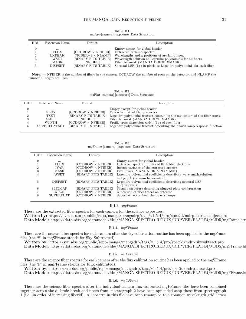
The MaNGA Data Reduction Pipeline 31

Table B1mgArc-[camera]-[exposure] Data Structure

HDU Extension Name Format Description

0 ... ... Empty except for global header1 FLUX [CCDROW × NFIBER] Extracted arclamp spectra2 LXPEAK [NFIBER+1 × NLAMP] Wavelengths and x positions of arc lamp lines.3 WSET [BINARY FITS TABLE] Wavelength solution as Legendre polynomials for all fibers4 MASK [NFIBER] Fiber bit mask (MANGA DRP2PIXMASK)5 DISPSET [BINARY FITS TABLE] Spectral LSF (1σ) in pixels as Legendre polynomials for each fiber

Note. — NFIBER is the number of fibers in the camera, CCDROW the number of rows on the detector, and NLAMP thenumber of bright arc lines.

Table B2mgFlat-[camera]-[exposure] Data Structure

HDU Extension Name Format Description

0 ... ... Empty except for global header1 FLUX [CCDROW × NFIBER] Extracted flatfield lamp spectra2 TSET [BINARY FITS TABLE] Legendre polynomial traceset containing the x,y centers of the fiber traces3 MASK [NFIBER] Fiber bit mask (MANGA DRP2PIXMASK)4 WIDTH [CCDROW × NFIBER] Profile cross-dispersion width (1σ) of each fiber5 SUPERFLATSET [BINARY FITS TABLE] Legendre polynomial traceset describing the quartz lamp response function

Table B3mgFrame-[camera]-[exposure] Data Structure

HDU Extension Name Format Description

0 ... ... Empty except for global header1 FLUX [CCDROW × NFIBER] Extracted spectra in units of flatfielded electrons2 IVAR [CCDROW × NFIBER] Inverse variance of the extracted spectra3 MASK [CCDROW × NFIBER] Pixel mask (MANGA DRP2PIXMASK)4 WSET [BINARY FITS TABLE] Legendre polynomial coefficients describing wavelength solution

in log10 A (vacuum heliocentric)5 DISPSET [BINARY FITS TABLE] Legendre polynomial coefficients describing spectral LSF

(1σ) in pixels6 SLITMAP [BINARY FITS TABLE] Slitmap structure describing plugged plate configuration7 XPOS [CCDROW × NFIBER] X position of fiber traces on detector8 SUPERFLAT [CCDROW × NFIBER] Superflat vector from the quartz lamps

B.1.3. mgFrame

These are the extracted fiber spectra for each camera for the science exposures.Written by: https://svn.sdss.org/public/repo/manga/mangadrp/tags/v1 5 4/pro/spec2d/mdrp extract object.proData Model: https://data.sdss.org/datamodel/files/MANGA SPECTRO REDUX/DRPVER/PLATE4/MJD5/mgFrame.html

B.1.4. mgSFrame

These are the science fiber spectra for each camera after the sky subtraction routine has been applied to the mgFramefiles (the ‘S’ in mgSFrame stands for Sky Subtracted).

Written by: https://svn.sdss.org/public/repo/manga/mangadrp/tags/v1 5 4/pro/spec2d/mdrp skysubtract.proData Model: https://data.sdss.org/datamodel/files/MANGA SPECTRO REDUX/DRPVER/PLATE4/MJD5/mgSFrame.html

B.1.5. mgFFrame

These are the science fiber spectra for each camera after the flux calibration routine has been applied to the mgSFramefiles (the ‘F’ in mgFFrame stands for Flux calibrated).

Written by: https://svn.sdss.org/public/repo/manga/mangadrp/tags/v1 5 4/pro/spec2d/mdrp fluxcal.proData Model: https://data.sdss.org/datamodel/files/MANGA SPECTRO REDUX/DRPVER/PLATE4/MJD5/mgFFrame.html

B.1.6. mgCFrame

These are the science fiber spectra after the individual-camera flux calibrated mgFFrame files have been combinedtogether across the dichroic break and fibers from spectrograph 2 have been appended atop those from spectrograph1 (i.e., in order of increasing fiberid). All spectra in this file have been resampled to a common wavelength grid across

32 Law et al.

Table B4mgSFrame-[camera]-[exposure] Data Structure

HDU Extension Name Format Description

0 ... ... Empty except for global header1 FLUX [CCDROW × NFIBER] Sky-subtracted spectra in units of flatfielded electrons2 IVAR [CCDROW × NFIBER] Inverse variance of the sky-subtracted spectra3 MASK [CCDROW × NFIBER] Pixel mask (MANGA DRP2PIXMASK)4 WSET [BINARY FITS TABLE] Legendre polynomial coefficients describing wavelength solution

in log10 A (vacuum heliocentric)5 DISPSET [BINARY FITS TABLE] Legendre polynomial coefficients describing spectral LSF

(1σ) in pixels6 SLITMAP [BINARY FITS TABLE] Slitmap structure describing plugged plate configuration7 XPOS [CCDROW × NFIBER] X position of fiber traces on detector8 SUPERFLAT [CCDROW × NFIBER] Superflat vector from the quartz lamps9 SKY [CCDROW × NFIBER] Subtracted model sky spectra in units of flatfielded electrons

Table B5mgFFrame-[camera]-[exposure] Data Structure

HDU Extension Name Format Description

0 ... ... Empty except for global header1 FLUX [CCDROW × NFIBER] Flux calibrated spectra in units of 10−17 erg s−1 cm−2 A−1 fiber−1

2 IVAR [CCDROW × NFIBER] Inverse variance of the flux-calibrated spectra3 MASK [CCDROW × NFIBER] Pixel mask (MANGA DRP2PIXMASK)4 WSET [BINARY FITS TABLE] Legendre polynomial coefficients describing wavelength solution

in log10 A (vacuum heliocentric)5 DISPSET [BINARY FITS TABLE] Legendre polynomial coefficients describing spectral LSF

(1σ) in pixels6 SLITMAP [BINARY FITS TABLE] Slitmap structure describing plugged plate configuration7 XPOS [CCDROW × NFIBER] X position of fiber traces on detector8 SUPERFLAT [CCDROW × NFIBER] Superflat vector from the quartz lamps9 SKY [CCDROW × NFIBER] Subtracted model sky spectra in units of 10−17 erg s−1 cm−2 A−1 fiber−1

Table B6mgCFrame-[exposure] Data Structure

HDU Extension Name Format Description

0 ... ... Empty except for global header1 FLUX [NWAVE × NFIBER] Camera combined, resampled spectra in units of 10−17 erg s−1 cm−2 Ang−1 fiber−1

2 IVAR [NWAVE × NFIBER] Inverse variance of the camera-combined spectra3 MASK [NWAVE × NFIBER] Pixel mask (DRP2PIXMASK)4 WAVE [NWAVE] Wavelength vector in units of A(vacuum heliocentric)5 DISP [NWAVE × NFIBER] Spectral resolution (1σ LSF) in units of A6 SLITMAP [BINARY FITS TABLE] Slitmap structure describing plugged plate configuration9 SKY [NWAVE × NFIBER] Resampled model sky spectra in units of 10−17 erg s−1 cm−2 Ang−1 fiber−1

Note. — Both LINEAR and LOG format versions of this file are produced, with either logarithmic or linear wavelength sampling respectively.NWAVE is the total number of wavelength channels (6732 for LINEAR, 4563 for LOG). NFIBER = 1423 total fibers.

the entire MaNGA survey using a basis spline technique described in §7 (the ‘C’ in mgCFrame stands for Calibratedand Camera Combined on a Common wavelength grid). There are two versions of this file; the first uses a logarithmicwavelength sampling from log10(λ/A)=3.5589 to 4.0151 (NWAVE=4563 spectral elements). The second uses a linearwavelength sampling running from 3622.0 to 10353.0 A (NWAVE=6732 spectral elements).

Written by: https://svn.sdss.org/public/repo/manga/mangadrp/tags/v1 5 4/pro/spec2d/mdrp combinecameras.proData Model: https://data.sdss.org/datamodel/files/MANGA SPECTRO REDUX/DRPVER/PLATE4/MJD5/mgCFrame.html

B.2. Final DRP data products

Depending on the science case, different final summary products are desirable. The MaNGA DRP provides bothRSS files and regularly-gridded combined data cubes, with both logarithmic and linear wavelength solutions.

These have the naming convention of manga-[PLATEID]-[IFUDESIGN]-[BIN][MODE].fits.gz. PLATEIDrefers to the four or five digit plate identifer. IFUDESIGN refers to the design id of the IFU bundle. BIN refers to thewavelength sampling of the output data product, LOG for logarithmic sampling, or LIN for linear sampling. MODE

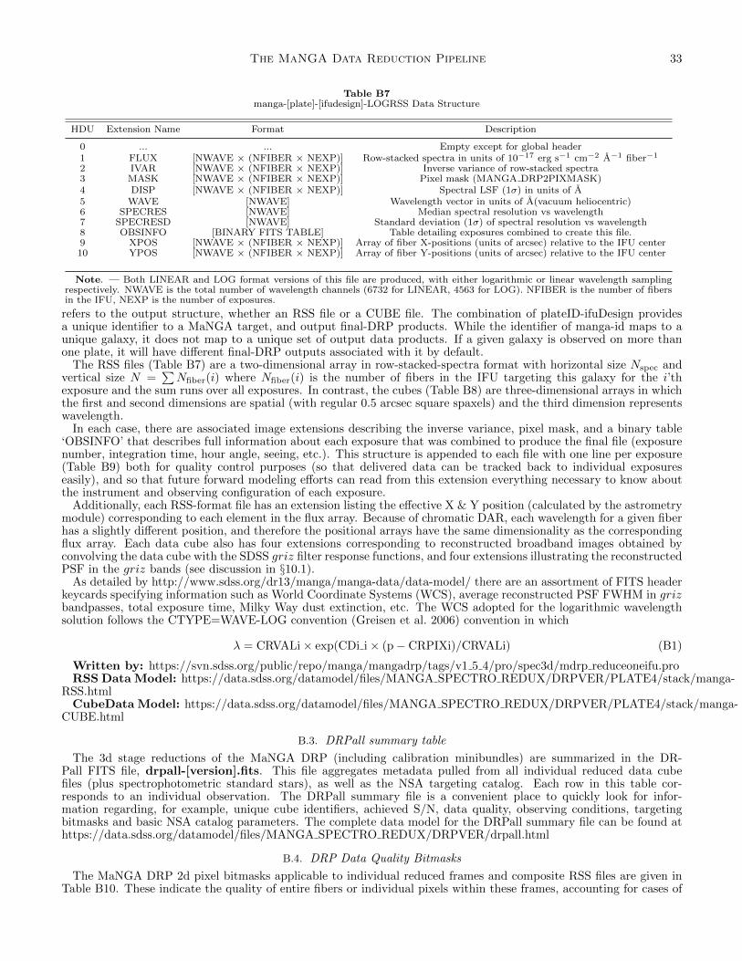
The MaNGA Data Reduction Pipeline 33

Table B7manga-[plate]-[ifudesign]-LOGRSS Data Structure

HDU Extension Name Format Description

0 ... ... Empty except for global header1 FLUX [NWAVE × (NFIBER × NEXP)] Row-stacked spectra in units of 10−17 erg s−1 cm−2 A−1 fiber−1

2 IVAR [NWAVE × (NFIBER × NEXP)] Inverse variance of row-stacked spectra3 MASK [NWAVE × (NFIBER × NEXP)] Pixel mask (MANGA DRP2PIXMASK)4 DISP [NWAVE × (NFIBER × NEXP)] Spectral LSF (1σ) in units of A5 WAVE [NWAVE] Wavelength vector in units of A(vacuum heliocentric)6 SPECRES [NWAVE] Median spectral resolution vs wavelength7 SPECRESD [NWAVE] Standard deviation (1σ) of spectral resolution vs wavelength8 OBSINFO [BINARY FITS TABLE] Table detailing exposures combined to create this file.9 XPOS [NWAVE × (NFIBER × NEXP)] Array of fiber X-positions (units of arcsec) relative to the IFU center10 YPOS [NWAVE × (NFIBER × NEXP)] Array of fiber Y-positions (units of arcsec) relative to the IFU center

Note. — Both LINEAR and LOG format versions of this file are produced, with either logarithmic or linear wavelength samplingrespectively. NWAVE is the total number of wavelength channels (6732 for LINEAR, 4563 for LOG). NFIBER is the number of fibersin the IFU, NEXP is the number of exposures.

refers to the output structure, whether an RSS file or a CUBE file. The combination of plateID-ifuDesign providesa unique identifier to a MaNGA target, and output final-DRP products. While the identifier of manga-id maps to aunique galaxy, it does not map to a unique set of output data products. If a given galaxy is observed on more thanone plate, it will have different final-DRP outputs associated with it by default.

The RSS files (Table B7) are a two-dimensional array in row-stacked-spectra format with horizontal size Nspec andvertical size N =

∑Nfiber(i) where Nfiber(i) is the number of fibers in the IFU targeting this galaxy for the i’th

exposure and the sum runs over all exposures. In contrast, the cubes (Table B8) are three-dimensional arrays in whichthe first and second dimensions are spatial (with regular 0.5 arcsec square spaxels) and the third dimension representswavelength.

In each case, there are associated image extensions describing the inverse variance, pixel mask, and a binary table‘OBSINFO’ that describes full information about each exposure that was combined to produce the final file (exposurenumber, integration time, hour angle, seeing, etc.). This structure is appended to each file with one line per exposure(Table B9) both for quality control purposes (so that delivered data can be tracked back to individual exposureseasily), and so that future forward modeling efforts can read from this extension everything necessary to know aboutthe instrument and observing configuration of each exposure.

Additionally, each RSS-format file has an extension listing the effective X & Y position (calculated by the astrometrymodule) corresponding to each element in the flux array. Because of chromatic DAR, each wavelength for a given fiberhas a slightly different position, and therefore the positional arrays have the same dimensionality as the correspondingflux array. Each data cube also has four extensions corresponding to reconstructed broadband images obtained byconvolving the data cube with the SDSS griz filter response functions, and four extensions illustrating the reconstructedPSF in the griz bands (see discussion in §10.1).

As detailed by http://www.sdss.org/dr13/manga/manga-data/data-model/ there are an assortment of FITS headerkeycards specifying information such as World Coordinate Systems (WCS), average reconstructed PSF FWHM in grizbandpasses, total exposure time, Milky Way dust extinction, etc. The WCS adopted for the logarithmic wavelengthsolution follows the CTYPE=WAVE-LOG convention (Greisen et al. 2006) convention in which

λ = CRVALi× exp(CDi i× (p− CRPIXi)/CRVALi) (B1)

Written by: https://svn.sdss.org/public/repo/manga/mangadrp/tags/v1 5 4/pro/spec3d/mdrp reduceoneifu.proRSS Data Model: https://data.sdss.org/datamodel/files/MANGA SPECTRO REDUX/DRPVER/PLATE4/stack/manga-

RSS.htmlCubeData Model: https://data.sdss.org/datamodel/files/MANGA SPECTRO REDUX/DRPVER/PLATE4/stack/manga-

CUBE.html

B.3. DRPall summary table

The 3d stage reductions of the MaNGA DRP (including calibration minibundles) are summarized in the DR-Pall FITS file, drpall-[version].fits. This file aggregates metadata pulled from all individual reduced data cubefiles (plus spectrophotometric standard stars), as well as the NSA targeting catalog. Each row in this table cor-responds to an individual observation. The DRPall summary file is a convenient place to quickly look for infor-mation regarding, for example, unique cube identifiers, achieved S/N, data quality, observing conditions, targetingbitmasks and basic NSA catalog parameters. The complete data model for the DRPall summary file can be found athttps://data.sdss.org/datamodel/files/MANGA SPECTRO REDUX/DRPVER/drpall.html

B.4. DRP Data Quality Bitmasks

The MaNGA DRP 2d pixel bitmasks applicable to individual reduced frames and composite RSS files are given inTable B10. These indicate the quality of entire fibers or individual pixels within these frames, accounting for cases of

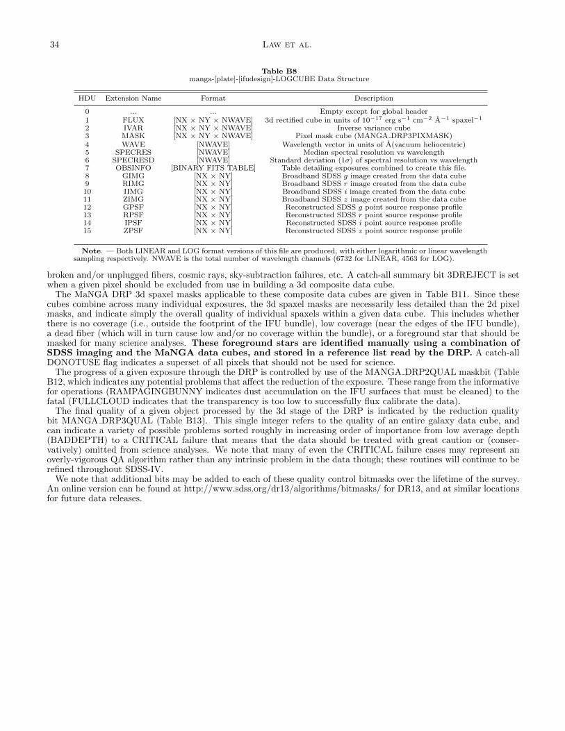
34 Law et al.

Table B8manga-[plate]-[ifudesign]-LOGCUBE Data Structure

HDU Extension Name Format Description

0 ... ... Empty except for global header1 FLUX [NX × NY × NWAVE] 3d rectified cube in units of 10−17 erg s−1 cm−2 A−1 spaxel−1

2 IVAR [NX × NY × NWAVE] Inverse variance cube3 MASK [NX × NY × NWAVE] Pixel mask cube (MANGA DRP3PIXMASK)4 WAVE [NWAVE] Wavelength vector in units of A(vacuum heliocentric)5 SPECRES [NWAVE] Median spectral resolution vs wavelength6 SPECRESD [NWAVE] Standard deviation (1σ) of spectral resolution vs wavelength7 OBSINFO [BINARY FITS TABLE] Table detailing exposures combined to create this file.8 GIMG [NX × NY] Broadband SDSS g image created from the data cube9 RIMG [NX × NY] Broadband SDSS r image created from the data cube10 IIMG [NX × NY] Broadband SDSS i image created from the data cube11 ZIMG [NX × NY] Broadband SDSS z image created from the data cube12 GPSF [NX × NY] Reconstructed SDSS g point source response profile13 RPSF [NX × NY] Reconstructed SDSS r point source response profile14 IPSF [NX × NY] Reconstructed SDSS i point source response profile15 ZPSF [NX × NY] Reconstructed SDSS z point source response profile

Note. — Both LINEAR and LOG format versions of this file are produced, with either logarithmic or linear wavelengthsampling respectively. NWAVE is the total number of wavelength channels (6732 for LINEAR, 4563 for LOG).

broken and/or unplugged fibers, cosmic rays, sky-subtraction failures, etc. A catch-all summary bit 3DREJECT is setwhen a given pixel should be excluded from use in building a 3d composite data cube.

The MaNGA DRP 3d spaxel masks applicable to these composite data cubes are given in Table B11. Since thesecubes combine across many individual exposures, the 3d spaxel masks are necessarily less detailed than the 2d pixelmasks, and indicate simply the overall quality of individual spaxels within a given data cube. This includes whetherthere is no coverage (i.e., outside the footprint of the IFU bundle), low coverage (near the edges of the IFU bundle),a dead fiber (which will in turn cause low and/or no coverage within the bundle), or a foreground star that should bemasked for many science analyses. These foreground stars are identified manually using a combination ofSDSS imaging and the MaNGA data cubes, and stored in a reference list read by the DRP. A catch-allDONOTUSE flag indicates a superset of all pixels that should not be used for science.

The progress of a given exposure through the DRP is controlled by use of the MANGA DRP2QUAL maskbit (TableB12, which indicates any potential problems that affect the reduction of the exposure. These range from the informativefor operations (RAMPAGINGBUNNY indicates dust accumulation on the IFU surfaces that must be cleaned) to thefatal (FULLCLOUD indicates that the transparency is too low to successfully flux calibrate the data).

The final quality of a given object processed by the 3d stage of the DRP is indicated by the reduction qualitybit MANGA DRP3QUAL (Table B13). This single integer refers to the quality of an entire galaxy data cube, andcan indicate a variety of possible problems sorted roughly in increasing order of importance from low average depth(BADDEPTH) to a CRITICAL failure that means that the data should be treated with great caution or (conser-vatively) omitted from science analyses. We note that many of even the CRITICAL failure cases may represent anoverly-vigorous QA algorithm rather than any intrinsic problem in the data though; these routines will continue to berefined throughout SDSS-IV.

We note that additional bits may be added to each of these quality control bitmasks over the lifetime of the survey.An online version can be found at http://www.sdss.org/dr13/algorithms/bitmasks/ for DR13, and at similar locationsfor future data releases.

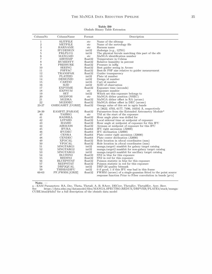
The MaNGA Data Reduction Pipeline 35

Table B9ObsInfo Binary Table Extension

ColumnNo ColumnName Format Description

1 SLITFILE str Name of the slitmap2 METFILE str Name of the metrology file3 HARNAME str Harness name4 IFUDESIGN int32 ifudesign (e.g., 12701)5 FRLPLUG int16 The physical ferrule matching this part of the slit6 MANGAID str MaNGA identification number7 AIRTEMP float32 Temperature in Celsius8 HUMIDITY float32 Relative humidity in percent9 PRESSURE float32 Pressure in inHg10 SEEING float32 Best guider seeing in Arcsec11 PSFFAC float32 Best-fit PSF size relative to guider measurement12 TRANSPAR float32 Guider transparency13 PLATEID int32 Plate id number14 DESIGNID int32 Design id number15 CARTID int16 Cart id number16 MJD int32 MJD of observation17 EXPTIME float32 Exposure time (seconds)18 EXPNUM str Exposure number19 SET int32 Which set this exposure belongs to20 MGDPOS str MaNGA dither position (NSEC)21 MGDRA float32 MaNGA dither offset in RA (arcsec)22 MGDDEC float32 MaNGA dither offset in DEC (arcsec)

23-27 OMEGASET [UGRIZ] float32 Omega value of this set in ugriz bandsat [3622, 4703, 6177, 7496, 10354] A, respectively

28-39 EAMFIT [PARAM] float32 Parameters from the Extended Astrometry Modulea

40 TAIBEG str TAI at the start of the exposure41 HADRILL float32 Hour angle plate was drilled for42 LSTMID float32 Local sidereal time at midpoint of exposure43 HAMID float32 Hour angle at midpoint of exposure for this IFU44 AIRMASS float32 Airmass at midpoint of exposure for this IFU45 IFURA float64 IFU right ascension (J2000)46 IFUDEC float64 IFU declination (J2000)47 CENRA float64 Plate center right ascension (J2000)48 CENDEC float64 Plate center declination (J2000)49 XFOCAL float32 Hole location in xfocal coordinates (mm)50 YFOCAL float32 Hole location in yfocal coordinates (mm)51 MNGTARG1 int32 manga target1 maskbit for galaxy target catalog52 MNGTARG2 int32 manga target2 maskbit for non-galaxy target catalog53 MNGTARG3 int32 manga target3 maskbit for ancillary target catalog54 BLUESN2 float32 SN2 in blue for this exposure55 REDSN2 float32 SN2 in red for this exposure56 BLUEPSTAT float32 Poisson statistic in blue for this exposure57 REDPSTAT float32 Poisson statistic in red for this exposure58 DRP2QUAL int32 DRP-2d quality bitmask59 THISBADIFU int32 0 if good, 1 if this IFU was bad in this frame

60-63 PF FWHM [GRIZ] float32 FWHM (arcsec) of a single-gaussian fitted to the point sourceresponse function Prior to Fiber convolution in bands [griz]

Note. —a - EAM Parameters: RA, Dec, Theta, Theta0, A, B, RAerr, DECerr, ThetaErr, Theta0Err, Aerr, Berr.See https://data.sdss.org/datamodel/files/MANGA SPECTRO REDUX/DRPVER/PLATE4/stack/manga-CUBE.html#hdu7 for a full description of the obsinfo data model

36 Law et al.

Table B10MANGA DRP2PIXMASK Data Quality Bits

Bit Value Label Description

Mask bits per fiber0 1 NOPLUG Fiber not listed in plugmap file1 2 BADTRACE Bad trace2 4 BADFLAT Low counts in fiberflat3 8 BADARC Bad arc solution4 16 MANYBADCOLUMNS More than 10% of pixels are bad columns5 32 MANYREJECTED More than 10% of pixels are rejected in extraction6 64 LARGESHIFT Large spatial shift between flat and object position7 128 BADSKYFIBER Sky fiber shows extreme residuals8 256 NEARWHOPPER Within 2 fibers of a whopping fiber (exclusive)9 512 WHOPPER Whopping fiber, with a very bright source.

10 1024 SMEARIMAGE Smear available for red and blue cameras11 2048 SMEARHIGHSN S/N sufficient for full smear fit12 4096 SMEARMEDSN S/N only sufficient for scaled median fit13 8192 DEADFIBER Broken fiber according to metrology files

Mask bits per pixel15 32768 BADPIX Pixel flagged in badpix reference file.16 65536 COSMIC Pixel flagged as cosmic ray.17 131072 NEARBADPIXEL Bad pixel within 3 pixels of trace.18 262144 LOWFLAT Flat field less than 0.519 524288 FULLREJECT Pixel fully rejected in extraction model fit (INVVAR=0)20 1048576 PARTIALREJECT Some pixels rejected in extraction model fit21 2097152 SCATTEREDLIGHT Scattered light significant22 4194304 CROSSTALK Cross-talk significant23 8388608 NOSKY Sky level unknown at this wavelength (INVVAR=0)24 16777216 BRIGHTSKY Sky level > flux + 10∗(flux err) AND sky > 1.25 ∗ median(sky,99 pixels)25 33554432 NODATA No data available in combine B-spline (INVVAR=0)26 671108864 COMBINEREJ Rejected in combine B-spline27 134217728 BADFLUXFACTOR Low flux-calibration or flux-correction factor28 268435456 BADSKYCHI Relative chi2 > 3 in sky residuals at this wavelength29 536870912 REDMONSTER Contiguous region of bad chi2 in sky residuals (with threshold of relative chi2 > 3).30 1073741824 3DREJECT Used in RSS file, indicates should be rejected when making 3D cube

Note. —

Table B11MANGA DRP3PIXMASK Data Quality Bits

Bit Value Label Description

0 1 NOCOV No coverage in cube1 2 LOWCOV Low coverage depth in cube2 4 DEADFIBER Major contributing fiber is dead3 8 FORESTAR Foreground star

10 1024 DONOTUSE Do not use this spaxel for science

Note. —

Table B12MANGA DRP2QUAL Data Quality Bits

Bit Value Label Description

0 1 VALIDFILE File is valid1 2 EXTRACTBAD Many bad values in extracted frame2 4 EXTRACTBRIGHT Extracted spectra abnormally bright3 8 LOWEXPTIME Exposure time less than 10 minutes4 16 BADIFU One or more IFUs missing/bad in this frame5 32 HIGHSCAT High scattered light levels6 64 SCATFAIL Failure to correct high scattered light levels7 128 BADDITHER Bad dither location information8 256 ARCFOCUS Bad focus on arc frames9 512 RAMPAGINGBUNNY Rampaging dust bunnies in IFU flats

10 1024 SKYSUBBAD Bad sky subtraction11 2048 SKYSUBFAIL Failed sky subtraction12 4096 FULLCLOUD Completely cloudy exposure13 8192 BADFLEXURE Abnormally high flexure LSF correction

Note. —

The MaNGA Data Reduction Pipeline 37

Table B13MANGA DRP3QUAL Data Quality Bits

Bit Value Label Description

0 1 VALIDFILE File is valid1 2 BADDEPTH IFU does not reach target depth2 4 SKYSUBBAD Bad sky subtraction in one or more frames3 8 HIGHSCAT High scattered light in one or more frames4 16 BADASTROM Bad astrometry in one or more frames5 32 VARIABLELSF LSF varies significantly between component spectra6 64 BADOMEGA Omega greater than threshhold in one or more sets7 128 BADSET One or more sets are bad8 256 BADFLUX Bad flux calibration9 512 BADPSF PSF estimate may be bad

30 1073741824 CRITICAL Critical failure in one or more frames

Note. —