prediction-accuracy - pnas · cinsteetunet integre/-blochs /) asid q) s-oe the oecse,1,e1r...

GENETICS: H. H. LAUGHLIN

Wistar Institute in consultation with Castle, who has formulated thisreport.

1 See also Proc. Nat. Acad. Sci., 21, 390-399 (1935).2 King, H. D., Jour. Mammology, 17, 157-163 (1936).' Castle, W. E., Genetics and Eugenics, 4th Ed., 234 (1930).

THE COEFFICIENT OF PREDICTION-ACCURACY

Computation of the Portion ofIndividual Cases Common to Both the ParticularPrediction-Distribution and to the Subsequently Determined Actual-Distribu-

tion of the Same Measured and Counted PhenomenaBy HARRY H. LAUGHLIN

EUGENICS RECORD OFFICE, CARNEGIE INSTITUTION OF WASHINGTON, COLD SPRINGHARBOR, LONG ISLAND, N. Y.

Communicated January 4, 1937

Consider first the specifications for a sound formula for the coefficient ofprediction-accuracy. Regardless of how, where or why we got it, if wehave in hand a prediction in terms of a probability-distribution, and if thesubsequently determined actual-distribution corresponds exactly with theprediction-distribution, it is evident that the particular prediction is per-fect, and that consequently the coefficient of prediction-accuracy shouldequal 1.000. If, in another case, there be no overlapping of the two proba-bility-distributions (that is, if the subsequently determined actual-distri-bution does not overlap to any degree with the given prediction-distributionwhich is being tested), then the coefficient of prediction-accuracy shouldwork out in the value 0.000. If, in still another case, 95 per cent of theindividual values actually found were as predicted, then the coefficient ofprediction-accuracy should register 0.9500. And so on, if three-fourths orif one-half of the case values are common between the prediction-distribu-tion and the actual-distribution, then the nature of the coefficient of pre-diction-accuracy should be such that its formula would produce measuredcoefficients respectively of 0.7500 and of 0.5000. Thus the CPA is prop-erly measured by that portion of cases common to both areas "p" and "a."

Also both the particular prediction-basis and the subsequent actualcheck-up by first-hand survey, must be plotted in the same coordinateframe, in which K = f(R), in which R equals the measure of subject-quality and K equals the probability-value. Also each distribution-area(that is, "p" the prediction-area and "a" the actual area) must equal 1.000.Whenever any two normal probability-curves, each of which bounds an

area which equals 1.000, are plotted within the same coordinate frame (as

PROC. N. A. S.60

GENETICS: H. H. LA UGHLIN

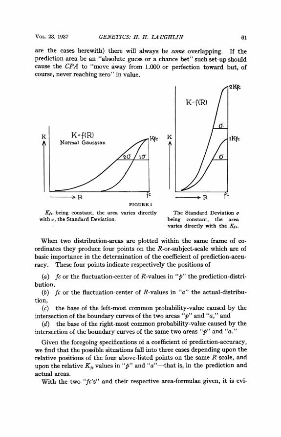
are the cases herewith) there will always be some overlapping. If theprediction-area be an "absolute guess or a chance bet" such set-up shouldcause the CPA to "move away from 1.000 or perfection toward but, ofcourse, never reaching zero" in value.

I2Kf

K=f(R)

K f_|R xf Kf.la CT~~

PIR fc R fKCFIGURE 1

KJC being constant, the area varies directly The Standard Deviation awith a, the Standard Deviation. being constant, the area

varies directly with the Kf,.

When two distribution-areas are plotted within the same frame of co-ordinates they produce four points on the R-or-subject-scale which are ofbasic importance in the determination of the coefficient of prediction-accu-racy. These four points indicate respectively the positions of

(a) fc or the fluctuation-center of R-values in "p" the prediction-distri-bution,

(b) fc or the fluctuation-center of R-values in "a" the actual-distribu-tion,

(c) the base of the left-most common probability-value caused by theintersection of the boundary curves of the two areas "p" and "a," and

(d) the base of the right-most common probability-value caused by theintersection of the boundary curves of the same two areas "p" and "a."

Given the foregoing specifications of a coefficient of prediction-accuracy,we find that the possible situations fall into three cases depending upon therelative positions of the four above-listed points on the same R-scale, andupon the relative Kr, values in "p" and "a"-that is, in the prediction andactual areas.With the two "fc's" and their respective area-formulae given, it is evi-

VOL. 23, 1937 61

GENETICS: H. H. LAUGHLIN PRoc. N. A. S.

THE COEFCIENT OF PREDICTION-ACCURACY (CPA)THE PORTION OF CASES COMMON TO BOTh THE PARTICULAR PREDICTION-DISTRIBUTION AND ITS

SUBSEQUENT ACTUAL-DISTRIBUTION OF MEASURED AND COUNTED PHENOMENA.CASE I.with Example-.

(a) TSe total Prediclion-area and the to/al Ac/al-area each tlooo. Each is plottedwilh/r the same codrdi?nae frame. - Ihe Same K, Mat dIke jame friequency or Probability-scale, and Ihe same R-class measure of the common sm/ect.I R-c/oas-ranre -1 R-unit. I Area-unit ==.o K by I R.

(b) 7y-pe a/each area-bounding carve, K=K E''Each curve wi/lu constant Xjs. andwek its Iwo C etlher equal to or adifferent from each other, but alwayste + 01 - 2 = C7 symmetrical.

(C) TwoC*maon Probability-values, due to overlapping of curmets Wp'and 'a, onecK to the left of baoh fcp and fca. the olher cK to Ike right of ba/h fcpr and fc a.

(d) Under the oarf/ular probabikify -curve, whether symmetrical orskew-edcArea to/efI f Area torkiAt fc=C q when f3/al Arza=L.ooa.Area to the left of fe. -a,- Area to/he right of fc= -9vj--

(e) C. PA sZ roaur constituent Tnrtegral-b-ocks. rio for Area wi/lth greater Kfj, one in eachof its lower extremities, (j K, and ®/) 'I and to forfAra wi/h lesser Kfc, in its

cenlral rei9onb, ®/ and

GIVEN Prediction-Arame.ooooI fep at point 15.75 can R-scale

t 5 fap a0. 1 25 pt K-scakic-o__ffp = 3.324 5 R -unl ts _I0- r_--CIy = 3.6.342 R-llnif5l

GIVEN Actual _teaIe.S.oppA_caa pent 20.00 oR-scale

Kfca 0. 0750 onK-scale_P___iGa = 4.9868 R-units__a - 6.6490 R- unitSa 3.3245 R- units

LEGFN K' Probobility fc = flealon-scMe r C-shtamia,de-l d,-i.fsi sy--.tiisIKile 41- r pr6bajLy- esieR' Measured S.bjet-q/lhy t a lft of particular fe -t .h. p-absbddy-ct-e I! n 0 t Wth p ead a.p.a p-pey ofPradlctW,-o-rea A rcghf of psr-lot.r fc -i. -rtaib. d eKRa -spcahispngdi-rqt-moa. p-operly ifAd./I-avca Kfl ' pr*bIlytyst/e,itprisclare-fcs e + 0, = 24&,-I-,otha- scanson obbsl-y.

FIND sWerssa. s tfsst *(fsp -fca/ is R-nifb.t fe pr-diccd-fc astual =g s 12502. (ea R-ocu4 a/sKi When /fcp,-cs / X'eon (fsa-cKmg/.ii,oJiiee or-the parhe a/ e/Xjby mceasr of/ ie o JsMdteneaa ema/seos

o KfspC( 'L - Kfsa C O7 The tw fo rehie fra the Coones PAhahshy at cKe, and®XtI 'X1,-g9 Zoc. cKe en R-scale 'iec.flps-dit/ar-Xe. X=4.59 R-units, Xe, a 5.84 R-i--s..etfocuo cKj a 18.750 -4.509 = 14.151 on the Rf-jasate

(b) R-l-cus of cWKhen (fca- e j zxtnandd lfcp -cKi /-Xs,, swe/etfor Miepaosrtse itof X h cn ef theofthe t melteimcaqi.c/r.ee.Q? KP *(.p c;U~: Kfc Ac 1-lo<fomue fer f Ce im on Pha hl i aftcK, a l7adU2 tlX, X,-g Zoecs cK, on R-scolo = loscus fC acl-Ifa + X,, X4= 1.98 R-unils, Xt, 3.23 R- unirls,/, The s-ca csKl = 20 000 + 1.984h 21 984 oen the R- s5we.

3. Wien Ate ftal amea odtes the parescelar s-robeliSehfc-csr-ve - 1.0000(a) Predsdion-area fe of fsp - 2 4r, - t + Or,) [02.--2 '.54961i/) Predkhoig-aaea f-eayt o fcp - 2 °4; (e or)-s.goo8-.o 2 4 0040ic) Actuea-area to coffca =24-Oe-(OT+Cj -l1.33335 ---266661 1

/d) Actual-area eo Lghf fe- 2O -,/e--i 2333414. The X01/s O/ C-Oeaet/ Ain/ysal-l-hsil (D ens' fro . eccataeIps_ dots-ac/ia--es-ca tih ahe_es -l,y, issan ef

Cinsteetunet Integre/-blochs /) asid Q) s-oe the oecse,1,e1r 4dsrihetia, -arma is-i/h /he lesser Kfc4 I 11 m nr

arlsh,n P.s-cde/ioesreccooe ./0 i3ep cKis460 R- 15.2 L 275 ---.(R5o-/sr ie O l.rh10 .r1/le44eCoZsnltcrAl-hih C/DQftp-cK5'3523R-ii'iti 1.07009 L,-s[.4504-r .r5s9so.o 85/.1262'Cbtstieens-vi-hleh hi

(6/When sic/sal- aes-e 1.0000 (S.fes e,{ *.5B hR-entr. .h8706-0l5--,-[/.5i05 i.5355/]'*.4140./eisStilentls/egs /-alhli 0i)ifcts-sc 98Rasi'- .5968 h, --'[.2247 0.6662]'. I4hCeons=iht/ enIe Acgsye/-blosA h

£: 4 Canaritectnt /elgs-i-hCOks-ijjFCFICIENT or PREDICTION ACCURACY (CPSI OG ven ielent relumhber ofe5/tndardm evafeions I-/ -qei ofAAe,fAsaei ralern#tas/aMe ca maeyAf,,/f6ekp fc.IPors-/cs ef ftael srnelmsicele es-a tsi/q pliessensu-mAr /5/ndeea`o,rd Dc-kc/aeo,.. (fr-n lied/c)WV7o/al Area,[l hnnctsel,ean hait ifa-lace yfcsen OT

62

PROPERTIES


dent that the first main step toward solution consists in locating the posi-tion, on the R-scale, of the foot of each common probability-value.The analytic geometry of the problem is developed by the three accom-

panying plates, one for each of the three cases. In each case the final solu-tion is reached by determining the area covered by the overlapping of theprediction-probability-distribution-area and the actual-probability-distri-bution-area.As above stated, the two areas being "compared-for-overlapping" must

be plotted in the same frame of coordinates, and in each case the totalarea under each of the two area-bounding curves must be equal to unity.Regardless of the number of cases upon which the particular distributionis based, said distribution must be reduced to percentages by R-classes sothat the total area under the particular bounding-curve is always equal to

1.0000. soooo__ rfc > K-~~~~K f(R)NNormal Gaussian

l.6e s --------------- Point of maximum

R \cR at one a from fc

FIGURE 2

The development of 0.6065 KX, as the K-point at which the Standard Deviation a

always crosses the K-scale.

1.000. This rule holds true for both the prediction-distribution and theactual-distribution--each must always equal 1.000. Beyond this specifica-tion for unity in extent the two areas and their bounding-curves may bevery different. Each curve may have its own fluctuation-center (fc), itsown highest probability-value (Kf,) and it may be skewed to any degreeto either the right or the left.The three cases, into which the possible types of the present problem

fall, run as follows:Case I is characterized by the set-up in which there are two common

probability-values. On the R-scale one common probability-value (cKl)lies below the two fluctuation-centers (fcp andfca), and the second commonprobability-value (cKr) lies above these two fluctuation-centers.

63VOL. 23, 1937

64 GENETICS: H. H. LA UGHLIN PROC. N. A. S.

CASE U.with Example.

PROPERTI ES (a) M9ie total Predction-area and the total Actua/-area each =1.0000. Each ti-p/oied within the same codrde>,ate frame. - the same K, that i the same Fvuencyor probability-scale, and the janme R-c/ass measure ef fhe common sabjede.

li-c/ass-range - I P-unit I Area-unit -.01 K by I R.(b) 9ype ofeac area-hounding curre, K = Kfe 0 Each carve with consant7 I4!. and

wtih Uts two 0 etfher equal to or different from oech oher, bues a/ways(Oj. + I)-2 - OsJymmetrical.

(C) ao eommon Probabiloty-valuej,due to over/a/ft?ing of curves p" and a either one'ckI to the left anrd the other cK, betweenthe two fCs p and a or cK. between thetwo fc3, and the other c&, to the r@to of botf fc s-

(d) inder the par/frular Probabhiliy- carve, whether symmetrial orasikewed,Area fo ft f(C Area to rg4ht fC O:0 when otalArea= 1.oaoo.Area (o/EefZC = and Area lo r4rht of fC - *e~

(e) C.PA.= r-7ree Constituent Itieyral-blocks. iwo for Area wi/h greater KRfc, in itslower exfremities, ®j(D and Cg) and one for Area wi/h lesser Kfs ©

GIVEN Prediction.Area=.oooo GIVEN Actual-Area -.0000fop at point 1500 on R-scale - -f.ca at point 20.00 on RI-sale

Kfcp = 0.1125 on 1-scale iI fca = 0.0750 on K-scaleto- (7s = 3.3245 R stls Cia - 4.9868 li-units. 1p 2.7448 R-unsits _Tea - 6.6490 R-unitsc8-~ _ 03.9042 R- units 3.3245 R.-units

S ti24 6 8 0 12 14 5 1 ii es2 4 16 2e 10 1i

LiQ.LrN2 HK Pr-obability fluoctation -ooniter 75 -standard devialien.sytinotricol cl, -like 1efIneat prnbaoilltysoaRl- Msosured SobJeotlquaSty 51 left of partclaors o Ieoe rneii/-s. is onoto Lath p and A.

pe-a propert ofPrdictionsvare t roightof partliclar fo -ia not ekeced i K0l- oerreopeoiding right -nolta* a properly efActual-area K(fs.probabilityo'taelum partiouler fo 0j o LT. 20j,nte.LoWk. pa-ti- coenioen probaLiMiy.

FiN fj prodaded -factual -.5.te sntteontlAo li-sceie. Zessis,o.t,. 9./pfoil-nt

li-(a orcoofwol(s-Kewen (fip-slio,) -Qe, lfca -rK,e,q1)-Xe, s5o/se/Li. ioeete 'alomY.e ofXe bymeansolhef/krimUio/neeseoujeoosnat

Xe-4.1R-wis, Xe-9.71lR-nfstitsThe torso c.j - -1-'-',4.71t on tei-eR ioale.

(A)RL- 6of s wshen (fp - _,,w)- f . sot r t i/ q n o ofh os

.sofe oAnse Comorz Predadt/--yat el-end(VX#-5-Xc,. Leeeosl4enRi-ssele.orso foaetsoi-Xt. X,.L.391i.stdsjX,,=361 Ri-onto.

7he torso csK4- 20.00 -i5.39 - 18.61 on3he R - srate.3. toen AiktK al area sfndr Ath par/tisular pro-eehueirty- ewre - 1.0000

(a)J e rea-, uto left of Cp2O. (Cr)fc25h3-s2 -L.41288lnee(ln) cfrenz.gca-aeatoco(A&toffp.-20a,s(Or,en ,)-I..1r4537- 2 - .5872acrActAai area/efl?toa9l fca -fc2Oren - 1.33333t 2 LL7610000pO_ l)Aciual -ae tfon iof fc0so-22 fh-(ae-J- .66667- .3333)

4 ao e toe,. ike Amne,o(f Comstent intogrei-hies (13 eat ® from the overriep,oi dislrbsteen--,amewith he rooaer- Ks.end of Cnsp*tcoent Integre.-Nes ® (runethle oerikejrng destribstr-area wi/k the iemer RI's

(a) etenPtrcdlrton-aoax - 1.0000 (f-su-4Ru.71= -snits1e.-71T5i C,-eL408-(Ato -.8256)] -.Ol 6oeocenloetmnft,ol-h/ci®fcp-oK5. 60li-snob. .9046.0 --[ M72-1.3004-1.1744)] - .2e86-Ceoon5ftivearrlo-kf.3f

(6) MM eAcual - area- I.0000 ®)fea-eclQ.19.71R-sntieit-1.4600 e1.(.4200 9.1.5-331-.s70fca-.-clSo. O.39li-onito. .2090Ose- -sC.0528.1.3333)..ll0a) -4601e- Ceoetonlfep1 -/eq2-h2o ©2

Su3 Cowsto/ent Inaereal-blok-s 0-7043 - COErrCJENT OFPRED1CTION-ACCURACYlCPA)

VC1-Okeneqstwo1ae/n/ooberoftodo.14rd DrrseienowIT.lLNsrurion2loeqosain/f oiaeael/lft/-o-igAtoslhoeomeo,syhre, offhoes-gi'sfX -Parttoe of total smeyoiorieol area ieibt.oedoe9 yhv-r num.ber of Stondoro DOeiatono. (Fwsno Tee)4V e i(a Arose. of Ameiooca,oCaon as/i ofZpanrk/asea irvon 0lK


In this case the coefficient of prediction-accuracy is equal to the summa-tion of four constituent integral-blocks as follows:

From that distribution-area with the greater K,..Block 1 = area between cc left and cKI.Block 2 = area between CKr and c right.

From that distribution-area with the lesser K,,.Block 3 = area between cKl and fc.Block 4 = area between fc and cKr.

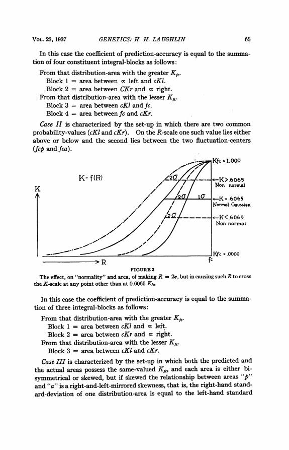
Case II is characterized by the set-up in which there are two commonprobability-values (cKl and cKr). On the R-scale one such value lies eitherabove or below and the second lies between the two fluctuation-centers(fcp and fca).

- , Kfc - 1.000

K= f(RI 41- / K>.6065K 7'// / Non rorral

} i / o~~~~~~/U4ft¢ -K=.6O65

1~~2Q ~ -KK.6065," / / /JNormal Gaussian

// /& C7t ~+K <.6065Non normal

KfcK .0000>R f'FIGURE 3

The effect, on "normality" and area, of making R = 2a, but in caulsing such R to crossthe K-scale at any point other than at 0.6065 Kfc.

In this case the coefficient of prediction-accuracy is equal to the summa-tion of three integral-blocks as follows:

From that distribution-area with the greater Kf,.Block 1 = area between cKI and cc left.Block 2 = area between cKr and x right.

From that distribution-area with the lesser Kf,.Block 3 = area between cKI and cKr.

Case III is characterized by the set-up in which both the predicted andthe actual areas possess the same-valued KJC, and each area is either bi-symmetrical or skewed, but if skewed the relationship between areas "p"and "a" is a right-and-left-mirrored skewness, that is, the right-hand stand-ard-deviation of one distribution-area is equal to the left-hand standard

VOL. 23, 1937 65

66

PROPERTIES

GIVEN PredictitAi- Wjp at ptuz-- KorpttdHg:

GENETICS: H. H. LA UGHLIN PNoC. N. A. S.

CASE mf.with Example.

(al-'h total Preditobn-a-rea and the to/at Actual-area each = 1.0000. Each plottedwilhin the same cooradinate frame the same K, that 6, te same Frequency or Pro-bability-scale, and the same R-c/as measure f tke common subject.I 2-cass-ranqe R-unit. I Area-an = .01 K by I R.

(b)iypeofeach areobonding curve, K- KfsEj o i Each curve we/h costafnt Kfc equalto i/e Kfc of the other curve, and with two CFl either equal to or differeeot from eachother, but always Oe+ 2 asymmetreal. If skewed, the two areas meas beskewed iz mirror-relation to each oaher' as case of the gioen example

(C) One common Phobabillty-value, due to overlappeo cl curarves p and "a'"Zf2r or tcKis always located midway between the two fc's ie. between fcp and fca.

d) Undet the particular praWbility-curve, wvhether rymmetric-al or skekhd,Area to left fe :Arma tortht fc = Q: When total area = I0oooo,Area fo lef, fc -&w Area to r4qht fc

(e) CPA. wo con5stitenft Tiotegral blocks, one for each prooahbi/iy-distribution-area.OD for area ith fc to right an fr area we/zA fc Ao left.

ion-A eaw-iOOOO GIVEN Actual-Area. i.ooo

oint 15.00 on R-scale - fca at point 20.00 on R-scalt0.0875 K-scale __ _ __ Kfca 0.0875 on K-scale

R-unin sa 4.5593 R-units4.2746 R- units -_ 4.8441 R-units-4.8441 R-unis 0, 4.2746 R-units

LEGEND K-Probabittly fcfT-liuation center ui.54a.rd dcviafionsy-u r-ical cKe.th.ieff-most probabiitty svaluR -Me.3ure-d Ssbject-qusity g a left f paruiculur fc -Is. we pmab.blity -cu. is oonns, to bota p *ssd ap a prop-ry of Pndiction-are. t sur ofht partlcuir fu -i.e. at nkeO.-d s-K, -the correspndi ng riqht - mouta ' property of Astuel- sae Kf-= prvbaWity sulue i pecrl.uarlfc 0 + LT = 2i5s,uwhen Cos- cornone probabilsty.

FIND cu.kloesoceiXe. lds-tufp-f;InlR-ut.1. fe predicted - fc actual - qg 5.002 R-Louo of sK when foen - cKI - x, and (fp -sK) =X, , sola fael the posilve value of Xt by moans oftae .snutameus eqcotioo

Kfp i - =Kfca hSe two forlautlapMoewomn Probabl/it at cK. andU2 X., - 9 -Xe locus _K on R-lscae - tocus fc redticeed + Xt X, - 2 50 R-un its Xe 2.50 R-unit..' - 7 e locu/s cK - 15.00 + Z. 50 - i7. 50

3. When It total area tader the particular prohabelity-curve - 1.0000(a Prediciion -area to left o fop - 21-(it + (7 .93754-2 :.4688 1 2oo0bi Prediction-area rLioht acffp 2tLT (CT,+O0I-1.06246-2 .5312 °C1 Actual- area to lta of fca - 2 a-I-i,( 4+a I.0626 2 - .53 1z 0000(di Actjual area.g oriLt of fca - 240t -i--(Ct4I- .93754 2 4.68J8°

4. The Value of the equal Conosiluent Integral-b locki (i and (23 frum the overlapping areuo of 'pr and 'a'= 1 - zi X IV

a) When Pnxieien-aroa 10000 (D fuP-cK2.50 fl-units .516f (5gp-o.5312-971,7t 1Ob251j53218=-C`ostiftsentlJntgilhost@(b) Whan Actual - area 1.0000 ( Fca-CK-2.5O R-units ..5161 e-re.-[53i2-(i1971 106259)i.24&CaonjtiluentIntegrol-ldockGD

tl2Cono{lenzl alneqral-blocks - P-C0 COETFICIENT O0PREDICTION-ACCURACY (C P.A)

* L . Given equisvaiene nurmbUr of Standard DtevinaPE r -C YN. - Numerical ogct-ralent of Ama eo the left or right, a the case may be, of the given fc.m - Portion of total symmetrzial area jsbtending glean member of eSiandard Dereioticns (from 7rehe,.TV . CStal Area, if symmeirical, on aoses of particuar given Cl


deviation of the second, and vice versa. In this case there is only onecommon probability-value and this is always midway between the twofluctuation-centers (fcp and fca).

In this case the coefficient of prediction-accuracy is equal to the summa-tion of two integral blocks-one from each of the two basic distribution-areas.

Block 1, from the distribution-area with the Kf, to the right, equals areabetween cK and x left.

Block 2, from the distribution-area with the Kr, to the left, equals areabetween cK and c right.The solution of these problems is made possible by use of the following

properties of the probability-distribution area, that is, of the area underthe Gaussian or normal curve of error:

(1) The first basic probability-formula for the symmetrical probability-area, in which K = class probability and R = class-range in subject-value,is

RsK = f(R) = Kcf.e2ac.

The value of the probability K may be continuous, but R, the measuredquality under consideration, must always be broken into a series of classesor grades.

a = the standard deviation, e = 2.7182 which is the base of the system ofnatural logarithms. fc is the fluctuation-center of R-values.

(2) The second basic formula for the symmetrical probability-distribu-tion area represents the value of the maximum ordinate as

Kf N

When distribution-data are given it is always possible to reduce the ab-solute number within each R-class to the percentage basis, and thus N, or

the total area, is made to equal 1.000.V/27r = 2.5066 is a constant, and when N is constant, KfC and or are in-

terchangeable and are inversely proportional to each other. If KJ, beconstant N or total area varies directly with a, or if a be constant N variesdirectly with Kfc. (See Fig. 1.)

(3) Regardless of the skewness of the particular distribution, graphi-cally the standard deviation crosses the Kf, at a K-point always equal to0.6065 times KJ,. This value is deduced as follows:

R'Given K = Kfce 2u5Let Kf, = 1.000 and let R =.

Then K 1-e-2' - =- = 0.6065 which is a constant. (See

Fig. 2.)

VOL. 23, 1937 67


(4) Further significance of the point 0.6065K on the maximum ordinate.This point 0.6065Kf, is the only point on the maximum ordinate at

which, if the KfC remain constant, the doubling of the R-value (in thiscase the a) will result in the exact doubling of the newly plotted distribu-tion-area. Thus, if R equal two original standard deviations, and if thepoint of maximum slope on the boundary curve be above 0.6065, the result-ing "non-normal" area will be more than doubled; if such point be below0.6065 the resulting area will be less than doubled-compared with theoriginal normal Gaussian area for which the standard deviation equals1.000. (See Fig. 3.)

Again, if the R-value of the original normal area be selected at less thanone standard deviation (graphically above 0.6065Kf,), and such R-valuebe doubled but kept at the same K-point (above 0.6065Kf,), the changecauses a new "non-normal" slope in the new boundary-curve-of-distribu-tion, and the new area will always be less than the original normal area inwhich the standard deviation equals 1.000.Or if the new R-value be greater than one standard deviation (graphi-

cally below 0.6065K,,) and such R-value be doubled, and the new "non-normal" area be plotted in the same manner as when the new standard de-viation is less than one, such new area will always be greater than theoriginal normal area in which the standard deviation equals 1.000. (SeeFig. 4.)Thus when the R-value = la, and the K value = 0.6065, all other fac-

tors remaining constant, such R-value is the only R-value, the doubling orother increase of which will cause a proportional increase in the normal dis-tribution-area.Next to the rectangle, the "normal-probability-distribution-area" is

probably the simplest flat geometric figure the area of which varies directlywith the change (that is, with the first power) of either one of its two co-ordinate factors, while the second remains constant. But there is this dif-ference: Plot any rectangle and any normal-probability-distribution-areaeach within an x-y frame of coordinates, the area of the rectangle variesdirectly with the value of x selected at any y-point, or with the value of yselected at any x-point; while the area of the normal-probability-distribu-tion-figure varies directly with x only when x equals the standard deviation(which always crosses the y-coordinate at the point equal to 0.6065 of themaximum ordinate), and directly with y only when y is the maximum ordi-nate, which always crosses the x-coordinate at the fluctuation-center of x-

values.(5) Relative areas. If the total normal distribution-area be 1.000, and

the Kf, be constant at 1K, then that portion of the area to the rightof the particular K,, is to that portion of the area to the left of said Kf, as

68 PROC. N. A. S.


the particular standard deviation right is to the particular standard devia-tion left.Area right: area left = art alft(6) Skewness. Using the second basic formula above given, we find

that, if the Kft be constant the area varies directly with the standard devia-tion in a symmetrical or non-skewed area. Now, if the area be skewed, ahypothetical area must be postulated temporarily. Let, for example, the"standard deviation symmetrical" (as) equal 0.50, then shift the "standarddeviation left" (a,) to the value of 0.55. Now if the Kr, be constant at1K, and the area be made symmetrical with the new a = 0.55, the newtotal postulated-area equals X in the ratio 1: 0.50 = X: 0.55, in which caseX = 1.10, i.e., the 0fleft would belong to a total area equal to 1.10 with itsa symmetrical at 0.55 and its Kf, constant at 1K-the original value.

Kfc -.0000

K- f(R.) /K > .6065K //i / fNon- normal

/ /J/ U <--K .6065X/ / 1Normal Gaussian

~~2RJ ~ I/ ~~~~~~~-K< .6065

/ / Non normal

Kfc-- .0000-,-~~~~~~~~~~~~~~~cR

FIGURE 4

The effect, on "normality" and area, of doubling the normal R-value at any pointon the K-scale other than at 0.6065 Kf,.

But actually the total area must remain constant at 1.000, and KJ,C mustremain constant at 1K. Then since the actual-skewed-area to the lefthas already consumed 0.55 of the total-actual-area, this leaves 0.45 for thearea to the right of K,,. Similarly computed the 0right would belong to anewly postulated symmetrical distribution represented by a total area

equal not to 1.000 but to 0.90, and with Kf, constant at the same 1Kvalue.

Therefore 2alsymmetrical = (f1eft + aright-(7) Down the long S-curve (one of which bounds the top side of the

probability-distribution to the left and another to the right of the particular

VOL. 23, 1937 69


K.,), beginning at the top, where the slope equals zero, and descending theslope increases continuously until the descent-point, located at. the heightof K at la removed from the particular fluctuation-center, is reached, i.e.,until the descent-value 0.6065K7,, is reached. This descent-point locatesalso the maximum slope of the long S-bounding-curve. (The greatness ofthis maximum slope is a function of its adjacent standard deviation a.)Therebelow the rapidity of descent decreases continuously, and for thelatter reason never reaches the level whereat K = 0, but theoreticallyextends indefinitely, continuously approaching but never attainingparallelism with the particular R-scale at K = 0.

(8) The total area under each curve (the prediction-area "p" and theactual-area "a") independently is equal to 1.000. The total area, includingthe overlap covered by both curves, equals (2 - CPA or overlap).The prediction-basis with the specifications listed in the earlier

paragraphs is the one actually used. The selection of the particular pre-diction-basis must, of course, be justified by the logic of the particular caseunder analysis, but how the particular prediction-basis was derived or whyused are matters which do not concern the basic theory of the coefficient ofprediction-accuracy nor the technique of its use. The prediction-basismay thus be a guess or an intuition; it may be based upon a single proba-bility-distribution composed of a few individual cases carelessly measured,or it may be based upon the probability-resultant of many constituentprobability-factors, each based upon many individual cases, and each ac-curately and confidently measured. An example of the latter type of pre-diction-basis is one produced by the probability-resultant* made by theproper synthesis of one cross-section from each of a number of selectedmanerkons each of which individually pictures mathematically the rela-tionship K = f(M, R), in which M is the particular prediction-basis, R isthe thing-predicted and K is the probability. The point is that, in thisparticular study, the prediction-basis is being tested for its accuracy, notfor its source.But in interpreting the meaning of a computed value for the coefficient

of prediction-accuracy, the situation is such that one can criticize usefullythe soundness of construction of the particular prediction-basis. It is evi-dent that if for many quantitative distribution-data on the same trait orquality, within the same population, the prediction-accuracy in many testsruns consistently high, there must be something besides luck or chancewhich favors the particular prediction-set-up. If the high running coeffi-cient of prediction-accuracy be based upon many independent factors, andeach, in turn, is composed of many carefully measured individual cases,then confidence is justified that the essential major factors are in hand andare properly weighted and coordinated in the given prediction-basis.But if the coefficient of prediction-accuracy run consistently low then,

70 PROC. N. A. S.

PHYSIOLOGY: W. J. CROZIER

regardless of how carefully the particular prediction-basis is computed,it indicates that some major factor or factors are omitted, or areimproperly weighted or coordinated, in the particular prediction-basis beingtested for accuracy.

In comparing two different prediction-bases against the same subsequentlydetermined set of actual distribution-values, the coefficient of prediction-accuracy tests the relative merit of these two prediction-bases as to theirrelative correctness in the inclusion of their own postulated constituentfactors, and in the relative weights and co6rdinations given such factors.

In any case in which one has in hand a prediction-basis in terms of aprobability-distribution, and has also in hand the actual subsequent orother independently secured measuring and counting of the same qualityin the same population, the coefficient of, prediction-accuracy (CPA)presents a sound formula for judging the given probability-distribution-production-basis as to its degree of success-no excuses taken.The next step in good research is, of course, to find out why the particular

prediction-basis which was actually used was not more successful.* H. H. Laughlin, "The Probability-resultant," Proc. Nat. Acad. Sci., 21, 11, 601-610

(1935).

STRENGTH-DURATION CURVES AND THE THEORY OFELECTRICAL EXCITATION

By W. J. CROZIER

BIOLOGIcAL LABORATORIES, HARVARD UNIVERSITY

Communicated December 22, 1936

I. An instructive parallel exists between measurements of electrical ex-citability, particularly for repetitive condenser discharges or constant cur-rent pulses, and the data of visual flicker. The comparison derives fromprobability considerations, and provides a means of analysis independentof any specific assumptions as to the physico-chemical character of theexcitation process.Numerous observations describe the general relationship between mag-

nitude of stimulating potential or current and the time for threshold excita-tion, particularly in nerve. It is well known that for a chosen degree ofexcitation the required current (or voltage) declines to an asymptotic levelas the exposure time is increased.' No fully satisfactory theory of theform of the strength-duration curve has been provided. From a rationalconception of the effects connected with electrical excitation Hill2 derivedequations describing rather closely the relation between current or poten-tial (C) and its duration (t) for constant response. It is not clear that this

VOL. 23, 1937 71

prediction-accuracy - pnas · cinsteetunet integre/-blochs /) asid q) s-oe the oecse,1,e1r...

Documents