Predicting Shale Production with Integrated Multi-Variate Statistics

Murray Roth

Transform Software and Services, Inc.

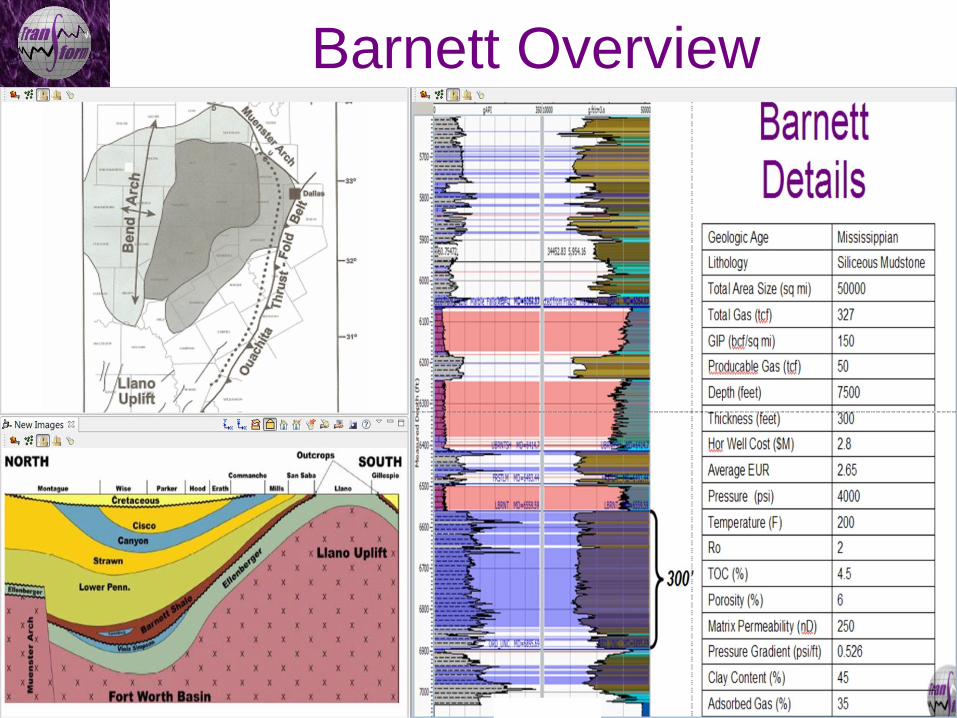
Barnett Overview

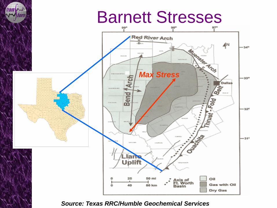
Barnett Stresses

Max Stress

Source: Texas RRC/Humble Geochemical Services

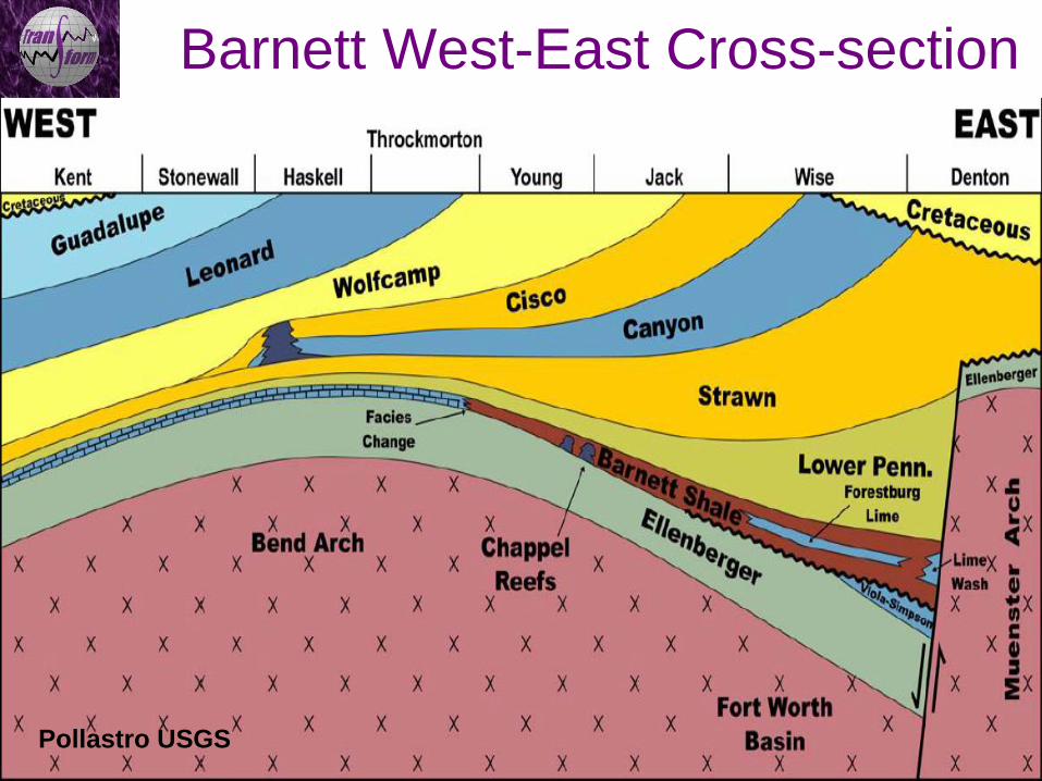
Barnett West-East Cross-section

Pollastro USGS

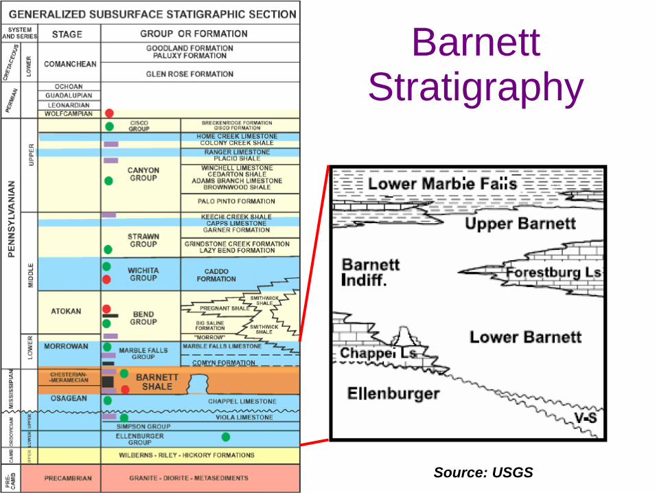
Barnett Stratigraphy

Source: USGS

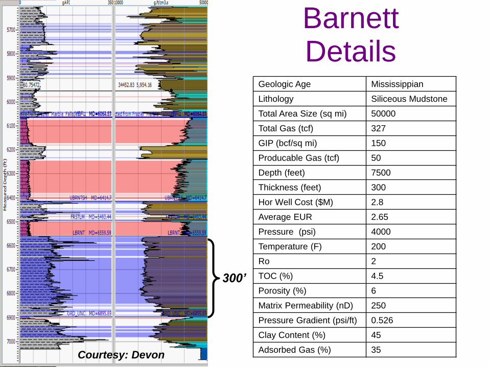
Barnett Details

Geologic Age Mississippian

Lithology Siliceous Mudstone

Total Area Size (sq mi) 50000

Total Gas (tcf) 327

GIP (bcf/sq mi) 150

Producable Gas (tcf) 50

Depth (feet) 7500

Thickness (feet) 300

Hor Well Cost ($M) 2.8

Average EUR 2.65

Pressure (psi) 4000

Temperature (F) 200

Ro 2

TOC (%) 4.5

Porosity (%) 6

Matrix Permeability (nD) 250

Pressure Gradient (psi/ft) 0.526

Clay Content (%) 45

Adsorbed Gas (%) 35

300’

Courtesy: Devon

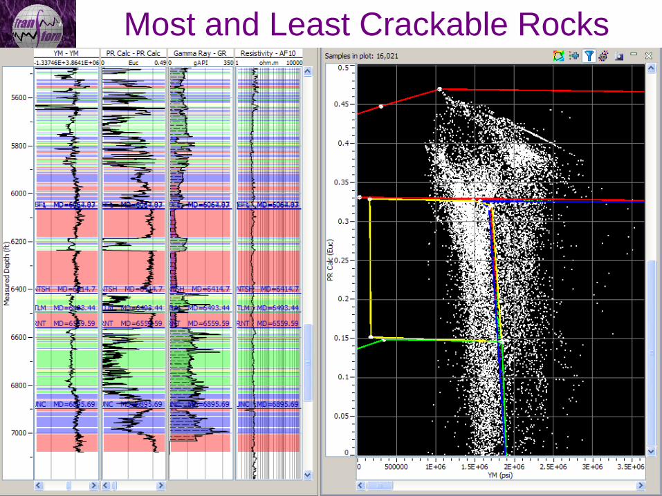
Most and Least Crackable Rocks Young’s Modulus versus Poisson’s Ratio

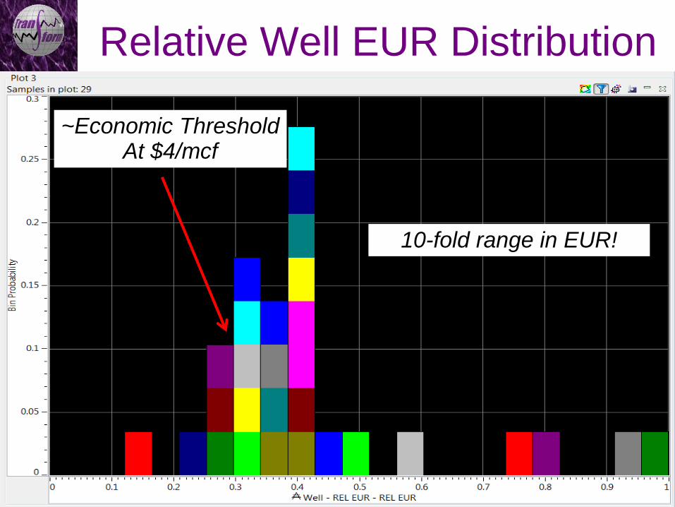
Relative Well EUR Distribution

Transform proprietary information

10-fold range in EUR!

~Economic Threshold At $4/mcf

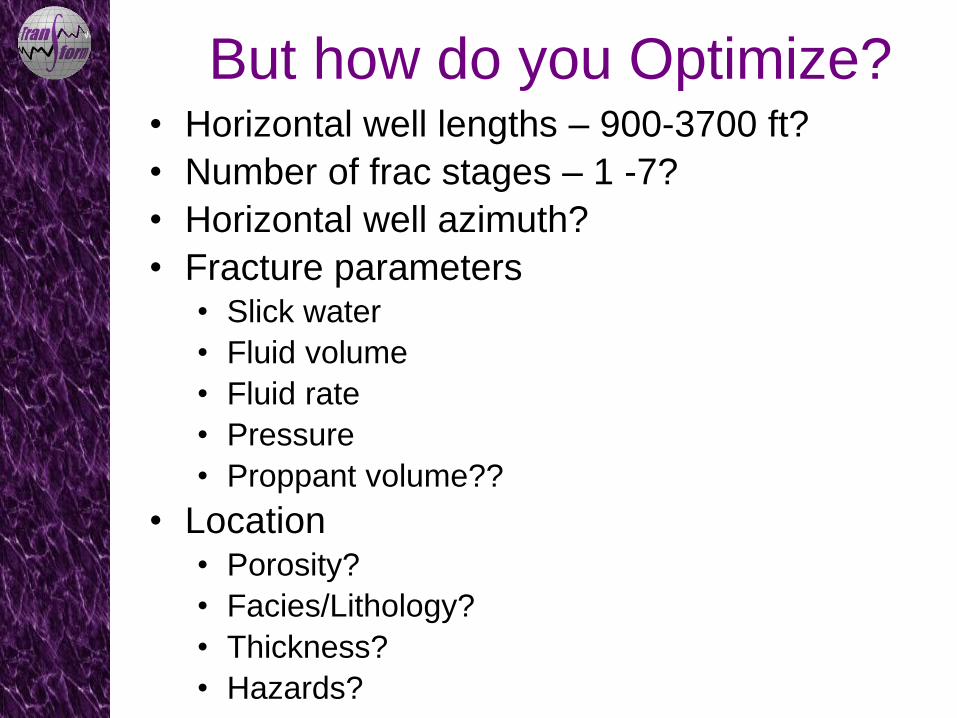
But how do you Optimize? • Horizontal well lengths – 900-3700 ft?

• Number of frac stages – 1 -7?

• Horizontal well azimuth?

• Fracture parameters • Slick water

• Fluid volume

• Fluid rate

• Pressure

• Proppant volume??

• Location • Porosity?

• Facies/Lithology?

• Thickness?

• Hazards?

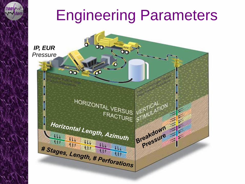
Engineering Parameters

IP, EUR Pressure

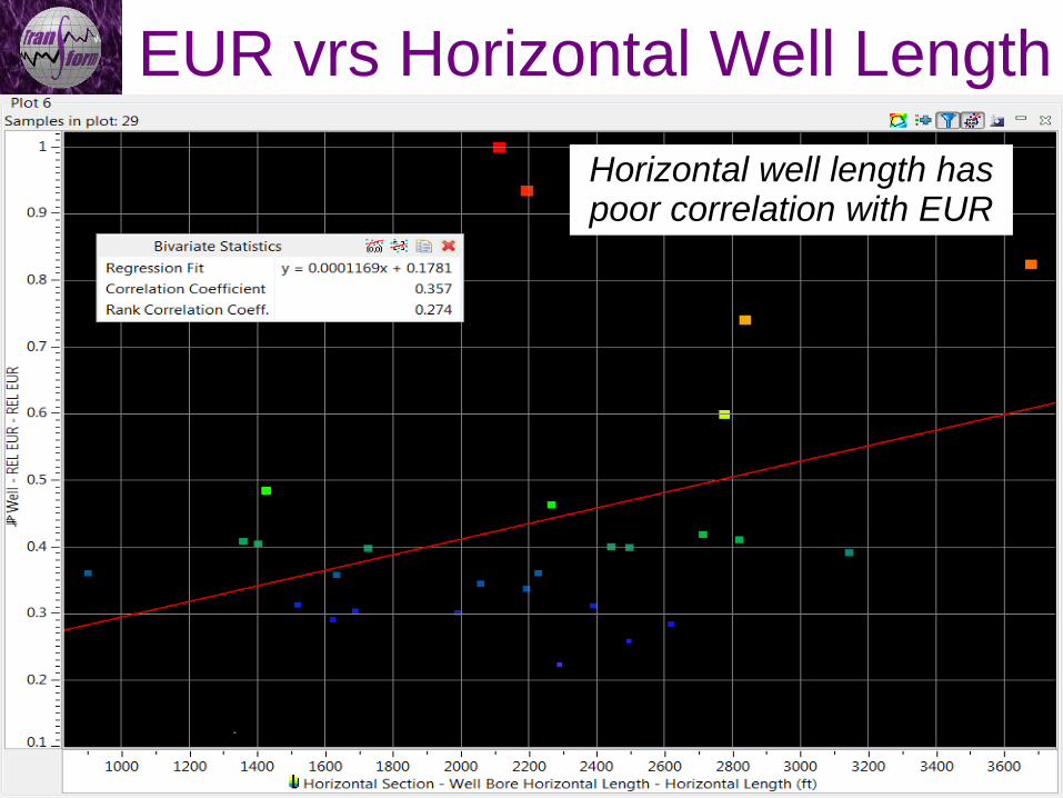
EUR vrs Horizontal Well Length

Transform proprietary information

Horizontal well length has poor correlation with EUR

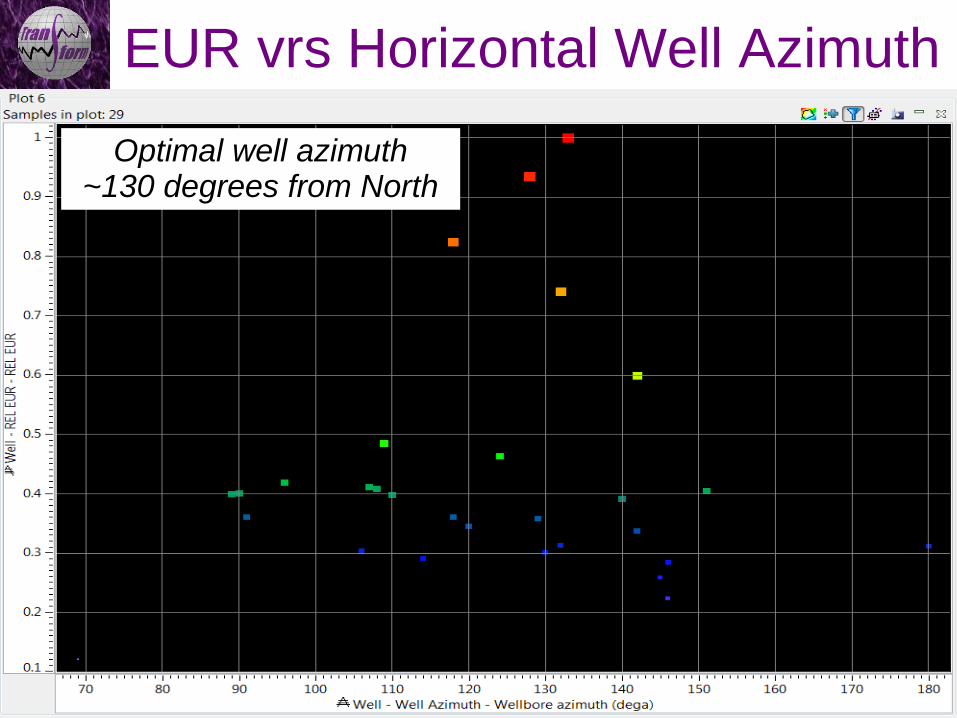
EUR vrs Horizontal Well Azimuth

Transform proprietary information

Optimal well azimuth ~130 degrees from North

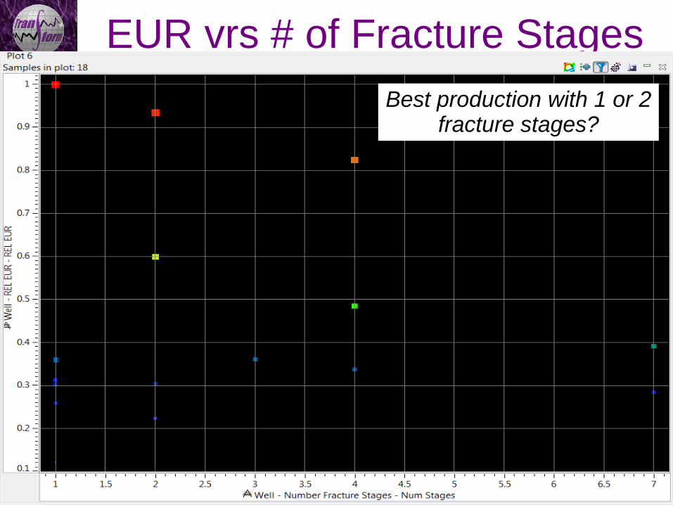
EUR vrs # of Fracture Stages

Transform proprietary information

Best production with 1 or 2 fracture stages?

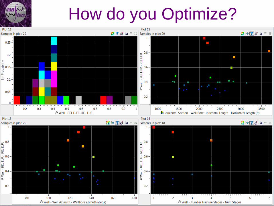
How do you Optimize?

How do you Optimize?

Optimize ->

Shorter Wells?

~130 Degrees? 1 Fracture Stage?

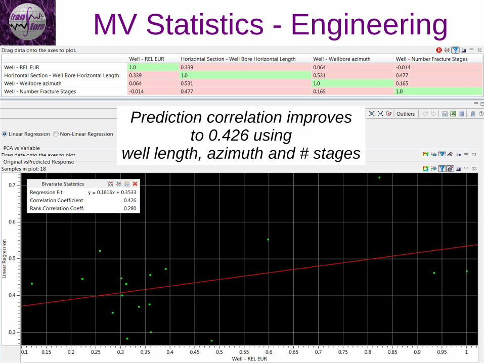
MV Statistics - Engineering

Transform proprietary information

Prediction correlation improves to 0.426 using

well length, azimuth and # stages

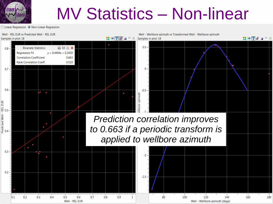
MV Statistics – Non-linear

Prediction correlation improves to 0.663 if a periodic transform is

applied to wellbore azimuth

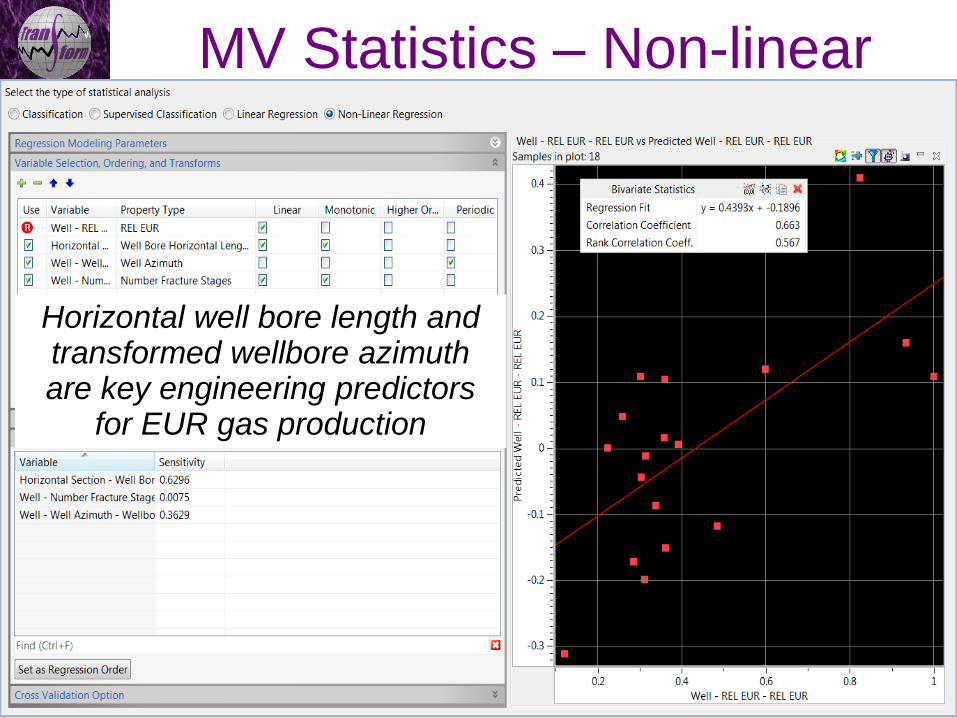
MV Statistics – Non-linear

Horizontal well bore length and transformed wellbore azimuth are key engineering predictors

for EUR gas production

But how do you Optimize? • Horizontal well lengths – 900-3700 ft?

• Number of frac stages – 1 -7?

• Horizontal well azimuth?

• Fracture parameters • Slick water

• Fluid volume

• Fluid rate

• Pressure

• Proppant volume??

• Location • Porosity?

• Facies/Lithology?

• Thickness?

• Hazards?

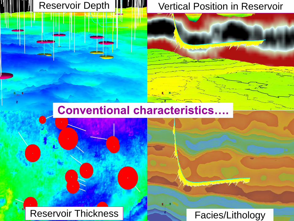
Reservoir Thickness Facies/Lithology

Conventional characteristics….

Reservoir Depth Vertical Position in Reservoir

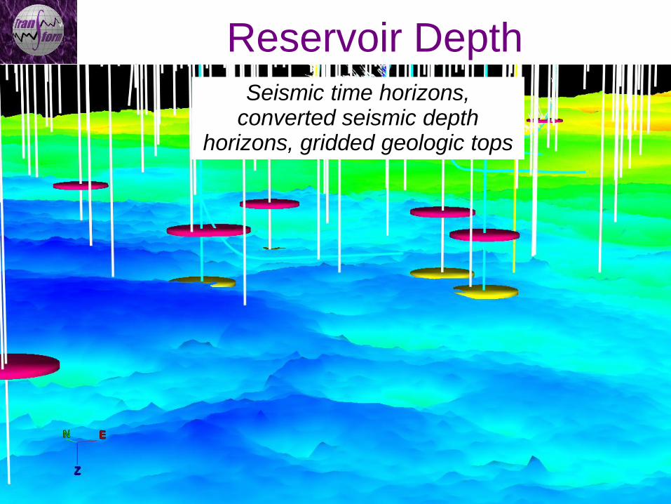
Reservoir Depth

Transform proprietary information

Seismic time horizons, converted seismic depth

horizons, gridded geologic tops

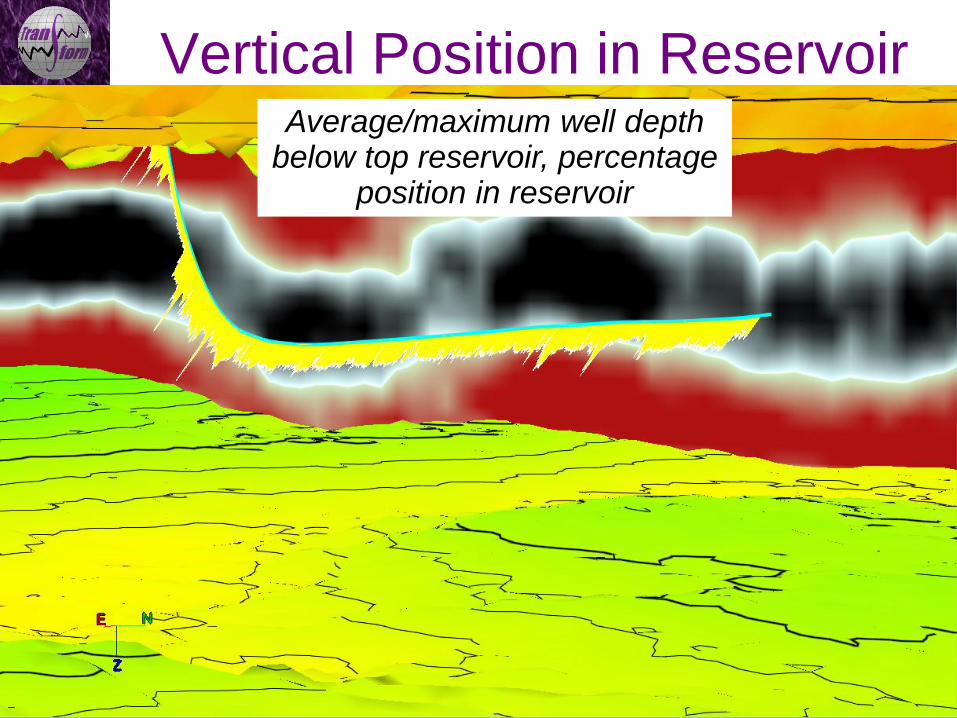
Vertical Position in Reservoir

Transform proprietary information

Distance beneath and between reservoir boundaries

Average/maximum well depth below top reservoir, percentage

position in reservoir

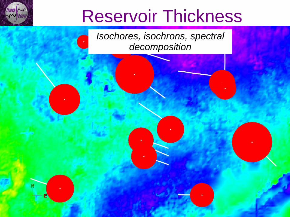
Reservoir Thickness

Transform proprietary information

Distance beneath and between reservoir boundaries

Isochores, isochrons, spectral decomposition

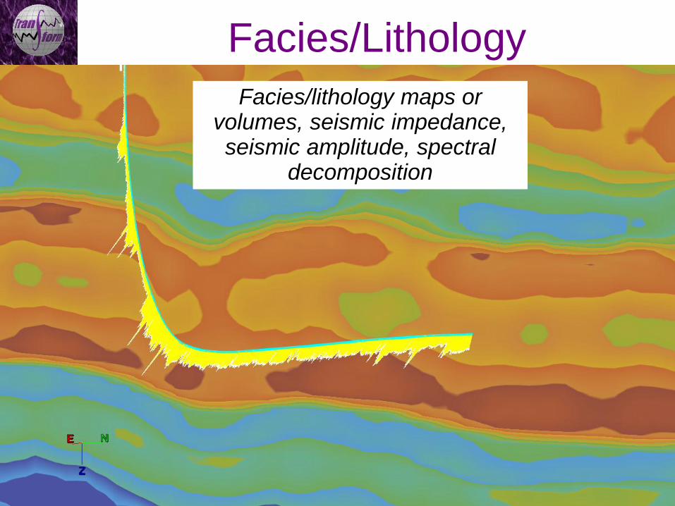
Facies/Lithology

Transform proprietary information

Distance beneath and between reservoir boundaries

Facies/lithology maps or volumes, seismic impedance, seismic amplitude, spectral

decomposition

Reservoir Thickness Facies/Lithology

Conventional characteristics….

Reservoir Depth Vertical Position in Reservoir

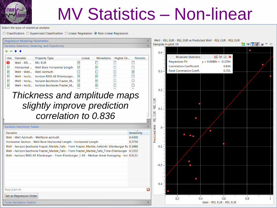
MV Statistics – Non-linear

Thickness and amplitude maps slightly improve prediction

correlation to 0.836

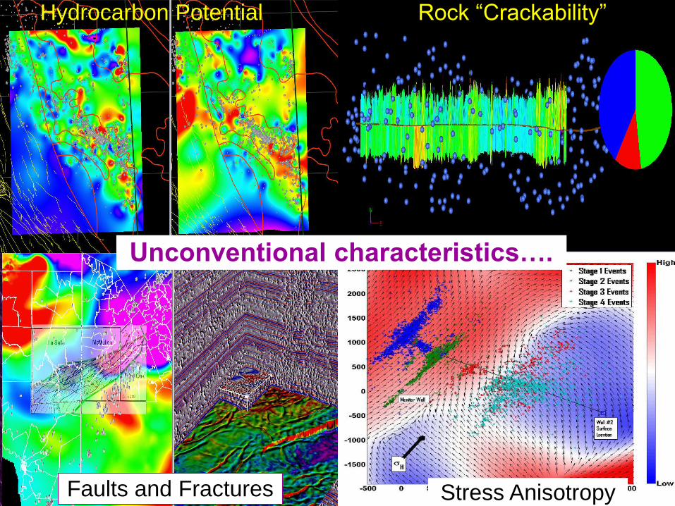
Hydrocarbon Potential Rock “Crackability”

Faults and Fractures Stress Anisotropy

Unconventional characteristics….

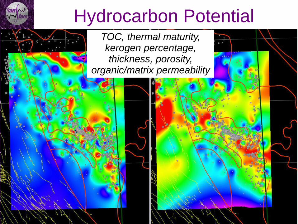
Hydrocarbon Potential

TOC, thermal maturity, kerogen percentage, thickness, porosity,

organic/matrix permeability

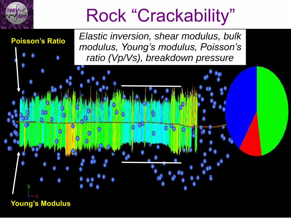
Rock “Crackability”

Elastic inversion, shear modulus, bulk modulus, Young’s modulus, Poisson’s

ratio (Vp/Vs), breakdown pressure

Young’s Modulus

Poisson’s Ratio

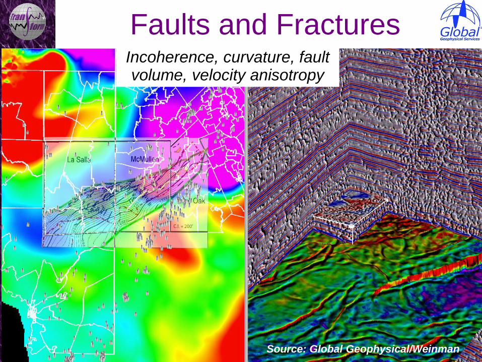
Faults and Fractures Incoherence, curvature, fault volume, velocity anisotropy

Source: Global Geophysical/Weinman

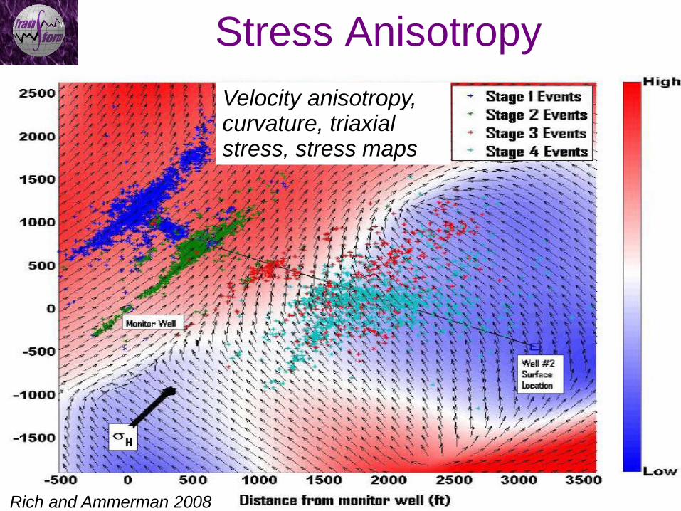
Stress Anisotropy

Velocity anisotropy, curvature, triaxial stress, stress maps

Rich and Ammerman 2008

Hydrocarbon Potential Rock “Crackability”

Faults and Fractures Stress Anisotropy

Unconventional characteristics….

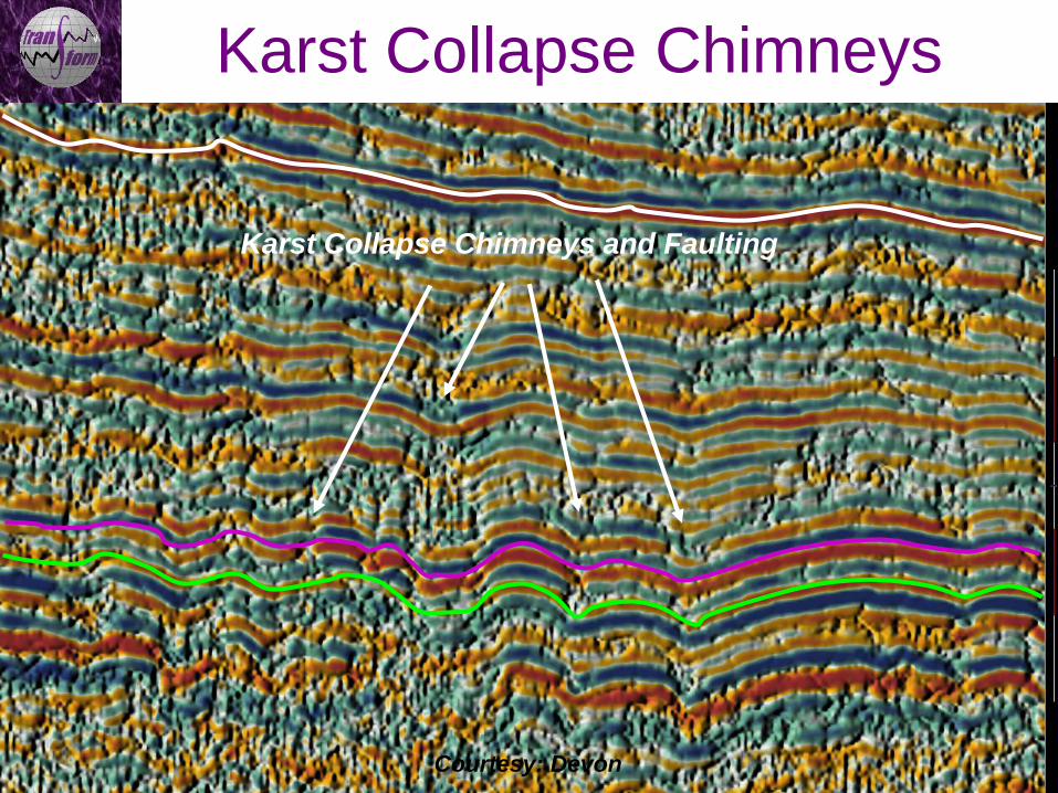
Karst Collapse Chimneys

Karst Collapse Chimneys and Faulting

Courtesy: Devon

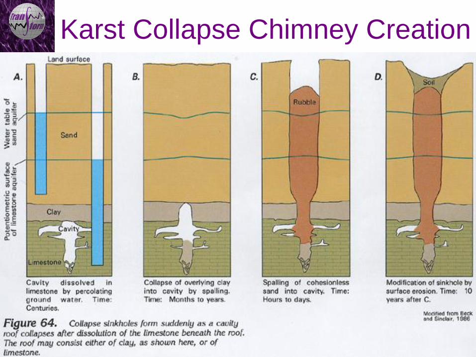
Karst Collapse Chimney Creation

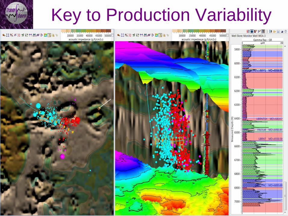
Key to Production Variability

Transform proprietary information

Microseismic Illustrates Paths

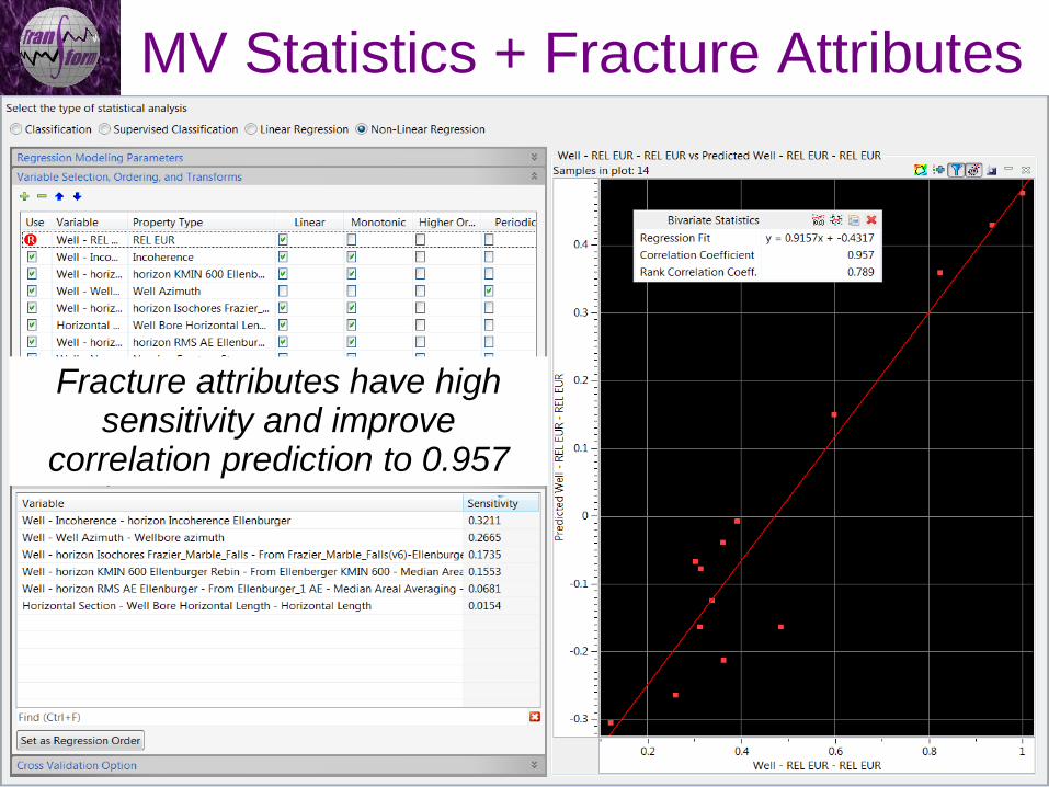
MV Statistics + Fracture Attributes

Transform proprietary information

Fracture attributes have high sensitivity and improve

correlation prediction to 0.957

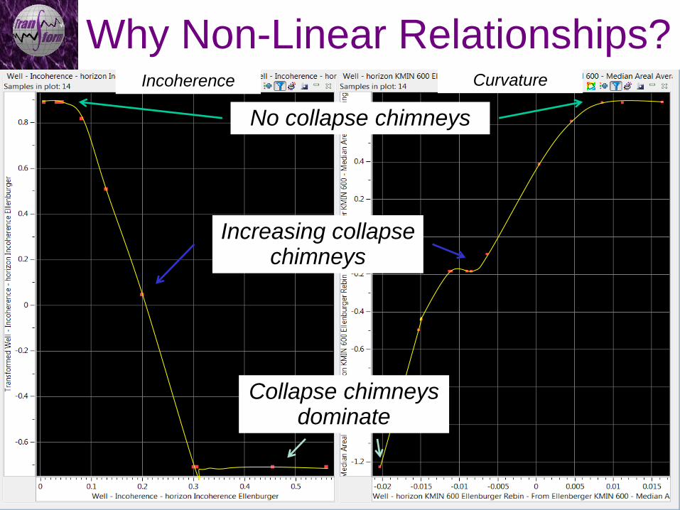
Why Non-Linear Relationships?

No collapse chimneys

Increasing collapse chimneys

Collapse chimneys dominate

Incoherence Curvature

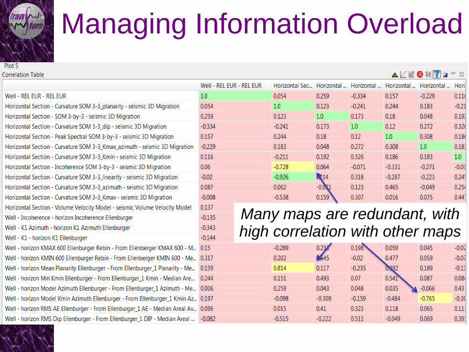
Managing Information Overload

Transform proprietary information

Many maps are redundant, with high correlation with other maps

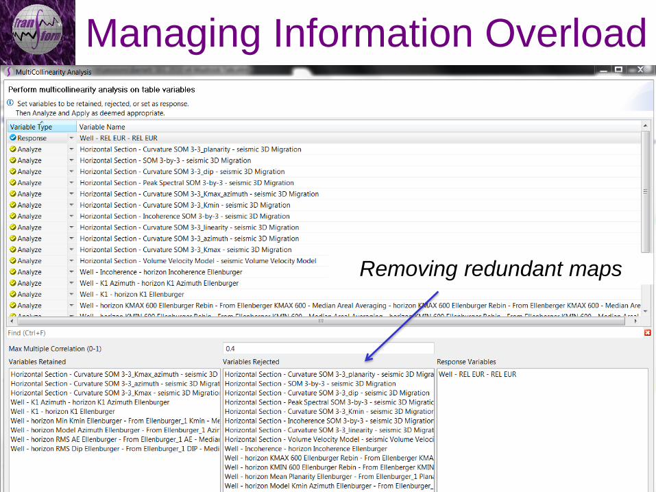
Managing Information Overload

Transform proprietary information

Removing redundant maps

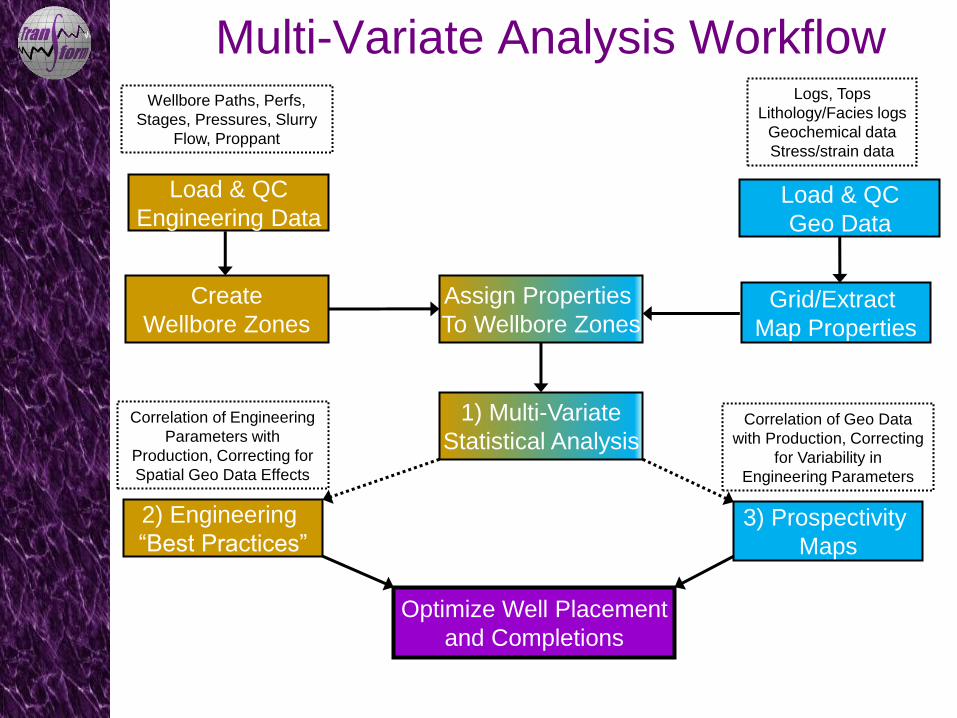
Multi-Variate Analysis Workflow

2) Engineering

“Best Practices”

Optimize Well Placement

and Completions

Assign Properties

To Wellbore Zones

Load & QC

Engineering Data

Wellbore Paths, Perfs,

Stages, Pressures, Slurry

Flow, Proppant

Load & QC

Geo Data

Logs, Tops

Lithology/Facies logs

Geochemical data

Stress/strain data

Grid/Extract

Map Properties

Create

Wellbore Zones

1) Multi-Variate

Statistical Analysis Correlation of Engineering

Parameters with

Production, Correcting for

Spatial Geo Data Effects

3) Prospectivity

Maps

Correlation of Geo Data

with Production, Correcting

for Variability in

Engineering Parameters

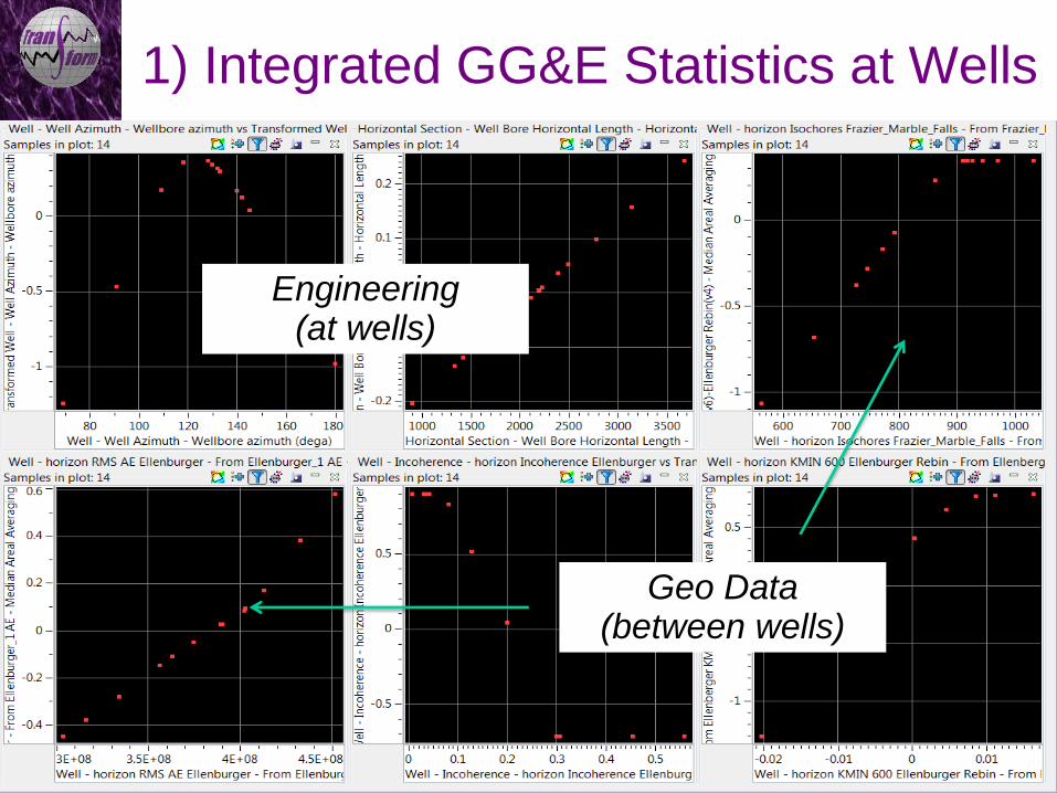
1) Integrated GG&E Statistics at Wells

Transform proprietary information

Engineering (at wells)

Geo Data (between wells)

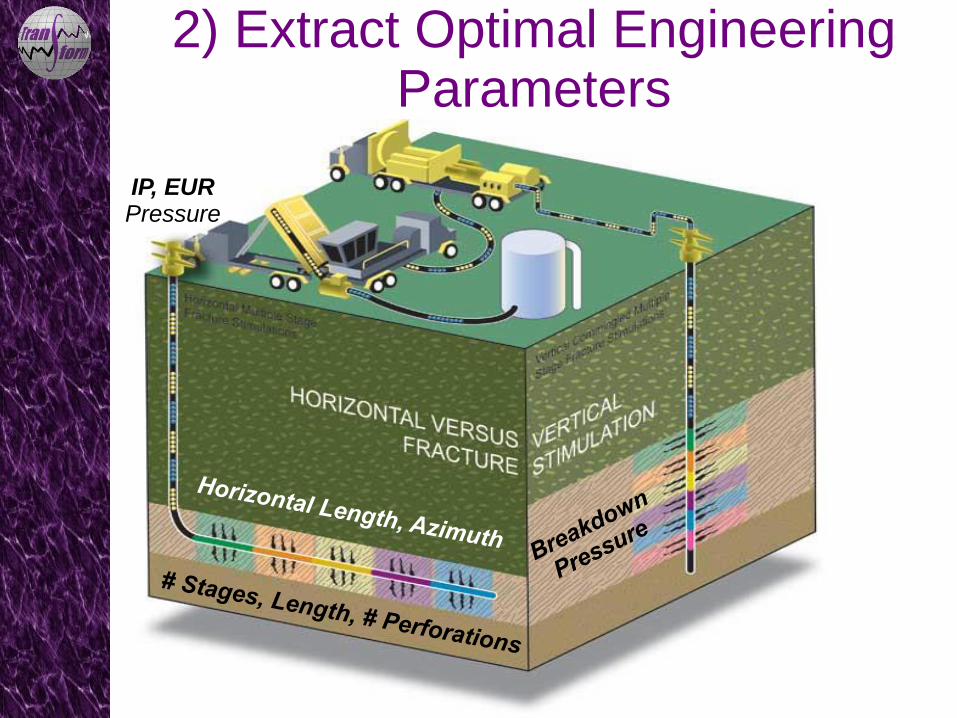
2) Extract Optimal Engineering Parameters

IP, EUR Pressure

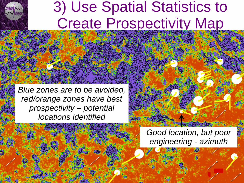
3) Use Spatial Statistics to Create Prospectivity Map

Blue zones are to be avoided, red/orange zones have best

prospectivity – potential locations identified

Good location, but poor engineering - azimuth

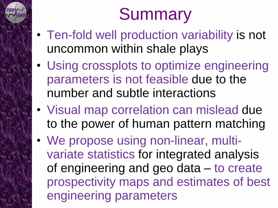
Summary • Ten-fold well production variability is not

uncommon within shale plays

• Using crossplots to optimize engineering parameters is not feasible due to the number and subtle interactions

• Visual map correlation can mislead due to the power of human pattern matching

• We propose using non-linear, multi-variate statistics for integrated analysis of engineering and geo data – to create prospectivity maps and estimates of best engineering parameters

Predicting Shale Production with Integrated Multi-Variate Statistics

Murray Roth

Transform Software and Services, Inc.