Predicting Cumulative Production Predicting Cumulative Production of Devonian Shale Gas Wells from of Devonian Shale Gas Wells from

Early Well Performance Data, Early Well Performance Data, Appalachian Basin of Eastern Appalachian Basin of Eastern

KentuckyKentuckyBrandon C. NuttallBrandon C. Nuttall

Kentucky Geological SurveyKentucky Geological SurveyWith contributions by Shannon DaughertyWith contributions by Shannon Daugherty

Eastern Section AAPG, Lexington, KentuckyEastern Section AAPG, Lexington, Kentucky1717--SepSep--20072007

Funding: National Coal Resources Data System, U. S. Geological Survey

Geology of Devonian ShaleGeology of Devonian Shale

A A ““shaleshale”” well well isis……??

•• Top Sunbury to Top Sunbury to top underlying top underlying carbonatescarbonates

SunburyBerea

Cleveland

Three Lick Bed

Upper Huron

Middle Huron

Lower Huron

Olentangy

Rhinestreet

Ohi

o

Early Performance DataEarly Performance Data

•• Well log and completion reportWell log and completion report–– Initial Open FlowInitial Open Flow–– Rock PressureRock Pressure

•• Monthly production Monthly production (805 KAR 1:180, KRS (805 KAR 1:180, KRS 353.205)353.205)–– Maximum monthly production (Maximum monthly production (McfMcf))–– First year cumulative productionFirst year cumulative production–– 5 year cumulative production5 year cumulative production

Data SetsData Sets

•• KGS online well completion dataKGS online well completion data–– Location, completions, IOF, RPLocation, completions, IOF, RP

•• Division of Oil and GasDivision of Oil and Gas–– Public production data by month (1997)Public production data by month (1997)

•• Gas Technology Institute (GRI)Gas Technology Institute (GRI)–– Historic, longHistoric, long--term production dataterm production data–– ProprietaryProprietary, available to members and , available to members and

contractorscontractors

Production Data SelectionProduction Data Selection

•• Completed since 1Completed since 1--JanJan--9797•• Devonian shale only (not commingled)Devonian shale only (not commingled)•• 60 or more months of non60 or more months of non--zero datazero data•• 310 wells310 wells

Initial Open Flow DataInitial Open Flow Data

•• Exhibits only Exhibits only weak trendsweak trends

•• No uniform No uniform method of method of acquiringacquiring

Reported Reported ““Rock PressureRock Pressure””

•• High and low High and low open flows open flows occur in areas occur in areas of both high of both high and low rock and low rock pressurepressure

Rock Pressure Rock Pressure vsvs IOFIOF

0

500

1000

1500

2000

0 200 400 600 800 1000

Rock Pressure (psi)

IOF

(Mcf

)

FiveFive--year Cumulative Productionyear Cumulative Production

•• Again, weak Again, weak trendstrends

•• Areas with Areas with higher and higher and lower lower production are production are often adjacentoften adjacent

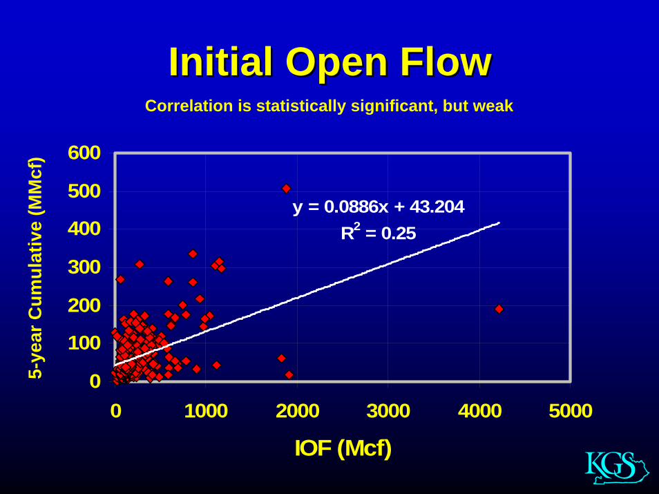
Initial Open FlowInitial Open Flow

y = 0.0886x + 43.204R2 = 0.25

0

100

200

300

400

500

600

0 1000 2000 3000 4000 5000

IOF (Mcf)

5-ye

ar C

umul

ativ

e (M

Mcf

)

Correlation is statistically significant, but weak

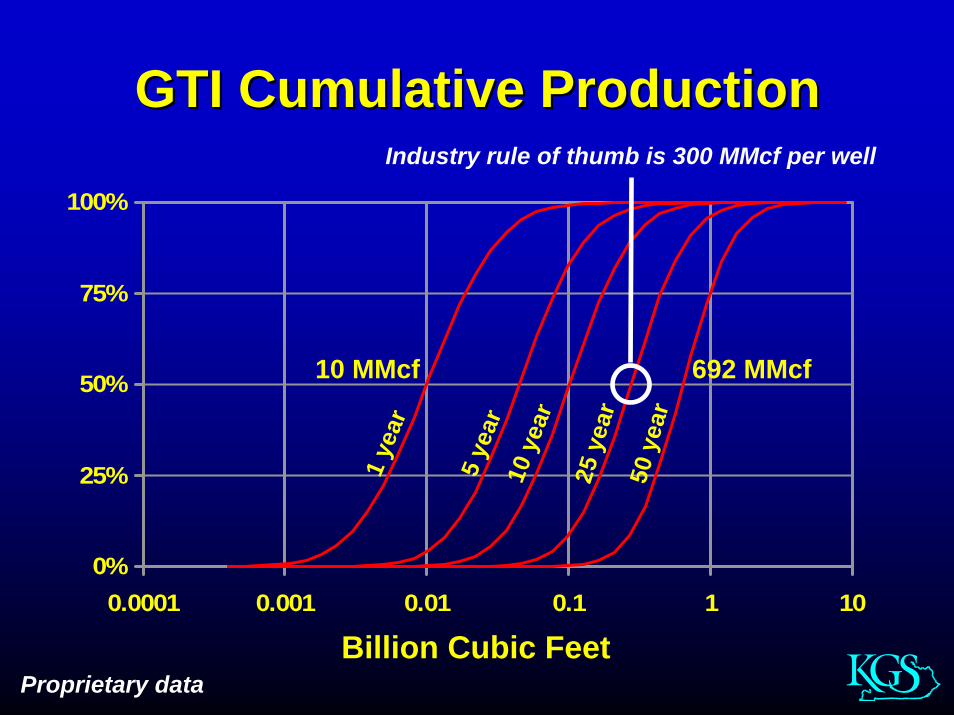
GTI Cumulative ProductionGTI Cumulative Production

0%

25%

50%

75%

100%

0.0001 0.001 0.01 0.1 1 10

1 ye

ar

5 ye

ar10

yea

r25

yea

r50

yea

rBillion Cubic Feet

10 MMcf 692 MMcf

Proprietary data

Industry rule of thumb is 300 MMcf per well

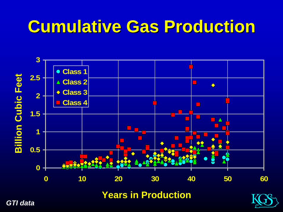
Cumulative Gas ProductionCumulative Gas Production

0

0.5

1

1.5

2

2.5

3

0 10 20 30 40 50 60

Class 1Class 2Class 3Class 4

Years in Production

Bill

ion

Cub

ic F

eet

GTI data

Cumulative Production Over Cumulative Production Over TimeTime

y = 1.8887x + 7.0426R2 = 0.9278

0

200

400

600

800

1000

1200

0 100 200 300 400 500 600

Five-year (MMcf)

Ten-

year

(MM

cf)

GTI data

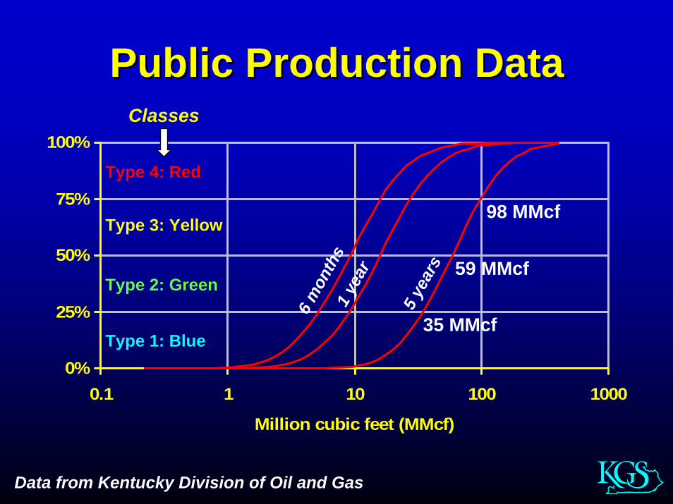
Public Production Data Public Production Data

0%

25%

50%

75%

100%

0.1 1 10 100 1000

Million cubic feet (MMcf)

35 MMcf

59 MMcf

98 MMcf

Type 1: Blue

Type 2: Green

Type 3: Yellow

Type 4: Red

Classes

Data from Kentucky Division of Oil and Gas

6 m

onth

s1

year

5 ye

ars

General Decline Model (General Decline Model (ArpsArps))

( )bi

it

tbD

qq 11+

=Hyperbolic:

Best fit parameters:qi – initial productionDi – nominal declineb – decline exponent

Special cases:

tDi

t ieqq =Exponential, b=0: Harmonic, b=1: ( )tD

qqi

it +=

1

SolvingSolvingExponential:

( ) ( ) tDqq iit += lnlnLeast squares

Hyperbolic:OptimizationLinear Programming

Both can easily be done with the built-in functions supplied with spreadsheets, but…

Best Case: Best Case: Textbook DataTextbook Data

Deplete free gas in fractures

Desorbs from fracture faces Desorption and

diffusion through shale matrix

Natural fracturing is key to production

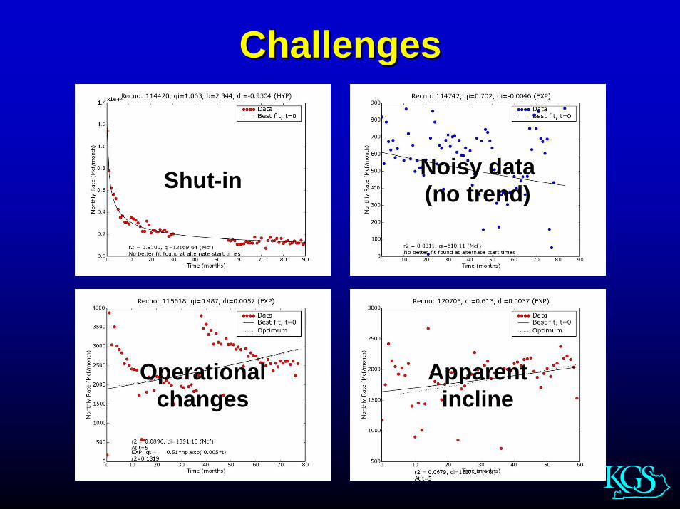
ChallengesChallenges

Noisy data(no trend)

Apparentincline

Shut-in

Operationalchanges

Raw DataRaw Data

NormalizedNormalized

maxqqq obs

t =

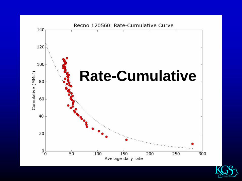
RateRate--CumulativeCumulative

Semi-log plot

Rule of thumb:b ≈ 3 to 4

Rule of thumb:Di ≈ -0.95 to -0.99

Many data sets have a “decline” (i.e., slope) that is not statistically different from 0 (no correlation).

Max production is the initial period

For exponential decline, Qi is often less than max production

For hyperbolic decline, Qi is often greater than max production

Qi and maximum production are not correlated

Basis of classification

25th percentile50th percentile

75th percentile

Public data from the Kentucky Division of Oil and Gas

6moCum = 101.7*MaxAvg + 1938r2 = 0.87

Public data from the Kentucky Division of Oil and Gas

Type DeclinesType Declines

0

50

100

150

200

0 12 24 36 48 60

Months

Type 1: 143MMcf Type 2: 78 MMcf Type 3: 46 MMcfType 4: 23 MMcf

Ave

rage

Mcf

/d

Five-year cumulative production in million cubic feet

ConclusionsConclusions•• Shale production data is messyShale production data is messy•• Decline curve analysis and reserves Decline curve analysis and reserves

projection is an artprojection is an art•• Maximum average daily production during Maximum average daily production during

the first 6 months is an adequate indicator of the first 6 months is an adequate indicator of future well performancefuture well performance

•• Best wells can be expected to make:Best wells can be expected to make:–– 20 20 MMcfMMcf in first yearin first year–– 100 100 MMcfMMcf after 5 yearsafter 5 years

ThanksThanks

•• www.uky.edu/kgswww.uky.edu/kgs•• bnuttall@uky.edubnuttall@uky.edu•• Oil and gas well search with production Oil and gas well search with production

datadata–– kgsweb.uky.edu/DataSearching/OilGas/OGSearch.aspkgsweb.uky.edu/DataSearching/OilGas/OGSearch.asp

•• Oil and gas well interactive mappingOil and gas well interactive mapping–– kgsmap.uky.edu/website/KGSGeology/viewer.aspkgsmap.uky.edu/website/KGSGeology/viewer.asp

•• Project web pageProject web page–– www.uky.edu/KGS/emsweb/devsh/production/index.htmwww.uky.edu/KGS/emsweb/devsh/production/index.htm