Practical model calibrationMichael Boguslavsky,

ABN-AMRO Global Equity Derivatives

Presented at RISK workshop, New York, September 20-21, 2004

What is this talk about Pitfalls in fitting volatility surfaces Hints and tips

Disclaimer: The models and trading opinions presented do not represent models and trading

opinions of ABN-AMRO

Overview

1: estimation vs fitting

2: fitting: robustness and choice of metric

3: no-arbitrage and no-nonsense

4: estimation techniques

5: solving data quality issues

6: using models for trading

1. Estimation vs fitting In different situations one needs different models or

smile representations

marketmaking

exotic pricing

risk management

book marking

Two sources of data for the model

real-world underlying past price series

current derivatives prices and fundamental information

1.1 Smile modelling approaches

“single maturity models”

estimation fitting

Join estimation & fitting

parameterisationsmodels

1.1 Smile modelling approaches (cont)

•Models:–Bachelier & Black-Scholes

–Deterministic volatility and local volatility

–Stochastic Volatility

–Jump-diffusions

–Levy processes and stochastic time changes

–Uncertain volatility and Markov chain switching volatility

–Combinations:–Stochastic Volatility+Jumps

–Local volatility+Stochastic volatility

–...

1.1 Smile modelling approaches (cont)

Some models do not fit the market very well, less parsimonious ones fit

better (does not mean they are better!)

Multifactor models can not be estimated from underlying asset series alone

(one needs either to assume something about the preference structure or to

use option prices)

Some houses are using different model parameters for different maturities -

a hybrid between models and smile parameterisations

Heston with parameters depending smoothly on time

SABR in some forms

1.1 Smile modelling approaches (cont)

Parameterisations:

In some cases, one is not interested in the model for stock price movement, but just in a

“joining the dots” exercise

Example: a listed option marketmaker may be more interested in fit versatility than in

consistency and exotic hedges

Typical parameterisations:

splines

two parabolas in strike or log-strike

kernel smoothing

etc

Many fitting techniques are quite similar for models and parameterisations

1.1 Smile modelling approaches (cont)

A nice parameterisation:

cubic spline for each maturity

fitting on tick data

penalties for deviations from last quotes (time decaying weights)

penalties for approaching too close to bid and ask quotes, strong penalties for breaching them

penalty for curvature and for coefficient deviation from close maturities

1.1 Example: low curvature spline fit to bid/offer/last

Hang Seng Index options

7 nodes

linear extrapolation

intraday fit

1.2 Models: estimation and fitting Will they give the same result? A tricky question, as one needs

a lot of historic data to estimate reliably

stationarity assumption to compare forward-looking data with past-looking

assumptions on risk preferences

1.2 Estimation vs fitting: example, Heston model

withtttt

tttttt

dZvdtvdv

dBSvdtSdS

)(

dZdb,(Girsanov) measures neutralrisk and physicalunder same theare and

1.2 Estimation vs fitting: example, Heston model (cont)

However, very often estimated are very far from option implied

some studies have shown that in practice skewness and kurtosis are much higher in

option markets

Bates

Bakshi, Cao, Chen

Possible causes:

model misspecification e.g. extra risk factors

peso problem

insufficient data for estimation (>Javaheri)

trade opportunity?

and

1.3: Similar problems Problem of fitting/estimating smile is similar to

fitting/estimating (implied) risk-neutral density (via

Breeden&Litzenberger’s formula)

But smile is two integrations more robust

),()exp(),(2

2

XfrTX

KTC

2: fitting: robustness and choice of metric

2.1 What do we fit to?

There is no such thing as “market prices”

We can observe

last (actual trade prices)

end-of-day mark

bid

ask

2.1 What do we fit to? Last prices:

much more sparse than bid/ask quotes

not synchronized in time End-of day marks

available once a day

indications, not real prices Bid/ask quotes

much higher frequency than trade data

synchronized in time

tradable immediately Often people use mid price or mid volatility quotes

discarding extra information content of separate bid and ask quotes

2.2 Standard approaches Get somewhere “market” price for calls and puts (mid or

cleaned last) Compose penalty function

least squares fit in price (calls, puts, blend)

least squares fit in vol

other point-wise metrics e.g. mean absolute error in price or vol

Minimize it using one’s favourite optimizer

2.2 Standard approaches (cont) Formally:

min))(()(

functionpenalty or 1,2,usually used;exponent metric -

weights-urity strike/mat and parametersfor measure price model- )(

parameters model ofvector -ies volatilitimpliedor options

OTM of pricescash e.g. prices,market of measures - maturity and strikegiven h option witfor number index -

i

iii

i

i

i

PwM

wi

Pi

2.2 Standard approaches (cont) Problem: why do we care about the least-squares?

May be meaningful for interpolation

useless for extrapolation

useless for “global” or second order effects

always creates unstable optimisation problem with multiple local minima

2.2 Standard approaches (cont) Some people suggest using global optimizers to solve

the multiple local minima problem

simulated annealing

genetic algorithms

They are slow And, actually, they do not solve the problem:

2.2 Standard approaches (cont) Suppose we have a perfect

(and fast!) global optimizer

true local minima may change discontinuously with market prices!

=> Large changes in process parameters on recalibration

2.3 Which metric to use? Ideally, we would want to have a low-dimensional linear optimization

problem

all process parameters are tradable/observable - not realistic

It is Ok if the problem is reasonably linear

Luckily, in many markets we observe vanilla combination prices

FX: risk reversal and butterfly prices are available

equity: OTC quoted call and put spreads

=>smile ATM skew and curvature are almost directly observable!

2.3 Which metric to use? (cont) Many models have reasonably linear dependence between process

parameters and smile level/skew/curvature around the optimum

Actually, these are the models traders like most, because they think in terms of smile level/skew/curvature and can (kind of) trade them

Thus, one can e.g. minimize a weighted sum of vol level, skew, and curvature squared deviations from option/option combination quotes

Example: Heston model fit on level/skew/curvature

•DAX Index options,

•Heston model

• global fit

2.4 Additional inputs Sometimes, it is possible to use additional inputs in

calibration

variance swap price: dictates the downside skew (warning: dependent on the cut-off level!)

Equity Default Swap price: far downside skew (warning: very model-dependent!)

view on skew dynamics from cliquet prices

2.5 Fitting: a word of caution Even if your model perfectly fits vanilla option prices, it does not

mean that it will give reasonable prices for exotics!

Schoutens, Simons, Tistaert:

fit Heston, Heston with exponential jump process, variance Gamma, CGMY, and several other stochastic volatility models to Eurostoxx50 option market

all models fit pretty well

compare then barrier, one-touch, lookback, and cliquet option prices

report huge discrepancies between prices

2.5 Fitting: a word of caution (cont)

Examples:

smile flattening in local volatility models

Local Volatility Mixture of Densities/Uncertain volatility model of Brigo, Mercurio, Rapisarda (Risk, May 2004):

at time 0+ volatility starts following of of the few prescribed trajectories with probability

thus, the marginal density of S at time t is a linear combination of marginal densities of several different local volatility models (actually, the authors use ), so the density is a mixture of lognormals

ttttt dwSStdtStytrdS ),())()((

),( tSii

),(not ),( tii Stt

2.5 Fitting: a word of caution (cont)

Perfect fitting of the whole surface of Eurostoxx50 volatility with just 2-3 terms

Zero prices for variance butterflies that fall between volatility scenarios

Actually (almost) the same happens in Heston model

Scenario 1, p=0.54

Scenario 2, p=0.46

Vol butterfly

vol

T

3: no-arbitrage and no-nonsense Mostly important for parameterisations, not for models This is one of the advantages of models However, some checks are useful, especially in the tails

s)butterflie ratio negative-(non

,0)()()()(

prices) (monotonic 0)()(

prices) negative-(non 0)(

2312

321

21

KKb

KKa

KCabKbCKaC

KCKC

KC

3.1 No arbitrage: single maturity Fixed maturity European call prices:

3.1 No arbitrage: single maturity (cont)

Breeden&Litzenberger’s formula:

where f(X) is the risk-neutral PDF of underlying at time T

Our three conditions are equivalent to

Non-negative integral of CDF

Non-negative CDF

Non-negative PDF

),()exp(),(2

2

XfrTX

KTC

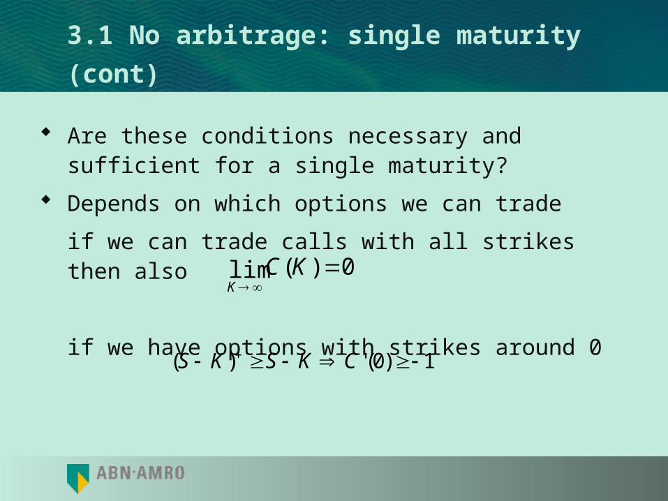
3.1 No arbitrage: single maturity (cont) Are these conditions necessary and sufficient for a single

maturity? Depends on which options we can trade

if we can trade calls with all strikes then also

if we have options with strikes around 0

0)(lim

KCK

1)0(')( CKSKS

3.1 No arbitrage: single maturity (cont)

Example

No dividends, zero interest rate

C(80)=30, C(90)=21, C(100)=14

is there an arbitrage here?

3.1 No arbitrage: single maturity (cont)

All spreads are positive, 80-90-100 butterfly is worth 30-2*21+14=2>0...

But Payoff diagram:

041)90()80(

89

81

CCS

0 80 90

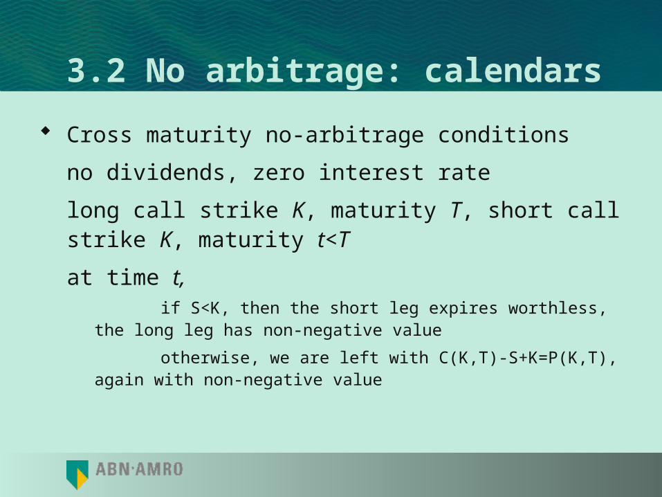
3.2 No arbitrage: calendars Cross maturity no-arbitrage conditions

no dividends, zero interest rate

long call strike K, maturity T, short call strike K, maturity t<T

at time t,if S<K, then the short leg expires worthless, the long leg has

non-negative value

otherwise, we are left with C(K,T)-S+K=P(K,T), again with non-negative value

3.2 No arbitrage: calendars Thus, with no dividends, zero interest rate,

This is model independent With dividends and non-zero interest rate, one has to

adjust call strike for the carry on stock and cash positions

),(),( tKCTKC

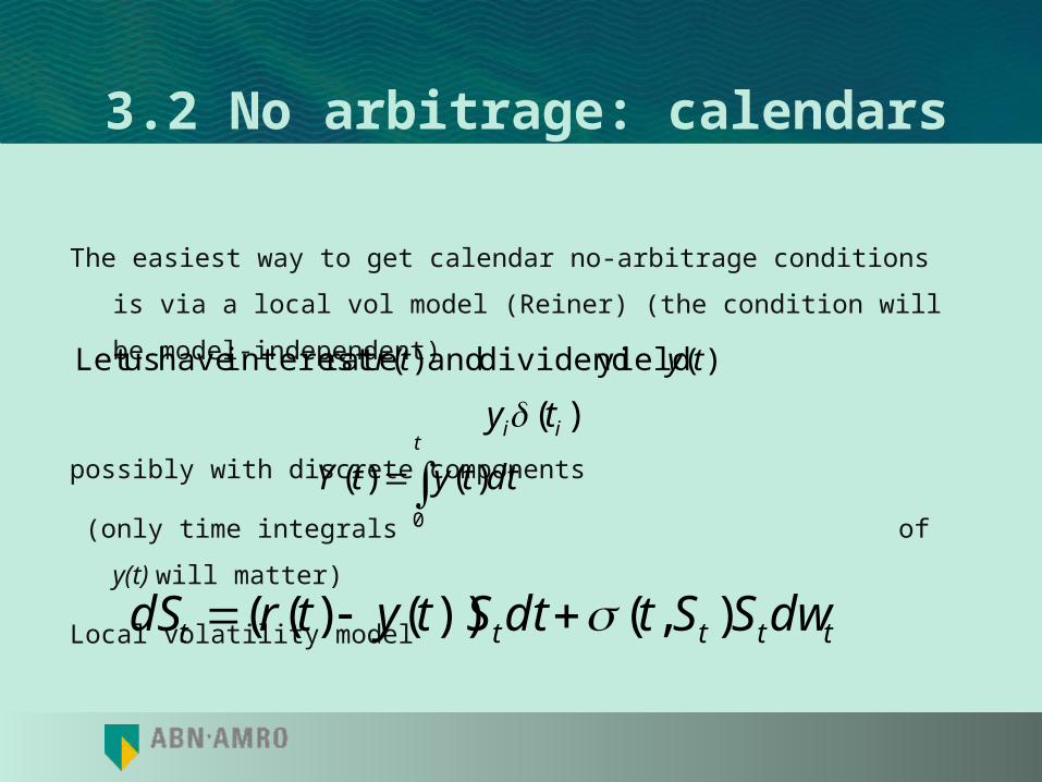
3.2 No arbitrage: calendars

The easiest way to get calendar no-arbitrage conditions is via a local vol

model (Reiner) (the condition will be model-independent)

possibly with discrete components

(only time integrals of y(t) will matter)

Local volatility model

)( yield dividend and )( rateinterest have usLet tytr

)( ii ty

ttttt dwSStdtStytrdS ),())()((

t

dttytY0

)()(

3.2 No arbitrage: calendars (cont) Consider a portfolio consisting of

long position in an option with strike K and maturity T

short position in

TT

tRTRtYTY

tYTY

dttrTRdttyTY

Kek

te

00

))()(()()(

)()(

,)()( ,)()(

,

strike and maturity with call of units

3.2 No arbitrage: calendars (cont) As before, at time t,

if S<K, then the short leg expires worthless, the long leg has non-negative value

otherwise, we are left with

has non-negative value

),()(),( )()( TKPKSeTKC TYtY

3.3 No nonsense Unimodal implied risk-neutral density

can be interpolation-dependent if one is not careful! reasonable implied forward variance swap prices

again, make sure to use good interpolation

3.3 No nonsense (cont)

Model-specific constraints

Example: Heston+Merton model

correlation should be negative (equities)

mean reversion level should be not too far from the volatility of longest

dated option at hand

volatility goes to infinity for strike iff CDS price is positive

, otherwise volatility can go 0 and stay around it (not a

feasible constraint)

02

21

4: estimation techniques

Most advances are for affine jump-diffusion models

First one: Gaussian QMLE (Ruiz; Harvey, Ruiz, Shephard)

does not work very well because of highly non-Gaussian data

Generalized, Simulated, Efficient Methods of Moments

Duffie, Pan, and Singleton; Chernov, Gallant, Ghysels, and Tauchen

(optimal choice of moment conditions), …

Filtering

Harvey (Kalman filter), Javaheri (Extended KF, Unscented KF), ...

Bayesian (Markov chain Monte Carlo) (Kim, Shephard, and Chib), ...

4: Estimation techniques (cont)

Can not estimate the model form underlying data alone without additional

assumptions

Econometric criteria vs financial criteria: in-sample likelihood vs out-of-

sample price prediction

Different studies lead to different conclusions on volatility risk premia,

stationarity of volatility, etc

Much to be done here

5: solving data quality issues

Data are sparse,

non-synchronised,

noisy,

limited in range

Not everything is observeddividends and borrowing rates need to be estimated

Not all prices reported are propersome exchanges report combinations traded as separate trades

5: solving data quality issues (cont)

If one has concurrent put and call prices, one can back-out implied forward

Using high-frequency data when possible

Using bid and ask quotes instead of trade prices (usually there are about 10-50 times more bid/ask quote revisions than trades)

6:using models for trading What to do once the model is fit?

We can either make the market around our model price and hope our position will be reasonably balanced

Or we can put a lot of trust into our model and take a view based on it

6: using models for trading (cont)

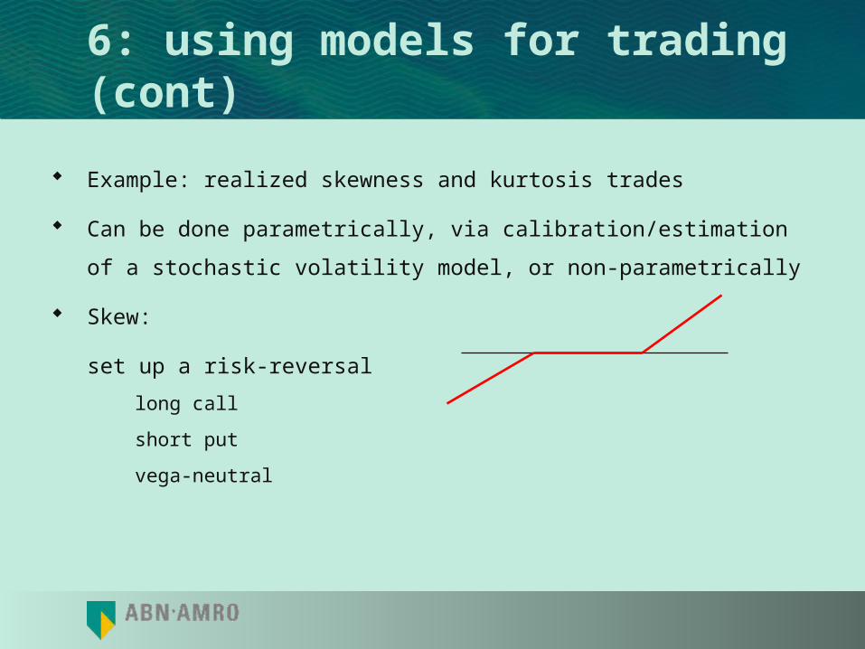
Example: realized skewness and kurtosis trades

Can be done parametrically, via calibration/estimation of a stochastic

volatility model, or non-parametrically

Skew:

set up a risk-reversal

long call

short put

vega-neutral

6: using models for trading (cont) Kurtosis trade:

long an ATM butterfly

short the wings

Actually a vega-hedged short variance swap or some path-dependent exotics would do better

6: using models for trading (cont) Problems:

what is a vega hedge - model dependent

skew trade: huge dividend exposure on the forward

kurtosis trade: execution

peso problem

when to open/close position?

6: using models for trading A simple example: historical vs implied distribution

moments Blaskowitz, Hardle, Schmidt: Compare option-implied distribution parameters with

realized DAX index Assuming local volatility model

Historical vs implied distribution: StDev

Image reproduced with authors’ permission from Blaskowitz, Hardle, Schmidt

Historical vs implied distribution: skewness

Image reproduced with authors’ permission from Blaskowitz, Hardle, Schmidt

Historical vs implied distribution: kurtosis

Image reproduced with authors’ permission from Blaskowitz, Hardle, Schmidt

References

At-Sahalia Yacine, Wang Y., Yared F. (2001) “Do Option Markets Correctly Price the Probabilities of Movement of the UnderlyingAsset?”

Journal of Econometrics, 101

Alizadeh Sassan, Brandt M.W., Diebold F.X. (2002) “Range- Based Estimation of Stochastic Volatility Models” Journal of Finance, Vol. 57,

No. 3

Avellaneda Marco, Friedman, C., Holmes, R., and Sampieri, D., ``Calibrating Volatility Surfaces via Relative-Entropy Minimization’’, in Collected Papers of

the New York University Mathematical Finance Seminar, (1999)

Bakshi Gurdip, Cao C., Chen Z. (1997) “Empirical Performance of Alternative Option Pricing Models” Journal of Finance,Vol. 52, Issue 5

Bates David S. (2000) “Post-87 Crash Fears in the S&P500 Futures Option Market” Journal of Econometrics, 94

Blaskowitz Oliver J., Härdle W., Schmidt P ``Skewness and Kurtosis Trades’’, Humboldt University preprint, 2004.

Bondarenko, Oleg, ``Recovering risk-neutral densities: a new nonparametric approach”, UIC preprint, (2000).

References (cont)Brigo, Damiano, Mercurio, F., Rapisarda, F., ``Smile at Uncertainty,’’ Risk, (2004), May issue.

Chernov, Mikhail, Gallant A.R., Ghysels, E., Tauchen, G "Alternative Models for Stock Price Dynamics," Journal of Econometrics , 2003

Coleman, T. F., Li, Y., and Verma, A ``Reconstructing the unknown local volatility function,’’ The Journal of Computational Finance, Vol. 2, Number 3, (1999), 77-102,

Duffie, Darrell, Pan J., Singleton, K., ``Transform Analysis and Asset Pricing for Affine Jump-Diffusions,’’ Econometrica 68, (2000), 1343-1376.

Harvey Andrew C., Ruiz E., Shephard Neil (1994) “Multivariate Stochastic Variance Models” Review of Economic Studies,Volume 61, Issue 2

Jacquier Eric, Polson N.G., Rossi P.E. (1994) “Bayesian Analysis

of Stochastic Volatility Models” Journal of Business and Economic Statistics, Vol. 12, No, 4

Javaheri Alireza, Lautier D., Galli A. (2003) “Filtering in Finance” WILMOTT, Issue 5

References (cont)

Kim Sangjoon, Shephard N., Chib S. (1998) “Stochastic Volatility: Likelihood Inference and Comparison with ARCH

Models” Review of Economic Studies, Volume 65

Rookley, C., ``Fully exploiting the information content of intra day option quotes: applications in option pricing and risk management,’’ University

of Arizona working paper, November 1997.

Riedel, K., ``Piecewise Convex Function Estimation: Pilot Estimators’’, in Collected Papers of the New York University Mathematical Finance

Seminar, (1999)

Schonbucher, P., “A market model for stochastic implied volatility”, University of Bonn discussion paper, June 1998.