polymer flow in package sealing process - … flow in package ... 6 fluid structure interaction...

Master’s DissertationStructural

Mechanics

HENRIK JOHANSSON and JONATHAN OLLAR

POLYMER FLOW IN PACKAGESEALING PROCESS - A Coupled Eulerian-Lagrangian Numerical Approach

Denna sida skall vara tom!

Copyright © 2011 by Structural Mechanics, LTH, Sweden.Printed by Wallin & Dalholm Digital AB, Lund, Sweden, May, 2011 (Pl).

For information, address:

Division of Structural Mechanics, LTH, Lund University, Box 118, SE-221 00 Lund, Sweden.Homepage: http://www.byggmek.lth.se

Structural MechanicsDepartment of Construction Sciences

Master’s Dissertation by

HENRIK JOHANSSON and JONATHAN OLLAR

Supervisors

Kent Persson, PhD,Div. of Structural Mechanics

ISRN LUTVDG/TVSM--11/5175--SE (1-72)ISSN 0281-6679

POLYMER FLOW IN PACKAGE

SEALING PROCESS

- A Coupled Eulerian-Lagrangian

Numerical Approach

Examiner:

Per-Erik Austrell, Assoc. Professor,Div. of Structural Mechanics

Eskil Andreasson, MSc,Tetra Pak

ABSTRACT

Tetra Pak produces packages designed to contain liquid products. This report is focusedon the sealing process of the packages. These are made through compressing and heatingof laminated paper through which the plastic laminates melt and merge.

The long term goal for Tetra Pak is to be able to predict the outcome of different setupsin the sealing process by the use of virtual models. In this thesis the Coupled Eulerian-Lagrangian formulation in Abaqus 6.10 has been evaluated as a tool for this.

In the journey towards this objective several important findings have been identified, es-pecially concerning material properties of polymer materials during the fluid phase. Ithas been recognized that viscosity is the primary material parameter to define the resis-tance of motion for the polymer material. A general method of fitting experimental datato a surface function using the Cross and Arrhenius functions has been defined and theimplementation in Abaqus by means of subroutines has also been discussed in the thesis.

Experimental work has been done to achieve a better understanding of how the sealingprocess, using ultra sonic vibrations, works and also to obtain referential results for thisthesis and future work.

The experimental data shows that not only the polymer layer weakens due to heating butalso the paperboard layers. It also shows that the deformed geometry of the packagingmaterial, both polymer and paperboard is a direct consequense of the choice of anvil.

i

PREFACE

This master thesis was carried out at the Division of Structural Mechanics at LTH, LundUniversity, from June 2010 to January 2011.

First of all we would like to thank Eskil Andreasson at Tetra Pak for his guidance throughthe entire thesis. His inspiration during weekly meetings has been greatly appreciated.We would also like to thank Kent Persson at the Division of Structural Mechanics for hissupport, encouragement and paitience through the work.

Also a special thanks to the staff at Tetra Pak, Claes Oveby, Tommy Jönsson, Per CJJohansson, Magnus Råbe, Nicklas Olsson and Evan Nashe for valuable support and to thestaff at the Division of Structual Mechanics for interesting discussions and advice.

Finally, we would like to express our deepest love and gratitude to Rocio and Caroline fortheir support and understanding throughout our entire education.

Henrik Johansson & Jonathan OllarLund, January 2011

iii

CONTENTS

Abstract ii

Preface iv

1 Introduction 11.1 Problem Formulation . . . . . . . . . . . . . . . . . . . . . . . . . . . . 11.2 Objective . . . . . . . . . . . . . . . . . . . . . . . . . . . . . . . . . . 21.3 Method . . . . . . . . . . . . . . . . . . . . . . . . . . . . . . . . . . . 2

2 Sealing Technique at Tetra Pak 3

3 Experimental Transversal Sealing Tests 73.1 Design of Experiments . . . . . . . . . . . . . . . . . . . . . . . . . . . 93.2 Experimental Results . . . . . . . . . . . . . . . . . . . . . . . . . . . . 12

4 Rheology of Polymers 174.1 Viscosity of Polymers . . . . . . . . . . . . . . . . . . . . . . . . . . . . 174.2 Sealing Process Polymers . . . . . . . . . . . . . . . . . . . . . . . . . . 21

5 Theory 255.1 Eulerian and Lagrangian Description . . . . . . . . . . . . . . . . . . . . 255.2 The Coupled Eulerian-Lagrangian Formulation . . . . . . . . . . . . . . 275.3 Explicit Solution . . . . . . . . . . . . . . . . . . . . . . . . . . . . . . 28

6 Fluid Structure Interaction Simulations in Abaqus 316.1 Time Aspects in Abaqus/Explicit . . . . . . . . . . . . . . . . . . . . . . 316.2 Eulerian Region . . . . . . . . . . . . . . . . . . . . . . . . . . . . . . . 326.3 Meshing . . . . . . . . . . . . . . . . . . . . . . . . . . . . . . . . . . . 336.4 Initial Fluid Location . . . . . . . . . . . . . . . . . . . . . . . . . . . . 336.5 Fluid Material . . . . . . . . . . . . . . . . . . . . . . . . . . . . . . . . 356.6 Viscosity User Subroutine VUVISCOSITY . . . . . . . . . . . . . . . . 356.7 Fluid Structure Interaction . . . . . . . . . . . . . . . . . . . . . . . . . 366.8 Boundary Conditions and Loads . . . . . . . . . . . . . . . . . . . . . . 376.9 Submitting an Analysis Job . . . . . . . . . . . . . . . . . . . . . . . . . 376.10 Visualization . . . . . . . . . . . . . . . . . . . . . . . . . . . . . . . . 38

7 Numerical Transversal Sealing Simulations in Abaqus 39

v

7.1 Limitations . . . . . . . . . . . . . . . . . . . . . . . . . . . . . . . . . 397.2 Abaqus/CEL TS Model . . . . . . . . . . . . . . . . . . . . . . . . . . . 40

8 Conclusions 47

9 Suggestions for Further Work 49

A Abaqus Input Files 53A.1 Solid Model Input File . . . . . . . . . . . . . . . . . . . . . . . . . . . 53A.2 Liquid Model Input File . . . . . . . . . . . . . . . . . . . . . . . . . . . 58

B Abaqus Script Files in Python 63B.1 Orphan Mesh to 3D Deformable Part . . . . . . . . . . . . . . . . . . . . 63

C Abaqus Subroutin in Fortran 65C.1 VUVISCOSITY using Cross-Arrhenius Viscosity . . . . . . . . . . . . . 65

D Experimental Data 67D.1 Test Graphs from the Sealing Process . . . . . . . . . . . . . . . . . . . 67

1. INTRODUCTION

Tetra Pak produces packages designed to contain liquid products e.g. milk and juice.These are low cost every-day products requiring low packaging costs while aspects suchas hygiene, design and durability leads to high development and material costs.

In 2009 Tetra Pak sold over 145 billion packages [1]. Such quantities means that eventhe smallest reduction in production time or material usage leads to great profit. Thusthe need for more accurate dimensioning of both package performance and packagingprocesses are increasing as the need for optimization grows.

Simulating the entire packaging process, from laminated paper and liquid product to fin-ished packaged product is the long-term goal for Tetra Pak. This process involves severalbranches of physics, often referred to as multiphysics.

The most common methods for simulating such processes are the Finite Element Method(FEM) and the Finite Volume Method (FVM). FEM and FVM is numerical techniquesfor approximate solutions of partial differential equations. Commercial programs suchas Abaqus [14] are widely used to analyze physical problems in solid mechanics, fluiddynamics, thermodynamics etc. using FEM.

This report is focused on the sealing process of the Tetra Pak packages. The sealingsare made through compressing and heating of laminated paper through which the plasticlaminates melt and merge. This requires interaction between the melted plastic laminates(Fluid mechanics) and the paper (Solid mechanics), a so called Fluid Structure Interaction(FSI) which recently has been implemented in Abaqus. The method for creating suchinteractions in Abaqus is called Coupled Eulerian Lagrangian (CEL) formulation whichwill be evaluated in this thesis.

1.1. Problem Formulation

Generally, a continuum mechanics problem may be described in the material or spatialdescription. The material description, also denoted the Lagrangian description tracks thematerial particles as they transport. The spatial, also denoted the Eulerian descriptionkeeps track of certain domains where material can flow in and out.

1

2 CHAPTER 1. INTRODUCTION

The Eulerian description is convenient for fluid dynamics problems where the materialflows and the Lagrangian description fails because of mesh distortion. The Eulerian meshis fixed and therefore better suited. In the case of the sealing process the polymer isexpected to flow due to high temperatures and high pressure and is therefore modeledusing the Eulerian description. The paperboard however is modeled using the Lagrangiandescription according to common practice at Tetra Pak.

The main task of the thesis is to evaluate if the recently implemented Coupled Eulerian-Lagrangian formulation in Abaqus is a proper strategy of modelling the the sealing pro-cess.

1.2. Objective

The main objective of this thesis is to evaluate the Coupled Eulerian-Lagrangian formu-lation in Abaqus for simulating the transversal sealing process of Tetra Pak packages.Included in the objective is getting a general knowledge of the sealing process, imple-menting a material model of the polymer and to gain experience of the Coupled Eulerian-Lagrangian formulations and its applicability to the sealing process.

1.3. Method

To achieve the objective of the thesis, knowledge of the sealing techniques used at TetraPak is needed as well as material properties. Theory of fluid mechanics in general andFE-theory will be studied. The main part of the thesis will contain physical experimentsand computer simulations of the sealing process.

2. SEALING TECHNIQUE AT TETRA PAK

Tetra Pak produces a wide range of packages suitable for everything from beverages tofood. The various packages are designed to meet different demands and is thus of differentmaterial compositions.

Generally the packaging material used in the packages is a paperboard laminate. In gen-eral there is an outer layer of polymer to protect the printed graphics, next there is a paperlayer which has the purpose of providing stability to the package. On the inside of thepaper there is another layer of polymer, an aluminum foil layer and yet another polymerlayer. The polymer layers have the purpose of protecting the paper and the printing frommoist, but they also serve as an adhesive layer in the sealing process.

Figure 2.1: Material layers of a Tetra Brik Aseptic package. 1) Polymer 2) Paper 3)Polymer 4) Aluminum 5) Polymer 6) Polymer. [1]

The packaging material produced by Tetra Pak is delivered in rolls to the dairy and putinto a filling machine. In the filling machine the packaging material is first sterilized, thenfolded into a tube and sealed longitudinally. Afterwards the tube is filled with the productand sealed in the transversal direction, making it a closed package as seen in Figure 2.2.

3

4 CHAPTER 2. SEALING TECHNIQUE AT TETRA PAK

Figure 2.2: Principle sketch of the manufacturing of the longitudinal sealing (LS) and thetransversal sealing (TS). [1]

The longitudinal sealing (LS) of the tube is created by overlapping the sheet edges, sealingthe outside of one edge to the inside of the other. The inside edge is protected fromsoaking fluid by a plastic strip which is applied before the LS sealing is made. Thetransversal sealing (TS) on the other hand is sealed inside to inside by compressing thetube, creating a transversal sealed strip. At middle of the TS, the TS and LS meet whichmeans that at a small area, there are three layers of paper sealed together.

The sealings are made by compressing the two packaging material layers while heating.This causes the plastic laminates to melt and merge. When cooled down the plastic lami-nates are once again solidified and the package is sealed.

There are different ways of heating the laminates. One way is through a magnetic field,inducing a current in packages containing an aluminum layer. This will cause the alu-minum layer to heat up and through conduction the polymer layer will heat up and melt.An other way of heating up the polymer is through ultrasonic vibrations which causesheat.[3]

This report is focused on the TS process using ultrasonic vibrations which is shown inFigure 2.3.

5

Figure 2.3: Principle sketch of the TS process, showing the different parts.

In this process a tuned horn compresses the packaging material against an anvil. Thehorn oscillates which causes frictional heat in the packaging material. The geometry ofthe horn is smooth while the anvil, that exists in various forms, has a special purposegeometry. The geometry is designed to apply pressure on the area which is to be sealed,and preventing the molten polymer to flow out from that area.

In designing the sealing process there are several parameters that influence the end re-sult. Some of these parameters are the temperature of the polymer, the pressure on thepackaging material, the anvil geometry and the oscillating time of the horn.

Computer models of the sealing process can be used as an engineering tool in product ormachine development. To be able to create accurate models, knowledge of how moltenpolymer flow when exposed to high temperature and pressure is of great interest. Thisbrings us to the field of rheology, which will be discussed in chapter 4.

3. EXPERIMENTAL TRANSVERSAL SEALING

TESTS

In this chapter experimental tests of the transversal sealing process is performed with themain focus on characterizing the polymer flow for various anvil geometries.

The experiment was carried out at Tetra Pak in Lund using a test rig shown in Figure 3.1.The test rig is designed by Tetra Pak for the purpose of analyzing the transversal sealingsin various packaging setups by isolating the components from the filling machine neededfor the transversal sealing.

The machine is designed to compress a tube, made from folded package material, with apredefined force and generated heat using ultrasonic vibrations of the horn caused by thelinear servo actuator. This melts the polymer and thus seals the sheets of the tube together.There are several options for making an user defined experiments such as changing theforce compressing the paper over time and the energy input from the linear servo actuator.The output of the test is the measured force and linear servo actuator energy over time aswell as the change in distance between the horn and the anvil, measured by two distancesensors shown in Figure 3.1. Visual results can be obtained by making a cut through thesealing and taking photographs by means of a microscope.

7

8 CHAPTER 3. EXPERIMENTAL TRANSVERSAL SEALING TESTS

Figure 3.1: Top picture shows an overview of the test rig. Bottom picture shows anenlargement of the sealing area.

3.1. DESIGN OF EXPERIMENTS 9

3.1. Design of Experiments

The purpose of the experiment was to determine the polymer flow in the sealing processand differences in polymer flow for different anvil geometries. Another goal was to havereferential results for both visual and numerical comparison of the computer models.

The available settings for the test rig were the force, anvil geometry, packaging materialand the heating energy. The heating energy was controlled by specifying the duration ofthe oscillations. To track the polymer flow during the sealing process, tests with differentdurations of oscillations was used. Micrographs of the sealings was made for every testwith the aim of tracking the position of the polymer. To investigate the difference inpolymer flow due to different anvil geometries, three anvils were used. Also two differentpackaging materials were used to investigate its effect on the polymer flow.

The experimental setup was planned by means of a so called P-diagram, as shown inFigure 3.2 which allows for experimental testing in a structured way. [5]

Figure 3.2: P-Diagram.

In the P-diagram the input is the parameters that are not intended to vary from test to test.In this specific series of tests the input was the force over time as shown in Figure 3.3.The force was initially set to 500 N and after 300 ms instantly changed to 4000 N. Afteranother 500 ms the force was released in two steps.


The Control factors in the P-diagram are the parameters that are manually varied from testto test. The energy input was controlled by restricting the maximum time that the linearservo actuator was allowed to generate vibrations. One test was performed without a heatpulse as a reference and another five tests were performed where the heat pulse startedafter 400 ms as shown in Figure 3.3 and end after 30, 60, 90, 120 or 150 ms to be able totrack the polymer flow as it melts.

Figure 3.3: Settings for the experiment. The force starts at 500 N and is changed to 4000N at 300 ms. The oscillations which causes the heat input starts at 400 ms.

In the test, three different anvil geometries shown in Figure 3.4, was used with the aim ofdetecting characteristic results for each anvil. Two different types of packaging material,denoted P1 and P2, was used to identify the influence of various packaging material onthe polymer flow.

3.1. DESIGN OF EXPERIMENTS 11

Figure 3.4: Principle sketch of the TS and the geometry of the three anvils used in theexperimental testing.

The desired outputs from the tests was visual results as discussed earlier and measureddeformation from the deformation sensors.

All tests are affected by noise in some manner. Noise are factors that are not controlledbut may influence the result. Identified factors of this kind in this experiment was that themeasured force may differ slightly from the force setting, the paper thickness may differslightly, the humidity in the test location may differ and the test rig might be affected byheat accumulation through frequent testing.


The paper thickness was measured using a machine for this purpose at Tetra Pak. Fivemeasurements were made which showed that the mean thickness of P1 was 448 µm witha standard deviation of 2 µm and the mean thickness of P2 was 466 µm with a standarddeviation of 3 µm which means that the paper thickness do deviate but is assumed to havevery little influence on the end results.

To minimize the impact of humidity changes the packaging materials were stored in thetest location a week prior to the test. The heat accumulation in the rig during the test wasnegligible due to time consuming preparations between each test.

The experimental planning as described above is shown in Figure 3.5.

Figure 3.5: Experimental planning listed in chronological order.

3.2. Experimental Results

During the experimental tests the energy input from the linear servo actuator droppedcontinuously as shown in Figure 3.6. This may have caused some uncertainty in themeasurements.

3.2. EXPERIMENTAL RESULTS 13

Figure 3.6: Graph of the sealing energy as functions of the test number in chronologicalorder.

As mentioned before, each experiment delivers two kinds of data output. Numerical datafrom the rig and visual data from the micrographs. Figure 3.7 shows the numerical datafrom the experiment performed with anvil M1 and paper P1 with no heat pulse and witha heat pulse of 150 ms.


Figure 3.7: Experimental test graphs from anvil M1 with paper P1. The upper graphshows results using no heat pulse and the lower graph shows results using a heat pulselength of 150 ms.

3.2. EXPERIMENTAL RESULTS 15

In the upper graph in Figure 3.7 the results with no heat pulse is shown. The graph in-dicates that the package material is deformed due to both the initial force and the forceincrease at 300 ms and that the deformation is constant when the force is constant. How-ever when the heat pulse is applied there is additional deformation due to the temperaturechange of the material in the package material. This can be seen in the lower graph inFigure 3.7.

The deformation increase due to the heating is roughly 0.2 mm which is significantlylarger than the thickness of the polymer layer. This means that the deformation is notonly because of polymer flow but also because of a deformation increase of the paperlayer.

Due to a slow regulation of the force in the test rig the measured force deviates from theforce setting. Especially during the heat pulse when heat weakens the package material.This causes the force to reduce for a while until it stabilizes.

The graph also shows the power input over time which can be integrated to obtain theenergy in Joule.

The behavior described above is generally the same for all anvils and paper types. To seedifferences when changing anvil, visual results using micrographs are used.

During the extraction of the results it turned out to be rather complicated to make clearcuts of the test pieces sealed with low energy. The reason is that the test specimen istightly strapped during the cut which means that small deformations of the specimen willbe hard to visualize, even in a microscope. Cuts were made on the specimens sealed witha 150 ms heat pulse with the focus on distinguishing characteristic differences betweenthe anvils.

The microscopic pictures from anvil M1, M2 and M3 using 150 ms heat pulse is shownin Figure 3.8. The pictures show that depending on the anvil geometry the polymer flowdiffers. Using anvil M2 leads to a more even distribution of the polymer while using M1and M3 leads to accumulations of the polymer.


Figure 3.8: Microscopic pictures of the TS for the three anvils M1, M2 and M3 usinga heat pulse of 150ms. Areas which are not sealed can be distinguished by a dark linebetween the polymer layers.

4. RHEOLOGY OF POLYMERS

This thesis is focused on the polymer flow in the package during the sealing process inwhich the rheology (study of material flow) of polymers is a key subject.

In the Tetra Pak sealing process both solid and fluid state polymers are involved. Beforethe heating starts the polymer is solid, then melts as the temperature rises. Capturing thephase transition is crucial to understanding the sealing process.

Polymers at high temperatures will experience fluid behavior. Fluids have numerous char-acterizing properties but the emphasis in this report is to describe the properties whichaffects the motion of the polymer, and the corresponding material parameters.

A fluid subjected to shear stress(no matter how small) will, unlike a solid, continuouslydeform for as long as the shear stress is applied. This means that a fluid at rest can not besubjected to any shear stress. This is called a state of hydrostatic stress and implies thatthe pressure is uniform in all directions. As an example of this, consider a glass of waterin which a certain fluid particle experiences uniform pressure from all directions and istherefore at rest.

A fluid particle subjected to a constant shear stress will however deform at a constant rate.The relation between the shear stress and the shear rate is called the viscosity and will bediscussed next.

4.1. Viscosity of Polymers

The viscosity is defined as the deformation resistance of a fluid subjected to forces. Figure4.1 illustrates a plane 2D case of fluid flow. The fluid flows in the direction of the x-axiswith a velocity profile illustrated in the left picture. An infinitesimal element of the fluidis shown in the right figure.

17

18 CHAPTER 4. RHEOLOGY OF POLYMERS

Figure 4.1: Left picture shows plane case of fluid flow, and right Figure shows an in-finitesimal part of the fluid flow. [7]

The shear rate is defined as γ = δθ

δt =δuδy and is proportional to the shear stress. i.e.

τ = η · γ (4.1)

where τ [Pa] is the shear stress, η [Pa s] is the viscosity , and γ [1/s] is the shear rate.

As previously mentioned the viscosity is a measurement of flow resistance. Eq.(4.1)indicates that higher viscosity equals higher resistance to flow. As an example, water hasa viscosity of 0.001 Pa s while syrup has about 10 Pa s. The viscosity is temperaturedependent where high temperature equals low viscosity.

The viscosity can also be shear rate dependent. If the viscosity is independent of shearrate, it is said to be Newtonian. Otherwise it is referred to as non-Newtonian. Water forinstance is a Newtonian fluid as stirring does not change the viscosity. Paint however is anon-Newtonian fluid as it thins out and flows more easily for stirring at higher rates. Thistype of thinning non-Newtonian response is called pseudo plastic and a shear thickeningviscosity is called Dilatant. Different types of viscosity behaviors are shown in Figure4.2.

4.1. VISCOSITY OF POLYMERS 19

Figure 4.2: Viscosity graph - shear rate dependency. Newtonian and non-Newtonianbehavior. The slope of the curves is the viscosity. [20]

Molten polymers have pseudo plastic behavior and the viscosity is then dependent on bothtemperature and shear rate. There are several available viscosity models such as Cross,Carreau-Yasuda and Herschely-Bulkey for shear rate dependency as well as Arrhenius andWilliams-Landell-Ferry for temperature dependency. Since we are dealing with polymersthat have a viscosity that depend on both shear rate and temperature, a combination of theCross- and Arrhenius models provide a good correlation to experimental tests [12].

In Figure 4.3 a typical viscosity shear rate curve of a polymer is shown. To fit data to theCross model the following equation is used

η = η∞ +η0−η∞

1+(η0τ∗ γ)1−n (4.2)

Where γ is the shear rate, η0 is the viscosity at zero shear rate, η∞ is the viscosity forinfinite large shear rates, n is the Cross rate constant which describes the slope of thecurve in the shear thinning region or region where the viscosity change due to the shearrate, η0

τ∗ = λ is called the Cross time constant where 1λ

describes where the curve exits theNewtonian plateau or region where the fluid doesn’t change with shear rate and enters theshear thinning region. For practical use η∞ is often set to zero, since η0−η∞ ≈ η0. [2]


Figure 4.3: Example of Cross model properties.

To make the Cross function dependent of temperature a so called shift function is in-troduced. The shift function describes the change in zero shear rate viscosity from onereference temperature to a temperature of choice according to [12]

at =η0(Tre f )

η0(T )(4.3)

Where T is the temperature of choice and Tre f is the reference temperature. Insertingeq.(4.3) into (4.2) yields

η =

(η0

1+(λγ

at)1−n

)(1at

)(4.4)

and at is given by the Arrhenius law according to

ln(at) =E0

R

(1

Tre f− 1

T

)(4.5)

4.2. SEALING PROCESS POLYMERS 21

where T is the temperature of interest measured in Kelvin, R ≈ 8.3144 is the universalgas constant, E0 is the activation energy, Tre f is the reference temperature measured inKelvin, a temperature for which viscosity as a function of shear rate is known [12].

4.2. Sealing Process Polymers

In the transversal sealing application there are different types of polymers used. The avail-able data for one of these polymers, shown in Figure 4.4, was the viscosity at temperatures130, 150 and 170 oC as a function of the shear rate.

Figure 4.4: Experimental test data of the viscosity vs. shear rate of the sealing polymer at130, 150 and 170 oC.

To fit the experimental test data in Figure 4.4 to the Cross-Arrhenius equation (4.4) theactivation energy, was first determined by inserting eq.(4.3) in eq.(4.5) yielding

ln(η0,re f )− ln(η0) =E0

R

(1

Tre f− 1

T

)⇔ ∆ ln(η0) =

E0

R∆

1T

(4.6)

The activation energy can be obtained by plotting ln(η0) with respect to 1T where the

E0R is the determined curve fit to the slope of the curve. The three viscosity curves was

individually fitted to the cross function eq.(4.2) to obtain η0 of each function. The lnη0−1T plot is shown in Figure (4.5).


Figure 4.5: lnη0 vs. to 1T for the three known temperatures. The dashed line is a linear fit

to these values.

The activation energy was determined to E0 = 45580J for this sealing polymer. After E0was established, it was inserted in eq.(4.4) with the information from the Cross functionof the reference temperature, creating a viscosity field shown in Figure 4.6.

Figure 4.6: Viscosity as a function of shear rate and temperature for a polymer.

4.2. SEALING PROCESS POLYMERS 23

To verify the viscosity, the three viscosity curves is once again plotted along with theCross-Arrhenius function, as shown in Figure 4.7. The value R2 stated at each curve isthe coefficient of determination, which is calculated as

R2 = 1− ∑(yi− fi)2

∑(yi− y)2 (4.7)

where yi is the measured value, y is the mean value of yi and fi is the calculated value.The R2 value is a measurement of the compliance of the model and ranges from zero toone where one is a perfect fit.

Figure 4.7: Experimental test data and calculated data of the viscosity field at the threetemperatures 130, 150 and 170 oC. R2 is the coefficient of determination where 1 is aperfect match.

5. THEORY

Continuum mechanics is the analysis of the kinematic and mechanical behavior of mate-rials modeled on the assumption that the mass is continuous instead of discrete particlesand voids. There are two major fields in Continuum mechanics, namely solid mechanicsand fluid mechanics which are based on the basic principles of mass-, momentum- andenergy conservation. These equations are the same irrespective of the continuum field. Byintroducing a constitutive law the material behavior is defined and the general equationsare reduced accordingly.

5.1. Eulerian and Lagrangian Description

In continuum mechanics there are two available descriptions in analysis of continuousmedia. The Lagrangian- and the Eulerian formulation, Figure 5.1.

Figure 5.1: Lagrangian (Material) description and Eulerian (Spatial) description in a ve-locity field. The Lagrangian volume deforms with the material while the Eulerian volumeis fixed. [8]

In the Lagrangian (or material) formulation all equations are in terms of a referential, orinitial, configuration. This can be thought of as following a material point as it moves in

25

26 CHAPTER 5. THEORY

space with time. It is convenient to use the Lagrangian formulation in solid mechanicssince the material follows the deformation and constitutive laws often are in terms of totaldeformation.

In the Eulerian (or spatial) description the equations are in terms of a current position. Of-ten you have a certain area of interest and views what happens in that particular area. Thisis often used in fluid mechanics where constitutive laws are deformation rate dependent(c.f. section 3.1) and independent of the total deformation.[6]

In finite element modeling there are also advantages and disadvantages of the differentformulations. The main difference is in the mesh where the nodes of the Lagrangianmesh is coincident with the material points while the Eulerian nodes are fixed in space.Eulerian meshes can therefore be used for analysis involving large deformation withoutremeshing while Lagrangian meshes can’t due to distortion (see fig 5.2). This is the mainreason for use of the Eulerian formulation in fluid mechanics, where the material flowsthrough the mesh.

Figure 5.2: Lagrangian (L) and Eulerian (E) description of 2D pure shear scenario, whereLagrangian mesh develops distortion but the Eulerian mesh does not. [4]

In solid mechanics boundary conditions such as surface pressure, point loads or con-straints are often used. As Lagrangian mesh nodes coincides with the material nodes,Lagrangian boundary’s will coincide with material boundary’s, whereas Eulerian bound-ary’s in general will not. This is the main reason for using the Lagrangian formulation inSolid mechanics.[4]

5.2. THE COUPLED EULERIAN-LAGRANGIAN FORMULATION 27

5.2. The Coupled Eulerian-Lagrangian Formulation

In the Tetra Pak sealing process solid (paper) and fluid (molten polymer) materials in-teract. The solid material is preferably modeled as a Lagrangian region while the fluidmaterial will be heavily distorted and thus must be modeled using the Eulerian formula-tion.

Coupling between fluid and solid mechanics, so called Fluid Structure Interaction (FSI)has been implemented in several commercial finite element programs. Abaqus uses atechnique called Coupled Eulerian Lagrangian(CEL) formulation where contact condi-tions are applicable between Eulerian and Lagrangian regions.

The CEL formulation allows interaction between Lagrangian and Eulerian regions byenforcing contact.

In Abaqus only a three dimensional Eulerian element exists, namely the EC3D8R whichis a Eulerian Continuum 3D element with reduced integration. Abaqus keeps track of thevolume fraction of fluid in each element as shown in Figure 5.3.

Figure 5.3: The volume of fluid method which shows the fraction of fluid in each element.[11]

This method is called the volume of fluid (VOF) method and the key is to be able todetermine the location of the free surface of the fluid. When the volume fraction of thefluid in an element is between zero and one the element is partially filled and thus thesurface of the fluid must be in that element. The surface of the fluid is then approximatedwith the information for the element and the surrounding elements. This is calculated foreach time increment in the analysis.

The general calculation procedure is shown in Figure 5.4. First a Lagrangian approachis used where the mesh deforms, after which the material flow between the connectingelements is calculated. The mesh is then restored and the volume fraction is updated.

28 CHAPTER 5. THEORY

Figure 5.4: General calculation procedure of Eulerian elements in Abaqus. Lagrangiancomputation of deformation, calculation of material flow between elements and remap-ping of mesh with updated volume fraction. [14]

5.3. Explicit Solution

The Coupled Eulerian-Lagrangian Formulation requires the use of an Explicit analysisprocedure which has certain aspects to enlighten.

The finite element discretization for a dynamic case can be written on the form

Mu = P− I (5.1)

where M is the Mass matrix, u the accelerations, P the external forces and I is the internalforces.

This is a set of differential equations which can be transformed to algebraic equationsusing the Newmark time integration scheme according to

un+1 = un +∆tun +∆t2

2[(1−2β)un +2βun+1]

un+1 = un +∆t [(1− γ)un + γun+1]

(5.2)

5.3. EXPLICIT SOLUTION 29

where n denotes the current state where all quantities are known, while n+1 denotes thenext step. β and γ are parameters to be chosen depending on the wanted solution proce-dure.

Choosing the parameters β= 14 and γ= 1

2 results in a system of coupled equations which iscomputationally expensive. This is called an implicit procedure and it is unconditionallystable.

Setting β = 0 and γ = 12 together with a lumped mass matrix results in uncoupled equa-

tions which can be solved separately at low computational cost. This is called an explicitprocedure. This kind of procedure is only conditionally stable and to obtain a stable solu-tion the time increment must be sufficiently small. This makes explicit analysis suitablefor short load durations.[9, 10, 14]

6. FLUID STRUCTURE INTERACTION

SIMULATIONS IN ABAQUS

This chapter is dedicated to bringing up topics of interest to Abaqus users who wish touse the Coupled Eulerian Lagrangian formulation for Fluid Structure Interaction.

Further on, this chapter will focus on specific topics related to CEL which have beendiscovered during the work. Some topics can be found in the Abaqus manual [14] andothers are experience from trial and error testing. It is possible to work with differentsystems of consistent units in Abaqus but in this report SI units have been used.

6.1. Time Aspects in Abaqus/Explicit

Abaqus/Explicit solves the continuity, motion and energy equations, reduced by the con-stitutive law and the equation of state in an explicit manner, cf. chapter 5.

To obtain a stable solution the critical time incremenent is calculated automatically byAbaqus/Explicit but by manipulating its controlling factors the total analysis time may bereduced.

The time increment in Abaqus/Explicit can be estimated by the equation

∆t = min(L/Cd) (6.1)

where L is the characteristic element length, which approximately is the smallest elementedge, and Cd is the dilatational wave speed of the material. This estimation does not takeinto account the effects of damping or contact conditions. In CEL this turns out to be anoverestimation. Throughout this thesis the the stable time increment has been estimatedthrough data checks in the job module in Abaqus.

The parameters affecting the time increment has been found through parameter variationof small models. Those parameters are the mesh size, density, reference sound speed andthe viscosity. According to Abaqus [17] the contact conditions will also affect the timeincrement.

31

32 CHAPTER 6. FSI SIMULATIONS IN ABAQUS

Thus, if the time increment is to small, very long computational time will be the result.This can be controlled by changing some model parameters. First of all a coarse meshsize reduces the analysis time. So does an increase of density or decrease of referencesound speed or even better a combination of the two since it turns out through parametervariation that there are combined effects. Also a decrease of the viscosity will in somecases reduce the analysis time.

It should be noted that altering these properties will affect the physical results of theanalysis. In some cases the increment will be very small due to small models or highviscosity. In those cases the physical results may have to be compromised to be able torun the analysis within a reasonable amount of time.

The viscosity impact on the analysis time when running a small model can be seen inFigure 6.1. Note that this only applies to a certain model and may change depending on,for instance, the size of the model.

Figure 6.1: Analysis time at different viscosities for a small model. Viscosities below 100Pa s hardly affects the analysis time. Above 100 Pa s a slight change in viscosity radicallychanges the analysis time.

6.2. Eulerian Region

The fluid region is defined by creating an Eulerian part in the part module of Abaqus.When defining the geometry of the part one should keep in mind that the region is fixedin space and does not deform as a regular Lagrangian mesh. Thus the entire volume that

6.3. MESHING 33

may contain material at some point during the analysis and that is of interest should bemodeled. To ensure contact with Lagrangian surfaces the Lagrangian surface should bewithin the Eulerian region with an overlap of at least one element.

6.3. Meshing

In Abaqus there is only one available element for Eulerian analysis, the EC3D8R element.Viscous hourglass control should be turned off and Linear and Quadratic bulk viscosityshould be set to zero unless damping is to be introduced. The general guidelines fromSimulia is that the Eulerian mesh size should be at least 3 times smaller then the smallestfeature of interest in the Lagrangian mesh.[18]

6.4. Initial Fluid Location

To define the initial position of the Fluid in the Eulerian part it is a good idea to create apartition of that area and to make a set of this partition. The assignment of the material tothe set is done by creating a predefined field in the Load module according to Figure 6.2.To completely fill the region of the model with material, choose 1 for material (secondcolumn) and 0 for void (third column).

Figure 6.2: Specifying the initial location of the fluid by creating a predefined field.

If the geometry is complex it can be difficult to create sets matching the initial positionof the fluid, then one can make use of the Volume Fraction Tool. The Volume FractionTool requires that the Eulerian part is already meshed. This is because it assigns material


to each element in the mesh. To specify the initial fluid location, specify a new part (anEulerian or Lagrangian part) with the same shape and size as the initial location of thefluid. This will be used as a reference part instance. Assemble and constraint it to thecorrect position. In the load module choose Tools > Discrete Field > Volume FractionTool. Choose the Eulerian part instance and then the reference part instance. Fill in thevolume fraction dialog shown in Figure 6.3. This will create a discrete field.

Figure 6.3: The volume fraction dialog assigns initial fluid element wise.

To assign the material to this discrete field follow the procedure in Figure 6.3 but choosediscrete field in the last step.

After this is done the reference part instance must be deactivated by right clicking the in-stance in the module database tree and choosing suppress. If the Eulerian part is remeshed,the volume fraction tool will have to be used again.

6.5. FLUID MATERIAL 35

6.5. Fluid Material

Two major types of fluid material can be used in CEL analysis, fluids and gases. Thisreport is about polymer flow modeled as fluid material and thus only fluid material willbe considered.

Fluid material can be defined by the material parameters density, an equation of state andthe viscosity of the fluid.

The equation of state used for fluids is the Hugoniot formulation Us−Up option whereC0 is the reference sound speed. Water for instance has a reference sound speed of about1500m/s. s and gamma0 is set to zero, which is recommendations from Abaqus.

Only Newtonian (i.e not shear rate dependent) and non temperature dependent viscositycan be defined in the Abaqus CAE interface. For shear rate- and temperature dependentviscosity one can make use of the subroutine VUVISCOSITY.

6.6. Viscosity User Subroutine VUVISCOSITY

The user may write subroutines in Fortran to define certain characteristics in Abaqus. Byusing subroutines, one can implement arbitrary material models or save data in structuredways.

The subroutine VUVISCOSITY in Abaqus enables user coding of material models for theviscosity. The subroutine provides parameters such as time, shear rate and temperaturewhich is updated through the analysis. These parameters can be used in the materialmodel to describe the viscosity as a function of time, shear rate or temperature or both.

Temperature degrees of freedom are not yet implemented in CEL analysis which meansthat the temperature variable in VUVISCOSITY can not be used until it is included infuture releases of Abaqus.

An example code where the Cross function as described in chapter 3 is implemented inVUVISCOSITY is shown in Appendix C.1.

When using a subroutine, the Fortran file is submitted along with the input file. In theCAE this is done by just appending the Fortran file when creating a job. When usinginput files to submit jobs on clusters the keyword

* viscosity, def = user

must be added to the input file.


6.7. Fluid Structure Interaction

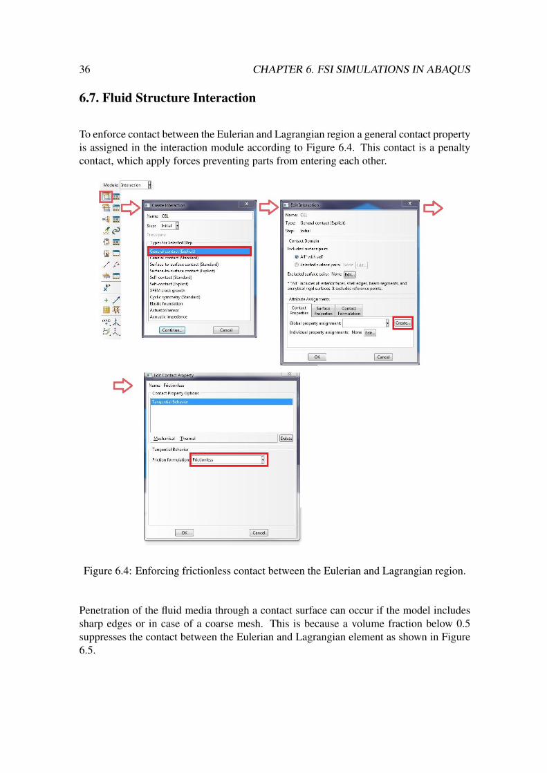
To enforce contact between the Eulerian and Lagrangian region a general contact propertyis assigned in the interaction module according to Figure 6.4. This contact is a penaltycontact, which apply forces preventing parts from entering each other.

Figure 6.4: Enforcing frictionless contact between the Eulerian and Lagrangian region.

Penetration of the fluid media through a contact surface can occur if the model includessharp edges or in case of a coarse mesh. This is because a volume fraction below 0.5suppresses the contact between the Eulerian and Lagrangian element as shown in Figure6.5.

6.8. BOUNDARY CONDITIONS AND LOADS 37

Figure 6.5: Left Figure shows penetration in a simple fluid structure interaction model.Right Figure shows that a volume fraction below 0.5 suppresses contact. [15]

6.8. Boundary Conditions and Loads

The standard boundary condition is free flow which allows the material to flow across theboundary freely. It also means that if a material is specified in contact with a boundary,the boundary will have free inflow of that material.

To prevent in or outflow over a boundary, the velocity can be prescribed to zero. Pre-scribed in (or outflow) can be defined in the same manner.

6.9. Submitting an Analysis Job

There are two ways of submitting a job. Either on a cluster or on the local computer. CELanalysis is very time consuming, thus it is highly recommended to use clusters.

As discussed earlier CEL analysis calculates a lot of time increments and because of thisit is recommended to use double precision for more accurate results.


6.10. Visualization

To visualize the fluid, choose to plot deformed contours: EVF_VOID. Then open theView Cut Manager and check the box EVF_VOID and set the value to 0.5. This willhide all elements not containing at least 50% fluid. In the result options set Averagingthreshold to 100% and open the common plot options > other > translucency and apply70% translucency. This will result in a clear visualization.

7. NUMERICAL TRANSVERSAL SEALING

SIMULATIONS IN ABAQUS

The intention of the work reported in this chapter is to show how to create a model ofthe transversal sealing process in Abaqus using the Coupled Eulerian-Lagrangian for-mulation, and to evaluate whether CEL is well suited for simulation of the TS process.Unfortunately there have been many obstacles in creating a realistic model of the sealingprocess which is why the first part of this chapter will discuss the limitations of analyzingthe TS process using CEL and Abaqus/Explicit in general.

7.1. Limitations

Much of what is enlightened here has also been raised in chapters 5 and 6 but is herediscussed as application specific.

The polymer layers that are studied has a thickness of about 50 µm . The layers arecompressed and due to this the thickness will decrease with time. In the real applicationthe polymer layer is often compressed until the thickness of the polymer layer is closeto zero. This means that using a Lagrangian mesh in an explicit solution is out of thequestion since the element length and thus the time increment would also tend to zero.

Using a Eulerian mesh solves the problem of decreasing element lengths since it is fixedin space through the analysis. Yet, the element length will be very small, considering thatthere must be at least two elements, preferably three or four in the thickness direction ofthe polymer layers to capture the behavior.

Problems with small time increments can usually be solved by introducing higher massin the system which increases the stable time increment cf. Chapter 6.1. The requirementfor such an assumption to not have large physical effects is that the material is not ratedependent, i.e. that the material model does not depend on velocities. Unfortunately allviscous media does. This means that introducing higher density when simulating fluidsusing CEL will result in exaggerated forces.

39

40 CHAPTER 7. TS SIMULATIONS IN ABAQUS

During the TS process the polymer undergoes phase transitions. First the polymer is insolid form and as the temperature reaches the melting point of the polymer it will changephase to fluid media. This process is then reversed as the sealing cools off.

To capture this in the computer analysis, the media would first have to be elastic and thentransform to viscous with temperature. Since temperature degrees of freedom is not yetavailable in CEL analysis this is not possible.

One must also be careful using high viscosities because of the impact on the computa-tional cost discussed in chapter 6.

Even though there are several obstacles in creating a realistic model of the TS process, amodel was created using a constant viscosity of 100 Pa s, mass scaling and a rough mesh.All which has been declared as unphysical in the above text.

7.2. Abaqus/CEL TS Model

The FSI model of the transversal sealing process was created using Abaqus/CAE 6.10-2with the implemented CEL formulation, cf Chapter 5.2 and 6.

Initially, the model was intended to be created solely as a Fluid Structure Interactionmodel using CEL. The polymer however can not be considered as a fluid during the entiretime period since polymers at low temperatures are elastic.

Therefore the sealing process will be modeled in two steps as indicated in Figure 7.1.In the first part the polymer will be modeled as a solid (Lagrangian part) with elasticbehavior, after which the deformed geometry from the solid phase simulation will beused as input to the fluid phase simulation. The polymer will be switched to an Eulerianpart and the analysis will be carried out using the CEL formulation.

This is a rough representation of the phase transition from solid to liquid behavior of thepolymer, and a major error may be introduced. This error is due to that the the deformedgeometry obtained from the solid simulation is stress free, but in reality this is not thecase. The latter part of the process, containing the unloading phase will not be consideredsince there has been found no way to transfer the Eulerian material positions back to aLagrangian geometry in Abaqus.

7.2. ABAQUS/CEL TS MODEL 41

Figure 7.1: Analysis divided into two parts. Solid phase(gray) and Fluid phase(turquoise).

7.2.1. Geometry

The only available element for Eulerian analysis is the EC3D8R element which is an eightnode, linear, 3D element with reduced integration which means that the model must bethree dimensional.

To decrease computational cost only a small strip of the seal geometry was consideredand due to symmetry, shown in Figure 7.2, only one half of the model was modelled.

Figure 7.2: Symmetry of the model.


The geometry of the three anvils were modeled as shown in Figure 7.3. Only the bottomface of the anvil was expected to be in contact with other parts and thus to further decreasethe computational cost, the anvils were modeled as discrete rigid bodies since negligibledeformations of the anvils was expected.

Figure 7.3: The three anvils are modeled as discrete rigid body shells.

The packaging material which consists of several layers, cf. chapter 2, was for simplicitymodeled as two layers, namely the paper and the polymer as shown in figure 7.4.

Figure 7.4: Simplified model of two opposite sheets of packaging material.


7.2.2. Simulation of the Solid Phase of the Polymer

The solid phase simulation is modeled according to Figure 7.5 where both the paper andpolymer are modelled as deformable (Lagrangian) parts. The constitutive behavior of thepaper is modeled using a simplified material model, which captures the compressionalbehavior of the paper. The material of the polymer is modeled as a linear isotropic materialwith Young’s modulus 200 MPa and the Poisson’s ratio has been set to zero for bothmaterials

Figure 7.5: FE-model of the solid phase of the polymer using anvil M1.

The symmetry boundary is modeled as a restricted motion in the x-direction. The horn isnot modelled, instead a prescribed boundary condition is applied representing the horn.The model has a boundary condition to the right which also is a restricted displacementin the x-direction. The whole model is also restricted in the z-direction as the modelrepresents a small slice of what is seen as a infinite long sealing. The displacement of theanvil is controlled by a reference point which is restricted in the z and x direction as wellas rotations and assigned a motion in the negative y direction according to Figure 7.6.The curve controlling this displacement is adopted from the measurements but has beensmoothed due to numerical stability issues.


Figure 7.6: Simplification of deformation curve from experimental testing.

The analysis was carried out at a loading rate that was increased by a factor of 100,preventing long analysis time. Frictionless general contact was prescribed between theanvil and the top paper. General contact uses penalties to enforce contact. This meansthat it applies a force which depends on the overclosure of the nodes. This means thatoverclosure will always occur. The default penalty was not strong enough and thus ascaling was required. A scaling of 9 times the default penalty seemed to be enough andwere used. The effects of using scaled penalties has not been studied in this work.

7.2.3. Simulation of the Fluid Phase of the Polymer

The geometry of the fluid phase simulation was extracted from the results of the Solidphase simulation. This was done by importing the deformed mesh from the odb file. InAbaqus, an imported mesh is called an orphan mesh and has few changeable attributes.By transforming the orphan mesh into a part using the Abaqus commands PartFromSec-tion3DMeshByPlane and Part2DGeomFrom2DMesh the orphan mesh is first transformedinto a 2D orphan mesh and then into a 2D shell part. By using the sketch from this part a3D deformable part can be created. The script file used for this can be found in AppendixB.1.


The fluid polymer was modeled as a material with a constant viscosity of 100 Pa s partlybecause temperature degrees of freedom is not yet implemented in CEL analysis andpartly because high viscosity models are very time consuming. The Cross-Arrheniusimplementation discussed in chapter 4 was not used but may be used in the next versionof Abaqus where temperature degrees of freedoms are introduced.

The boundary conditions for the fluid model was the same as in the solid phase simulationexcept that there was no tie between the paper and polymer since it was considered as afluid. Velocity boundary conditions in the x and z-direction have been set as symmetryconditions for the Eulerian region in accordance with chapter 6.

To reduce the analysis time, the actual process time was decreased by a factor of 10000.The analysis time was 5.5 minutes. The full scale model would occupy 8 cpus for 38 daysdespite all assumptions made. The contact penalty was scaled in the same way as in thesolid model.

In the analysis, the anvil was deformation controlled and a smoothed curve of the mea-sured deformations from the experiments was used as input, as shown in Figure 7.7.

Figure 7.7: Simplification of deformation curve from experimental testing.


The results from both the solid and the fluid analysis is shown in Figure 7.8.

Figure 7.8: Undeformed geometry and results from the solid and the fluid analysis.

8. CONCLUSIONS

Throughout this work, the main objective was to investigate whether the Coupled Eulerian-Lagrangian formulation implemented in Abaqus is well suited for simulating the full seal-ing process where the packaging material structure is compressed and heated.

In the journey towards this objective several important findings have been identified, es-pecially concerning material properties of polymer materials during the fluid phase.

It has been recognized that the viscosity is the primary material parameter to define theresistance of motion for the polymer material. A general method of fitting experimentaldata of shear rate and temperature dependent viscosity to a surface function using theCross and Arrhenius functions has been developed and the implementation in Abaqus bymeans of subroutines has also been discussed in the thesis.

Experimental work was made to achieve a better understanding of the sealing process,using ultra sonic vibrations, and also to obtain referential results for the analyses and forfuture work.

The experimental data shows that not only the polymer layer weakens due to heating butalso the paperboard layers. It also shows that the deformed geometry of the packagingmaterial, both polymer and paperboard is a direct consequence of the choice of anvil.

Much of the work in the thesis has been devoted to understanding how and if the CELformulation is suitable for transversal sealing process simulations.

The CEL formulation is a tool for analyzing fluid structure interaction by allowing contactconditions between Lagrangian and Eulerian regions. In other words, fluids can interactwith solids which was why the method was chosen by Tetra Pak for this thesis.

During the thesis several obstacles, which made it impossible to make a physically accu-rate analysis, were encountered.

The main problem was the time increment which tends to zero for very small geometriessuch as found in the sealing process. The problem is due to using an explicit solver.Explicit solvers needs small time increments for the solution to be numerically stable.When using CEL, there has been found no way around the problem other then scaling themass or size of the model, but this changes the results.

47

48 CHAPTER 8. CONCLUSIONS

There has neither been found a way to simulate the phase transition without changing thephysics of the process. At the very end of this work an idea of adding an elastic shearmodulus came up. Possibly, it is a way of solving the phase transition problem. Therewas however no time to investigate that possibility within the time frame of the thesis.

The general conclusion of this part of the thesis is that the limitations of the CEL formu-lation for small scale geometry, high viscosities or phase transitions is so critical that atthis time there has not been found a good way to simulate the full sealing process withoutcompromising the physics.

9. SUGGESTIONS FOR FURTHER WORK

Several findings were done during the FE-model development in this thesis. The materialmodel for the polymer needs further work. Ways of capturing the solid phase and the tran-sition between solid and fluid phase needs to be investigated. Further more experimentalverification of the fluid phase material model is needed.

To be able to create a realistic model of the sealing process using CEL the analysis mustbe carried out without scaling the time which would take roughly 38 days at 8cpu’s. Theproblem of small time increments must be solved otherwise, perhaps by scaling quantitieswith knowledge of how the physics is changing and compensate for this in the results.

Furthermore one should be able to implement the material model as soon as temperaturedegrees of freedom is introduced in Abaqus 6.11.

A material model for the thermal coupling should also be considered as the high temper-ature of the sealing process surely affects both the polymer and the paper.

Probably the best way of gaining knowledge of the sealing process and creating a realisticmodel is to take a step back and examine each subprocess of the sealing process separately.

As discussed earlier the material models needs to be further developed and verified. Alsoknowledge of how the heat is generated and transported in both the paperboard and thepolymer is needed.

When all subprocesses are known, the work of putting these together can be initiated.How the coupling should be done and by means of which software is also an issue ofinterest.

49

BIBLIOGRAPHY

[1] Tetra Pak homepage, Tetra pak in figures (Sept 2010). Available from:http://www.tetrapak.com

[2] Rheology school, Making Use Of Models (Oct 2010). Available from:http://www.rheologyschool.com/

[3] Internal Tetra Pak report.

[4] Belytschko T, Non Linear Continua Equations. 1998

[5] Johansson Consulting Six Sigma Black Belt Training.

[6] Holzapfel G.A, Nonlinear solid mechanics - A continuum approach for engineering.1998

[7] White F.M, Fluid Mechanics - Sixth Edition. 2008

[8] Price J.F, Lagrangian and Eulerian Representations of Fluid Flow: Kinematics andthe Equations of motion. 2006

[9] Ottosen N.S, Ristinmaa M, The Mechanics of Constitutive Modeling. 2005

[10] Krenk S, Non-Linear Modeling and Analysis of Solids and Structures. 2009

[11] Min Soo Kim, Woo Il Lee, A new VOF-based numerical scheme for the simulationof fluid flow with free surface. Part I: New free surface-tracking algorithm and itsverification. 2003

[12] Helleloid G.T, Morehead Electronic Journal of Applicable Mathematics, Issue 1 -CHEM-2000-01 On the Computation of Viscosity-Shear Rate Temperature MasterCurves for Polymeric Liquids. University of Wisconsin - Madison

[13] Polymer technology, Rheology of fluids (Sept 2010). Available from:http://polymer.w99of.com

[14] Dassault Systemes Simulia Corp, Abaqus Manual, Version 6.10. 2010

[15] Dassault Systemes Simulia Corp, Abaqus/Explicit: Advanced Topics & CoupledEulerian-Lagrangian Analysis. Presented at Tetra Pak, Lund, October 6-9 2008

51

52 BIBLIOGRAPHY

[16] Dassault Systemes Simulia Corp, Answer ID 3765 available from Abaqus support.

[17] Dassault Systemes Simulia Corp, Answer ID 4466 available from Abaqus support.2010

[18] Dassault Systemes Simulia Corp, Answer ID 3523 available from Abaqus support.2010

[19] Sharat Prasad, Engineering Specialist, Dassault Systemes. 13 October, 2010

[20] Pacific Northwest National Laboratory, Available from: http://www.technet.pnl.gov

A. ABAQUS INPUT FILES

A.1. Solid Model Input File

*Heading** Job name: TS_solid_P1_M1 Model name: Model-1** Generated by: Abaqus/CAE 6.10-2*Preprint, echo=NO, model=NO, history=NO, contact=NO**** PARTS***Part, name=Anvil*End Part***Part, name=Anvil-disp*End Part***Part, name="Bottom paper"*End Part***Part, name="Eulerian region"*End Part***Part, name="Eulerian region-2"*End Part***Part, name="Top paper"*End Part****** ASSEMBLY***Assembly, name=Assembly***Instance, name="Bottom paper-1", part="Bottom paper"*Node

1, 0.000899999985, 0., 0....3618, 0.000950000016, 4.99999987e-05, 0.*Element, type=C3D8R1, 94, 102, 966, 847, 1, 2, 13, 46

...1600, 102, 2, 1, 94, 2351, 846, 485, 3618*Nset, nset=paperboundary

1, 2, 10, 11, 485, 486, 487, 488, 489, 490, 491, 492, 493, 494, 495, 496...833, 834, 835, 836, 837, 838, 839, 840, 841, 842, 843, 844, 845, 846

*Elset, elset=paperboundary, generate152, 1600, 8

** Section: Hyperfoam*Solid Section, elset=_paper_part, material=Hyperfoam,

53

54 APPENDIX A. ABAQUS INPUT FILES

*End Instance***Instance, name="Eulerian region-1", part="Eulerian region"-2.76471553983809e-20, 0.000150000000000003, 0.

*Node1, 0.00999999978, 0.000349999988, 2.49999994e-05

...4008, 0., 0.000300000014, 0.

*Element, type=C3D8R1, 9, 10, 14, 13, 1, 2, 6, 5

...1500, 4003, 4004, 4008, 4007, 3995, 3996, 4000, 3999** Section: Plastic*Solid Section, elset=_polymer_part, material=Plastic,*End Instance***Instance, name="Top paper-1", part="Top paper"

0., 0.000499999999999999, 0.*Node

1, 0.00999999978, 0.00039999999, 2.49999994e-05...

3618, 0., 0., 0.*Element, type=C3D8R

1, 19, 20, 29, 28, 1, 2, 11, 10...1600, 3608, 3609, 3618, 3617, 3590, 3591, 3600, 3599*End Instance***Instance, name="Eulerian region-2-1", part="Eulerian region-2"

0., 0.000100000000000001, 0.*Node

1, 0.00999999978, 0.000349999988, 2.49999994e-05...24024, 0., 0.000300000014, 0.

*Element, type=C3D8R1, 25, 26, 32, 31, 1, 2, 8, 7

...15000, 24017, 24018, 24024, 24023, 23993, 23994, 24000, 23999** Section: Plastic*Solid Section, elset=_polymer_part_2, material=Plastic,*End Instance***Instance, name=Anvil-1, part=Anvil0.00044764297739604, 0.00279741988391855, 0.*Node

1, 0.00180235703, -0.00179741986, 2.49999994e-05...

288, 0.00185235706, -0.00171081733, 0.*Element, type=R3D41, 1, 23, 26, 4...143, 286, 1, 4, 287*Node

289, 0.00170235697, -0.00189741992, 2.49999994e-05*Nset, nset=Anvil-1-RefPt_, internal289,*Elset, elset=Anvil-1, generate

1, 143, 1*End Instance***Instance, name=Anvil-disp-1, part=Anvil-disp0.00044764297739604, 0.00279741988391855, 0.*Node

1, 0.00179474498, -0.00183568825, 2.49999994e-05...

A.1. SOLID MODEL INPUT FILE 55

110, 0.00260235695, -0.00169741991, 0.*Element, type=S31, 10, 4, 9

...84, 108, 106, 107*End Instance***Nset, nset=_PickedSet48, internal, instance="Bottom paper-1"

3, 4, 6, 7, 9, 10, 11, 12, 81, 82, 83, 84, 85, 86, 87, 95...119, 120, 121, 122

*Nset, nset=_PickedSet48, internal, instance="Top paper-1"1, 2, 3, 4, 5, 6, 7, 8, 9, 10, 11, 12, 13, 14, 15, 16

...3615, 3616, 3617, 3618

*Elset, elset=_PickedSet48, internal, instance="Bottom paper-1"18, 36, 54, 72, 90, 108, 126, 144, 145, 146, 147, 148, 149, 150, 151, 152

*Elset, elset=_PickedSet48, internal, instance="Top paper-1"1, 2, 3, 4, 5, 6, 7, 8, 1593, 1594, 1595, 1596, 1597, 1598, 1599, 1600

*Nset, nset=_PickedSet98, internal, instance="Eulerian region-1"1, 2, 3, 4, 5, 6, 7, 8, 4001, 4002, 4003, 4004, 4005, 4006, 4007, 4008

*Nset, nset=_PickedSet98, internal, instance="Eulerian region-2-1"1, 2, 3, 4, 5, 6, 7, 8, 9, 10, 11, 12, 13, 14, 15, 16

...24009, 24010, 24011, 24012, 24013, 24014, 24015, 24016, 24017, 24018, 24019, 24020, 24021, 24022, 24023, 24024

*Elset, elset=_PickedSet98, internal, instance="Eulerian region-1"1, 2, 3, 1498, 1499, 1500

*Elset, elset=_PickedSet98, internal, instance="Eulerian region-2-1"1, 2, 3, 4, 5, 6, 7, 8, 9, 10, 11, 12, 13, 14, 15, 14986

14987, 14988, 14989, 14990, 14991, 14992, 14993, 14994, 14995, 14996, 14997, 14998, 14999, 15000*Nset, nset=_PickedSet99, internal, instance="Eulerian region-1"

1, 2, 3, 4, 6, 7, 8, 9, 10, 11, 12, 14, 15, 16, 17, 18...4006, 4007, 4008

*Nset, nset=_PickedSet99, internal, instance="Eulerian region-2-1"1, 2, 3, 4, 5, 6, 19, 20, 21, 22, 23, 24, 25, 26, 27, 28

...24001, 24002, 24003, 24004, 24005, 24006, 24019, 24020, 24021, 24022, 24023, 24024

*Elset, elset=_PickedSet99, internal, instance="Eulerian region-1", generate1, 1500, 1

*Elset, elset=_PickedSet99, internal, instance="Eulerian region-2-1"1, 2, 3, 4, 5, 11, 12, 13, 14, 15, 16, 17, 18, 19, 20, 26

...14975, 14981, 14982, 14983, 14984, 14985, 14986, 14987, 14988, 14989, 14990, 14996, 14997, 14998, 14999, 15000

*Nset, nset=_PickedSet122, internal, instance="Bottom paper-1"1, 2, 10, 11, 485, 486, 487, 488, 489, 490, 491, 492, 493, 494, 495, 496

...833, 834, 835, 836, 837, 838, 839, 840, 841, 842, 843, 844, 845, 846

*Elset, elset=_PickedSet122, internal, instance="Bottom paper-1", generate152, 1600, 8

*Nset, nset=_PickedSet123, internal, instance="Bottom paper-1", generate1, 3618, 1

*Nset, nset=_PickedSet123, internal, instance="Top paper-1", generate1, 3618, 1

*Elset, elset=_PickedSet123, internal, instance="Bottom paper-1", generate1, 1600, 1

*Elset, elset=_PickedSet123, internal, instance="Top paper-1", generate1, 1600, 1

*Nset, nset=_PickedSet132, internal, instance=Anvil-1289,

*Elset, elset=__PickedSurf108_S4, internal, instance="Eulerian region-2-1", generate5, 15000, 5

*Surface, type=ELEMENT, name=_bottompolymer_tie, internal__PickedSurf108_S4, S4*Elset, elset=__PickedSurf109_S4, internal, instance="Top paper-1", generate

8, 1600, 8*Surface, type=ELEMENT, name=_toppaper_tie, internal


__PickedSurf109_S4, S4*Elset, elset=__PickedSurf110_S6, internal, instance="Eulerian region-1", generate

1, 1498, 3*Surface, type=ELEMENT, name=_toppolymer_tie, internal__PickedSurf110_S6, S6*Elset, elset=__PickedSurf140_S6, internal, instance="Bottom paper-1", generate145, 1593, 8

*Elset, elset=__PickedSurf140_S1, internal, instance="Bottom paper-1", generate127, 144, 1

*Surface, type=ELEMENT, name=_bottompaper_tie, internal__PickedSurf140_S6, S6__PickedSurf140_S1, S1*Elset, elset=_Surf-1_S4, internal, instance="Eulerian region-1", generate

3, 1500, 3*Surface, type=ELEMENT, name=Surf-1_Surf-1_S4, S4*Elset, elset=_Surf-2_S6, internal, instance="Eulerian region-2-1", generate

1, 14996, 5*Surface, type=ELEMENT, name=Surf-2_Surf-2_S6, S6*Rigid Body, ref node=Anvil-1.Anvil-1-RefPt_, elset=Anvil-1.Anvil-1** Constraint: Bottom_tie*Tie, name=Bottom_tie, adjust=yes_bottompolymer_tie, _bottompaper_tie** Constraint: Top_Tie*Tie, name=Top_Tie, adjust=yes_toppolymer_tie, _toppaper_tie** Constraint: disp_body*Display Body, instance=Anvil-disp-1Anvil-1.289,*End Assembly*Amplitude, name=Amp-2, definition=SMOOTH STEP

0., 0., 0.0007, 0.00022, 0.00285, 0.00028, 0.00333, 0.00047**** MATERIALS***Material, name=Hyperfoam*Density100000.,** (Massscaled)*Hyperfoam, testdata*Uniaxial Test Data

4.48e+07, 0.6, 0.-5.143e+06, -0.1, 0.-1.1174e+07, -0.15, 0.-2.3047e+07, -0.25, 0.-3.918e+07, -0.3, 0.-5.8665e+07, -0.35, 0.-7.8569e+07, -0.38, 0.

-1.06656e+08, -0.42, 0.-2.17907e+08, -0.5, 0.-4.54272e+08, -0.6, 0.

*Material, name="Linear elastic"*Density100000.,** (Massscaled)*Elastic3e+08,0.

*Material, name=Plastic*Density100000.,** (Massscaled)*Elastic2e+08,0.

**** INTERACTION PROPERTIES**

A.1. SOLID MODEL INPUT FILE 57

*Surface Interaction, name=general**** BOUNDARY CONDITIONS**** Name: Euelrian X-led Type: Displacement/Rotation*Boundary_PickedSet98, 1, 1** Name: Euelrian Z-led Type: Displacement/Rotation*Boundary_PickedSet99, 3, 3** Name: Lagr_X-led Type: Displacement/Rotation*Boundary_PickedSet48, 1, 1** Name: Lagr_Y-led Type: Displacement/Rotation*Boundary_PickedSet122, 2, 2** Name: Lagr_Z-led Type: Displacement/Rotation*Boundary_PickedSet123, 3, 3** ----------------------------------------------------------------**** STEP: dyn_expl***Step, name=dyn_expl*Dynamic, Explicit, 0.00333*Bulk Viscosity0., 0.**** BOUNDARY CONDITIONS**** Name: Rigid_body_motion Type: Displacement/Rotation*Boundary, amplitude=Amp-2_PickedSet132, 1, 1_PickedSet132, 2, 2, -1._PickedSet132, 3, 3_PickedSet132, 4, 4_PickedSet132, 5, 5_PickedSet132, 6, 6**** INTERACTIONS**** Interaction: Int-1*Contact, op=NEW*Contact Inclusions, ALL EXTERIOR*Contact Property Assignment, , general

*Contact controls assignment, type=scale penaltysurf-1,surf-2,9**** OUTPUT REQUESTS***Restart, write, number interval=1, time marks=NO**** FIELD OUTPUT: F-Output-1***Output, field, variable=PRESELECT, number interval=100**** HISTORY OUTPUT: Energy***Output, history*Energy OutputALLAE, ALLCD, ALLCW, ALLDC, ALLDMD, ALLFD, ALLIE, ALLKE, ALLMW, ALLPD, ALLPW, ALLSE, ALLVD, ALLWK, ETOTAL*End Step


A.2. Liquid Model Input File

*Heading** Job name: TS_visc_P1_M1 Model name: Model-1** Generated by: Abaqus/CAE 6.10-2*Preprint, echo=NO, model=NO, history=NO, contact=NO**** PARTS***Part, name=Anvil*End Part***Part, name=Anvil-disp*End Part***Part, name="Bottom Paper"*End Part***Part, name=Eulerian*Surface, type=EULERIAN MATERIAL, name=polymer-1polymer-1*End Part***Part, name="Top Paper"*End Part****** ASSEMBLY***Assembly, name=Assembly***Instance, name=Anvil-1, part=Anvil0.00044764297739604, 0.00248640988391855, 0.*Node

1, 0.00180235703, -0.00179741986, 2.49999994e-05...

856, 0.00188284798, -0.00169934134, 0.*Element, type=R3D41, 1, 23, 36, 4...427, 849, 1, 4, 850*Node

857, 0.00170235697, -0.00189741992, 2.49999994e-05*Nset, nset=Anvil-1-RefPt_, internal857,*Elset, elset=Anvil-1, generate

1, 427, 1*End Instance***Instance, name=Anvil-disp-1, part=Anvil-disp0.00044764297739604, 0.00248640988391855, 0.*Node

1, 0.00179474498, -0.00183568825, 2.49999994e-05...

110, 0.00260235695, -0.00169741991, 0.*Element, type=S31, 10, 4, 9

...84, 108, 106, 107*End Instance***Instance, name="Bottom Paper-1", part="Bottom Paper"*Node

1, 0.00701939687, 0., 0....

A.2. LIQUID MODEL INPUT FILE 59

3842, 0.006480732, 0.00016022168, 2.99999992e-05*Element, type=C3D8R

1, 922, 694, 244, 243, 2843, 2615, 2165, 2164...1713, 1886, 1449, 1920, 1921, 3807, 3370, 3841, 3842** Section: Paper_sect*Solid Section, elset=_PickedSet4, material="Linear elastic",*End Instance***Instance, name="Top Paper-1", part="Top Paper"*Node

1, 0.00875478052, 0.000619949307, 0....

3766, 0.000673354371, 0.00057974353, 2.99999992e-05*Element, type=C3D8R

1, 692, 3, 1, 691, 2575, 1886, 1884, 2574...1674, 1312, 1882, 1640, 414, 3195, 3765, 3523, 2297** Section: Paper_sect*Solid Section, elset=_PickedSet4, material="Linear elastic",*End Instance***Instance, name=Eulerian, part=Eulerian

0.005125, 0.00113899, 0.*Node

1, -0.00512500014, -0.00100000005, 2.99999992e-05...14028, 0.0048750001, -0.00039999999, 0.

*Element, type=EC3D8R1, 43, 44, 65, 64, 1, 2, 23, 22

..2607, 2608, 2609, 2610, 2611, 2612, 2613, 2614

*Elset, elset=_PickedSet231, internal, instance="Bottom Paper-1"10, 11, 12, 13, 34, 36, 39, 40, 41, 42, 43, 44, 54, 55, 56, 57

...1061, 1074, 1082

*Nset, nset=_PickedSet232, internal, instance="Bottom Paper-1", generate1, 3842, 1

*Nset, nset=_PickedSet232, internal, instance="Top Paper-1", generate1, 3766, 1

*Elset, elset=_PickedSet232, internal, instance="Bottom Paper-1", generate1, 1713, 1

*Elset, elset=_PickedSet232, internal, instance="Top Paper-1", generate1, 1674, 1

*Nset, nset=_PickedSet238, internal, instance=Eulerian1, 2, 3, 4, 5, 6, 7, 8, 9, 10, 11, 12, 13, 14, 15, 16

...14025, 14026, 14027, 14028

*Elset, elset=_PickedSet238, internal, instance=Eulerian1, 2, 3, 4, 5, 6, 7, 8, 9, 10, 11, 12, 13, 14, 15, 16

17, 18, 19, 20, 6641, 6642, 6643, 6644, 6645, 6646, 6647, 6648, 6649, 6650, 6651, 66526653, 6654, 6655, 6656, 6657, 6658, 6659, 6660

*Nset, nset=_PickedSet239, internal, instance=Eulerian, generate1, 14028, 1

*Elset, elset=_PickedSet239, internal, instance=Eulerian, generate1, 6660, 1

*Nset, nset=_PickedSet240, internal, instance=Anvil-1857,


*Elset, elset=_PickedSet268, internal, instance=Eulerian, generate1, 6660, 1


*Elset, elset=_PickedSet273, internal, instance=Eulerian, generate


1, 6660, 1*Nset, nset=_PickedSet274, internal, instance=Eulerian, generate

1, 14028, 1*Elset, elset=_PickedSet274, internal, instance=Eulerian, generate

1, 6660, 1*Nset, nset=_PickedSet275, internal, instance=Eulerian, generate

1, 14028, 1*Elset, elset=_PickedSet275, internal, instance=Eulerian, generate

1, 6660, 1*Nset, nset=_PickedSet276, internal, instance=Eulerian

1, 21, 22, 42, 43, 63, 64, 84, 85, 105, 106, 126, 127, 147, 148, 168...13945, 13965, 13966, 13986, 13987, 14007, 14008, 14028

*Elset, elset=_PickedSet276, internal, instance=Eulerian1, 20, 21, 40, 41, 60, 61, 80, 81, 100, 101, 120, 121, 140, 141, 160

...6561, 6580, 6581, 6600, 6601, 6620, 6621, 6640, 6641, 6660

*Elset, elset=_Surf-1_SPOS, internal, instance=Anvil-1, generate1, 427, 1

*Surface, type=ELEMENT, name=Surf-1_Surf-1_SPOS, SPOS*Elset, elset=_Surf-2_S4, internal, instance="Top Paper-1"

4, 5, 9, 11, 12, 15, 20, 30, 43, 44, 46, 47, 65, 68, 70, 71...941, 962, 966, 995, 1033, 1367

*Elset, elset=_Surf-2_S6, internal, instance="Top Paper-1"7, 8, 10, 14, 17, 19, 22, 24, 26, 27, 28, 29, 31, 32, 33, 67

...403, 406, 409, 491, 493, 494, 495, 497, 565, 693, 796, 827, 876, 887

*Elset, elset=_Surf-2_S5, internal, instance="Top Paper-1"35, 116, 130, 216, 219, 221, 367, 392, 411, 415, 431, 443, 445, 450, 461, 463999, 1001, 1002, 1013, 1016, 1018, 1022, 1025, 1026


...577, 751, 803, 804, 824, 908, 939, 1000, 1019, 1032, 1055

*Surface, type=ELEMENT, name=Surf-2_Surf-2_S4, S4_Surf-2_S6, S6_Surf-2_S5, S5_Surf-2_S3, S3*Elset, elset=_Surf-3_S4, internal, instance="Top Paper-1"

1, 37, 39, 52, 53, 54, 55, 57, 58, 62, 79, 82, 102, 104, 180, 194...976, 978, 980, 982, 990, 1043, 1045, 1049, 1626


...544, 545, 546, 547, 549, 550, 551, 689, 715, 721, 724, 838

*Elset, elset=_Surf-3_S5, internal, instance="Top Paper-1"59, 932, 984

*Surface, type=ELEMENT, name=Surf-3_Surf-3_S4, S4_Surf-3_S6, S6_Surf-3_S5, S5*Elset, elset=_Surf-4_S6, internal, instance="Bottom Paper-1"223, 269, 306, 317, 343, 353, 354, 355, 356, 357, 365, 814, 994, 1692

*Elset, elset=_Surf-4_S4, internal, instance="Bottom Paper-1"221, 304, 305, 307, 314, 315, 316, 318, 342, 351, 352, 361, 362, 364, 366, 561996,

*Elset, elset=_Surf-4_S3, internal, instance="Bottom Paper-1"19, 20, 21, 23, 25, 28, 29, 30, 31, 48, 49, 70, 82, 87, 89, 92

...1017, 1019, 1024, 1029, 1046

*Elset, elset=_Surf-4_S5, internal, instance="Bottom Paper-1"1, 3, 4, 6, 17, 27, 68, 69, 75, 76, 81, 86, 88, 90, 91, 102

...

A.2. LIQUID MODEL INPUT FILE 61

476, 480, 482, 757*Surface, type=ELEMENT, name=Surf-4_Surf-4_S6, S6_Surf-4_S4, S4_Surf-4_S3, S3_Surf-4_S5, S5*Rigid Body, ref node=Anvil-1.Anvil-1-RefPt_, elset=Anvil-1.Anvil-1** Constraint: disp_body*Display Body, instance=Anvil-disp-1Anvil-1.857,*End Assembly**** ELEMENT CONTROLS***Section Controls, name=EC-1, hourglass=VISCOUS0., 1., 1., 0., 0.*Amplitude, name=Amp-1, definition=SMOOTH STEP

0., 0., 1.5e-05, 0.0002**** MATERIALS***Material, name=Hyperfoam*Density100000.,** (Massscaled 100 times)*Hyperfoam, testdata*Uniaxial Test Data

4.48e+07, 0.6, 0.-5.143e+06, -0.1, 0.-1.1174e+07, -0.15, 0.-2.3047e+07, -0.25, 0.-3.918e+07, -0.3, 0.-5.8665e+07, -0.35, 0.-7.8569e+07, -0.38, 0.

-1.06656e+08, -0.42, 0.-2.17907e+08, -0.5, 0.-4.54272e+08, -0.6, 0.

*Material, name="Linear elastic"*Density100000.,** (Massscaled 100 times)*Elastic3e+08,0.

*Material, name=Plastic*Density1000.,*Elastic2e+08, 0.4

*Material, name=Polymer*Density1000.,*Eos, type=USUP1500.,0.,0.*Viscosity100.,**** INTERACTION PROPERTIES***Surface Interaction, name=general**** BOUNDARY CONDITIONS**** Name: Euler_X-led Type: Velocity/Angular velocity*Boundary, type=VELOCITY_PickedSet238, 1, 1** Name: Euler_Z-led Type: Velocity/Angular velocity*Boundary, type=VELOCITY


_PickedSet239, 3, 3** Name: Eulerian-y Type: Velocity/Angular velocity*Boundary, type=VELOCITY_PickedSet276, 2, 2** Name: Lagr_X-led Type: Displacement/Rotation*Boundary_PickedSet230, 1, 1** Name: Lagr_Y-led Type: Displacement/Rotation*Boundary_PickedSet231, 2, 2** Name: Lagr_Z-led Type: Displacement/Rotation*Boundary_PickedSet232, 3, 3**** PREDEFINED FIELDS**** Name: Polyinit Type: Material assignment*Initial Conditions, type=VOLUME FRACTION** ----------------------------------------------------------------**** STEP: dyn_expl***Step, name=dyn_expl*Dynamic, Explicit, 1.5e-05*Bulk Viscosity0., 0.**** BOUNDARY CONDITIONS**** Name: Rigid_body_motion Type: Displacement/Rotation*Boundary, amplitude=Amp-1_PickedSet240, 1, 1_PickedSet240, 2, 2, -1._PickedSet240, 3, 3_PickedSet240, 4, 4_PickedSet240, 5, 5_PickedSet240, 6, 6**** INTERACTIONS**** Interaction: Int-1*Contact, op=NEW*Contact Inclusions, ALL EXTERIOR*Contact Property Assignment, , general

*Contact controls assignment, type=scale penaltysurf-1,surf-2,9**** OUTPUT REQUESTS***Restart, write, number interval=1, time marks=NO**** FIELD OUTPUT: F-Output-1***Output, field, variable=PRESELECT, number interval=100**** HISTORY OUTPUT: Energy***Output, history*Energy OutputALLAE, ALLCD, ALLCW, ALLDC, ALLDMD, ALLFD, ALLIE, ALLKE, ALLMW, ALLPD, ALLPW, ALLSE, ALLVD, ALLWK, ETOTAL*End Step

B. ABAQUS SCRIPT FILES IN PYTHON

B.1. Orphan Mesh to 3D Deformable Part

################################### BOTTOM PAPER-1 ##############from abaqus import *from abaqusConstants import *from caeModules import *## 3d Orphan to 2d Orphanmdb.models[’Model-1’].PartFromSection3DMeshByPlane(’BOTTOM PAPER-2’,mdb.models[’Model-1’].parts[’BOTTOM PAPER-1’],(0,0,1e-5),(0,0,1),(1,0,0))## 2d Orphan to Shell geometrymdb.models[’Model-1’].Part2DGeomFrom2DMesh(’BOTTOM PAPER-3’,mdb.models[’Model-1’].parts[’BOTTOM PAPER-2’],0)## Open sketchp = mdb.models[’Model-1’].parts[’BOTTOM PAPER-3’]s1 = p.features[’Shell planar-1’].sketchmdb.models[’Model-1’].ConstrainedSketch(name=’__edit__’, objectToCopy=s1)## Save sketchs2 = mdb.models[’Model-1’].sketches[’__edit__’]g, v, d, c = s2.geometry, s2.vertices, s2.dimensions, s2.constraintss2.setPrimaryObject(option=SUPERIMPOSE)p.projectReferencesOntoSketch(sketch=s2,

upToFeature=p.features[’Shell planar-1’], filter=COPLANAR_EDGES)mdb.models[’Model-1’].ConstrainedSketch(name=’Bottom Paper’, objectToCopy=s2)s2.unsetPrimaryObject()del mdb.models[’Model-1’].sketches[’__edit__’]## Create 3d deformable parts = mdb.models[’Model-1’].ConstrainedSketch(name=’__profile__’, sheetSize=0.01)g, v, d, c = s.geometry, s.vertices, s.dimensions, s.constraintss.sketchOptions.setValues(decimalPlaces=4)s.setPrimaryObject(option=STANDALONE)## Use sketchs.retrieveSketch(sketch=mdb.models[’Model-1’].sketches[’Bottom Paper’])p = mdb.models[’Model-1’].Part(name=’Bottom Paper’, dimensionality=THREE_D,

type=DEFORMABLE_BODY)p = mdb.models[’Model-1’].parts[’Bottom Paper’]p.BaseSolidExtrude(sketch=s, depth=3.333333e-5)s.unsetPrimaryObject()del mdb.models[’Model-1’].parts[’BOTTOM PAPER-1’]del mdb.models[’Model-1’].parts[’BOTTOM PAPER-2’]del mdb.models[’Model-1’].parts[’BOTTOM PAPER-3’]############################################################################

63

C. ABAQUS SUBROUTIN IN FORTRAN

C.1. VUVISCOSITY using Cross-Arrhenius Viscosity

subroutine vuviscosity (C Read only -

* nblock,* jElem, kIntPt, kLayer, kSecPt,* stepTime, totalTime, dt, cmname,* nstatev, nfieldv, nprops,* props, tempOld, tempNew, fieldOld, fieldNew,* stateOld,* shrRate,

C Write only -* viscosity,* stateNew )

Cinclude ’vaba_param.inc’

Cdimension props(nprops),

* tempOld(nblock),* fieldOld(nblock,nfieldv),* stateOld(nblock,nstatev),* shrRate(nblock),* tempNew(nblock),* fieldNew(nblock,nfieldv),* viscosity(nblock),* stateNew(nblock,nstatev)

Ccharacter*80 cmname

CC VARIABLESCn0 = 2950n = 0.58lambda = 2.3E0 = 45580R = 8.31434absZero = -273refTemp = 150Tmax = 300heatTime = 0.2coolTime = 0.3roomTemp = 20coolTemp = -180maxVisc = 200CC VISCOSITY SET ELEMENT WISE.Cdo k = 1, nblockCC HEATINGPHASE linear equation T=(Tmax-Roomtemp)/heattime*stepTime+RoomtempC

65

66 APPENDIX C. ABAQUS SUBROUTIN IN FORTRAN

if stepTime < heatTime thentest = (n0/(1+(lamda*shrRate(k)/exp(((E0/R)*(1/(refTemp-absZero)-1/((Tmax-roomTemp)/heatTime*stepTime+roomTemp-absZero)))))**(1-n)))*(1/exp(((E0/R)*(1/(refTemp-absZero)-1/((Tmax-roomTemp)/heatTime*stepTime+roomTemp-absZero)))))CC MAXIMUM VISCOSITY CHECK, BECAUSE OF VISCOSITYS INPACT ON THE TIME INCREMENTCif test > maxVisc thenviscosity(k) = maxViscelseviscosity(k) = testend ifCC COOLINGPHASE linear equation T=Tmax+Cooltemp/cooltime*(stepTime-heattime)Celse if stepTime < heatTime thenviskosity(k)= (n0/(1+(lamda*shrRate(k)/exp(((E0/R)*(1/(refTemp-absZero)-1/(Tmax+coolTemp/coolTime*(stepTime-heatTime)-absZero)))))**(1-n)))*(1/exp(((E0/R)*(1/(refTemp-absZero)-1/(Tmax+coolTemp/coolTime*(stepTime-heatTime)-absZero)))))CC MAXIMUM VISCOSITY CHECK, BECAUSE OF VISCOSITYS IMPACT ON THE TIME INCREMENTCif test > maxVisc thenviscosity(k) = maxViscelseviscosity(k) = testend ifend ifend doC

returnend

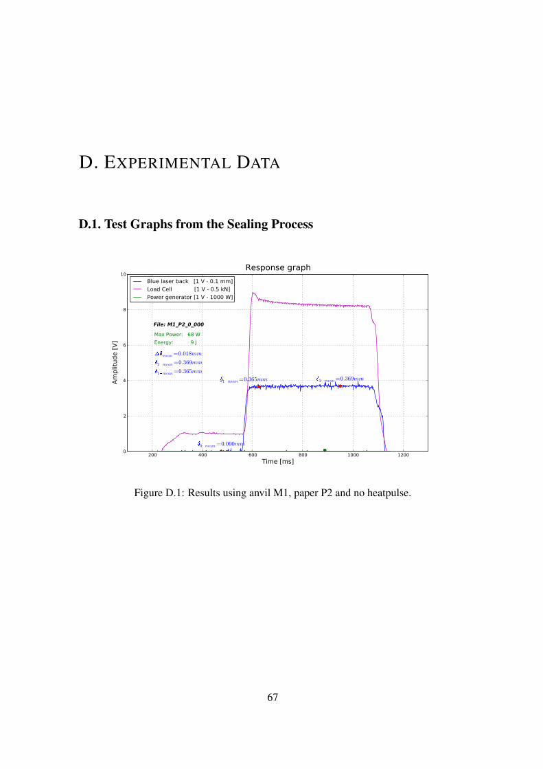
D. EXPERIMENTAL DATA

D.1. Test Graphs from the Sealing Process

200 400 600 800 1000 1200

Time [ms]

0

2

4

6

8

10

Am

plit

ude [

V]

Max Power: 68 W

Energy: 9 J

�2�mean=0.369mm

�0�mean=0.000mm

�1�mean=0.365mm

��mean=0.018mm�2�mean=0.369mm�1�mean=0.365mm

File: M1_P2_0_000

Response graph

Blue laser back [1 V - 0.1 mm]

Load Cell [1 V - 0.5 kN]

Power generator [1 V - 1000 W]

Figure D.1: Results using anvil M1, paper P2 and no heatpulse.

67

68 APPENDIX D. EXPERIMENTAL DATA

200 400 600 800 1000 1200

Time [ms]

0

2

4

6

8

10A

mplit

ude [

V]

Max Power: 1204 W

Energy: 32 J

�2�mean=0.355mm

�0�mean=0.000mm

�1�mean=0.322mm


File: M1_P2_1_030

Response graph




Figure D.2: Results using anvil M1, paper P2 and a 30 ms heatpulse.

200 400 600 800 1000 1200

Time [ms]

0

2

4

6

8

10

Am

plit

ude [

V]

Max Power: 2653 W

Energy: 103 J �2�mean=0.434mm

�0�mean=0.013mm

�1�mean=0.346mm


File: M1_P2_1_060

Response graph





D.1. TEST GRAPHS FROM THE SEALING PROCESS 69

200 400 600 800 1000 1200

Time [ms]

0

2

4

6

8

10A

mplit

ude [

V]

Max Power: 2915 W


�0�mean=0.000mm

�1�mean=0.359mm


File: M1_P2_1_090

Response graph





200 400 600 800 1000 1200

Time [ms]

0

2

4

6

8

10

Am

plit

ude [

V]

Max Power: 3071 W


�0�mean=0.002mm

�1�mean=0.363mm


File: M1_P2_1_120

Response graph






200 400 600 800 1000 1200

Time [ms]

0

2

4

6

8

10A

mplit

ude [

V]

Max Power: 3069 W

Energy: 371 J�2�mean=0.583mm

�0�mean=0.001mm

�1�mean=0.365mm


File: M1_P2_1_150

Response graph





200 400 600 800 1000 1200

Time [ms]

0

2

4

6

8

10

Am

plit

ude [

V]

Max Power: 3325 W

Energy: 396 J

�2�mean=0.594mm

�0�mean=0.091mm

�1�mean=0.373mm


File: M1_P1_1_150

Response graph





D.1. TEST GRAPHS FROM THE SEALING PROCESS 71

200 400 600 800 1000 1200

Time [ms]

0

2

4

6

8

10A

mplit

ude [

V]

Max Power: 2840 W

Energy: 328 J

�2�mean=0.743mm

�0�mean=0.205mm

�1�mean=0.557mm��mean=0.184mm�

2�mean=0.743mm�1�mean=0.557mm

File: M2_P1_1_150

Response graph





200 400 600 800 1000 1200

Time [ms]

0

2

4

6

8

10

Am

plit

ude [

V]

Max Power: 3126 W

Energy: 352 J

�2�mean=0.662mm

�0�mean=0.175mm



File: M2_P2_1_150

Response graph






200 400 600 800 1000 1200

Time [ms]

0

2

4

6

8

10A

mplit

ude [

V]

Max Power: 2682 W

Energy: 296 J

�2�mean=0.726mm

�0�mean=0.374mm



File: M3_P1_1_150

Response graph





200 400 600 800 1000 1200

Time [ms]

0

2

4

6

8

10

Am

plit

ude [

V]

Max Power: 2613 W

Energy: 290 J

�2�mean=0.696mm

�0�mean=0.329mm



File: M3_P2_1_150

Response graph





polymer flow in package sealing process - … flow in package ... 6 fluid structure interaction...

Documents