policy invariance under reward transformations: theory...
TRANSCRIPT

Policy Invariance Under Reward Transformations: Theory and Application to Reward Shaping
Paper by Andrew Ng, Daishi Harada, Stuart RussellPresentation by Kristin Branson
April 9, 2002

Reinforcement Learning
The reinforcement learning (RL) task: Learn the best action to take in any situation to maximize the total rewards earned.The agent learns which actions to take by interacting with its environment.

Markov Decision Processes (MDP)
In an MDP, the environment is represented as a Finite State Automaton with which the agent interacts in discrete episodes. All information relevant to which action to take is in the environment’s state (the Markov Property). M = (S, A, T = {Psa(s’)}, γ, R):
S is the set of states of the environment.A is the set of actions the agent can take.Psa(s’) is the probability s’ is the state after state s and action a. γ is the discount factor.R is the immediate reward function.
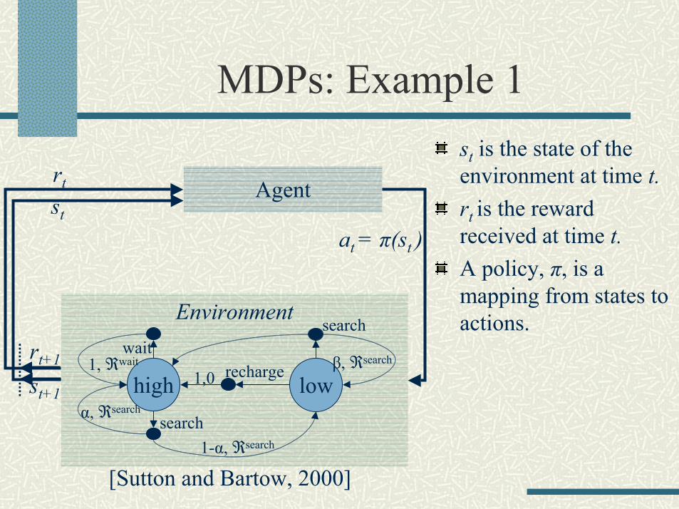
MDPs: Example 1st is the state of the environment at time t.rt is the reward received at time t.A policy, π, is a mapping from states to actions.
rt Agent
at = π(st )
rt+1
st+1
st
Environment
high lowrecharge
search1-α, ℜsearch
α, ℜsearch
wait1, ℜwait
search
1,0β, ℜsearch
[Sutton and Bartow, 2000]

Example: Foraging Robots
The robots’ objective is to collectively find pucks and bring them home.Represent the 12D environment by the state variables:
have-puck?at-home?near-intruder?
What should the immediate reward function be?
[http://www-robotics.usc.edu/~agents/]
[Mataric, 1994]

Reward ShapingIf a reward is given only when a robot drops a puck at home, learning will be extremely difficult.
The delay between the action and the reward is large. Solution: Reward shaping (intermediate rewards).
Add rewards/penalties for achieving subgoals/errors:subgoal: grasped-pucksubgoal: dropped-puck-at-homeerror: dropped-puck-away-from-home
Add progress estimators:Intruder-avoiding progress functionHoming progress function
Adding intermediate rewards will potentially allow RL to handle more complex problems.

Reward Shaping Results
Percentage of policy learned after 15 minutes
Perc
enta
ge o
f the
cor
rect
pol
icy
lear
ned
No Shaping Subgoaling Subgoaling plus progress estimators[Mataric, 1994]

Policy Invariant Reward Transformations
What reward function transformations do not change the (near-) optimal policy?The answer is useful for reward shaping.
Often, reward shaping does not aim to change the ultimate policy. Instead, it aims to help the agent learn the policy.Policy invariant shaping avoids reward shaping that misleads theagents.
Example: Positive reward cycles.
Understanding policy-preserving reward transformations will help us understand how precisely a reward function can be deduced from observing optimal behavior.

Outline
Introduction to reinforcement learning and reward shapingValue functions Potential-based shaping functionsProof that potential-based shaping functions are policy invariant.Proof that, given no other knowledge about the domain, potential-based shaping functions are necessary for policy invariance. Experiments investigating the effects of different potential-based shaping reward functions on RL.

Value Function Definitions
The state-value function estimates how good it is to be in a certain state, given the policy:
The optimal state-value function isThe Q-function estimates how good it is to perform an action in a state, given the policy:
The optimal Q-function is
*( ) sup ( )V s V sππ=
*( , ) sup ( , )Q s a Q s aππ=
[ ]0 1 00
( ) | |kk
kV s E R s s E r s sγ
∞
+=
= = = = ∑
[ ]0 0 1 0 00
( , ) | , | ,kk
kQ s a E R s s a E r s s a aγ
∞
+=
= = = = = ∑

Recursive Relationships of Value Functions
The Q-functions are recursively related:
There is one Bellman equation for each state.
( ) [ ]
( )
( )
1
'
20
2
0
'
1
1 10
| '( , , '
, | ,
, '
( '
' )
( , , ') )
,
,
|
| ,
''
sa
kt k
k
kt k t t
k
t t
t t
t tt
s
sas
t
kt k
k
M
r
r s a s
r
Q s a E s s a a
E s s a
r
E r s s a a
Q s a
R
r
P
s a
s
a
E s
s
a a
sP
s
ππ
π
π
π
π γ
γ γ
γ γ
γ
∞
+ +=
∞
+ +=
∞
+ + + +
+
=
= = =
= = = = = =
= +
+
= =
=
+
∑
∑
∑
∑
∑ Bellman Equation

Representation of Shaping Rewards
Under reward shaping, an increment is added to each immediate reward. The MDP (S, A, T, γ, R) is transformed to the MDP(S, A, T, γ, R’), where:
and F is a function A potential-based shaping function is the difference of potentials, for all s, a, s’,
'( , , ') ( , , ') ( , , ').r s a s r s a s F s a s= +
( , , ') ( ') ( )F s a s s sγ= Φ − ΦDiscount factor
:F S A S× × R

Outline of Sufficiency Proof
Sufficiency Theorem: If F is a potential-based shaping function, then it is policy invariant.
M is the original MDP; M’ is the original MDP plus the shaping function .Claim 1: Any policy that optimizes also optimizes . Claim 2: Any policy that optimizes also optimizes . From claims 1 and 2, any optimal policy for M is also an optimal policy for M’, and vice-versa. Therefore, Fis policy invariant.
* ( , )MQ s a
*' ( , )MQ s a
* ( , )MQ s a*
' ( , )MQ s a
( , , ') ( ') ( )F s a s s sγ= Φ − Φ

Sufficiency Theorem
If F is a potential-based shaping function, then it is policy invariant.
Claim 1: Any policy that optimizes also optimizes .Begin with the Bellman equation for the optimal Q-function for M.
( ) ( )
( ) ( )
( )
( )
* *
''
* *
''
*
''
*
'
, ' ( , , ') max ( ', ')
, ' ( , , ') max ( ', ')
' ( , , ') max ( ', ')
' ( , , ') max ( '
( ) ( )
( )
( ') ( ) , ) ('
M sa Ma As
M sa Ma As
sa Ma As
sa Ma A
Q s a P s r s a s Q s a
Q s a P s r s a s Q s a
P s r s a s Q s a
P s r s a s Q s a
s s
s
s s s
γ
γ
γ
γγ
∈
∈
∈
∈
Φ Φ
= +
− = + −
= − + Φ
Φ − Φ Φ
= + + −
∑
∑
∑
( )
( )
'
*
''
*
''
' ( , , ') max ( ', ') ( )
' max ( ', ') (
')
( , , ')
'( , , ') )
s
sa Ma As
sa Ma As
F s a s
r
P s r s a s Q s a s
P s Qs a s s a s
γ
γ
∈
∈
= + + − Φ
= + − Φ
∑
∑
∑
* ( , )MQ s a*' ( , )MQ s a

Proof of Sufficiency Theorem, cont.
Above is the Bellman equation for , if we substitute:
Therefore, any policy that optimizes also optimizes. Since Φ(s) does not depend on the action chosen
in state s, this policy also maximizes . That is, an optimal policy for M’ is also an optimal policy for M.Since and
( ) ( )
( ) ( ) ( )''
''
* *
* *' '
, ( ) ( ', ') ( )
, ,
' '( , , ') max
' '( , , ') max
M M
M M
sa a As
sa a As
Q s a s Q s a s
Q s a Q s
P s r s a s
P s r s a as
γ
γ
∈
∈
= +
= +
− − Φ
Φ ∑
∑
*' ( , )MQ s a
* *' ( )M MQ Q s= − Φ
* ( , )MQ s a
*' ( , )MQ s a
* *' ( )M MQ Q s= − Φ ( ) ( )* *
'
, ' ( , , ') ( ') ,M sa Ms
Q s a P s r s a s V sγ = + ∑* *
' ( )M MV V s= − Φ
* *' ( )M MQ Q s= − Φ

Proof of Sufficiency Theorem, cont.
Claim 2: Any policy that optimizes also optimizesBegin with the Bellman equation for the optimal Q-function for M’.
( ) ( )
( ) ( )
( )
( )
* *' '''
* *' '''
*'''
*''
, ' max ( ', ')
, ' '( , , ') max ( ', ')
' '(
'( , , ')
( ) (
, , ') max ( ', ')
' '(
)
( )
, , ') ma( ') ( ) x(
M sa Ma As
M sa Ma As
sa Ma As
sa Ma A
Q s a P s Q s a
Q s a P s r s a s Q s a
P s r s a s Q s
r s a s
s s
s a
P s r s a s Qs s
γ
γ
γ
γ
γ
∈
∈
∈
∈
= +
Φ Φ
Φ
+ = + +
= + +
Φ + Φ
= − +
∑
∑
∑
( )
( )
'
*'''
*'''
( ')
( ,
( ', ') )
' '( , , ') max(, ') ( ', ') ( ))
' max( ( ', ') ( ), ') )( ,
s
sa Ma As
sa Ma As
s a
P s r s a s Q s a
s
F s a s
P s Q s
s
r s aa ss
γ
γ
∈
∈
+
= − + + Φ
= + +
Φ
Φ
∑
∑
∑
* ( , )MQ s a *' ( , )MQ s a

Proof of Sufficiency Theorem, cont.
Above is the Bellman equation for , if we substitute :
Therefore, any policy that optimizes also optimizes. Since Φ(s) does not depend on the action
chosen in state s, this policy also maximizes . That is, an optimal policy for M is also an optimal policy for M’.
( ) ( )
( ) ( ) ( )
* *' ''
* *
'
''
' ( , , ') max( )
' ( , , ') ma
, ( ) ( ', ')
x
)
, )
(
,(
sa a As
sa a
M
Ms
M
M A
Q s a P s r s a s
P s r s a
s Q s a s
Q s a Qs s a
γ
γ
∈
∈
= +
=
+ Φ +
Φ
+
∑
∑
* ( , )MQ s a* *
' ( )M MQ Q s= + Φ
*' ( , )MQ s a
* ( , )MQ s a* *
' ( )M MQ Q s= + Φ

Robustness
We have proved that optimal policies for M’ map to optimal policies for M, and vice versa.Robustness of mapping: for an arbitrary policy, π,
if then Therefore, near-optimal policies are also preserved.
*' '| ( ) ( ) | ,M MV s V sπ ε− < *| ( ) ( ) | .M MV s V sπ ε− <

Necessity Theorem
If F is not potential-based, then there is an MDP M such that no optimal policy in M is also optimal in M with F.That is, for each F that is not potential-based, there exists M s.t. for each policy π, if π is optimal in M then π is not optimal in M with F.Split proof into two cases:
Case 1: F depends on the action, i.e. there exist actions a, a’ such that Δ = F(s,a,s’) - F(s,a’,s’) > 0. Case 2: F does not depend on the action, i.e. F(s,a,s’) = F(s,s’).
Proof of Necessity Theorem
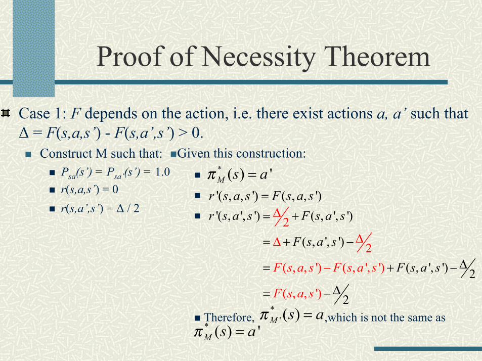
Case 1: F depends on the action, i.e. there exist actions a, a’ such that Δ = F(s,a,s’) - F(s,a’,s’) > 0.
Construct M such that:Psa(s’) = Psa’(s’) = 1.0r(s,a,s’) = 0r(s,a’,s’) = Δ / 2
Given this construction:
Therefore, ,which is not the same as
* ( ) 'M s aπ ='( , , ') ( , , ')r s a s F s a s='( , ', ') ( , ', ')
(2
2( , , ') ( , ', '
, ', ')
( , ', ') 2
2
)
( , , ')
F s
r s a s F s a s
F s a s
F sa s F s a s
F s a s
a s
= +
= + −
∆= +
∆
=
∆∆
− −
∆−*
' ( )M s aπ =* ( ) 'M s aπ =
Proof of Necessity Theorem, cont
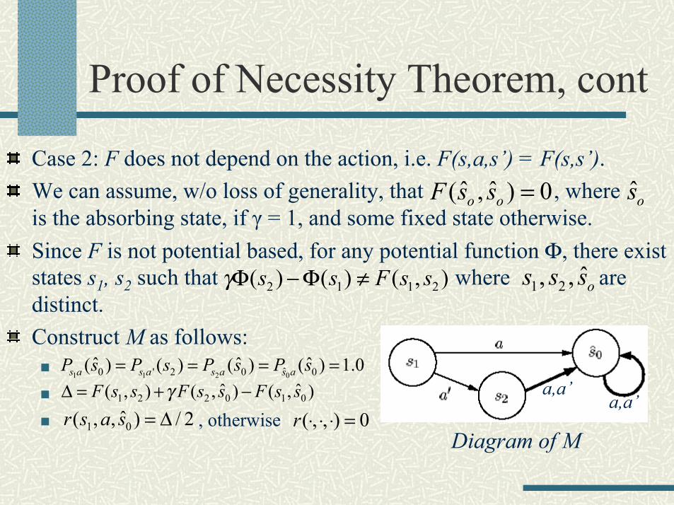
Case 2: F does not depend on the action, i.e. F(s,a,s’) = F(s,s’). We can assume, w/o loss of generality, that , where is the absorbing state, if γ = 1, and some fixed state otherwise.Since F is not potential based, for any potential function Φ, there exist states s1, s2 such that where are distinct.Construct M as follows:
, otherwise
ˆ ˆ( , ) 0o oF s s = ˆos
2 1 1 2( ) ( ) ( , )s s F s sγΦ − Φ ≠ 1 2 ˆ, , os s s
1 1 2 0ˆ0 ' 2 0 0ˆ ˆ ˆ( ) ( ) ( ) ( ) 1.0s a s a s a s aP s P s P s P s= = = =
1 2 2 0 1 0ˆ ˆ( , ) ( , ) ( , )F s s F s s F s sγ∆ = + −
1 0ˆ( , , ) / 2r s a s = ∆ ( , , ) 0r ⋅ ⋅ ⋅ =
a,a’a,a’
Diagram of M

Proof of Necessity Theorem, cont
Therefore, , which is not the same as
a,a’a,a’
1 2 2 0 1
* *1 0
* *1 2
*0
*' 1 1 0
1 0
1 0
1 2 2 0
* *' 1 1 2 '
0
0
2
2
ˆ( , ) ( )2 2( , ') 0 ( )
ˆ0 *0 ( ) 0
ˆ( , ) ( , )
ˆ( , )
ˆ( , ) 2ˆ( , ) ( , ) .2
ˆ( , ')
ˆ ˆ( , ) ( , ) ( ,
,
)
0 ( ) (
M M
M M
M
M
M M
F s s F s s F
Q s a V s
Q s a V sV s
Q s a F s s
F s s
F s s
F s s F s s
Q s a F s s V s
s s
γ
γ
γ
γ
γ
γ
∆ ∆= + =
= +
= + + =
= +
= + −
∆= +
∆
∆
−
∆= + −
=
+
+ +
∆
−
1 2 2 0ˆ) ( , ) ( , )F s s F s sγ= +
Diagram of M
* ( )M s aπ = *' ( ) 'M s aπ =

Choosing a potential function
If then This form makes learning easy because the recursion in the Q-equations has been removed:
Without knowing the actual value of we can use our knowledge about the domain to estimate .
*( ) ( )Ms V sΦ = * * * *' ( ) 0M M M MV V s V V= − Φ = − =
( ) ( )
( )[ ]
* *
'
'
, ' ( , , ') ( ')
' ( , , ') 0
M sa Ms
sas
Q s a P s r s a s V s
P s r s a s
γ = +
= +
∑∑
* ( , )MV s a
* ( , )MV s a

Experiments: Domain 1
Grid-world domain:Domain 1:
-1 reinforcement per stepActions: four directions
Travel 1 step in the intended direction 80%, random direction 20%.
Estimate the expected number of steps to get to the goal from state s as:
A shaping function that is far from the estimate of
G
Sstart
goal
0 ( ) ( 1) ( , ) / 0.8s MANHATTAN s GΦ = − ⋅* ( , ) :MV s a
12 0( ) ( )s sΦ = Φ

Results in Domain 1
Steps taken to reach goal after x iterations of learning in Domain 1
No shaping1
2 0( ) ( )s sΦ = Φ0( ) ( )s sΦ = Φ

Results with 50x50 Grid
Steps taken to reach goal after x iterations of learning in Domain 1
No shaping
12 0( ) ( )s sΦ = Φ
0( ) ( )s sΦ = Φ

Experiments: Domain 2
Domain 2: Must start at S and travel from 1 to 4 in
sequence, then to the goal, G = 5.Actions, rewards are the same as in
Domain 1. Task is completed after the agent has
traveled from 1 to 5 in sequence.If t is the number of time steps to
reach G from S, estimate the numberof steps to go after reaching the nth subgoal as:
0 ( ) ((5 0.5) / 5)s n tΦ = − − −
(5 – n) subgoals to go About halfway between goals n and n+1
5 total goals

is a more precise estimate of the remaining time to goal
Results in Domain 2
Steps taken to reach goal after x iterations of learning in Domain 2
No shaping
0( ) ( )s sΦ = Φˆ( ) ( )Ms V sΦ =
ˆ ( )MV s

Conclusions
Potential-based shaping functions are policy invariant, and are the necessary form to ensure policy invariance. Policy invariance is desired to prevent misleading shaping.
One could also try shaping functions inspired by potential-based shaping functions.Example: The discount factor, γ, is set to be less than 1, not because rewards decrease with time, but to improve convergence. Using an undiscounted shaping function may work.
Potential-based function:Potential-inspired function:
( , , ') ( ') ( )F s a s s sγ= Φ − Φ( , , ') ( ') ( )F s a s s s= Φ − Φ

Conclusions
Following from the robustness argument (near-optimal policies are preserved by potential-based shaping functions), potential-based shaping functions can be used to choose from a class of policies.
Choosing from a class of policies is useful for “parametric” RL,where the policy template is fixed.
This is computationally simpler, more compact, and requires less training.This can also be useful to express knowledge about the domain.
Potential-based shaping functions also generalize to Semi-Markov Decision Processes. “Advantage learning” and “λ-policy iteration” may be used to optimize the potential function used in reward shaping.