Intraday Trading Invariance in the Grain Futures Markets

by

Zhiguang (Gerald) Wang

Suggested citation format:

Wang, Z. 2019. “Intraday Trading Invariance in the Grain Futures Markets.” Proceedings of the NCCC-134 Conference on Applied Commodity Price Analysis, Forecasting, and Market Risk Management. Minneapolis, MN. [http://www.farmdoc.illinois.edu/nccc134].

Intraday Trading Invariance in the Grain Futures Markets

Zhiguang (Gerald) Wang

Paper presented at the NCCC-134 Conference on Applied Commodity Price Analysis,

Forecasting, and Market Risk Management

Minneapolis, Minnesota, April 15-16, 2019

Copyright 2019 by Zhiguang Wang. All rights reserved. Readers may make verbatim

copies of this document for non-commercial purposes by any means, provided that this

copyright notice appears on all such copies.

Wang is an associate professor in the Ness School of Management and of Economics at South

Dakota State University. Wang can be reached at Zhiguang.Wang@sdstate.edu or 605-688-4861.

Intraday Trading Invariance in the Grain FuturesMarkets

Abstract

We test the microstructure invariance proposed by Kyle and Obizhaeva (2016) in thegrain markets. Using the CME’s intraday best-bid-offer data from 2008 to 2015, wefind support for both trade size invariance and trading cost invariance at 1-minute,5-minute, and 10-minute, although not in its original form. After rescaling the tradingactivity by spread cost per Benzaquen et al (2016), we find strong evidence for bothhypotheses of invariance. The findings help understand the trading dynamics of graincommodities from both trading and regulatory perspectives. Specifically, we can derivethe number of trades, trading cost, and illiquidity measure based on observable metrics,such as price, volume and historical volatility. These imputed measures can be furtherused to identify the systematic risks resulting from speculative transactions.

Keywords: Trading Invariance, Grain Futures, Market Microstructure

1 Introduction

It is common knowledge that trading activities, such as trading volume and the numberof trades, are positively related to return volatility. But the exact functional relationshipamong them is not known until Kyle and Obizhaeva’s (2016) microstructure invariance hy-pothesis. They assert through dimension analysis that risk transfer and transaction costsare identical in dollar terms across all assets. A testable hypothesis is that the arrival rateof bets is proportional to the 2/3 power of the risk transfer, i.e. product of expected dollarvolume and return volatility. Their original empirical study validated the hypothesis usinga proprietary portfolio transition dataset on stocks at the daily interval. We propose totest the trading invariance using a public dataset on agricultural commodities, namely corn,soybeans and wheat futures, at the intraday interval.

Understanding endogenous trading dynamics, such as bet sizing, bet arrival rate (numberof bets per day), return volatility and liquidity (Kyle and Obizhaeva (2019)), is crucial tomarket participants as large orders and order splitting become an important aspect of thecurrent electronic market. According to Haynes and Roberts (2015), automated tradingwas involved in 68.7%, 57.7% and 64.4% of corn, soybeans and wheat futures trading. Theintroduction of Globex electronic trading platform for grain futures in 2006 accelerated thefinancialization of agricultural commodities and facilitated large traders’ participation by re-ducing their market impact and trading cost. Irwin and Sanders (2012) reported that openinterests held by large/institutional traders accounted for about 90% in grain futures.

Kyle and Obizhaeva’s microstructure invariance hypothesis provides a powerful frameworkfor connecting such economic variables as trading volume, return volatility, number of trans-actions, and trade size. To the best of our knowledge, there has not been empirical testof intraday trading invariance for grain futures. The previous empirical research has been

1

focused on stock portfolio transition by Kyle and Obizhaeva (2016), on intraday E-mini SPXfutures from 2008 to 2011 by Andersen et al. (2016), and on 12 financial and commodityfutures from 2012 to 2014 by Benzaquen et al. (2016). The first two studies confirmed thetrading invariance within a single market, while the last one found that trading invariancedid not hold true in this original form across different markets. Neither of the last two stud-ies examined the invariance of the trading cost, as they focused only on the number of trades.

We aim to fill the gap by first testing the intraday trading size invariance across the threesimilar yet different electronic grain futures markets. We hypothesize, as with Benzaquenet al. (2016), that there is a need to modify the invariance form to accommodate the dif-ference across the three commodities. We further contribute to the literature by testing theinvariance of trading cost and by examining both trading invariances at different intradayintervals and over different sample periods.

We use a simple linear regression to test the invariances of trade size and trading cost, alongthe lines of Kyle and Obizhaeva (2016). We regress the number of trades and the relativebid-ask spread on trading activity (a multiplication of price, volume and volatility), as op-posed to variance per transaction vs. the average number of trades. We consider both thetrading activity in its original form as in Kyle and Obizhaeva (2016) and the modified formas in Benzaquen et al. (2016).

We will employ the intraday BBO (Best Bid Offer) data from 2008 to 2015 obtained fromthe CME Group. We aggregate the second-by-second data to 1-minute, 5-minute and 10-minute interval. we find support for both trade size invariance and trading cost invarianceat 1-minute, 5-minute, and 10-minute, although not in its original form. After rescalingthe trading activity by spread cost per Benzaquen et al (2016), we find strong evidence forboth hypotheses of invariance. The finding helps understand the trading dynamics of graincommodities from both trading and regulatory perspectives. Specifically, we can derive thenumber of trades, trading cost, and illiquidity measure based on observable metrics, suchas price, volume and historical volatility. These imputed measures can be further used toidentify the systematic risks resulting from speculative transactions.

The rest of the paper is organized as follows. We first describe the microstructure invariancetheory by Kyle and Obizhaeva (2016) in Section 2. We develop three hypotheses related tointraday market microstructure invariance in Section 3. We report the data and empiricalresults for the hypothesis tests in Section 4, and conclude in Section 5.

2 Market Microstructure Invariance

There are two approaches to develop market microstructure invariance: meta-model ap-proach (Kyle and Obizhaeva (2016)) and dimensional analysis (Kyle and Obizhaeva (2017)).Both approaches produce similar results, although the latter makes less assumptions aboutmicroeconomic foundations in a theoretical model. We reproduce Kyle and Obizhaeva’s(2016)) basic results here using the following notations, with dimensions expressed in the

2

bracket. The easy-to-observe variables include:

Price = P [dollars/unit]

Trading V olume = V [units/day]

Returns V olatility = σ [day1/2]

and the following hard-to-measure variables:

Fundamental V alue = F [dollars/unit]

Bet Size = Q [units]

Bet Number or V elocity = γ [/day]

Price Change/Bet = 4P [dollars/unit]

Price Impact = λ [dollars/unit2]

Price Error =

√var(log

F

P) [dimensionless]

Price Resiliency = ρ [dimensionless]

Assuming a power function for price impact and transaction cost (denoted C) invariance, ameta-model can be written as follows:

4P = λQβ (1)

V = γE[|Q|] (2)

σ2 = γE[(4PP

)2] (3)

E[(4P )2] = λ2E[|Q|2β] (4)

C = λE[|Q|1+β] (5)

m =E[|Q|]

√E[|Q|2β]

E[|Q|1+β](6)

mβ =(E[|Q|])1+β

E[|Q|1+β](7)

where the last three variables are invariant across markets, therefore considered constant.The solution to key hard-to-observe variables, illiquidity 1/L, expected bet value E[|PQ|] ,number of bets γ, price impact in percentage 4P

P, and scaled bet value Z can be expressed

3

respectively as follows:

1

L=

C

E[|PQ|]=( σ2C

m2PV

)1/3(8)

Z =|PQ|

E[|PQ|](9)

E[|PQ|] = C · L (10)

γ =1

m2σ2L2 (11)

4PP

=1

Lmβ|

Q

E[|Q|]|β (12)

where L and Z are dimensionless.

In order to solve the hard-to-observe variables, we first invoke the market microstructureinvariance, hypothesizing that (1) the dollar distribution of the gains or losses from bets(dollar risk transfer) is the same across all markets when measured in units of business time:

IB = P ·Q · σ

γ1/2(13)

and (2) the dollar cost of executing bets is the same function of their risk transfers IB acrossall markets: CB(IB), where the subscript B stands for bet. So is the average (or uncondi-tional mean) cost of executing bets CB = E[CB(IB)].

We then define trading activity WB as dollar volume per bet adjusted for volatility. It is ameasure of gross risk transfer:

WB = σ · P · V = σ · P · E[|Q|] · γ

Based on the two measures of risk transfer (IB and WB), we can express number of bets γ,relative bet size Q

V, and percentage cost of executing a bet C(Q) as

γ = W2/3B · {E[|IB|]}−2/3 (14)

Q

V= W

−2/3B · {E[|IB|]}−1/3 · IB (15)

E[|Q|] = W1/3B · 1

Pσ· {E[|IB|]}2/3 (16)

C(Q) =CB(IB)

P |Q|=

1

L· f(IB) (17)

where f(IB) = CB(IB)IB

E[IB ]E[CB(IB)]

is invariance average price impact function. Equation (14)will become a basis of our test for invariance of risk transfer.

For different average impact functions f(I), the cost function will take different forms, buthas two components: bid-ask spread cost and market impact cost. For a linear model the

4

average impaction function and the cost function are derived as

f(I) = [E|I|]−1/3κ+ [E|I|]−2/3λ · |I|

C(Q) = σ[κW−1/3 + λE[W ]1/3

|Q|E[V ]

]For a square root model, the average impaction function and the cost function are derivedas

f(I) = [E|I|]−1/3κ+ [E|I|]−1/2λ · |I|1/2

C(Q) = σ[κW−1/3 + λ

√|Q|E[V ]

]In either case, the bid-ask spread cost scaled by volatility σ is proportional to trading activityW−1/3. If the spread cost is measured in percentage, we have the linear relationship betweenspread cost and trading activity:

BASP

σ∝ W−1/3 (18)

Equation (18) will become of our test for invariance of trading cost.

3 Hypothesis Development

The invariance that underlies Kyle and Obizhaeva (2016) is based on bets, not necessarily tointraday trades. As with Andersen et al. (2016), we can obtain intraday trading invarianceby assuming that the average number of transactions per bet is invariant across assets andtime, i.e. the proportional relationship between number of trades N and number of bets γ:N ∼ γ. We can restate Equation 13 for any intraday time interval t.

It = Pt ·Qt ·σt

γ1/2t

(19)

where the definition of all variables remain the same except that they are defined for thenon-overlapping intraday interval, as opposed to daily interval. As such, we hypothesize thatsuch invariance can broadly hold true to trades.

Hypothesis 1: number of trades N , adjusted for differences in trading activityW , are the same across different commodities.

Based on Equation 15, the invariance of bet size lies in ln(|Q|V·[W]2/3)

or equivalently

ln(N ·

[W]2/3)

per Equation 14. By substituting order size X for bet size Q, we can cast

the trading invariance in the following testable regression format:

5

ln[VX

]= −ln[q] + α1 · ln

[W]

+ ε (20)

ln[N]

= const+ α1 · ln[W]

+ ε (21)

where V is trading volume, X is order size, N is the number of trades (a proxy for thenumber of bet γ in Equation (11)), W is trading activity, q is median size of liquidity trade.The second equation is a simplification of the first equation, where the intercept const is ameasure of bet number or risk transfer for a benchmark asset. The null hypothesis is thatα1 = 2/3.

Hypothesis 2: trading cost as measured by quoted relative bid-ask spread, scaledby volatility, does not vary across difference commodities.

Quoted bid-ask spread in dollars S corresponds to the first component of the cost functionC(Q). The invariance hypothesis from Equation 18 implies the relative bid-ask spread scaledby volatility is proportional to trading activity.

ln[BAS

P ∗ σ] = const+ α2 · ln

[W]

+ ε (22)

where BAS is the quoted bid-ask spread, P is trade price, σ is volatility and W is tradingactivity. The intercept const can be interpreted as trading cost for a benchmark asset. Thenull hypothesis is that α2 = −1/3.

4 Data and Results

4.1 Data

The Trade and Quote data for corn, soybeans, and wheat futures are obtained from Weobtain from the CME (Chicago Mercantile Exchange) Group. The CME intraday data isstamped to second. The time period ranges from January 2008 to May 2015. We use onlythe nearby futures contract for our empirical analysis.

As noted by Andersen et al. (2016), the CME group reports all contracts traded at aparticular price as a single transaction, therefore treating the incoming order as a whole.Table I presents summary statistics for the three commodities at 1-minute interval. Fivevariables are reported in the table: last trade price, number of trades, trading volume, num-ber of contracts per trade, bid-ask spread in ticks. As with Andersen et al. (2016), weaverage these variables at the 1-minute interval and then across all sample days in order tominimize the sample noise. Average prices for corn, soybeans and wheat during the sampleperiod are $5.18/bushel, $12.31/bushel, and $6.56/bushel, respectively. It is clear from TableI that all variables, with the exception of price, show varying degree of skewness and kurtosis.

6

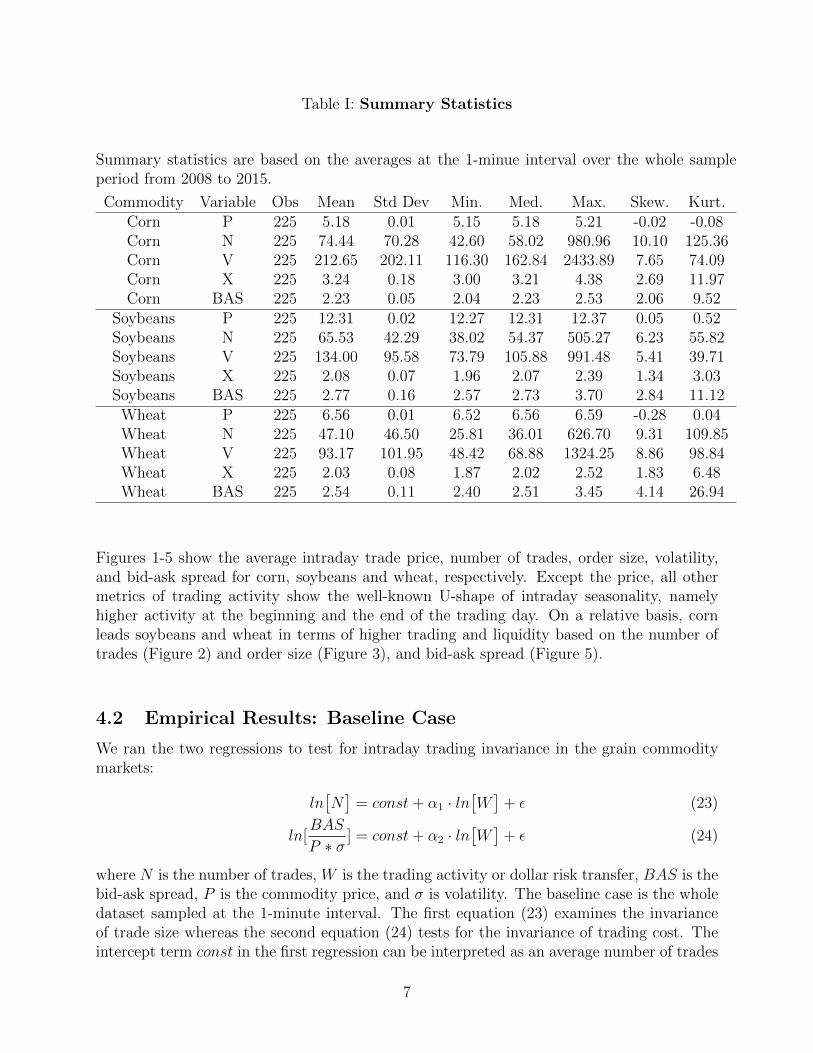
Table I: Summary Statistics

Summary statistics are based on the averages at the 1-minue interval over the whole sampleperiod from 2008 to 2015.

Commodity Variable Obs Mean Std Dev Min. Med. Max. Skew. Kurt.Corn P 225 5.18 0.01 5.15 5.18 5.21 -0.02 -0.08Corn N 225 74.44 70.28 42.60 58.02 980.96 10.10 125.36Corn V 225 212.65 202.11 116.30 162.84 2433.89 7.65 74.09Corn X 225 3.24 0.18 3.00 3.21 4.38 2.69 11.97Corn BAS 225 2.23 0.05 2.04 2.23 2.53 2.06 9.52

Soybeans P 225 12.31 0.02 12.27 12.31 12.37 0.05 0.52Soybeans N 225 65.53 42.29 38.02 54.37 505.27 6.23 55.82Soybeans V 225 134.00 95.58 73.79 105.88 991.48 5.41 39.71Soybeans X 225 2.08 0.07 1.96 2.07 2.39 1.34 3.03Soybeans BAS 225 2.77 0.16 2.57 2.73 3.70 2.84 11.12

Wheat P 225 6.56 0.01 6.52 6.56 6.59 -0.28 0.04Wheat N 225 47.10 46.50 25.81 36.01 626.70 9.31 109.85Wheat V 225 93.17 101.95 48.42 68.88 1324.25 8.86 98.84Wheat X 225 2.03 0.08 1.87 2.02 2.52 1.83 6.48Wheat BAS 225 2.54 0.11 2.40 2.51 3.45 4.14 26.94

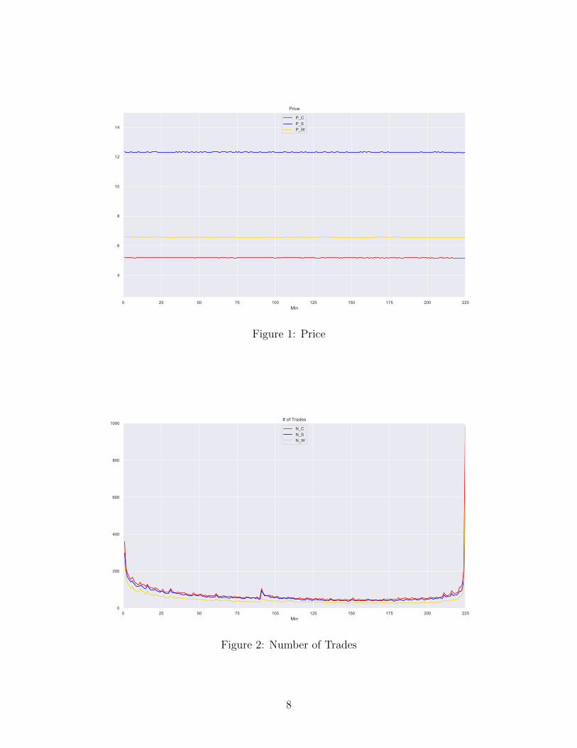
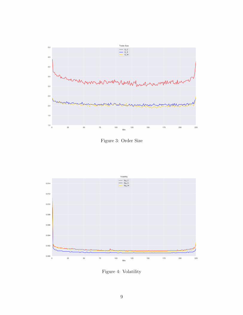
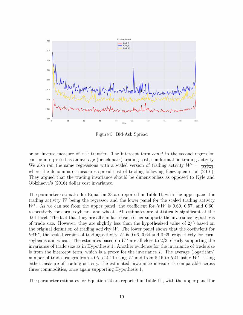
Figures 1-5 show the average intraday trade price, number of trades, order size, volatility,and bid-ask spread for corn, soybeans and wheat, respectively. Except the price, all othermetrics of trading activity show the well-known U-shape of intraday seasonality, namelyhigher activity at the beginning and the end of the trading day. On a relative basis, cornleads soybeans and wheat in terms of higher trading and liquidity based on the number oftrades (Figure 2) and order size (Figure 3), and bid-ask spread (Figure 5).

4.2 Empirical Results: Baseline Case

We ran the two regressions to test for intraday trading invariance in the grain commoditymarkets:

ln[N]

= const+ α1 · ln[W]

+ ε (23)

ln[BAS

P ∗ σ] = const+ α2 · ln

[W]

+ ε (24)

where N is the number of trades, W is the trading activity or dollar risk transfer, BAS is thebid-ask spread, P is the commodity price, and σ is volatility. The baseline case is the wholedataset sampled at the 1-minute interval. The first equation (23) examines the invarianceof trade size whereas the second equation (24) tests for the invariance of trading cost. Theintercept term const in the first regression can be interpreted as an average number of trades

7

0 25 50 75 100 125 150 175 200 225Min

4

6

8

10

12

14

Price

P_CP_SP_W

Figure 1: Price

0 25 50 75 100 125 150 175 200 225Min

0

200

400

600

800

1000# of Trades

N_CN_SN_W

Figure 2: Number of Trades

8

0 25 50 75 100 125 150 175 200 225Min

1.0

1.5

2.0

2.5

3.0

3.5

4.0

4.5

5.0Trade Size

Q_CQ_SQ_W

Figure 3: Order Size

0 25 50 75 100 125 150 175 200 225Min

0.000

0.002

0.004

0.006

0.008

0.010

0.012

0.014

Volatility

Sig_CSig_SSig_W

Figure 4: Volatility

9

0 25 50 75 100 125 150 175 200 225Min

2.00

2.25

2.50

2.75

3.00

3.25

3.50

3.75

4.00Bid-Ask Spread

BAS_CBAS_SBAS_W

Figure 5: Bid-Ask Spread

or an inverse measure of risk transfer. The intercept term const in the second regressioncan be interpreted as an average (benchmark) trading cost, conditional on trading activity.We also ran the same regressions with a scaled version of trading activity W ∗ = W

BAS∗Q ,

where the denominator measures spread cost of trading following Benzaquen et al (2016).They argued that the trading invariance should be dimensionless as opposed to Kyle andObizhaeva’s (2016) dollar cost invariance.

The parameter estimates for Equation 23 are reported in Table II, with the upper panel fortrading activity W being the regressor and the lower panel for the scaled trading activityW ∗. As we can see from the upper panel, the coefficient for lnW is 0.60, 0.57, and 0.60,respectively for corn, soybeans and wheat. All estimates are statistically significant at the0.01 level. The fact that they are all similar to each other supports the invariance hypothesisof trade size. However, they are slightly less than the hypothesized value of 2/3 based onthe original definition of trading activity W . The lower panel shows that the coefficient forlnW ∗, the scaled version of trading activity W is 0.66, 0.64 and 0.66, respectively for corn,soybeans and wheat. The estimates based on W ∗ are all close to 2/3, clearly supporting theinvariance of trade size as in Hypothesis 1. Another evidence for the invariance of trade sizeis from the intercept term, which is a proxy for the invariance I. The average (logarithm)number of trades ranges from 4.05 to 4.11 using W and from 5.16 to 5.41 using W ∗. Usingeither measure of trading activity, the estimated invariance measure is comparable acrossthree commodities, once again supporting Hypothesis 1.

The parameter estimates for Equation 24 are reported in Table III, with the upper panel for

10

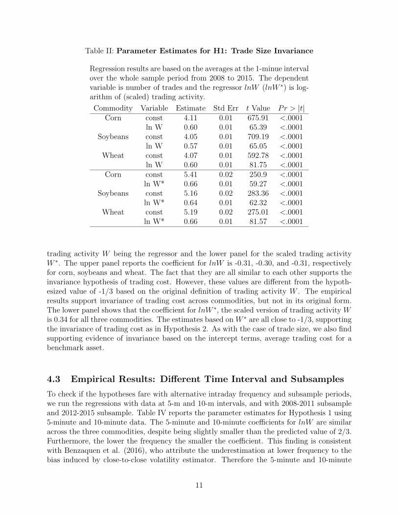
Table II: Parameter Estimates for H1: Trade Size Invariance

Regression results are based on the averages at the 1-minue intervalover the whole sample period from 2008 to 2015. The dependentvariable is number of trades and the regressor lnW (lnW ∗) is log-arithm of (scaled) trading activity.

Commodity Variable Estimate Std Err t Value Pr > |t|Corn const 4.11 0.01 675.91 <.0001

ln W 0.60 0.01 65.39 <.0001Soybeans const 4.05 0.01 709.19 <.0001

ln W 0.57 0.01 65.05 <.0001Wheat const 4.07 0.01 592.78 <.0001

ln W 0.60 0.01 81.75 <.0001Corn const 5.41 0.02 250.9 <.0001

ln W* 0.66 0.01 59.27 <.0001Soybeans const 5.16 0.02 283.36 <.0001

ln W* 0.64 0.01 62.32 <.0001Wheat const 5.19 0.02 275.01 <.0001

ln W* 0.66 0.01 81.57 <.0001

trading activity W being the regressor and the lower panel for the scaled trading activityW ∗. The upper panel reports the coefficient for lnW is -0.31, -0.30, and -0.31, respectivelyfor corn, soybeans and wheat. The fact that they are all similar to each other supports theinvariance hypothesis of trading cost. However, these values are different from the hypoth-esized value of -1/3 based on the original definition of trading activity W . The empiricalresults support invariance of trading cost across commodities, but not in its original form.The lower panel shows that the coefficient for lnW ∗, the scaled version of trading activity Wis 0.34 for all three commodities. The estimates based on W ∗ are all close to -1/3, supportingthe invariance of trading cost as in Hypothesis 2. As with the case of trade size, we also findsupporting evidence of invariance based on the intercept terms, average trading cost for abenchmark asset.

4.3 Empirical Results: Different Time Interval and Subsamples

To check if the hypotheses fare with alternative intraday frequency and subsample periods,we run the regressions with data at 5-m and 10-m intervals, and with 2008-2011 subsampleand 2012-2015 subsample. Table IV reports the parameter estimates for Hypothesis 1 using5-minute and 10-minute data. The 5-minute and 10-minute coefficients for lnW are similaracross the three commodities, despite being slightly smaller than the predicted value of 2/3.Furthermore, the lower the frequency the smaller the coefficient. This finding is consistentwith Benzaquen et al. (2016), who attribute the underestimation at lower frequency to thebias induced by close-to-close volatility estimator. Therefore the 5-minute and 10-minute

11

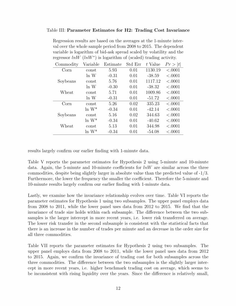
Table III: Parameter Estimates for H2: Trading Cost Invariance

Regression results are based on the averages at the 1-minute inter-val over the whole sample period from 2008 to 2015. The dependentvariable is logarithm of bid-ask spread scaled by volatility and theregressor lnW (lnW ∗) is logarithm of (scaled) trading activity.

Commodity Variable Estimate Std Err t Value Pr > |t|Corn const 5.93 0.01 1130.19 <.0001

ln W -0.31 0.01 -38.59 <.0001Soybeans const 5.76 0.01 1117.12 <.0001

ln W -0.30 0.01 -38.32 <.0001Wheat const 5.71 0.01 1009.86 <.0001

ln W -0.31 0.01 -51.72 <.0001Corn const 5.26 0.02 335.23 <.0001

ln W* -0.34 0.01 -42.14 <.0001Soybeans const 5.16 0.02 344.63 <.0001

ln W* -0.34 0.01 -40.62 <.0001Wheat const 5.13 0.01 344.98 <.0001

ln W* -0.34 0.01 -54.08 <.0001

results largely confirm our earlier finding with 1-minute data.

Table V reports the parameter estimates for Hypothesis 2 using 5-minute and 10-minutedata. Again, the 5-minute and 10-minute coefficients for lnW are similar across the threecommodities, despite being slightly larger in absolute value than the predicted value of -1/3.Furthermore, the lower the frequency the smaller the coefficient. Therefore the 5-minute and10-minute results largely confirm our earlier finding with 1-minute data.

Lastly, we examine how the invariance relationship evolves over time. Table VI reports theparameter estimates for Hypothesis 1 using two subsamples. The upper panel employs datafrom 2008 to 2011, while the lower panel uses data from 2012 to 2015. We find that theinvariance of trade size holds within each subsample. The difference between the two sub-samples is the larger intercept in more recent years, i.e. lower risk transferred on average.The lower risk transfer in the second subsample is consistent with the statistical facts thatthere is an increase in the number of trades per minute and an decrease in the order size forall three commodities.

Table VII reports the parameter estimates for Hypothesis 2 using two subsamples. Theupper panel employs data from 2008 to 2011, while the lower panel uses data from 2012to 2015. Again, we confirm the invariance of trading cost for both subsamples across thethree commodities. The difference between the two subsamples is the slightly larger inter-cept in more recent years, i.e. higher benchmark trading cost on average, which seems tobe inconsistent with rising liquidity over the years. Since the difference is relatively small,

12

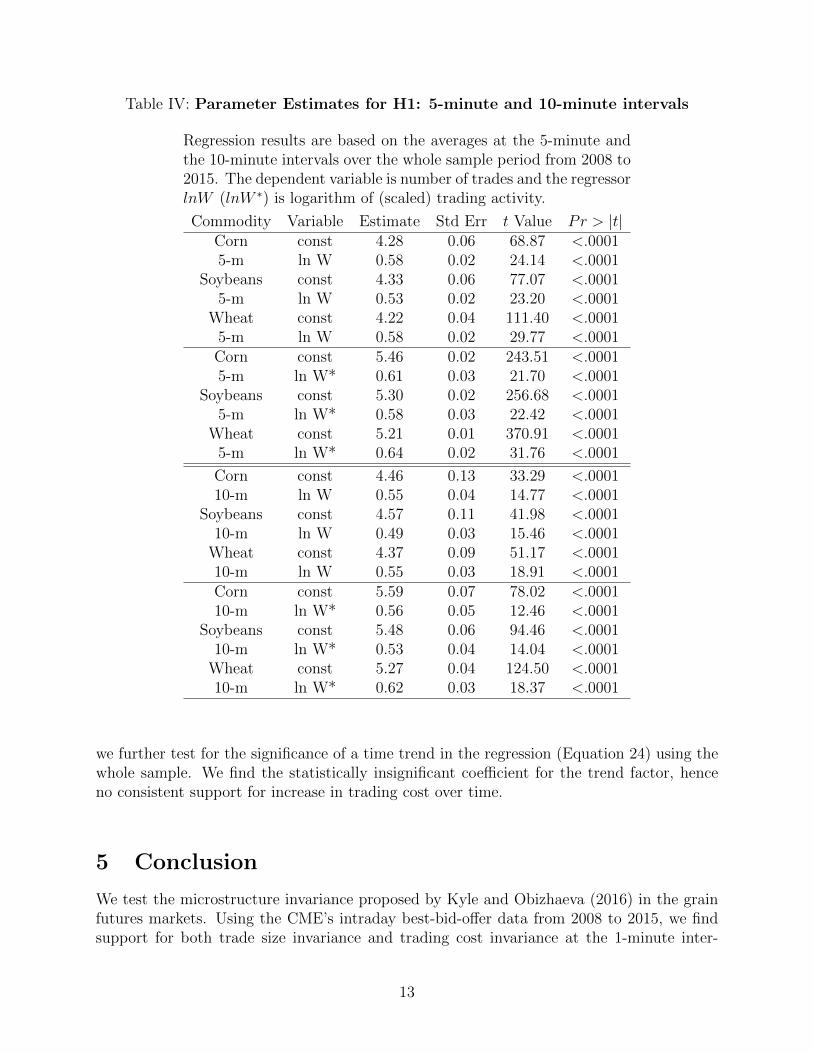
Table IV: Parameter Estimates for H1: 5-minute and 10-minute intervals

Regression results are based on the averages at the 5-minute andthe 10-minute intervals over the whole sample period from 2008 to2015. The dependent variable is number of trades and the regressorlnW (lnW ∗) is logarithm of (scaled) trading activity.

Commodity Variable Estimate Std Err t Value Pr > |t|Corn const 4.28 0.06 68.87 <.00015-m ln W 0.58 0.02 24.14 <.0001

Soybeans const 4.33 0.06 77.07 <.00015-m ln W 0.53 0.02 23.20 <.0001

Wheat const 4.22 0.04 111.40 <.00015-m ln W 0.58 0.02 29.77 <.0001Corn const 5.46 0.02 243.51 <.00015-m ln W* 0.61 0.03 21.70 <.0001

Soybeans const 5.30 0.02 256.68 <.00015-m ln W* 0.58 0.03 22.42 <.0001

Wheat const 5.21 0.01 370.91 <.00015-m ln W* 0.64 0.02 31.76 <.0001

Corn const 4.46 0.13 33.29 <.000110-m ln W 0.55 0.04 14.77 <.0001

Soybeans const 4.57 0.11 41.98 <.000110-m ln W 0.49 0.03 15.46 <.0001

Wheat const 4.37 0.09 51.17 <.000110-m ln W 0.55 0.03 18.91 <.0001Corn const 5.59 0.07 78.02 <.000110-m ln W* 0.56 0.05 12.46 <.0001

Soybeans const 5.48 0.06 94.46 <.000110-m ln W* 0.53 0.04 14.04 <.0001

Wheat const 5.27 0.04 124.50 <.000110-m ln W* 0.62 0.03 18.37 <.0001

we further test for the significance of a time trend in the regression (Equation 24) using thewhole sample. We find the statistically insignificant coefficient for the trend factor, henceno consistent support for increase in trading cost over time.

5 Conclusion

We test the microstructure invariance proposed by Kyle and Obizhaeva (2016) in the grainfutures markets. Using the CME’s intraday best-bid-offer data from 2008 to 2015, we findsupport for both trade size invariance and trading cost invariance at the 1-minute inter-

13

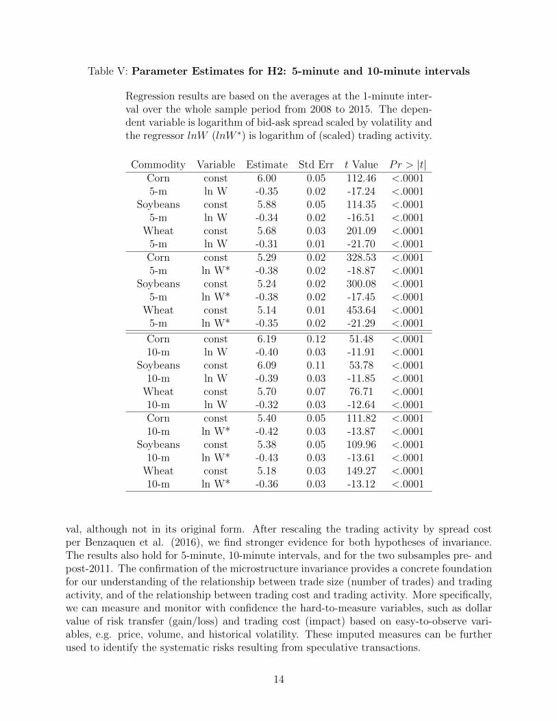
Table V: Parameter Estimates for H2: 5-minute and 10-minute intervals

Regression results are based on the averages at the 1-minute inter-val over the whole sample period from 2008 to 2015. The depen-dent variable is logarithm of bid-ask spread scaled by volatility andthe regressor lnW (lnW ∗) is logarithm of (scaled) trading activity.

Commodity Variable Estimate Std Err t Value Pr > |t|Corn const 6.00 0.05 112.46 <.00015-m ln W -0.35 0.02 -17.24 <.0001

Soybeans const 5.88 0.05 114.35 <.00015-m ln W -0.34 0.02 -16.51 <.0001

Wheat const 5.68 0.03 201.09 <.00015-m ln W -0.31 0.01 -21.70 <.0001Corn const 5.29 0.02 328.53 <.00015-m ln W* -0.38 0.02 -18.87 <.0001

Soybeans const 5.24 0.02 300.08 <.00015-m ln W* -0.38 0.02 -17.45 <.0001

Wheat const 5.14 0.01 453.64 <.00015-m ln W* -0.35 0.02 -21.29 <.0001

Corn const 6.19 0.12 51.48 <.000110-m ln W -0.40 0.03 -11.91 <.0001

Soybeans const 6.09 0.11 53.78 <.000110-m ln W -0.39 0.03 -11.85 <.0001

Wheat const 5.70 0.07 76.71 <.000110-m ln W -0.32 0.03 -12.64 <.0001Corn const 5.40 0.05 111.82 <.000110-m ln W* -0.42 0.03 -13.87 <.0001

Soybeans const 5.38 0.05 109.96 <.000110-m ln W* -0.43 0.03 -13.61 <.0001

Wheat const 5.18 0.03 149.27 <.000110-m ln W* -0.36 0.03 -13.12 <.0001

val, although not in its original form. After rescaling the trading activity by spread costper Benzaquen et al. (2016), we find stronger evidence for both hypotheses of invariance.The results also hold for 5-minute, 10-minute intervals, and for the two subsamples pre- andpost-2011. The confirmation of the microstructure invariance provides a concrete foundationfor our understanding of the relationship between trade size (number of trades) and tradingactivity, and of the relationship between trading cost and trading activity. More specifically,we can measure and monitor with confidence the hard-to-measure variables, such as dollarvalue of risk transfer (gain/loss) and trading cost (impact) based on easy-to-observe vari-ables, e.g. price, volume, and historical volatility. These imputed measures can be furtherused to identify the systematic risks resulting from speculative transactions.

14

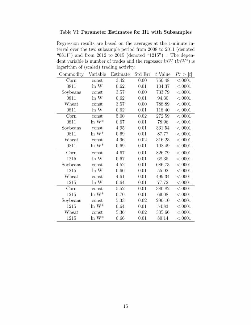
Table VI: Parameter Estimates for H1 with Subsamples

Regression results are based on the averages at the 1-minute in-terval over the two subsample period from 2008 to 2011 (denoted“0811”) and from 2012 to 2015 (denoted “1215”) . The depen-dent variable is number of trades and the regressor lnW (lnW ∗) islogarithm of (scaled) trading activity.

Commodity Variable Estimate Std Err t Value Pr > |t|Corn const 3.42 0.00 750.48 <.00010811 ln W 0.62 0.01 104.37 <.0001

Soybeans const 3.57 0.00 733.79 <.00010811 ln W 0.62 0.01 94.30 <.0001

Wheat const 3.57 0.00 788.89 <.00010811 ln W 0.62 0.01 118.40 <.0001Corn const 5.00 0.02 272.59 <.00010811 ln W* 0.67 0.01 78.96 <.0001

Soybeans const 4.95 0.01 331.54 <.00010811 ln W* 0.69 0.01 87.77 <.0001

Wheat const 4.96 0.02 316.23 <.00010811 ln W* 0.69 0.01 108.49 <.0001

Corn const 4.67 0.01 826.79 <.00011215 ln W 0.67 0.01 68.35 <.0001

Soybeans const 4.52 0.01 686.73 <.00011215 ln W 0.60 0.01 55.92 <.0001

Wheat const 4.61 0.01 499.34 <.00011215 ln W 0.64 0.01 77.72 <.0001Corn const 5.52 0.01 380.82 <.00011215 ln W* 0.70 0.01 69.08 <.0001

Soybeans const 5.33 0.02 290.10 <.00011215 ln W* 0.64 0.01 54.83 <.0001

Wheat const 5.36 0.02 305.66 <.00011215 ln W* 0.66 0.01 80.14 <.0001

15

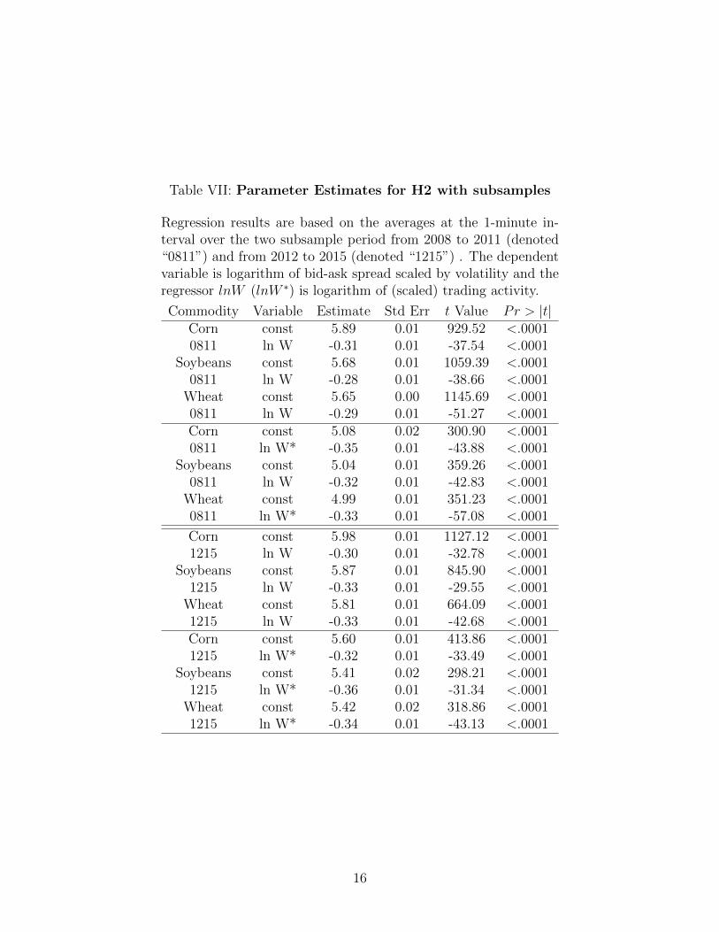
Table VII: Parameter Estimates for H2 with subsamples

Regression results are based on the averages at the 1-minute in-terval over the two subsample period from 2008 to 2011 (denoted“0811”) and from 2012 to 2015 (denoted “1215”) . The dependentvariable is logarithm of bid-ask spread scaled by volatility and theregressor lnW (lnW ∗) is logarithm of (scaled) trading activity.

Commodity Variable Estimate Std Err t Value Pr > |t|Corn const 5.89 0.01 929.52 <.00010811 ln W -0.31 0.01 -37.54 <.0001

Soybeans const 5.68 0.01 1059.39 <.00010811 ln W -0.28 0.01 -38.66 <.0001

Wheat const 5.65 0.00 1145.69 <.00010811 ln W -0.29 0.01 -51.27 <.0001Corn const 5.08 0.02 300.90 <.00010811 ln W* -0.35 0.01 -43.88 <.0001

Soybeans const 5.04 0.01 359.26 <.00010811 ln W -0.32 0.01 -42.83 <.0001

Wheat const 4.99 0.01 351.23 <.00010811 ln W* -0.33 0.01 -57.08 <.0001

Corn const 5.98 0.01 1127.12 <.00011215 ln W -0.30 0.01 -32.78 <.0001

Soybeans const 5.87 0.01 845.90 <.00011215 ln W -0.33 0.01 -29.55 <.0001

Wheat const 5.81 0.01 664.09 <.00011215 ln W -0.33 0.01 -42.68 <.0001Corn const 5.60 0.01 413.86 <.00011215 ln W* -0.32 0.01 -33.49 <.0001

Soybeans const 5.41 0.02 298.21 <.00011215 ln W* -0.36 0.01 -31.34 <.0001

Wheat const 5.42 0.02 318.86 <.00011215 ln W* -0.34 0.01 -43.13 <.0001

16

References

Andersen, T., B. O. K. A. O. A. and T. Tuzun (2016). Intraday trading invariance in thee-mini s&p 500 futures market. Working Paper .

Benzaquen, M., J. Donier, and J.-P. Bouchaud (2016). Unravelling the trading invariancehypothesis. Market Microstructure and Liquidity 02 (03n04), 1650009.

Haynes, R. and J. Roberts (2015). Automated trading in futures markets. Office of ChiefEconomist, CFTC White Paper .

Kyle, A. S. and A. A. Obizhaeva (2016). Market microstructure invariance: Empiricalhypotheses. Econometrica 84 (4), 1345–1404.

Kyle, A. S. and A. A. Obizhaeva (2017). Dimensional analysis, leverage neutrality, andmarket microstructure invariance. Working Paper .

Kyle, A. S. and A. A. Obizhaeva (2019). Market microstructure invariance: A dynamicequilibrium model. Working Paper .

17