8/12/2019 Scale Invariance

http://slidepdf.com/reader/full/scale-invariance 1/9

8/12/2019 Scale Invariance

http://slidepdf.com/reader/full/scale-invariance 2/9

Scale invariance 2

Projective geometry

The idea of scale invariance of a monomial generalizes in higher dimensions to the idea of a homogeneous

polynomial, and more generally to a homogeneous function. Homogeneous functions are the natural denizens of

projective space, and homogeneous polynomials are studied as projective varieties in projective geometry. Projective

geometry is a particularly rich field of mathematics; in its most abstract forms, the geometry of schemes, it has

connections to various topics in string theory.

Fractals

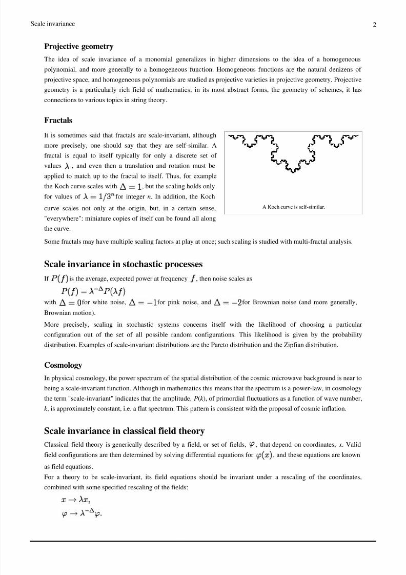
A Koch curve is self-similar.

It is sometimes said that fractals are scale-invariant, although

more precisely, one should say that they are self-similar. A

fractal is equal to itself typically for only a discrete set of

values , and even then a translation and rotation must be

applied to match up to the fractal to itself. Thus, for example

the Koch curve scales with , but the scaling holds only

for values of for integer n. In addition, the Koch

curve scales not only at the origin, but, in a certain sense,

"everywhere": miniature copies of itself can be found all along

the curve.

Some fractals may have multiple scaling factors at play at once; such scaling is studied with multi-fractal analysis.

Scale invariance in stochastic processesIf is the average, expected power at frequency , then noise scales as

with for white noise, for pink noise, and for Brownian noise (and more generally,Brownian motion).

More precisely, scaling in stochastic systems concerns itself with the likelihood of choosing a particular

configuration out of the set of all possible random configurations. This likelihood is given by the probability

distribution. Examples of scale-invariant distributions are the Pareto distribution and the Zipfian distribution.

Cosmology

In physical cosmology, the power spectrum of the spatial distribution of the cosmic microwave background is near to

being a scale-invariant function. Although in mathematics this means that the spectrum is a power-law, in cosmology

the term "scale-invariant" indicates that the amplitude, P (k ), of primordial fluctuations as a function of wave number,

k , is approximately constant, i.e. a flat spectrum. This pattern is consistent with the proposal of cosmic inflation.

Scale invariance in classical field theoryClassical field theory is generically described by a field, or set of fields, , that depend on coordinates, x. Valid

field configurations are then determined by solving differential equations for , and these equations are known

as field equations.

For a theory to be scale-invariant, its field equations should be invariant under a rescaling of the coordinates,

combined with some specified rescaling of the fields:

8/12/2019 Scale Invariance

http://slidepdf.com/reader/full/scale-invariance 3/9

Scale invariance 3

The parameter is known as the scaling dimension of the field, and its value depends on the theory under

consideration. Scale invariance will typically hold provided that no fixed length scale appears in the theory.

Conversely, the presence of a fixed length scale indicates that a theory is not scale-invariant.

A consequence of scale invariance is that given a solution of a scale-invariant field equation, we can automatically

find other solutions by rescaling both the coordinates and the fields appropriately. In technical terms, given a

solution, , one always has other solutions of the form .

Scale invariance of field configurations

For a particular field configuration, , to be scale-invariant, we require that

where is again the scaling dimension of the field.

We note that this condition is rather restrictive. In general, solutions even of scale-invariant field equations will not

be scale-invariant, and in such cases the symmetry is said to be spontaneously broken.

Classical electromagnetismAn example of a scale-invariant classical field theory is electromagnetism with no charges or currents. The fields are

the electric and magnetic fields, and , while their field equations are Maxwell's equations. With

no charges or currents, these field equations take the form of wave equations

where c is the speed of light.

These field equations are invariant under the transformation

Moreover, given solutions of Maxwell's equations, and , we have that and

are also solutions.

Massless scalar field theory

Another example of a scale-invariant classical field theory is the massless scalar field (note that the name scalar is

unrelated to scale invariance). The scalar field, is a function of a set of spatial variables, , and a time

variable, t. We first consider the linear theory. Much like the electromagnetic field equations above, the equation of motion for this theory is also a wave equation

and is invariant under the transformation

The name massless refers to the absence of a term in the field equation. Such a term is often referred to as

a `mass' term, and would break the invariance under the above transformation. In relativistic field theories, a

mass-scale, is physically equivalent to a fixed length scale via

8/12/2019 Scale Invariance

http://slidepdf.com/reader/full/scale-invariance 4/9

Scale invariance 4

and so it should not be surprising that massive scalar field theory is not scale-invariant.

€ 4 theory

The field equations in the examples above are all linear in the fields, which has meant that the scaling dimension,

, has not been so important. However, one usually requires that the scalar field action is dimensionless, and this fixes

the scaling dimension of . In particular,

where D is the combined number of spatial and time dimensions.

Given this scaling dimension for , there are certain nonlinear modifications of massless scalar field theory which

are also scale-invariant. One example is massless ‚ 4 theory for . The field equation is

(Note that the name derives from the form of the Lagrangian, which contains the fourth power of .)

When D=4 (e.g. three spatial dimensions and one time dimension), the scalar field scaling dimension is .

The field equation is then invariant under the transformation

The key point is that the parameter g must be dimensionless, otherwise one introduces a fixed length scale into the

theory. For ‚ 4 theory this is only the case in .

Scale invariance in quantum field theory

The scale-dependence of a quantum field theory (QFT) is characterised by the way its coupling parameters dependon the energy-scale of a given physical process. This energy dependence is described by the renormalization group,

and is encoded in the beta-functions of the theory.

For a QFT to be scale-invariant, its coupling parameters must be independent of the energy-scale, and this is

indicated by the vanishing of the beta-functions of the theory. Such theories are also known as fixed points of the

corresponding renormalization group flow.

Quantum electrodynamics

A simple example of a scale-invariant QFT is the quantized electromagnetic field without charged particles. This

theory actually has no coupling parameters (since photons are massless and non-interacting) and is therefore

scale-invariant, much like the classical theory.

However, in nature the electromagnetic field is coupled to charged particles, such as electrons. The QFT describing

the interactions of photons and charged particles is quantum electrodynamics (QED), and this theory is not

scale-invariant. We can see this from the QED beta-function. This tells us that the electric charge (which is the

coupling parameter in the theory) increases with increasing energy. Therefore, while the quantized electromagnetic

field without charged particles is scale-invariant, QED is not scale-invariant.

8/12/2019 Scale Invariance

http://slidepdf.com/reader/full/scale-invariance 5/9

Scale invariance 5

Massless scalar field theory

Free, massless quantized scalar field theory has no coupling parameters. Therefore, like the classical version, it is

scale-invariant. In the language of the renormalization group, this theory is known as the Gaussian fixed point.

However, even though the classical massless ‚ 4 theory is scale-invariant in , the quantized version is not

scale-invariant. We can see this from the beta-function for the coupling parameter, g.

Even though the quantized massless ‚ 4 is not scale-invariant, there do exist scale-invariant quantized scalar field

theories other than the Gaussian fixed point. One example is the Wilson-Fisher fixed point.

Conformal field theory

Scale-invariant QFTs are almost always invariant under the full conformal symmetry, and the study of such QFTs is

conformal field theory (CFT). Operators in a CFT have a well-defined scaling dimension, analogous to the scaling

dimension, , of a classical field discussed above. However, the scaling dimensions of operators in a CFT typically

differ from those of the fields in the corresponding classical theory. The additional contributions appearing in the

CFT are known as anomalous scaling dimensions.

Scale and conformal anomalies

The ‚ 4 theory example above demonstrates that the coupling parameters of a quantum field theory can be

scale-dependent even if the corresponding classical field theory is scale-invariant (or conformally invariant). If this is

the case, the classical scale (or conformal) invariance is said to be anomalous.

Phase transitionsIn statistical mechanics, as a system undergoes a phase transition, its fluctuations are described by a scale-invariant

statistical field theory. For a system in equilibrium (i.e. time-independent) in D spatial dimensions, the corresponding

statistical field theory is formally similar to a D-dimensional CFT. The scaling dimensions in such problems are

usually referred to as critical exponents, and one can in principle compute these exponents in the appropriate CFT.

The Ising model

An example that links together many of the ideas in this article is the phase transition of the Ising model, a simple

model of ferromagnetic substances. This is a statistical mechanics model which also has a description in terms of

conformal field theory. The system consists of an array of lattice sites, which form a D-dimensional periodic lattice.

Associated with each lattice site is a magnetic moment, or spin, and this spin can take either the value +1 or -1.

(These states are also called up and down, respectively.)

The key point is that the Ising model has a spin-spin interaction, making it energetically favourable for two adjacent

spins to be aligned. On the other hand, thermal fluctuations typically introduce a randomness into the alignment of spins. At some critical temperature, , spontaneous magnetization is said to occur. This means that below the

spin-spin interaction will begin to dominate, and there is some net alignment of spins in one of the two directions.

An example of the kind of physical quantities one would like to calculate at this critical temperature is the correlation

between spins separated by a distance r. This has the generic behaviour:

for some particular value of , which is an example of a critical exponent.

8/12/2019 Scale Invariance

http://slidepdf.com/reader/full/scale-invariance 6/9

Scale invariance 6

CFT description

The fluctuations at temperature are scale-invariant, and so the Ising model at this phase transition is expected to

be described by a scale-invariant statistical field theory. In fact, this theory is the Wilson-Fisher fixed point, a

particular scale-invariant scalar field theory. In this context, is understood as a correlation function of scalar

fields:

Now we can fit together a number of the ideas we've seen already. From the above we can see that the critical

exponent, , for this phase transition, is also an anomalous dimension. This is because the classical dimension of

the scalar field

is modified to become

where D is the number of dimensions of the Ising model lattice. So this anomalous dimension in the conformal field

theory is the same as a particular critical exponent of the Ising model phase transition.

We note that for dimension , can be calculated approximately, using the epsilon expansion, and one

finds that

.

In the physically interesting case of three spatial dimensions we have , and so this expansion is not strictly

reliable. However, a semi-quantitative prediction is that is numerically small in three dimensions. On the other

hand, in the two-dimensional case the Ising model is exactly soluble. In particular, it is equivalent to one of the

minimal models, a family of well-understood CFTs, and it is possible to compute (and the other criticalexponents) exactly:

.

Schramm €Loewner evolution

The anomalous dimensions in certain two-dimensional CFTs can be related to the typical fractal dimensions of

random walks, where the random walks are defined via Schramm € Loewner evolution (SLE). As we have seen

above, CFTs describe the physics of phase transitions, and so one can relate the critical exponents of certain phase

transitions to these fractal dimensions. Examples include the 2d critical Ising model and the more general 2d critical

Potts model. Relating other 2d CFTs to SLE is an active area of research.

8/12/2019 Scale Invariance

http://slidepdf.com/reader/full/scale-invariance 7/9

Scale invariance 7

UniversalityA phenomenon known as universality is seen in a large variety of physical systems. It expresses the idea that

different microscopic physics can give rise to the same scaling behaviour at a phase transition. A canonical example

of universality involves the following two systems:

€ The Ising model phase transition, described above.

€ The liquid-vapour transition in classical fluids.

Even though the microscopic physics of these two systems is completely different, their critical exponents turn out to

be the same. Moreover, one can calculate these exponents using the same statistical field theory. The key observation

is that at a phase transition or critical point, fluctuations occur at all length scales, and thus one should look for a

scale-invariant statistical field theory to describe the phenomena. In a sense, universality is the observation that there

are relatively few such scale-invariant theories.

The set of different microscopic theories described by the same scale-invariant theory is known as a universality

class. Other examples of systems which belong to a universality class are:

€ Avalanches in piles of sand. The likelihood of an avalanche is in power-law proportion to the size of the

avalanche, and avalanches are seen to occur at all size scales.€ The frequency of network outages on the Internet, as a function of size and duration.

€€ The frequency of citations of journal articles, considered in the network of all citations amongst all papers, as a

function of the number of citations in a given paper.

€€ The formation and propagation of cracks and tears in materials ranging from steel to rock to paper. The variations

of the direction of the tear, or the roughness of a fractured surface, are in power-law proportion to the size scale.

€ The electrical breakdown of dielectrics, which resemble cracks and tears.

€ The percolation of fluids through disordered media, such as petroleum through fractured rock beds, or water

through filter paper, such as in chromatography. Power-law scaling connects the rate of flow to the distribution of

fractures.

€ The diffusion of molecules in solution, and the phenomenon of diffusion-limited aggregation.€€ The distribution of rocks of different sizes in an aggregate mixture that is being shaken (with gravity acting on the

rocks).

The key observation is that, for all of these different systems, the behaviour resembles a phase transition, and that the

language of statistical mechanics and scale-invariant statistical field theory may be applied to describe them.

Other examples of scale invariance

Newtonian fluid mechanics with no applied forces

Under certain circumstances, fluid mechanics is a scale-invariant classical field theory. The fields are the velocity of the fluid flow, , the fluid density, , and the fluid pressure, . These fields must satisfy both

the Navier € Stokes equation and the continuity equation. For a Newtonian fluid these take the respective forms

where is the dynamic viscosity.

In order to deduce the scale invariance of these equations we specify an equation of state, relating the fluid pressure

to the fluid density. The equation of state depends on the type of fluid and the conditions to which it is subjected. For

example, we consider the isothermal ideal gas, which satisfies

8/12/2019 Scale Invariance

http://slidepdf.com/reader/full/scale-invariance 8/9

Scale invariance 8

where is the speed of sound in the fluid. Given this equation of state, Navier € Stokes and the continuity equation

are invariant under the transformations

Given the solutions and , we automatically have that and are also

solutions.

Computer vision

In computer vision, scale invariance refers to a local image description that remains invariant when the scale of the

image is changed. Detecting local maxima over scales of normalized derivative responses provides a general

framework for obtaining scale invariance in this domain. Examples applications include blob detection, ridge

detection, and object recognition via the scale-invariant feature transform.

References€ Zinn-Justin, Jean ; Quantum Field Theory and Critical Phenomena, Oxford University Press (2002). Extensive

discussion of scale invariance in quantum and statistical field theories, applications to critical phenomena and the

epsilon expansion and related topics.

€€ P. DiFrancesco, P. Mathieu, D. Senechal, "Conformal Field Theory", Springer-Verlag (1997)

€€ G. Mussardo, "Statistical Field Theory. An Introduction to Exactly Solved Models of Statistical Physics", Oxford

University Press (2010)

8/12/2019 Scale Invariance

http://slidepdf.com/reader/full/scale-invariance 9/9

Article Sources and Contributors 9

Article Sources and ContributorsScale invariance Source : http://en.wikipedia.org/w/index.php?oldid=541144017 Contributors : Accelerometer, AnonyScientist, BWDuncan, Barticus88, Berland, Cuddlyable3, Dmr2, Edward,FF2010, Fnfal, Gaius Cornelius, Giftlite, Grm wnr, Henrygb, Hve, J04n, Jerryobject, JimR, Jpod2, Linas, Lumidek, Michael Hardy, Nbarth, Previously ScienceApologist, Purpy Pupple, QFT,Qmechanic, Shambolic Entity, SlingPro, TheTito, Tpl, WebDrake, Xxpor, Yevgeny Kats, 29 anonymous edits

Image Sources, Licenses and ContributorsImage:Kochsim.gif Source : http://en.wikipedia.org/w/index.php?title=File:Kochsim.gif License : Public Domain Contributors : en:User:Cuddlyable3

LicenseCreative Commons Attribution-Share Alike 3.0 Unported

//creativecommons.org/licenses/by-sa/3.0/