poisson’s ratio for a steel plate - nafems · nbr number 04 (october 2015 – january 2016)...

NBR Number 04 (October 2015 – January 2016)

Copyright © Ramsay Maunder Associates Limited (2004 – 2016). All Rights Reserved

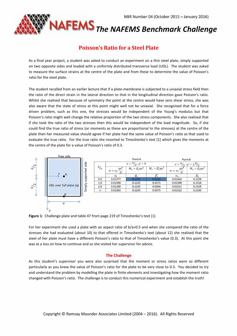
Poisson’s Ratio for a Steel Plate

As a final year project, a student was asked to conduct an experiment on a thin steel plate, simply supported

on two opposite sides and loaded with a uniformly distributed transverse load (UDL). The student was asked

to measure the surface strains at the centre of the plate and from these to determine the value of Poisson’s

ratio for the steel plate.

The student recalled from an earlier lecture that if a plate-membrane is subjected to a uniaxial stress field then

the ratio of the direct strain in the lateral direction to that in the longitudinal direction gave Poisson’s ratio.

Whilst she realised that because of symmetry the point at the centre would have zero shear stress, she was

also aware that the state of stress at this point might well not be uniaxial. She recognised that for a force

driven problem, such as this one, the stresses would be independent of the Young’s modulus but that

Poisson’s ratio might well change the relative proportion of the two stress components. She also realised that

if she took the ratio of the two stresses then this would be independent of the load magnitude. So, if she

could find the true ratio of stress (or moments as these are proportional to the stresses) at the centre of the

plate then her measured value should agree if her plate had the same value of Poisson’s ratio as that used to

evaluate the true ratio. For the true ratio she resorted to Timoshenko’s text [1] which gives the moments at

the centre of the plate for a value of Poisson’s ratio of 0.3.

Figure 1: Challenge plate and table 47 from page 219 of Timoshenko’s text [1]

For her experiment she used a plate with an aspect ratio of b/a=0.5 and when she compared the ratio of the

stresses she had evaluated (about 10) to that offered in Timoshenko’s text (about 12) she realised that the

steel of her plate must have a different Poisson’s ratio to that of Timoshenko’s value (0.3). At this point she

was at a loss on how to continue and so she visited her supervisor for advice.

The Challenge

As this student’s supervisor you were also surprised that the moment or stress ratios were so different

particularly as you knew the value of Poisson’s ratio for the plate to be very close to 0.3. You decided to try

and understand the problem by modelling the plate in finite elements and investigating how the moment ratio

changed with Poisson’s ratio. The challenge is to conduct this numerical experiment and establish the truth!



Supervisor’s Narrative As this student’s supervisor I am faced with unpicking the question she has posed me. I am pretty

convinced that the plate should have a Poisson’s ratio of 0.3 since this is the value specified by the

supplier. So what can have happened? I think the first thing to do might be to undertake an

exploration of the real solution for this problem and I can do this using a finite element model. We

have commercial finite element software in the department so let’s see if I can model this problem

and I might also take a look at the NAFEMS booklet on how to use plate elements [2]. Since

Timoshenko’s solutions deals with moments and my student is looking at surface stresses then I

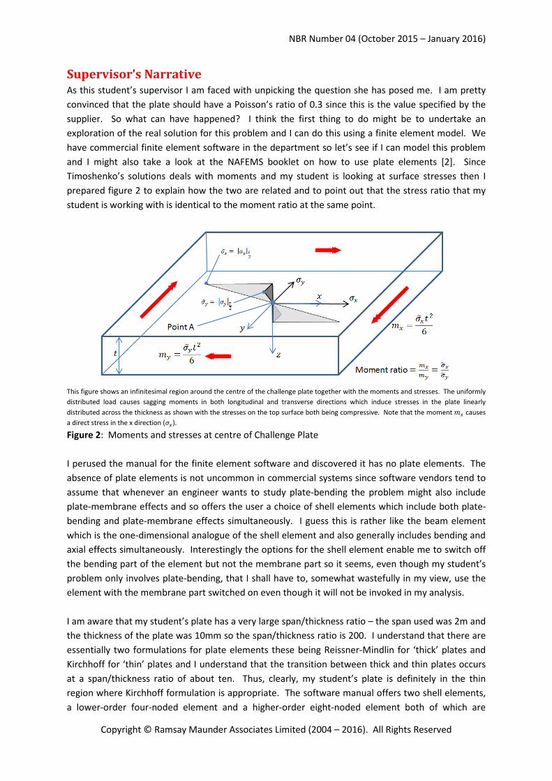
prepared figure 2 to explain how the two are related and to point out that the stress ratio that my

student is working with is identical to the moment ratio at the same point.

This figure shows an infinitesimal region around the centre of the challenge plate together with the moments and stresses. The uniformly

distributed load causes sagging moments in both longitudinal and transverse directions which induce stresses in the plate linearly

distributed across the thickness as shown with the stresses on the top surface both being compressive. Note that the moment �� causes

a direct stress in the x direction (��).

Figure 2: Moments and stresses at centre of Challenge Plate

I perused the manual for the finite element software and discovered it has no plate elements. The

absence of plate elements is not uncommon in commercial systems since software vendors tend to

assume that whenever an engineer wants to study plate-bending the problem might also include

plate-membrane effects and so offers the user a choice of shell elements which include both plate-

bending and plate-membrane effects simultaneously. I guess this is rather like the beam element

which is the one-dimensional analogue of the shell element and also generally includes bending and

axial effects simultaneously. Interestingly the options for the shell element enable me to switch off

the bending part of the element but not the membrane part so it seems, even though my student’s

problem only involves plate-bending, that I shall have to, somewhat wastefully in my view, use the

element with the membrane part switched on even though it will not be invoked in my analysis.

I am aware that my student’s plate has a very large span/thickness ratio – the span used was 2m and

the thickness of the plate was 10mm so the span/thickness ratio is 200. I understand that there are

essentially two formulations for plate elements these being Reissner-Mindlin for ‘thick’ plates and

Kirchhoff for ‘thin’ plates and I understand that the transition between thick and thin plates occurs

at a span/thickness ratio of about ten. Thus, clearly, my student’s plate is definitely in the thin

region where Kirchhoff formulation is appropriate. The software manual offers two shell elements,

a lower-order four-noded element and a higher-order eight-noded element both of which are



quoted as being suitable for thin to moderately thick shell structures so should be ideal for my

problem. The eight-noded element seems the best element to use; I always prefer to use higher-

order elements since I will need fewer elements than a lower-order equivalent element to obtain

decent results.

I will start off by modelling my student’s plate using meshes of eight-noded elements and as I am

curious to confirm the received wisdom regarding span/thickness ratios I will explore how the

moment ratio at the centre of the plate converges with mesh refinement and for different

span/thickness ratios. I will use the actual plate dimensions (2m x 1m) but I shall utilise symmetry

and model just the top right hand quadrant. Now, do I need to worry about the value of Young’s

modulus? I don’t think so because the plate problem is driven by a force (a uniformly distributed

load) and the material is isotropic so the stiffness of the material, whilst affecting the displacements,

will not influence the moments. Anyway I shall use a typical value for steel so that the deformations

are sensible.

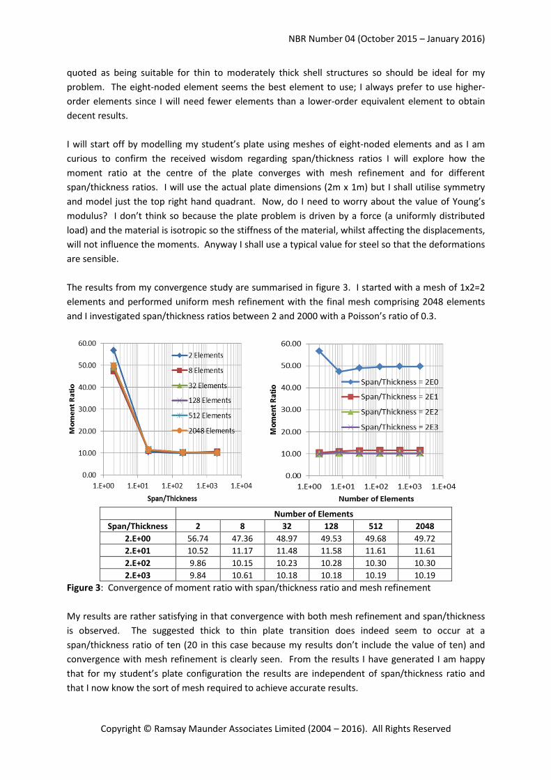
The results from my convergence study are summarised in figure 3. I started with a mesh of 1x2=2

elements and performed uniform mesh refinement with the final mesh comprising 2048 elements

and I investigated span/thickness ratios between 2 and 2000 with a Poisson’s ratio of 0.3.

Number of Elements

Span/Thickness 2 8 32 128 512 2048

2.E+00 56.74 47.36 48.97 49.53 49.68 49.72

2.E+01 10.52 11.17 11.48 11.58 11.61 11.61

2.E+02 9.86 10.15 10.23 10.28 10.30 10.30

2.E+03 9.84 10.61 10.18 10.18 10.19 10.19

Figure 3: Convergence of moment ratio with span/thickness ratio and mesh refinement

My results are rather satisfying in that convergence with both mesh refinement and span/thickness

is observed. The suggested thick to thin plate transition does indeed seem to occur at a

span/thickness ratio of ten (20 in this case because my results don’t include the value of ten) and

convergence with mesh refinement is clearly seen. From the results I have generated I am happy

that for my student’s plate configuration the results are independent of span/thickness ratio and

that I now know the sort of mesh required to achieve accurate results.



It would be interesting now to see how sensitive the moment ratio is to the following parameters:

• Poisson’s Ratio

• Aspect Ratio

• Positioning of Strain Gauge

Let me begin by considering sensitivity due to the first two parameters. I will look at aspect ratios in

the range 0.4 to 0.6 and Poisson’s ratio values in the range 0.2 to 0.4 and for each parameter I will

generate results at 0.1 intervals.

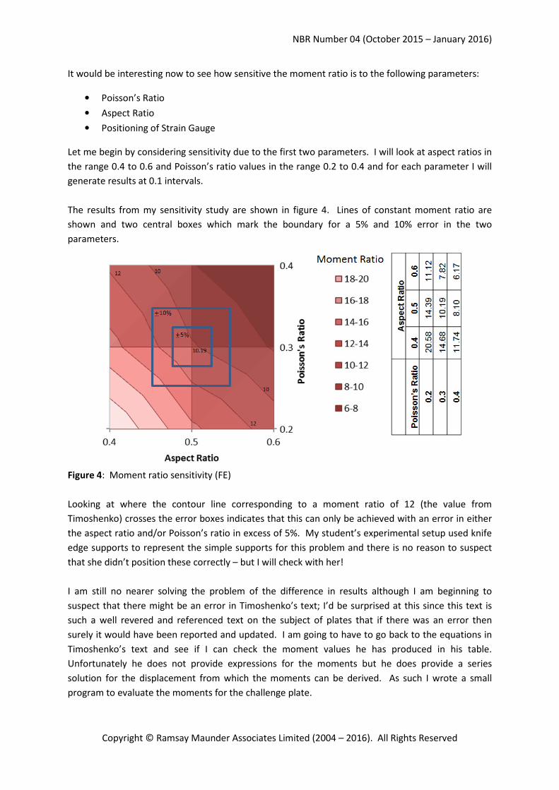
The results from my sensitivity study are shown in figure 4. Lines of constant moment ratio are

shown and two central boxes which mark the boundary for a 5% and 10% error in the two

parameters.

Figure 4: Moment ratio sensitivity (FE)

Looking at where the contour line corresponding to a moment ratio of 12 (the value from

Timoshenko) crosses the error boxes indicates that this can only be achieved with an error in either

the aspect ratio and/or Poisson’s ratio in excess of 5%. My student’s experimental setup used knife

edge supports to represent the simple supports for this problem and there is no reason to suspect

that she didn’t position these correctly – but I will check with her!

I am still no nearer solving the problem of the difference in results although I am beginning to

suspect that there might be an error in Timoshenko’s text; I’d be surprised at this since this text is

such a well revered and referenced text on the subject of plates that if there was an error then

surely it would have been reported and updated. I am going to have to go back to the equations in

Timoshenko’s text and see if I can check the moment values he has produced in his table.

Unfortunately he does not provide expressions for the moments but he does provide a series

solution for the displacement from which the moments can be derived. As such I wrote a small

program to evaluate the moments for the challenge plate.



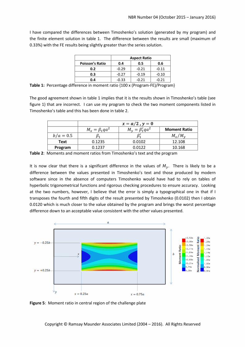
I have compared the differences between Timoshenko’s solution (generated by my program) and

the finite element solution in table 1. The difference between the results are small (maximum of

0.33%) with the FE results being slightly greater than the series solution.

Aspect Ratio

Poisson’s Ratio 0.4 0.5 0.6

0.2 -0.29 -0.21 -0.11

0.3 -0.27 -0.19 -0.10

0.4 -0.33 -0.21 -0.21

Table 1: Percentage difference in moment ratio {100 x (Program-FE)/Program}

The good agreement shown in table 1 implies that it is the results shown in Timoshenko’s table (see

figure 1) that are incorrect. I can use my program to check the two moment components listed in

Timoshenko’s table and this has been done in table 2.

� = � �⁄ , =

�� = � �� = �

�� Moment Ratio

� �⁄ = 0.5 � � � �� ⁄

Text 0.1235 0.0102 12.108

Program 0.1237 0.0122 10.168

Table 2: Moments and moment ratios from Timoshenko’s text and the program

It is now clear that there is a significant difference in the values of ��. There is likely to be a

difference between the values presented in Timoshenko’s text and those produced by modern

software since in the absence of computers Timoshenko would have had to rely on tables of

hyperbolic trigonometrical functions and rigorous checking procedures to ensure accuracy. Looking

at the two numbers, however, I believe that the error is simply a typographical one in that if I

transposes the fourth and fifth digits of the result presented by Timoshenko (0.0102) then I obtain

0.0120 which is much closer to the value obtained by the program and brings the worst percentage

difference down to an acceptable value consistent with the other values presented.

Figure 5: Moment ratio in central region of the challenge plate



I don’t want to solve my student’s problem for her and she would learn much by making the

discovery herself. If I give her my program she could use it to discover the error for herself. I could

put her off the scent a little by suggesting that she use the program to see how sensitive the

moment ratio is to the location of the strain gauges. I was rather impressed when she came back

with the diagram shown in figure 5. She explained that the moment ratio is rather insensitive to

small deviations in the location of the strain gauges and then said that if my program was correct

then there was an error in Timoshenko’s text. A great result!!

Closure This challenge has demonstrated that even in some of the most revered texts errors can occur; in

this case almost certainly the error is a typographical one. The practising engineer needs to be

aware of this and where possible take the opportunity to verify the numbers with which he/she is

presented. As demonstrated in this challenge, the finite element method is an ideal tool for the

engineer to use in this process of verification.

Having discovered an error the question now is what should the supervisor do? Well, the error in

�� at the centre of the challenge plate is about 20% and Timoshenko’s result is lower than the

correct value, i.e. it is a non-conservative prediction of the actual moment. If the engineer is using

Timoshenko’s data for the elastic design of a steel plate then he/she will spot that the highest stress

occurs at point B rather than point A (see figure 1). As there is no error in the moments at point B

then the design is not going to be compromised by this error. However, if the engineer is using

Timoshenko’s data to specify the reinforcement in a reinforced concrete slab and if he/she is looking

to optimise the reinforcement then he/she may underestimate the transverse reinforcement

requirement at the centre of the slab potentially leading to the possibility of cracking and the

necessity to rely on plastic moment redistribution in order to achieve the required strength.

The supervisor felt, as a matter of professional integrity, that he should let the publishers of

Timoshenko’s text know about the error. It appeared, though, that as no reprints of this text were

scheduled it would remain uncorrected. As such, the supervisor prepared a short article outlining

the error he had discovered and it was published both in full in the UK [3] and in a shorter version in

the US [4].

References [1] S.P. Timoshenko & S. Woinowsky-Krieger, ‘Theory of Plates and Shells’, 2

nd Edition, McGraw-Hill

International Series, 28th

Printing 1989. ISBN 0-07-Y85820-9.

[2] T. Hellen, ‘How to use Beam, Plate and Shell Elements’, NAFEMS ‘How to …’ series, Number 34, 2006.

[3] A.C.A. Ramsay & E.A.W. Maunder, ‘An Error in Timoshenko’s “Theory of Plates and Shells”’, NAFEMS

Benchmark Magazine, January 2016.

[4] A.C.A. Ramsay & E.A.W. Maunder, ‘An Error in Timoshenko’s “Theory of Plates and Shells”’, Structure

Magazine, March 2016.



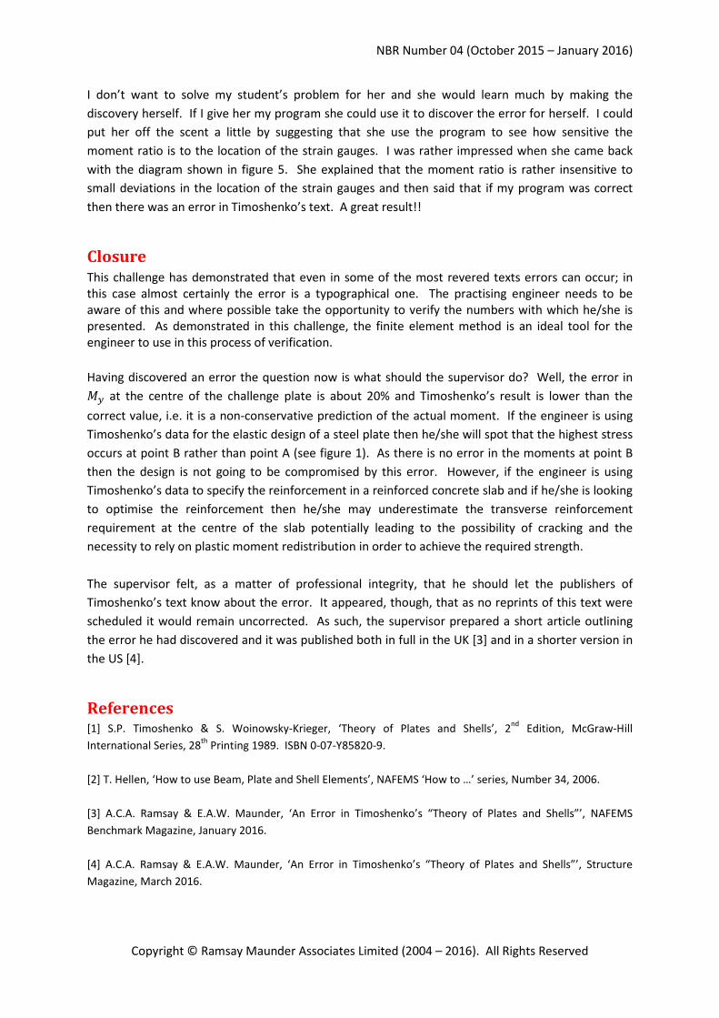
Appendix 1: Using the Program to Confirm FE Sensitivity Study The program was used to repeat the rather coarse sensitivity study conducted using the FE model

and the results are shown in figure 6.

Figure 6: Moment ratio sensitivity study (Program)

The results in figure 6 compare well with those in figure 4 and confirm the conclusions made from

the FE sensitivity study.

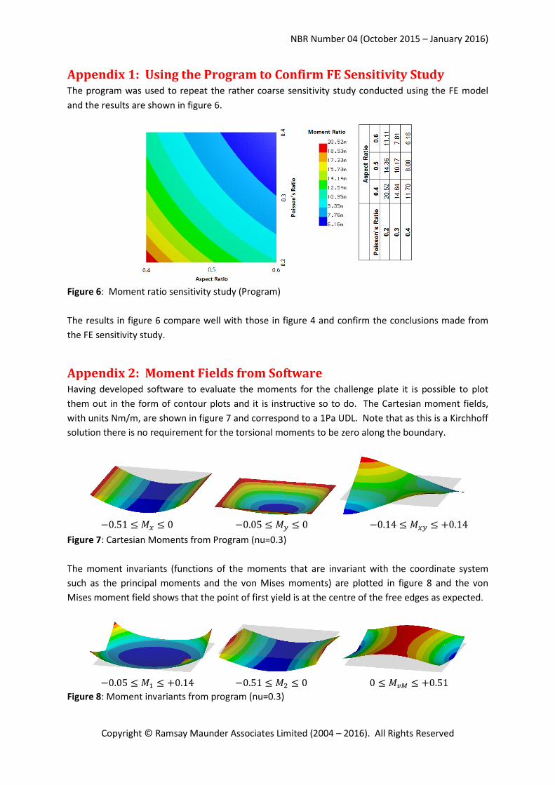
Appendix 2: Moment Fields from Software Having developed software to evaluate the moments for the challenge plate it is possible to plot

them out in the form of contour plots and it is instructive so to do. The Cartesian moment fields,

with units Nm/m, are shown in figure 7 and correspond to a 1Pa UDL. Note that as this is a Kirchhoff

solution there is no requirement for the torsional moments to be zero along the boundary.

−0.51 ≤ �� ≤ 0 −0.05 ≤ �� ≤ 0 −0.14 ≤ �� ≤ +0.14

Figure 7: Cartesian Moments from Program (nu=0.3)

The moment invariants (functions of the moments that are invariant with the coordinate system

such as the principal moments and the von Mises moments) are plotted in figure 8 and the von

Mises moment field shows that the point of first yield is at the centre of the free edges as expected.

−0.05 ≤ � ≤ +0.14 −0.51 ≤ �� ≤ 0 0 ≤ �� ≤ +0.51

Figure 8: Moment invariants from program (nu=0.3)



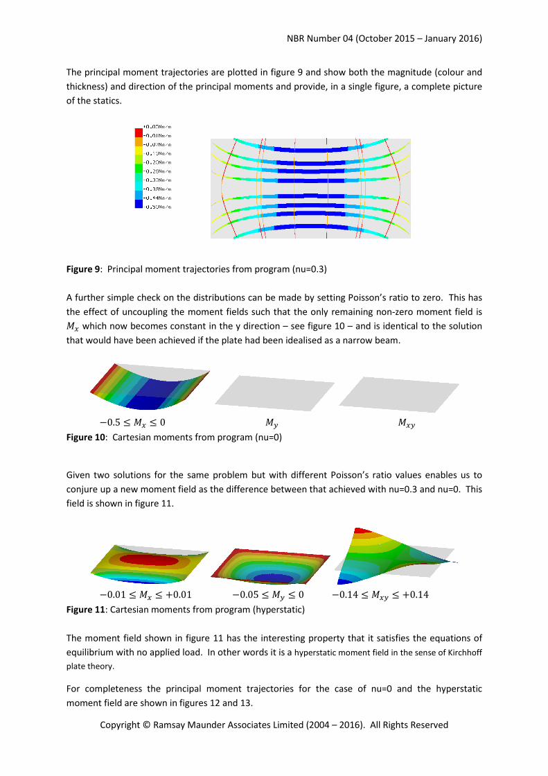
The principal moment trajectories are plotted in figure 9 and show both the magnitude (colour and

thickness) and direction of the principal moments and provide, in a single figure, a complete picture

of the statics.

Figure 9: Principal moment trajectories from program (nu=0.3)

A further simple check on the distributions can be made by setting Poisson’s ratio to zero. This has

the effect of uncoupling the moment fields such that the only remaining non-zero moment field is

�� which now becomes constant in the y direction – see figure 10 – and is identical to the solution

that would have been achieved if the plate had been idealised as a narrow beam.

−0.5 ≤ �� ≤ 0 ��

Figure 10: Cartesian moments from program (nu=0)

Given two solutions for the same problem but with different Poisson’s ratio values enables us to

conjure up a new moment field as the difference between that achieved with nu=0.3 and nu=0. This

field is shown in figure 11.

−0.01 ≤ �� ≤ +0.01 −0.05 ≤ �� ≤ 0 −0.14 ≤ �� ≤ +0.14

Figure 11: Cartesian moments from program (hyperstatic)

The moment field shown in figure 11 has the interesting property that it satisfies the equations of

equilibrium with no applied load. In other words it is a hyperstatic moment field in the sense of Kirchhoff

plate theory.

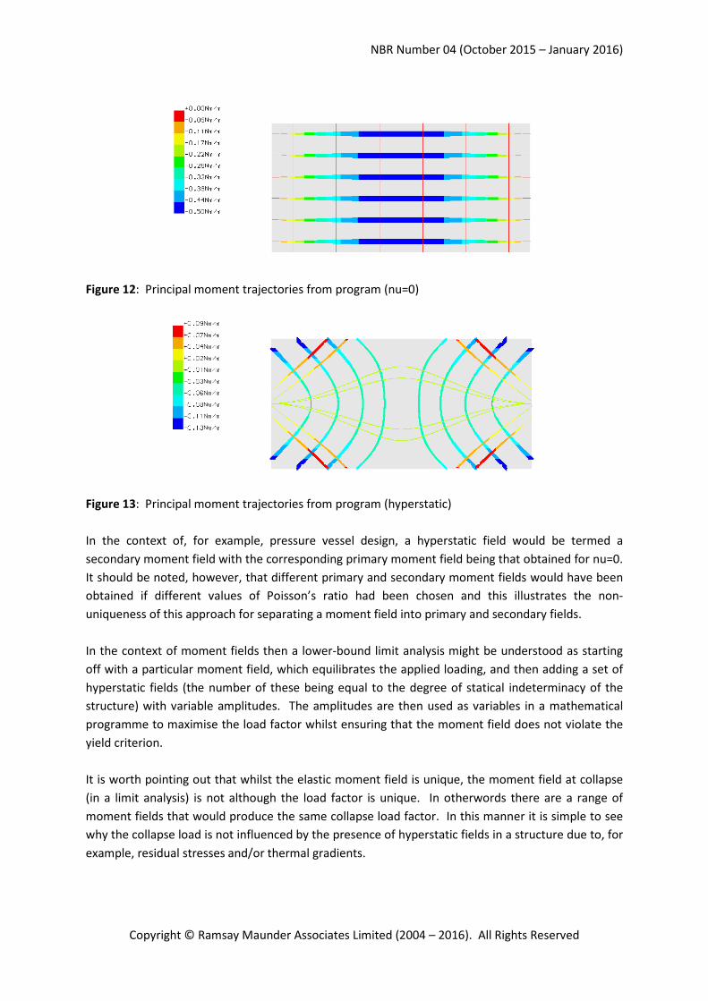
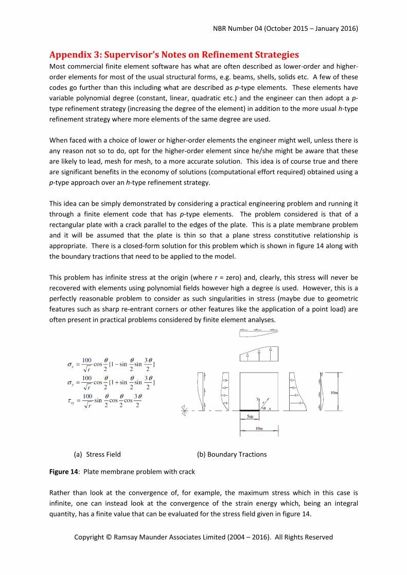
For completeness the principal moment trajectories for the case of nu=0 and the hyperstatic

moment field are shown in figures 12 and 13.



Figure 12: Principal moment trajectories from program (nu=0)

Figure 13: Principal moment trajectories from program (hyperstatic)

In the context of, for example, pressure vessel design, a hyperstatic field would be termed a

secondary moment field with the corresponding primary moment field being that obtained for nu=0.

It should be noted, however, that different primary and secondary moment fields would have been

obtained if different values of Poisson’s ratio had been chosen and this illustrates the non-

uniqueness of this approach for separating a moment field into primary and secondary fields.

In the context of moment fields then a lower-bound limit analysis might be understood as starting

off with a particular moment field, which equilibrates the applied loading, and then adding a set of

hyperstatic fields (the number of these being equal to the degree of statical indeterminacy of the

structure) with variable amplitudes. The amplitudes are then used as variables in a mathematical

programme to maximise the load factor whilst ensuring that the moment field does not violate the

yield criterion.

It is worth pointing out that whilst the elastic moment field is unique, the moment field at collapse

(in a limit analysis) is not although the load factor is unique. In otherwords there are a range of

moment fields that would produce the same collapse load factor. In this manner it is simple to see

why the collapse load is not influenced by the presence of hyperstatic fields in a structure due to, for

example, residual stresses and/or thermal gradients.



Appendix 3: Supervisor’s Notes on Refinement Strategies Most commercial finite element software has what are often described as lower-order and higher-

order elements for most of the usual structural forms, e.g. beams, shells, solids etc. A few of these

codes go further than this including what are described as p-type elements. These elements have

variable polynomial degree (constant, linear, quadratic etc.) and the engineer can then adopt a p-

type refinement strategy (increasing the degree of the element) in addition to the more usual h-type

refinement strategy where more elements of the same degree are used.

When faced with a choice of lower or higher-order elements the engineer might well, unless there is

any reason not so to do, opt for the higher-order element since he/she might be aware that these

are likely to lead, mesh for mesh, to a more accurate solution. This idea is of course true and there

are significant benefits in the economy of solutions (computational effort required) obtained using a

p-type approach over an h-type refinement strategy.

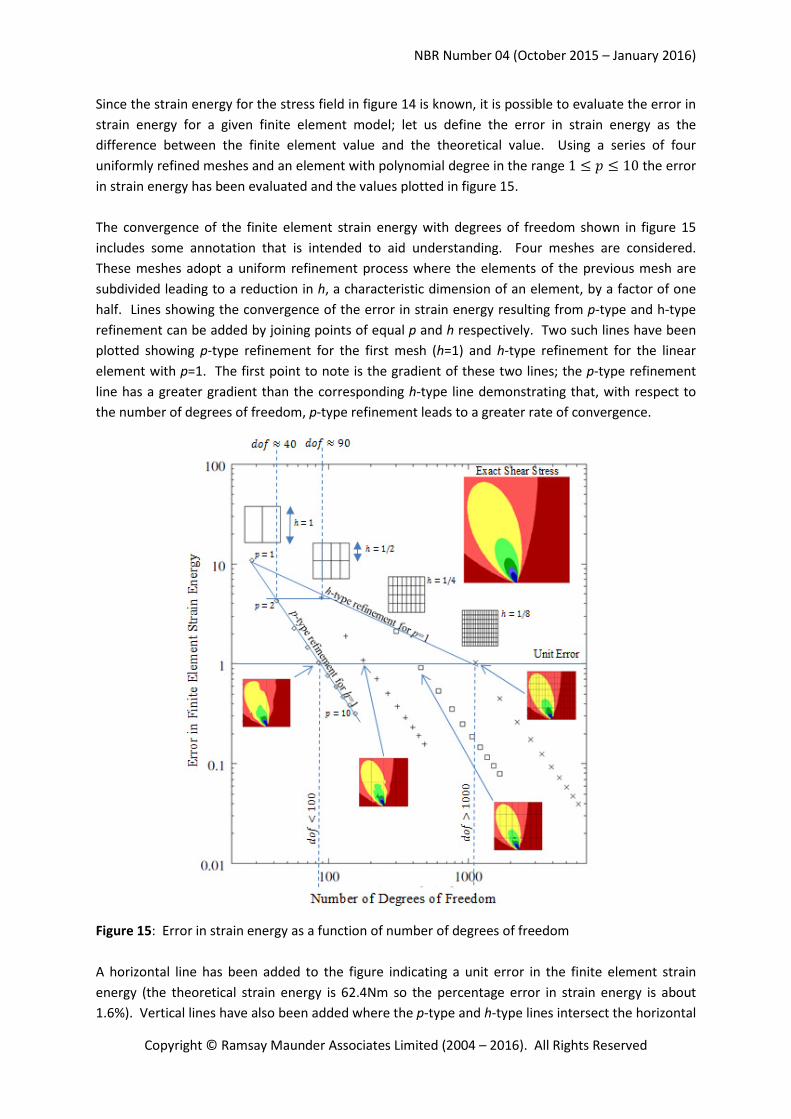
This idea can be simply demonstrated by considering a practical engineering problem and running it

through a finite element code that has p-type elements. The problem considered is that of a

rectangular plate with a crack parallel to the edges of the plate. This is a plate membrane problem

and it will be assumed that the plate is thin so that a plane stress constitutive relationship is

appropriate. There is a closed-form solution for this problem which is shown in figure 14 along with

the boundary tractions that need to be applied to the model.

This problem has infinite stress at the origin (where r = zero) and, clearly, this stress will never be

recovered with elements using polynomial fields however high a degree is used. However, this is a

perfectly reasonable problem to consider as such singularities in stress (maybe due to geometric

features such as sharp re-entrant corners or other features like the application of a point load) are

often present in practical problems considered by finite element analyses.

(a) Stress Field (b) Boundary Tractions

Figure 14: Plate membrane problem with crack

Rather than look at the convergence of, for example, the maximum stress which in this case is

infinite, one can instead look at the convergence of the strain energy which, being an integral

quantity, has a finite value that can be evaluated for the stress field given in figure 14.



Since the strain energy for the stress field in figure 14 is known, it is possible to evaluate the error in

strain energy for a given finite element model; let us define the error in strain energy as the

difference between the finite element value and the theoretical value. Using a series of four

uniformly refined meshes and an element with polynomial degree in the range 1 ≤ � ≤ 10 the error

in strain energy has been evaluated and the values plotted in figure 15.

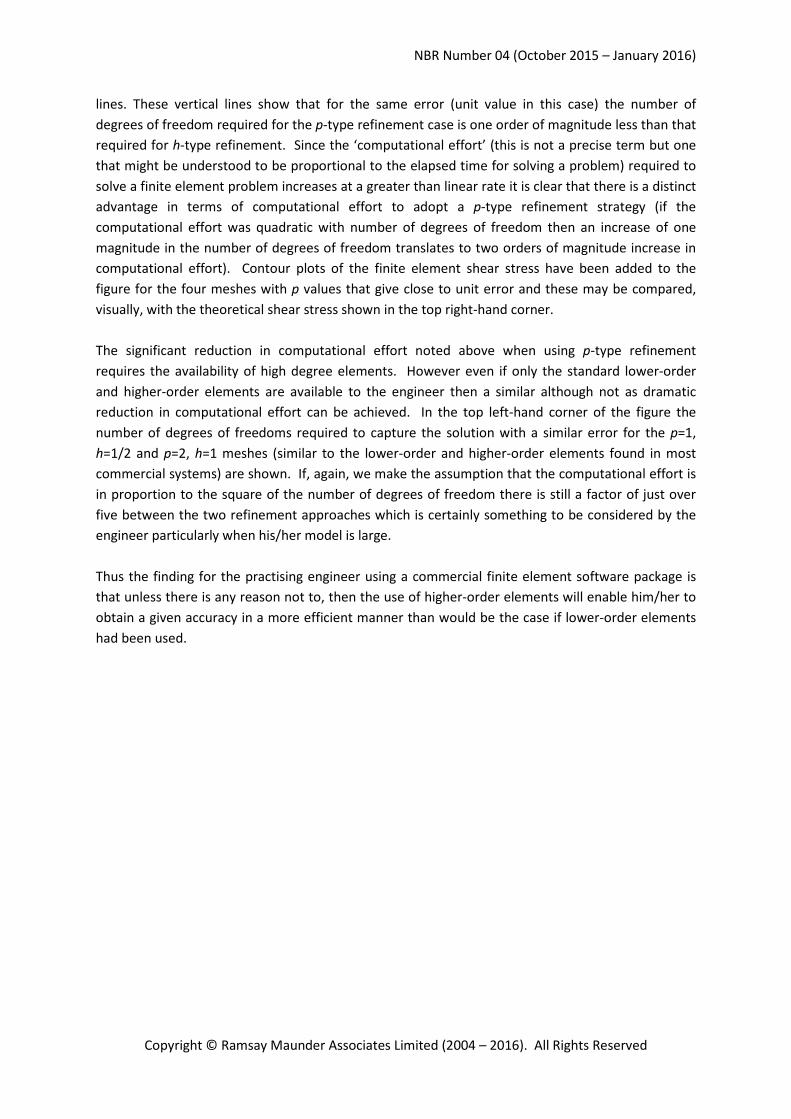
The convergence of the finite element strain energy with degrees of freedom shown in figure 15

includes some annotation that is intended to aid understanding. Four meshes are considered.

These meshes adopt a uniform refinement process where the elements of the previous mesh are

subdivided leading to a reduction in h, a characteristic dimension of an element, by a factor of one

half. Lines showing the convergence of the error in strain energy resulting from p-type and h-type

refinement can be added by joining points of equal p and h respectively. Two such lines have been

plotted showing p-type refinement for the first mesh (h=1) and h-type refinement for the linear

element with p=1. The first point to note is the gradient of these two lines; the p-type refinement

line has a greater gradient than the corresponding h-type line demonstrating that, with respect to

the number of degrees of freedom, p-type refinement leads to a greater rate of convergence.

Figure 15: Error in strain energy as a function of number of degrees of freedom

A horizontal line has been added to the figure indicating a unit error in the finite element strain

energy (the theoretical strain energy is 62.4Nm so the percentage error in strain energy is about

1.6%). Vertical lines have also been added where the p-type and h-type lines intersect the horizontal



lines. These vertical lines show that for the same error (unit value in this case) the number of

degrees of freedom required for the p-type refinement case is one order of magnitude less than that

required for h-type refinement. Since the ‘computational effort’ (this is not a precise term but one

that might be understood to be proportional to the elapsed time for solving a problem) required to

solve a finite element problem increases at a greater than linear rate it is clear that there is a distinct

advantage in terms of computational effort to adopt a p-type refinement strategy (if the

computational effort was quadratic with number of degrees of freedom then an increase of one

magnitude in the number of degrees of freedom translates to two orders of magnitude increase in

computational effort). Contour plots of the finite element shear stress have been added to the

figure for the four meshes with p values that give close to unit error and these may be compared,

visually, with the theoretical shear stress shown in the top right-hand corner.

The significant reduction in computational effort noted above when using p-type refinement

requires the availability of high degree elements. However even if only the standard lower-order

and higher-order elements are available to the engineer then a similar although not as dramatic

reduction in computational effort can be achieved. In the top left-hand corner of the figure the

number of degrees of freedoms required to capture the solution with a similar error for the p=1,

h=1/2 and p=2, h=1 meshes (similar to the lower-order and higher-order elements found in most

commercial systems) are shown. If, again, we make the assumption that the computational effort is

in proportion to the square of the number of degrees of freedom there is still a factor of just over

five between the two refinement approaches which is certainly something to be considered by the

engineer particularly when his/her model is large.

Thus the finding for the practising engineer using a commercial finite element software package is

that unless there is any reason not to, then the use of higher-order elements will enable him/her to

obtain a given accuracy in a more efficient manner than would be the case if lower-order elements

had been used.

poisson’s ratio for a steel plate - nafems · nbr number 04 (october 2015 – january 2016)...

Documents