Pitkin, M. , Doolan, S., McMenamin, L. and Wette, K. (2018) Reduced

order modelling in searches for continuous gravitational waves - I.

barycentering time delays. Monthly Notices of the Royal Astronomical

Society, 476(4), pp. 4510-4519. (doi:10.1093/mnras/sty548)

This is the author’s final accepted version.

There may be differences between this version and the published version.

You are advised to consult the publisher’s version if you wish to cite from

it.

http://eprints.gla.ac.uk/158353/

Deposited on: 22 March 2018

Enlighten – Research publications by members of the University of Glasgow

http://eprints.gla.ac.uk

Mon. Not. R. Astron. Soc. 000, 1–12 (2017) Printed March 21, 2018 (MN LATEX style file v2.2)

Reduced Order Modelling in searches for continuousgravitational waves - I. barycentering time delays

M. Pitkin1?, S. Doolan1, L. McMenamin1, K. Wette21SUPA, School of Physics and Astronomy, University of Glasgow, University Avenue, Glasgow, G12 8QQ, UK2ARC Centre of Excellence for Gravitational Wave Discovery (OzGrav) and Centre for Gravitational Physics,Research School of Physics and Engineering, The Australian National University, Canberra ACT 2601, Australia

March 21, 2018

ABSTRACTThe frequencies and phases of emission from extra-solar sources measured by Earth-bound observers are modulated by the motions of the observer with respect to thesource, and through relativistic effects. These modulations depend critically on thesource’s sky-location. Precise knowledge of the modulations are required to coherentlytrack the source’s phase over long observations, for example, in pulsar timing, orsearches for continuous gravitational waves. The modulations can be modelled as sky-location and time-dependent time delays that convert arrival times at the observer tothe inertial frame of the source, which can often be the Solar system barycentre. Westudy the use of reduced order modelling for speeding up the calculation of this timedelay for any sky-location. We find that the time delay model can be decomposedinto just four basis vectors, and with these the delay for any sky-location can bereconstructed to sub-nanosecond accuracy. When compared to standard routines fortime delay calculation in gravitational wave searches, using the reduced basis can leadto speed-ups of 30 times. We have also studied components of time delays for sourcesin binary systems. Assuming eccentricities < 0.25 we can reconstruct the delays towithin 100s of nanoseconds, with best case speed-ups of a factor of 10, or factorsof two when interpolating the basis for different orbital periods or time stamps. Inlong-duration phase-coherent searches for sources with sky-position uncertainties, orbinary parameter uncertainties, these speed-ups could allow enhancements in theirscopes without large additional computational burdens.

Key words: gravitational waves, pulsars: general, methods: data analysis

1 INTRODUCTION

When examining the frequency or phase of long-durationextra-solar astronomical sources, e.g., pulsars, as observedusing a telescope on the Earth, it is important to accountfor the frequency/phase modulation of the signal caused bythe telescope’s relative motion, and location within a grav-itational potential, with respect to the source. The relativemotion is caused by the Earth’s rotation and orbital mo-tion with respect to the Solar system barycentre (SSB), andalso any proper motion of the source compared to the SSB.Effects of general relativistic time dilation and Shapiro de-lay must also be taken into account. If searching for weaksignals, and therefore requiring coherent integration of longstretches of data, the precise knowledge of this modulationis crucial.

The coherent analysis of data over long time baselines

? matthew.pitkin@glasgow.ac.uk

is essential in determining the rotational properties of pul-sars. Generally, strong individual pulses are not seen, so thatmultiple pulses have to be folded and summed, and obser-vation periods may be short and sparsely separated, lead-ing to pulse time-of-arrival measurement that are separatedby a huge number of pulsar phase cycles. Therefore, coher-ently phase matching the pulse times requires a very precisemodel of any extrinsic and intrinsic modulations of the sig-nal. The extrinsic modulations include those caused by thechanges between the relative inertial frames of the sourceand observer, such as the motion of detector with respectto the source described above. The ability to perform thisprecise phase matching gives a form of aperture synthesiswith (for observations spanning of order a year) a baselineof the Earth’s orbital diameter, allowing very precise sky lo-calisation of sources, and good parallax and proper motionmeasurement for nearby sources.

The ability to precisely localize a source is down to thefact that the specific extrinsic modulation will very quickly

c© 2017 RAS

2 M. Pitkin

lead to decoherence of a model of the signal’s phase fromthe true signal’s phase as the model moves away from thetrue sky location. This means that for long coherent obser-vations, there will be a huge number of independent phasemodels over the sky (see, e.g., fig 14 of Wette 2014, whichshows that, when only taking sky location into considera-tion, for coherent observation of length T the number ofrequired phase models grows ∝ T q where q . 3). The cal-culation of each phase model for all the independent skypositions can be computationally demanding, so in this pa-per we study using the method of reduced order modelling(ROM) to speed-up this computation.

ROM is a term for methods that are designed to re-duce the state space dimensionality, or number of degreesof freedom, of a model in a way that it can be computedmore efficiently with a corresponding loss in accuracy. Oneoften used ROM method is Principle Component Analysisin which an orthogonal basis of model vectors is constructedfrom a set of model vectors created to cover the state spaceof possibilities. The whole orthogonal basis can be used toreconstruct any model from within the original set perfectly,whilst some subset of the basis can be found that can recon-struct any model within the initial set to a required accuracy.As the number of required bases is smaller than the origi-nal state space it often allows speed-ups in calculations ofmodels. In this paper we will use the method of producingan orthonormal reduced basis set described in section IIIof Field et al. (2014) (also see, e.g., Smith et al. 2016, fora discussion on validation and enrichment methods), whichwe will further discuss in section 2.

1.1 Searches for continuous gravitational waves

Searches for continuous sources of gravitational waves(CWs), for which the source is generally assumed to be agalactic neutron star with a non-zero mass quadrupole (i.e.,the star has a triaxial moment of inertia ellipsoid), assumequasi-monochromatic signals (see, e.g., Abbott et al. 2004,and references therein). The signals include the above men-tioned modulations and any intrinsic frequency evolutionthrough the inclusion of frequency derivative terms. Dueto the far smaller available mass quadruple, these sourcesare intrinsically weak when compared to, for example, thefinal stages of the coalescence of two black holes or neu-tron stars (see, e.g., Thorne 1987; Sathyaprakash & Schutz2009). In all-sky searches for CWs the length of data thatcan be coherently analysed is generally defined by compu-tational limitations based on the number of coherent phasetemplates required to recover signals with a certain allowableloss in recovered power (e.g. Brady et al. 1998). This compro-mise between coherent integration time and computationalresources has lead to the development of many heirarchi-cal semi-coherent search methods (see, e.g., Schutz & Papa1999; Brady & Creighton 2000; Astone et al. 2002; Krishnanet al. 2004; Abbott et al. 2008, 2009; Pletsch 2010; Wette2015; Abbott et al. 2017a, and references therein).

1.2 Solar system barycentring

The modulation of an extra-solar signal can, if working interms of signal phase, be expressed as a time modulation,

e.g., for a phase evolution given by

φ(t) = φ0 + 2πf0 (t− t0 + ∆τ(t)) , (1)

where t is the time of arrival of the signal at the observer,and φ0 and f0 are an initial phase and frequency at theepoch t0 in a reference frame at rest with respect to thesource, the time modulation term is ∆τ(t). Assuming, fornow, that the source is at rest with respect to the SSB, thetime modulation can be expressed as a combination of terms

∆τ = ∆R + ∆E −∆S , (2)

where ∆R (the Roemer delay) is a geometric retardationterm, ∆E (the Einstein delay) is a relativistic frame trans-formation term taking into account relativistic time dila-tion, and ∆S (the Shapiro delay) is the delay due to passingthrough curved space–time. These terms are discussed in,for example, chapter 5 of Lyne & Graham-Smith (1998),while Edwards, Hobbs & Manchester (2006) provide moredetailed discussion of time delays accounting for more ef-fects with particular relevance to pulsar observations. Here,for each of the terms we use the sign conventions given in thesource code for the pulsar timing software tempo21 (Hobbs,Edwards & Manchester 2006) and in the LALSuite gravita-tional wave software library functions (LIGO Scientific Col-laboration 2017), rather than those used in the equation ofEdwards, Hobbs & Manchester (2006).2 The Roemer delayis given by

∆R =r · sc, (3)

where r is a vector giving the position of the observer withrespect to the SSB, and s is a unit vector pointing fromthe observer to the source. The Einstein delay (see, e.g.,Equations 9 & 10 of Edwards, Hobbs & Manchester 2006)converts to a new time coordinate frame, and depends onthe choice of frame you want, i.e., Barycentric CoordinateTime (TCB), in which the effect of the presence of the Sun’sgravitational potential is removed. The Shapiro delay (forwhich we will only consider the contribution from the Sun)is to first order given by

∆S ≡ ∆S� = −2GM�c3

ln (rse · s + |r se|), (4)

for waves passing around the Sun, where rse = r⊕−r� is thevector from the centre of the Sun to the geocentre.3 Unlikeelectromagnetic waves, gravitational waves will pass throughmatter, and therefore a different term is required for a wave

1 https://bitbucket.org/psrsoft/tempo22 In Edwards, Hobbs & Manchester (2006) the equivalent ofEquation 1 subtracts the ∆τ term rather than adding it, andthe equivalent of Equation 2 sums all the terms. These two dif-ferences mean that the Roemer delay and Einstein delay termsin Edwards, Hobbs & Manchester (2006) have opposite signs tothose used in the source code.3 In the LALSuite (LIGO Scientific Collaboration 2017) functionsthe Shapiro delay calculation is, slightly confusingly, calculated as∆S� = 9.852×10−6 ln

(1/(r se · s + |r⊕|)

), which is equivalent

to Equation 4 with the minus sign subsumed into the logarithmterm. In tempo2 the rse is actually the vector from the Sun’scentre and the detector, rather than the geocentre. Using thegeocentre instead leads to errors on the order of 4 ns.

c© 2017 RAS, MNRAS 000, 1–12

Reduced Order Modelling for Continuous GWs 3

0.0 0.2 0.4 0.6 0.8 1.0t− t0 (yr)

0

20

40

60

80

100

120

∆S

(µs)

0.00 0.02 0.04 0.06 0.08t− t0 (yr)

200

250

300

350

400

∆R

[ge

oc

en

tre→

SSB]

(s)

15.5

15.6

15.7

15.8

15.9

∆E

(s)

−15

−10

−5

0

5

10

15

∆R

[de

tec

tor→

ge

oc

en

tre

](m

s)

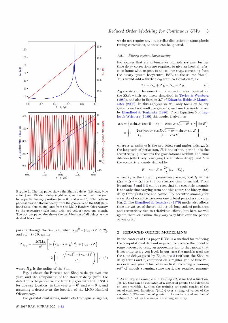
Figure 1. The top panel shows the Shapiro delay (left axis, bluecolour) and Einstein delay (right axis, red colour) over one yearfor a particular sky position (α = 0h and δ = 0◦). The bottompanel shows the Roemer delay from the geocentre to the SSB (left-hand axis, blue colour) and from the LIGO Hanford Observatoryto the geocentre (right-hand axis, red colour) over one month.The bottom panel also shows the combination of all delays as thedashed black line.

passing through the Sun, i.e., when |r se|2 − (r se · s)2 < R2�

and r se · s < 0, giving

∆S� = −2GM�c3

[ln(r se · s +

√R2� + (r se · s)2

)

− 2

1−

√|r se|2 − (r se · s)2

R�

], (5)

where R� is the radius of the Sun.Fig. 1 shows the Einstein and Shapiro delays over one

year, and the components of the Roemer delay (from thedetector to the geocentre and from the geocentre to the SSB)for one sky location (in this case α = 0h and δ = 0◦), andassuming a detector at the location of the LIGO HanfordObservatory.

For gravitational waves, unlike electromagnetic signals,

we do not require any interstellar dispersion or atmospherictiming corrections, so these can be ignored.

1.2.1 Binary system barycentring

For sources that are in binary or multiple systems, furthertime delay corrections are required to give an inertial refer-ence frame with respect to the source (e.g., correcting fromthe binary system barycentre, BSB, to the source frame).This would add a further ∆B term to Equation 2, i.e.

∆τ = ∆R + ∆E −∆S −∆B . (6)

∆B consists of the same kind of corrections as required forthe SSB, which are nicely described in Taylor & Weisberg(1989), and also in Section 2.7 of Edwards, Hobbs & Manch-ester (2006). In this analysis we will only focus on binarysystems and not multiple systems, and use the model givenby Blandford & Teukolsky (1976). From Equation 5 of Tay-lor & Weisberg (1989) this model is given as

∆B ={x sinω0 (cosE − e) +

[x cosω0

√1− e2 + γ

]sinE

}×{

1− 2πx

Pb

[cosω0 cosE√

1− e2 − sinω0 sinE]

(1− e cosE)

},

(7)

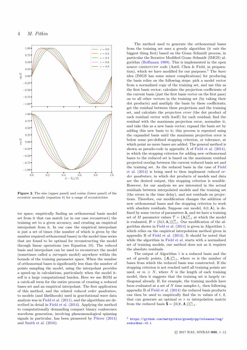
where x ≡ a sin i/c is the projected semi-major axis, ω0 isthe longitude of periastron, Pb is the orbital period, e is theeccentricity, γ measures the gravitational redshift and timedilation (effectively conveying the Einstein delay), and E isthe eccentric anomaly defined by

E − e sinE =2π

Pb(tb − T0) , (8)

where T0 is the time of periastron passage, and tb ≡ t +(∆R + ∆E − ∆S) is the barycentric time of arrival. FromEquations 7 and 8 it can be seen that the eccentric anomalyis the only time varying term and this enters the binary timedelay through its sine and cosine. The eccentric anomaly fora variety of eccentricities over one orbital period is shown inFig. 2. The Blandford & Teukolsky (1976) model also allowstime derivatives of the orbital period, longitude of periastronand eccentricity due to relativistic effects, but here we willignore them, or assume they vary very little over the periodof one orbit.

2 REDUCED ORDER MODELLING

In the context of this paper ROM is a method for reducingthe computational demand required to produce the model ofsome process, by using an approximation to that model thatis accurate to a given level. In our case the models used arethe time delays given by Equations 2 (without the Shapirodelay term) and 7, computed on a regular grid of time val-ues over one year. This relies on first producing a trainingset4 of models spanning some particular required parame-

4 As an explicit example of a training set, if we had a function,f(t;L), that can be evaluated at a vector of points t and dependson some variable, L, then the training set could consist of theset of evaluated functions f(t ;Lj) over a range of values of thevariable L. The number of points in the vector t and number ofvalues of L defines the size of a training set array.

c© 2017 RAS, MNRAS 000, 1–12

4 M. Pitkin

−1.00

−0.75

−0.50

−0.25

0.00

0.25

0.50

0.75

1.00

sinE

e = 0.0

e = 0.2

e = 0.4

e = 0.6

e = 0.8

0.0 0.2 0.4 0.6 0.8 1.0(t− T0)/Pb

−1.00

−0.75

−0.50

−0.25

0.00

0.25

0.50

0.75

1.00

cosE

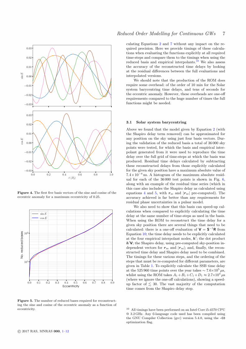
Figure 2. The sine (upper panel) and cosine (lower panel) of theeccentric anomaly (equation 8) for a range of eccentricities

ter space, empirically finding an orthonormal basis modelset from it that can match (or in our case reconstruct) thetraining set to a given accuracy, and creating an empiricalinterpolant from it. In our case the empirical interpolantis just a set of times (the number of which is given by thenumber required orthonormal bases) in the model time seriesthat are found to be optimal for reconstructing the modelthrough linear operations (see Equation 10). The reducedbasis and interpolant can be used to reconstruct the model(sometimes called a surrogate model) anywhere within thebounds of the training parameter space. When the numberof orthonormal bases is significantly less than the number ofpoints sampling the model, using the interpolant providesa speed-up in calculations, particularly when the model it-self is a large computational burden. Here we use ROM asa catch-all term for the entire process of creating a reducedbases set and an empirical interpolant. The first applicationof this method, and the related reduced order quadrature,to models (and likelihoods) used in gravitational wave dataanalysis was in Field et al. (2011), and the algorithms are de-scribed in detail in Field et al. (2014). Applying the methodto computationally demanding compact binary coalescencewaveform generation, involving phenomenological spinningsignals in particular, has been pioneered by Pürrer (2014)and Smith et al. (2016).

The method used to generate the orthonormal basesfrom the training set uses a greedy algorithm (it eats thebiggest thing first) based on the Gram–Schmidt process, inparticular the Iterative Modified Gram–Schmidt (IMGS) al-gorithm (Hoffmann 1989). This is implemented in the opensource greedycpp code (Antil, Chen & Field, in prepara-tion), which we have modified for our purposes.5 The basicidea (IMGS has some minor complications) for producingthe basis relies on the following steps: pick a model vectorfrom a normalized copy of the training set, and use this asthe first basis vector; calculate the projection coefficients ofthe current basis (just the first basis vector on the first pass)on to all other vectors in the training set (by taking theirdot products) and mutliply the basis by these coefficients;get the residual between these projections and the trainingset, and calculate the projection error (the dot product ofeach residual vector with itself) for each residual; find theresidual with the maximum projection error, normalize it,and take this as a new basis vector; expand the basis set byadding this new basis to it; this process is repeated usingthe expanded basis until the maximum projection error isbelow some pre-defined stopping criterion, or tolerance, atwhich point no more bases are added. The general method isshown as pseudo-code in appendix A of Field et al. (2014),in which the stopping criterion for adding new orthonormalbases to the reduced set is based on the maximum residualprojected overlap between the current reduced basis set andthe training set. As the reduced basis in the case of Fieldet al. (2014) is being used to then implement reduced or-der quadrature, in which dot products of models and dataare the desired output, this stopping criterion is sensible.However, for our analysis we are interested in the actualresiduals between interpolated models and the training set(the errors in the time delay), and not residuals on projec-tions. Therefore, our modification changes the addition ofnew orthonormal bases and the stopping criterion to workwith absolute residuals. Suppose our model, h(t;λ), is de-fined by some vector of parameters λ, and we have a trainingset of M parameter values T = {λ}Mi=1 at which the modelis evaluated, B = {h(t;λi)}Mi=1. Our modification of the al-gorithm shown in Field et al. (2014) is given in Algorithm 1,which relies on the empirical interpolation method given inappendix B of Field et al. (2014). It should be noted thatwhile the algorithm in Field et al. starts with a normalizedset of training models, our method does not as it requiresthe absolute residuals.

The output of Algorithm 1 is a reduced basis and theset of greedy points, {Λi}mi=1, where m is the number ofbases from which the reduced basis was constructed. If thestopping criterion is not reached until all training points areused, or m > N , where N is the length of each trainingmodel, then it suggests that the training set is largely or-thogonal already. If, for example, the training models havebeen evaluated at a set of N time samples ti, then followingappendix B of Field et al. (2014) the reduced basis productscan then be used to empirically find the m values of t, t ,that can generate an optimal m × m interpolation matrixfrom the reduced basis S = {h(t ,Λi)}mi=1.

5 https://github.com/mattpitkin/greedycpp/releases/tag/redordbar-v0.1

c© 2017 RAS, MNRAS 000, 1–12

Reduced Order Modelling for Continuous GWs 5

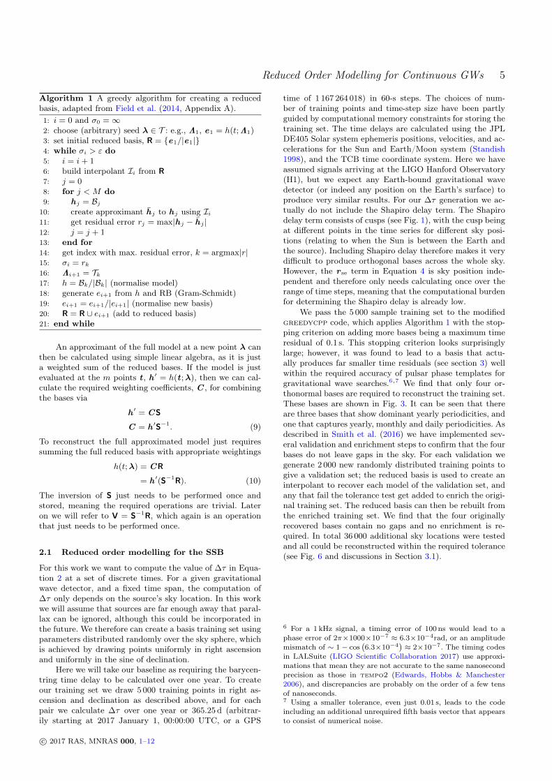
Algorithm 1 A greedy algorithm for creating a reducedbasis, adapted from Field et al. (2014, Appendix A).1: i = 0 and σ0 =∞2: choose (arbitrary) seed λ ∈ T : e.g., Λ1, e1 = h(t;Λ1)3: set initial reduced basis, R = {e1/|e1|}4: while σi > ε do5: i = i+ 16: build interpolant Ii from R7: j = 08: for j < M do9: hj = Bj

10: create approximant hj to hj using Ii11: get residual error rj = max|hj − hj |12: j = j + 113: end for14: get index with max. residual error, k = argmax|r|15: σi = rk16: Λi+1 = Tk17: h = Bk/|Bk| (normalise model)18: generate ei+1 from h and RB (Gram-Schmidt)19: ei+1 = ei+1/|ei+1| (normalise new basis)20: R = R ∪ ei+1 (add to reduced basis)21: end while

An approximant of the full model at a new point λ canthen be calculated using simple linear algebra, as it is justa weighted sum of the reduced bases. If the model is justevaluated at the m points t , h ′ = h(t ;λ), then we can cal-culate the required weighting coefficients, C , for combiningthe bases via

h ′ = CS

C = h ′S−1. (9)

To reconstruct the full approximated model just requiressumming the full reduced basis with appropriate weightings

h(t;λ) = CR

= h ′(S−1R). (10)

The inversion of S just needs to be performed once andstored, meaning the required operations are trivial. Lateron we will refer to V = S−1R, which again is an operationthat just needs to be performed once.

2.1 Reduced order modelling for the SSB

For this work we want to compute the value of ∆τ in Equa-tion 2 at a set of discrete times. For a given gravitationalwave detector, and a fixed time span, the computation of∆τ only depends on the source’s sky location. In this workwe will assume that sources are far enough away that paral-lax can be ignored, although this could be incorporated inthe future. We therefore can create a basis training set usingparameters distributed randomly over the sky sphere, whichis achieved by drawing points uniformly in right ascensionand uniformly in the sine of declination.

Here we will take our baseline as requiring the barycen-tring time delay to be calculated over one year. To createour training set we draw 5 000 training points in right as-cension and declination as described above, and for eachpair we calculate ∆τ over one year or 365.25 d (arbitrar-ily starting at 2017 January 1, 00:00:00 UTC, or a GPS

time of 1 167 264 018) in 60-s steps. The choices of num-ber of training points and time-step size have been partlyguided by computational memory constraints for storing thetraining set. The time delays are calculated using the JPLDE405 Solar system ephemeris positions, velocities, and ac-celerations for the Sun and Earth/Moon system (Standish1998), and the TCB time coordinate system. Here we haveassumed signals arriving at the LIGO Hanford Observatory(H1), but we expect any Earth-bound gravitational wavedetector (or indeed any position on the Earth’s surface) toproduce very similar results. For our ∆τ generation we ac-tually do not include the Shapiro delay term. The Shapirodelay term consists of cusps (see Fig. 1), with the cusp beingat different points in the time series for different sky posi-tions (relating to when the Sun is between the Earth andthe source). Including Shapiro delay therefore makes it verydifficult to produce orthogonal bases across the whole sky.However, the r se term in Equation 4 is sky position inde-pendent and therefore only needs calculating once over therange of time steps, meaning that the computational burdenfor determining the Shapiro delay is already low.

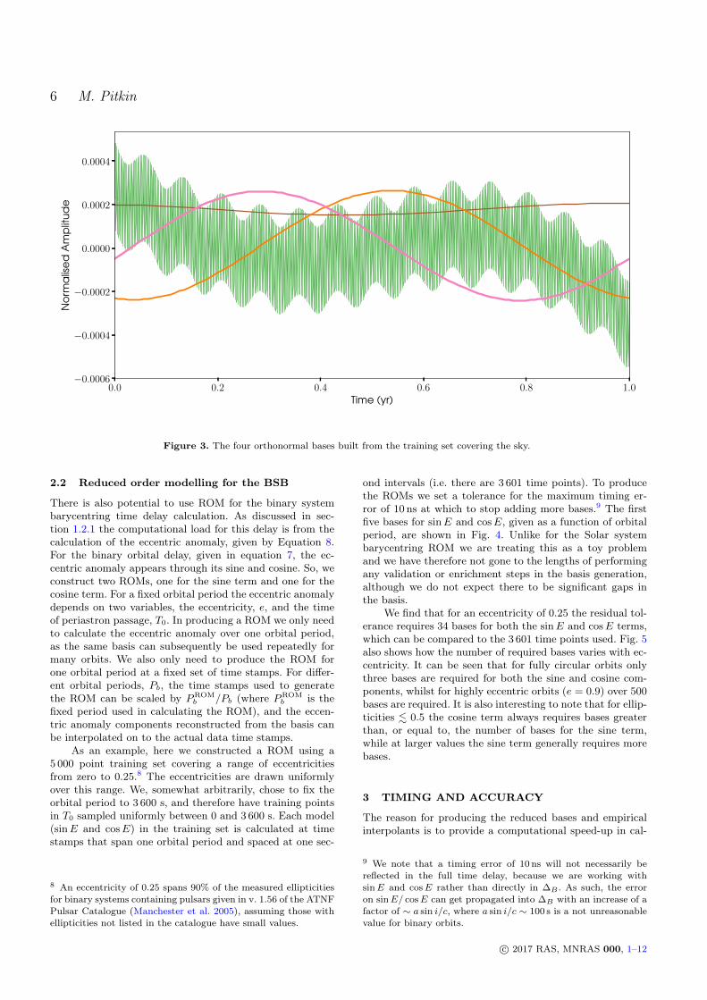
We pass the 5 000 sample training set to the modifiedgreedycpp code, which applies Algorithm 1 with the stop-ping criterion on adding more bases being a maximum timeresidual of 0.1 s. This stopping criterion looks surprisinglylarge; however, it was found to lead to a basis that actu-ally produces far smaller time residuals (see section 3) wellwithin the required accuracy of pulsar phase templates forgravitational wave searches.6,7 We find that only four or-thonormal bases are required to reconstruct the training set.These bases are shown in Fig. 3. It can be seen that thereare three bases that show dominant yearly periodicities, andone that captures yearly, monthly and daily periodicities. Asdescribed in Smith et al. (2016) we have implemented sev-eral validation and enrichment steps to confirm that the fourbases do not leave gaps in the sky. For each validation wegenerate 2 000 new randomly distributed training points togive a validation set; the reduced basis is used to create aninterpolant to recover each model of the validation set, andany that fail the tolerance test get added to enrich the origi-nal training set. The reduced basis can then be rebuilt fromthe enriched training set. We find that the four originallyrecovered bases contain no gaps and no enrichment is re-quired. In total 36 000 additional sky locations were testedand all could be reconstructed within the required tolerance(see Fig. 6 and discussions in Section 3.1).

6 For a 1 kHz signal, a timing error of 100 ns would lead to aphase error of 2π×1000×10−7 ≈ 6.3×10−4rad, or an amplitudemismatch of ∼ 1− cos

(6.3×10−4

)≈ 2×10−7. The timing codes

in LALSuite (LIGO Scientific Collaboration 2017) use approxi-mations that mean they are not accurate to the same nanosecondprecision as those in tempo2 (Edwards, Hobbs & Manchester2006), and discrepancies are probably on the order of a few tensof nanoseconds.7 Using a smaller tolerance, even just 0.01 s, leads to the codeincluding an additional unrequired fifth basis vector that appearsto consist of numerical noise.

c© 2017 RAS, MNRAS 000, 1–12

6 M. Pitkin

0.0 0.2 0.4 0.6 0.8 1.0Time (yr)

−0.0006

−0.0004

−0.0002

0.0000

0.0002

0.0004

No

rma

lise

dA

mp

litud

e

Figure 3. The four orthonormal bases built from the training set covering the sky.

2.2 Reduced order modelling for the BSB

There is also potential to use ROM for the binary systembarycentring time delay calculation. As discussed in sec-tion 1.2.1 the computational load for this delay is from thecalculation of the eccentric anomaly, given by Equation 8.For the binary orbital delay, given in equation 7, the ec-centric anomaly appears through its sine and cosine. So, weconstruct two ROMs, one for the sine term and one for thecosine term. For a fixed orbital period the eccentric anomalydepends on two variables, the eccentricity, e, and the timeof periastron passage, T0. In producing a ROM we only needto calculate the eccentric anomaly over one orbital period,as the same basis can subsequently be used repeatedly formany orbits. We also only need to produce the ROM forone orbital period at a fixed set of time stamps. For differ-ent orbital periods, Pb, the time stamps used to generatethe ROM can be scaled by PROM

b /Pb (where PROMb is the

fixed period used in calculating the ROM), and the eccen-tric anomaly components reconstructed from the basis canbe interpolated on to the actual data time stamps.

As an example, here we constructed a ROM using a5 000 point training set covering a range of eccentricitiesfrom zero to 0.25.8 The eccentricities are drawn uniformlyover this range. We, somewhat arbitrarily, chose to fix theorbital period to 3 600 s, and therefore have training pointsin T0 sampled uniformly between 0 and 3 600 s. Each model(sinE and cosE) in the training set is calculated at timestamps that span one orbital period and spaced at one sec-

8 An eccentricity of 0.25 spans 90% of the measured ellipticitiesfor binary systems containing pulsars given in v. 1.56 of the ATNFPulsar Catalogue (Manchester et al. 2005), assuming those withellipticities not listed in the catalogue have small values.

ond intervals (i.e. there are 3 601 time points). To producethe ROMs we set a tolerance for the maximum timing er-ror of 10 ns at which to stop adding more bases.9 The firstfive bases for sinE and cosE, given as a function of orbitalperiod, are shown in Fig. 4. Unlike for the Solar systembarycentring ROM we are treating this as a toy problemand we have therefore not gone to the lengths of performingany validation or enrichment steps in the basis generation,although we do not expect there to be significant gaps inthe basis.

We find that for an eccentricity of 0.25 the residual tol-erance requires 34 bases for both the sinE and cosE terms,which can be compared to the 3 601 time points used. Fig. 5also shows how the number of required bases varies with ec-centricity. It can be seen that for fully circular orbits onlythree bases are required for both the sine and cosine com-ponents, whilst for highly eccentric orbits (e = 0.9) over 500bases are required. It is also interesting to note that for ellip-ticities . 0.5 the cosine term always requires bases greaterthan, or equal to, the number of bases for the sine term,while at larger values the sine term generally requires morebases.

3 TIMING AND ACCURACY

The reason for producing the reduced bases and empiricalinterpolants is to provide a computational speed-up in cal-

9 We note that a timing error of 10 ns will not necessarily bereflected in the full time delay, because we are working withsinE and cosE rather than directly in ∆B . As such, the erroron sinE/ cosE can get propagated into ∆B with an increase of afactor of ∼ a sin i/c, where a sin i/c ∼ 100 s is a not unreasonablevalue for binary orbits.

c© 2017 RAS, MNRAS 000, 1–12

Reduced Order Modelling for Continuous GWs 7

−0.03

−0.02

−0.01

0.00

0.01

0.02

0.03

sinE

0.0 0.2 0.4 0.6 0.8 1.0t (Pb)

−0.03

−0.02

−0.01

0.00

0.01

0.02

0.03

cosE

Figure 4. The first five basis vectors of the sine and cosine of theeccentric anomaly for a maximum eccentricity of 0.25.

0.0 0.1 0.2 0.3 0.4 0.5 0.6 0.7 0.8 0.9Eccentricity

101

102

No

.re

duc

ed

ba

ses

sinE

cosE

Figure 5. The number of reduced bases required for reconstruct-ing the sine and cosine of the eccentric anomaly as a function ofeccentricity.

culating Equations 2 and 7 without any impact on the re-quired precision. Here we provide timings of these calcula-tions when evaluating the functions explicitly at all requiredtime-steps and compare them to the timings when using thereduced basis and empirical interpolants.10 We also assessthe accuracy of the reconstructed time delays by lookingat the residual differences between the full evaluations andinterpolated versions.

We should note that the production of the ROM doesrequire some overhead: of the order of 10 min for the Solarsystem barycentring time delays, and tens of seconds forthe eccentric anomaly. However, these overheads are one-offrequirements compared to the huge number of times the fullfunctions might be needed.

3.1 Solar system barycentring

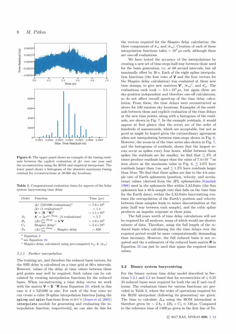
Above we found that the model given by Equation 2 (withthe Shapiro delay term removed) can be approximated forany position on the sky using just four basis vectors. Dur-ing the validation of the reduced basis a total of 36 000 skypoints were tested, for which the basis and empirical inter-polant generated from it were used to reproduce the timedelay over the full grid of time-steps at which the basis wasproduced. Residual time delays calculated by subtractingthese reconstructed delays from those explicitly calculatedfor the given sky position have a maximum absolute value of7.4×10−4 ns. A histogram of the maximum absolute resid-ual for each of the 36 000 test points is shown in Fig. 6,along with an example of the residual time series (which inthis case also includes the Shapiro delay as calculated usingequations 4 and 5, with r se and |r se| pre-computed). Theaccuracy achieved is far better than any requirements forresidual phase uncertainties in a pulsar model.

We also need to show that this basis can speed-up cal-culations when compared to explicitly calculating the timedelay at the same number of time-steps as used in the basis.When using the ROM to reconstruct the time delay for agiven sky position there are several things that need to becalculated: there is a one-off evaluation of V = S−1R fromEquation 10; the time delay needs to be explicitly calculatedat the four empirical interpolant nodes, h ′; the dot producth ′V; the Shapiro delay, using pre-computed sky-position in-dependent vectors for r se and |r se|; and, finally, the recon-structed time delay and Shapiro delay need to be combined.The timings for these various steps, and the ordering of thesteps that must be re-computed for different parameters, aregiven in Table 1. To explicitly calculate the SSB time delayat the 525 960 time points over the year takes ∼ 7.6×105 µs,whilst using the ROM takes A1 +B1 +C1 +D1 ≈ 2.7×104 µs(where we ignore the one-off calculations), showing a speed-up factor of . 30. The vast majority of the computationtime comes from the Shapiro delay step.

10 All timings have been performed on an Intel Core i5-4570 CPU@ 3.2GHz. Any C-language code used has been compiled usingthe GNU Compiler Collection (gcc) version 5.4.0, using the -O3optimization flag.

c© 2017 RAS, MNRAS 000, 1–12

8 M. Pitkin

0.0 0.2 0.4 0.6 0.8 1.0Time (yr)

−0.00050

−0.00025

0.00000

0.00025

0.00050

Tim

eRe

sidua

l(n

s)

0.0001 0.0002 0.0003 0.0004 0.0005 0.0006 0.0007Max. Time Residual (ns)

0

2000

4000

6000

8000

Figure 6. The upper panel shows an example of the timing resid-uals between the explicit evaluation of ∆τ over one year andthe reconstruction using the ROM and empirical interpolant. Thelower panel shows a histogram of the absolute maximum timingresidual for reconstructions at 36 000 sky locations.

Table 1. Computational evaluation times for aspects of the Solarsystem barycentring time delay

Order Function Time (µs)

∆τ (525 690 evaluations)a ∼ 7.6×105

∆τ (1 evaluation)a ∼ 1.4V =

(S−1R

)b ∼ 1.1×104

A1 h ′ = ∆τno Shap. (4 evaluations) ∼ 5.7

B1 (∆τ)no Shap.int = h ′V ∼ 1.6×103

C1 Shapiro delayc ∼ 2.4×104

D1 (∆τ)no Shap.int − Shapiro delay ∼ 820

a Equation 2b see Equation 10c Shapiro delay calculated using pre-computed r se & |r se|

3.1.1 Further interpolation

The training set, and therefore the reduced basis vectors, forthe SSB delay is calculated on a time grid at 60-s intervals.However, values of the delay at time values between thesegrid points may well be required. Such values can be cal-culated by creating interpolation functions for the reducedbases. When reconstructing a time delay vector we workwith the matrix V = S−1R from Equation 10, which in thiscase is 4 × 525 690 in size. For each of the four rows wecan create a cubic B-spline interpolation function [using thesplrep and splev functions from scipy’s (Jones et al. 2001)interpolate module for generating and evaluating the in-terpolation function, respectively]; we can also do this for

the vectors required for the Shapiro delay calculation: thethree components of r se and |r se|. Creation of each of theseinterpolation functions takes ∼ 105 µs each, although theseare one-off evaluations.

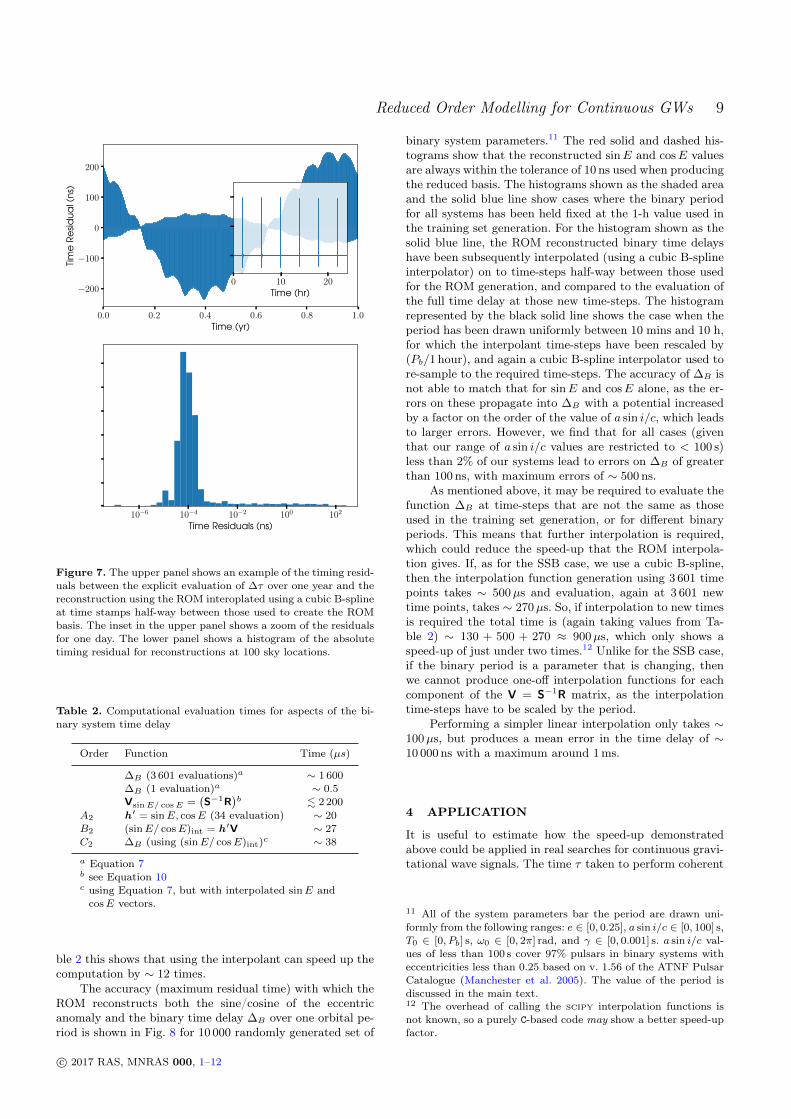
We have tested the accuracy of the interpolations bycreating a new set of time-steps half-way between those usedfor the basis generation, i.e. at 60 second intervals, but allmaximally offset by 30 s. Each of the eight spline interpola-tion functions (the four rows of V and the four vectors forthe Shapiro delay calculation) was evaluated at these newtime stamps, to give new matrices V′, |r se|′, and r ′se. Theevaluations each took ∼ 3.0×104 µs, but again these aresky-position independent and therefore one-off calculations,so do not affect overall speed-up of the time delay calcu-lation. From these, the time delays were reconstructed asabove for 100 random sky locations. Examples of the resid-uals between them and explicit evaluation of the time delaysat the new time points, along with a histogram of the resid-uals, are shown in Fig. 7. In the example residuals, it wouldappear at first glance that the errors are of the order ofhundreds of nanoseconds, which are acceptable, but not asgood as might be hoped given the extraordinary agreementwhen not interpolating between time-steps shown in Fig. 6.However, the zoom-in of the time series also shown in Fig. 7,and the histograms of residuals, shows that the largest er-rors occur as spikes every four hours, whilst between thesespikes the residuals are far smaller; we find that . 8% oftimes produce residuals larger than the value of 7.4×10−4 nsseen above as the maximum value in Fig. 6, . 2.6% haveresiduals larger than 1 ns, and . 1.2% have residuals largerthan 10 ns. We find that these spikes are due to the 4-h sam-ple rate of Earth ephemeris (position, velocity, and accela-tions) values (derived from the JPL ephemerides Standish1998) used in the ephemeris files within LALSuite (the Sunephemeris has a 40-h sample rate that falls on the time binsfor the Earth data); within the LALSuite barycentring rou-tines the extrapolation of the Earth’s position and velocitybetween these samples leads to minor discontinuities at thejoins (half way between each sample), and the cubic splineproduces an impulse response at these joins.

The full years worth of time delay calculations will notbe required for all analyses, many of which would use shortersubsets of data. Therefore, using the full length of the re-duced basis when calculating the the time delays over therequired period would be more computationally demandingthan necessary. However, the full reduced basis is not re-quired and the a submatrix of the reduced basis matrix R inEquation 10 can just be used that spans the required timesvalues.

3.2 Binary system barycentring

For the binary system time delay model described in Sec-tions 1.2.1 and 2.2 we found that for eccentricities of 6 0.2534 reduced bases were required for both the sinE and cosEterms. The evaluation times for various functions are pro-vided in Table 2, where the order of operations required forthe ROM interpolant (following its generation) are given.The time to calculate ∆B using the ROM interpolant istherefore given by ∼ 2A2 + 2B2 + C2 ≈ 130µs. Comparedto the reference time of 1 600µs given in the first line of Ta-

c© 2017 RAS, MNRAS 000, 1–12

Reduced Order Modelling for Continuous GWs 9

0.0 0.2 0.4 0.6 0.8 1.0Time (yr)

−200

−100

0

100

200

Tim

eRe

sidua

l(n

s)

10−6 10−4 10−2 100 102

Time Residuals (ns)

0 10 20Time (hr)

Figure 7. The upper panel shows an example of the timing resid-uals between the explicit evaluation of ∆τ over one year and thereconstruction using the ROM interoplated using a cubic B-splineat time stamps half-way between those used to create the ROMbasis. The inset in the upper panel shows a zoom of the residualsfor one day. The lower panel shows a histogram of the absolutetiming residual for reconstructions at 100 sky locations.

Table 2. Computational evaluation times for aspects of the bi-nary system time delay

Order Function Time (µs)

∆B (3 601 evaluations)a ∼ 1 600

∆B (1 evaluation)a ∼ 0.5

VsinE/ cosE =(S−1R

)b . 2 200

A2 h ′ = sinE, cosE (34 evaluation) ∼ 20B2 (sinE/ cosE)int = h ′V ∼ 27C2 ∆B (using (sinE/ cosE)int)c ∼ 38

a Equation 7b see Equation 10c using Equation 7, but with interpolated sinE and

cosE vectors.

ble 2 this shows that using the interpolant can speed up thecomputation by ∼ 12 times.

The accuracy (maximum residual time) with which theROM reconstructs both the sine/cosine of the eccentricanomaly and the binary time delay ∆B over one orbital pe-riod is shown in Fig. 8 for 10 000 randomly generated set of

binary system parameters.11 The red solid and dashed his-tograms show that the reconstructed sinE and cosE valuesare always within the tolerance of 10 ns used when producingthe reduced basis. The histograms shown as the shaded areaand the solid blue line show cases where the binary periodfor all systems has been held fixed at the 1-h value used inthe training set generation. For the histogram shown as thesolid blue line, the ROM reconstructed binary time delayshave been subsequently interpolated (using a cubic B-splineinterpolator) on to time-steps half-way between those usedfor the ROM generation, and compared to the evaluation ofthe full time delay at those new time-steps. The histogramrepresented by the black solid line shows the case when theperiod has been drawn uniformly between 10 mins and 10 h,for which the interpolant time-steps have been rescaled by(Pb/1 hour), and again a cubic B-spline interpolator used tore-sample to the required time-steps. The accuracy of ∆B isnot able to match that for sinE and cosE alone, as the er-rors on these propagate into ∆B with a potential increasedby a factor on the order of the value of a sin i/c, which leadsto larger errors. However, we find that for all cases (giventhat our range of a sin i/c values are restricted to < 100 s)less than 2% of our systems lead to errors on ∆B of greaterthan 100 ns, with maximum errors of ∼ 500 ns.

As mentioned above, it may be required to evaluate thefunction ∆B at time-steps that are not the same as thoseused in the training set generation, or for different binaryperiods. This means that further interpolation is required,which could reduce the speed-up that the ROM interpola-tion gives. If, as for the SSB case, we use a cubic B-spline,then the interpolation function generation using 3 601 timepoints takes ∼ 500µs and evaluation, again at 3 601 newtime points, takes ∼ 270µs. So, if interpolation to new timesis required the total time is (again taking values from Ta-ble 2) ∼ 130 + 500 + 270 ≈ 900µs, which only shows aspeed-up of just under two times.12 Unlike for the SSB case,if the binary period is a parameter that is changing, thenwe cannot produce one-off interpolation functions for eachcomponent of the V = S−1R matrix, as the interpolationtime-steps have to be scaled by the period.

Performing a simpler linear interpolation only takes ∼100µs, but produces a mean error in the time delay of ∼10 000 ns with a maximum around 1ms.

4 APPLICATION

It is useful to estimate how the speed-up demonstratedabove could be applied in real searches for continuous gravi-tational wave signals. The time τ taken to perform coherent

11 All of the system parameters bar the period are drawn uni-formly from the following ranges: e ∈ [0, 0.25], a sin i/c ∈ [0, 100] s,T0 ∈ [0, Pb] s, ω0 ∈ [0, 2π] rad, and γ ∈ [0, 0.001] s. a sin i/c val-ues of less than 100 s cover 97% pulsars in binary systems witheccentricities less than 0.25 based on v. 1.56 of the ATNF PulsarCatalogue (Manchester et al. 2005). The value of the period isdiscussed in the main text.12 The overhead of calling the scipy interpolation functions isnot known, so a purely C-based code may show a better speed-upfactor.

c© 2017 RAS, MNRAS 000, 1–12

10 M. Pitkin

10−3 10−2 10−1 100 101 102 103

Maximum Time Residual (ns)

0

500

1000

1500

2000

2500

3000sinE

cosE

∆B

∆B, Interp. t∆B, Varying Pb

Figure 8. Histograms of maximum residuals between the func-tions sinE, cosE and ∆B as explicitly evaluated and recon-structed using the ROM.

matched-filtering of a single continuous wave signal templatecan be modelled as (Prix 2017):

τ = τcore + bτbary (11)

when τcore is the time taken to perform the core filteringoperations, τbary is the time taken to perform solar systemand/or binary system barycentering. It is usual to buffer thebarycentered time series if the sky position and/or binarysystem parameters have not changed from the previously-analysed signal template; conversely when the sky positionand/or binary system parameters do change, the barycen-tered time series must be recomputed for the new param-eters. The fraction of signal templates where barycenteringmust be re-performed is denoted b. The value of b largelydepends on the design of the search algorithm and theparameter-space being searched. For search algorithms thatdo not use a search grid but rather compute templates atrandomly chosen parameters (e.g. Shaltev & Prix 2013; Shal-tev et al. 2014; Ashton 2017; Ashton & Prix 2018) we haveb = 1.

The speed-up of such a search xsearch due of the use ofa ROM may be quantified using Eqn. (11) as

xsearch =τcore + τbary

τcore + τbary/xROM

=1 + xbary

core

1 + xbarycore /xROM

(12)

where xROM is the speed-up from the use of a ROM, andxbary

core is the fraction of time spent computing the (non-ROM)barycentering, relative to performing the core filtering. Rep-resentative values of xbary

core are ∼ 17 for sky demodulationand ∼ 23 for binary demodulation.13 Given a speed-up of

13 This assumes matched filtering is performed using the demod-ulation algorithm of Williams & Schutz (2000); the FFT-basedresampling algorithm of Jaranowski, Królak & Schutz (1998) isonly efficient when searching over a wide frequency range.

xROM ∼ 30 or 12 from the use of a ROM for sky or binarydemodulation, potential search speed-ups are xsearch ∼ 11or 8 respectively.

5 CONCLUSIONS

In this paper we have aimed to show that ROM can be usedas a way to approximate the time delays required to trans-form a signal received at an observatory on Earth to the iner-tial frame of the Solar system (or binary system) barycentre.For the Solar system this transformation is sky-position de-pendent, and if requiring coherent integration of signals overlong periods its recalculation can become a computationalburden. In particular, this could be an issue for some largesky area searches for continuous gravitational wave sources,or the long-coherent time follow-up of candidates from suchsearches (Shaltev & Prix 2013; Shaltev et al. 2014; Ashton2017; Ashton & Prix 2018). We have shown that the Solarsystem barycentring time delay function can be very wellapproximated using just four basis vectors, when excludingthe Shapiro delay. Using this reduced basis can significantlyspeed up the calculation of the time delays by up to a factorof 30, even when adding on the computation of the Shapirodelay term. In general the reconstructed time delays are ac-curate to sub-nanosecond precision when compared to thefull calculation. If time delays needs to be calculated at timestamps not used for the reduced basis production, then ad-ditional interpolation of the basis vectors can be used. Inthis case it, is found that for a few percent of the samplesthe reproductions are accurate only to within ∼ 100ns. Thislarger residual has been found to be a feature of the sam-ple rate of the Solar system ephemeris files within LALSuite(LIGO Scientific Collaboration 2017).

In cases where SSB time delay calculations are a bottle-neck in analyses, for example, if having to search over a largenumber of sky positions in long data sets, this will reducethe computational burden and may allow larger parame-ter spaces to be searched. The barycentre time delay modelused in this work does not include all the components usedin, for example, the pulsar timing software tempo2 (Ed-wards, Hobbs & Manchester 2006). However, in the futureit may well be straightforward to incorporate the tempo2timing model into greedycpp (Antil et al., in preparation).In the future the timing routines in LALSuite (LIGO Sci-entific Collaboration 2017) could be adapted to incorporatethe ROMs, as produced using the tempo2 model, and thusensure consistency between the two code bases.

In addition to SSB time delays, we have also looked atthe calculations required for time delay in binary systems.The main computational burden in such calculations is theeccentric anomaly. We have shown that for eccentricities of< 0.25 a reduced basis of 34 vectors is required to reproducethe sine and cosine of the eccentric anomaly to a precisionof less than 10 ns. In the simplest cases, when not varyingthe binary orbital period, factors of ∼ 10 speed-up in thetime delay calculation are found.

Outside of the initial application of this method forcontinuous gravitational wave sources with Earth-bound de-tectors, there are other areas where it could be used. Forthird-generation gravitational wave detectors (e.g., the Ein-stein Telescope, Abernathy et al. 2011, or Cosmic Explorer,

c© 2017 RAS, MNRAS 000, 1–12

Reduced Order Modelling for Continuous GWs 11

Abbott et al. 2017b), the signals from compact binary co-alescences may be within the sensitivity bands for days, socoherent integration will have to account for Earth rota-tional and orbital motion using the delays discussed here.For future space-based gravitational wave detectors (e.g.,LISA Amaro-Seoane et al. 2013; Danzmann et al. 2017) themajority of the expected signals will be quasi-continuousand long-lived within the detector’s sensitive band. The or-bital motion of the spacecraft will need to be accountedfor when searching for signals and the ROM method ap-plied here could be very useful. This approach may also beuseful for standard pulsar timing applications, especially incases where the number of time-of-arrival observations be-come large, and sky positions need to be incorporated intoparameter fits. Methods that have to sample over parameterspaces such as temponest (Lentati et al. 2014) or bayesfit(Vigeland & Vallisneri 2014) may particularly benefit fromfaster model evaluations.

In a future paper we will study how ROM methods,and the related reduced order quadrature, can be used tospeed-up likelihood evaluations in searches for gravitationalwaves from pulsars. The method has already been appliedin the search of LIGO data for signals from known pulsarsin Abbott et al. (2017c).

ACKNOWLEDGEMENTS

This work has benefited greatly from discussions with RorySmith, and from many discussions with members of theLIGO Scientific Collaboration and Virgo Collaboration, inparticular members of the continuous waves working group.The analysis has relied on the greedycpp software (Antilet al., in preparation) and LALSuite (LIGO Scientific Col-laboration 2017). The analysis has also been greatly aidedby the use of IPython (Pérez & Granger 2007), jupyternotebooks (Kluyver et al. 2016), and Cython (Behnel et al.2011), and all plots have been produced using Matplotlib(Hunter 2007; Droettboom et al. 2017). MP is funded bythe Science & Technology Facilities Council under grantnumber ST/N005422/1. KW is supported by the AustralianResearch Council CE170100004. This paper carries LIGODocument Number LIGO-P1700373.

References

Abbott B., Abbott R., Adhikari R., et al., 2004,Phys. Rev. D, 69, 082004

Abbott B., Abbott R., Adhikari R., et al., 2008,Phys. Rev. D, 77, 022001

Abbott B., Abbott R., Adhikari R., et al., 2009,Phys. Rev. D, 79, 022001

Abbott B. P., Abbott R., Abbott T. D., et al., 2017a,Phys. Rev. D, 96, 062002

Abbott B. P., Abbott R., Abbott T. D., et al., 2017b, Clas-sical Quantum Gravity, 34, 044001

Abbott B. P., Abbott R., Abbott T. D., et al., 2017c, ApJ,839, 12

Abernathy M., Acernese F., Ajith P., et al., 2011, Einsteingravitational wave telescope conceptual design study.

Tech. Rep. ET-0106C-10, European Gravitatioanl Obser-vatory, http://www.et-gw.eu/

Amaro-Seoane P. et al., 2013, GW Notes, 6, 4Ashton G., 2017, PyFstat-v1.1.0. 10.5281/zenodo.1069408Ashton G., Prix R., 2018, arXiv:1802.05450Astone P., Borkowski K. M., Jaranowski P., Królak A.,2002, Phys. Rev. D, 65, 042003

Behnel S., Bradshaw R., Citro C., Dalcin L., Seljebotn D.,Smith K., 2011, Computing in Science & Engineering, 13,31 , http://cython.org

Blandford R., Teukolsky S. A., 1976, ApJ, 205, 580Brady P. R., Creighton T., 2000, Phys. Rev. D, 61, 082001Brady P. R., Creighton T., Cutler C., Schutz B. F., 1998,Phys. Rev. D, 57, 2101

Danzmann K., et al., 2017, LISA: Laser InterferometerSpace Antenna. https://www.elisascience.org/files/publications/LISA_L3_20170120.pdf

Droettboom M., Caswell T. A., Hunter J., et al., 2017,matplotlib/matplotlib: v2.0.0. 10.5281/zenodo.248351

Edwards R. T., Hobbs G. B., Manchester R. N., 2006, MN-RAS, 372, 1549

Field S. E., Galley C. R., Herrmann F., et al., 2011,Phys. Rev. Lett., 106, 221102

Field S. E., Galley C. R., Hesthaven J. S., et al., 2014,Phys. Rev. X, 4, 031006

Hobbs G. B., Edwards R. T., Manchester R. N., 2006, MN-RAS, 369, 655

Hoffmann W., 1989, Computing, 41, 335Hunter J. D., 2007, Computing In Science & Engineering,9, 90

Jaranowski P., Królak A., Schutz B. F., 1998, Physical Re-view D, 58, 063001

Jones E., Oliphant T., Peterson P., et al., 2001, SciPy:Open source scientific tools for Python. http://www.scipy.org/

Kluyver T. et al., 2016, in Positioning and Power in Aca-demic Publishing: Players, Agents and Agendas: Proceed-ings of the 20th International Conference on ElectronicPublishing, Loizides F., Schmidt B., eds., IOS Press, p. 87,http://jupyter.org/

Krishnan B., Sintes A. M., Papa M. A., Schutz B. F., FrascaS., Palomba C., 2004, Phys. Rev. D, 70, 082001

Lentati L., Alexander P., Hobson M. P., et al., 2014, MN-RAS, 437, 3004, https://github.com/LindleyLentati/TempoNest

LIGO Scientific Collaboration, 2017, LALSuite. https://wiki.ligo.org/DASWG/LALSuite

Lyne A. G., Graham-Smith F., 1998, Pulsar Astronomy,2nd edn., 31. Cambridge University Press

Manchester R. N., Hobbs G. B., Teoh A., HobbsM., 2005, AJ, 129, 1993, http://www.atnf.csiro.au/people/pulsar/psrcat/

Pérez F., Granger B. E., 2007, Computing in Science andEngineering, 9, 21, http://ipython.org

Pletsch H. J., 2010, Phys. Rev. D, 82, 042002Prix R., 2017, Characterizing timing and memory-requirements of the f-statistic implementations in lalsuite.Tech. Rep. LIGO-T1600531, LIGO

Pürrer M., 2014, Classical and Quantum Gravity, 31,195010

Sathyaprakash B. S., Schutz B. F., 2009, Living Rev. Rel-ativ., 12, 2

c© 2017 RAS, MNRAS 000, 1–12

12 M. Pitkin

Schutz B. F., Papa M. A., 1999, arXiv:gr-qc/9905018Shaltev M., Leaci P., Papa M. A., Prix R., 2014,Phys. Rev. D, 89, 124030

Shaltev M., Prix R., 2013, Phys. Rev. D, 87, 084057Smith R., Field S. E., Blackburn K., et al., 2016,Phys. Rev. D, 94, 044031

Standish E. M., 1998, JPL Planetary and LunarEphemerides, DE405/LE405. NASA Jet Propulsion Lab-oratory, Pasadena, IOM 312.F-98-048

Taylor J. H., Weisberg J. M., 1989, ApJ, 345, 434Thorne K. S., 1987, in Three hundred years of gravita-tion, Hawking S. W., Israel W., eds., Cambridge Univer-sity Press

Vigeland S. J., Vallisneri M., 2014, MNRAS, 440, 1446,https://github.com/vallis/mc3pta/tree/master/bayesfit

Wette K., 2014, Phys. Rev. D, 90, 122010Wette K., 2015, Phys. Rev. D, 92, 082003Williams P. R., Schutz B. F., 2000, in AIP Conference Se-ries, Meshkov S., ed., Vol. 523, pp. 473–476

c© 2017 RAS, MNRAS 000, 1–12