physiological detection of emotional states in children

i

Physiological Detection of Emotional States in Children

with Autism Spectrum Disorder (ASD)

by

Sarah Sarabadani

A thesis submitted in conformity with the requirements

for the degree of Master of Applied Science

Department of Biomaterials and Biomedical Engineering

University of Toronto

© Copyright by Sarah Sarabadani 2016

i

Physiological Detection of Emotional States in Children with

Autism Spectrum Disorder (ASD)

Sarah Sarabadani

Master of Applied Science

Department of Biomaterials and Biomedical Engineering

University of Toronto

2016

Abstract

Autism spectrum disorder (ASD) is associated with difficulties in emotion processing including

attributing emotional states to others and processing of one’s own emotional experiences. These

difficulties are linked to core social impairments and increased severity of psychiatric co-

morbidities such as depression. The nature of these difficulties has remained largely unknown.

This is partially due to limitations in obtaining reliable self report of emotional experiences in

this population.

Emotion detection using physiological signals is a promising direction in addressing this

limitation. Physiological signals can provide a language free method for understanding emotional

states in ASD. The use of this approach has not been studied in ASD.

To this end we develop a physiological approach to detection of emotion in children with ASD.

We showed that emotional states can be classified with accuracies>80% in a sample of children

with ASD which affirms the feasibility of discriminating affective states in this population.

ii

iii

Acknowledgments

Foremost, I would like to express my sincere gratitude to my thesis advisor Dr. Azadeh Kushki

for her patience, motivation, enthusiasm, and immense knowledge. Her guidance helped me in

all the time of research and writing of this thesis. She always steered me in the right direction

whenever she thought I needed it.

Besides my advisor, I would like to thank the rest of my thesis committee: Dr. Jose Zariffa, Dr.

Evdokia Anagnostou, and Dr. Azadeh Yadollahi, for their encouragement and insightful

comments.

My sincere thank also goes to Ali Samadani who always was there to answer my endless

questions. I am gratefully indebted to his very valuable helps with this thesis.

I would like to thank members of Autism Research Centre (ARC), especially Stephanie Chow

who has always supported me and helped me putting pieces together.

Finally, I must express my very profound gratitude to my parents for providing me with unfailing

support and continuous encouragement throughout my years of study and through the process of

researching and writing this thesis. This accomplishment would not have been possible without

them. Thank you.

iv

Table of Contents

Abstract ........................................................................................................................................... ii

Acknowledgments.......................................................................................................................... iii

Table of Contents ........................................................................................................................... iv

List of Tables ................................................................................................................................. vi

List of Figures ............................................................................................................................... vii

Introduction ................................................................................................................................... 1

1.1 Motivation ........................................................................................................................ 1

1.2 Research Question and Objective .................................................................................... 2

Background ................................................................................................................................... 3

2.1 Brain Activity in Emotion Processing .............................................................................. 3

2.2 Emotion Recognition in ASD .......................................................................................... 4

2.3 Automatic Emotion Recognition ...................................................................................... 5

2.4 Emotional model .............................................................................................................. 6

2.4.1 Choice of the emotion model .................................................................................... 7

2.5 Emotion elicitation ........................................................................................................... 8

2.6 Physiological Signals for Emotion Classification ............................................................ 9

2.6.1 Electrocardiogram (ECG) ......................................................................................... 9

2.6.2 Skin Conductance (SC) ........................................................................................... 10

2.6.3 Respiration (RSP) ................................................................................................... 11

2.6.4 Skin temperature (SKT) .......................................................................................... 12

2.7 Existing Systems for Physiological Emotion Recognition ............................................ 12

2.7.1 Typically developing .............................................................................................. 12

2.7.2 ASD......................................................................................................................... 14

Research Methods ....................................................................................................................... 15

3.1 Participants ..................................................................................................................... 15

3.2 Instrumentation............................................................................................................... 16

3.3 Stimuli ............................................................................................................................ 17

v

3.4 Experimental protocol .................................................................................................... 20

Analysis ........................................................................................................................................ 22

4.1 Pre-processing ................................................................................................................ 23

4.2 Feature Extraction .......................................................................................................... 24

4.3 Feature selection ............................................................................................................. 26

4.4 Classification .................................................................................................................. 27

4.5 Performance Evaluation ................................................................................................. 28

Results .......................................................................................................................................... 29

5.1 Participants Demographics ............................................................................................. 29

5.2 SAM Results .................................................................................................................. 30

5.3 Classification Results ..................................................................................................... 35

5.4 Ensemble of Classifiers .................................................................................................. 37

5.5 Classification over arousal axis ...................................................................................... 41

5.6 Modality Specific Results .............................................................................................. 42

5.7 Selected Features ............................................................................................................ 43

5.9 Association of Classification Accuracy and SAM Ratings with Demographics ........... 49

5.10 Effect of Window Size on Accuracy .............................................................................. 52

Discussion and Conclusion ......................................................................................................... 54

6.1 SAM assessment ............................................................................................................ 54

6.2 Feature selection ............................................................................................................. 55

6.3 Classification Results ..................................................................................................... 56

6.4 Effect of demographic variables/behavioural measures on accuracy ............................ 57

Conclusion ................................................................................................................................... 59

References .................................................................................................................................... 61

vi

List of Tables

Table 2.1: Summary of studies on typical individuals .................................................................. 12

Table 3.1: Average rating of final selection of pictures ................................................................ 19

Table 4.1: summary of features, SC: Skin Conductance, ECG: Electrocardiogram .................... 25

Table 5.1: Demographic information ............................................................................................ 29

Table 5.2: Overall SAM results for each participant .................................................................... 30

Table 5.3: Emotion specific SAM results for each participant ..................................................... 30

Table 5.4: Emotion specific SAM results for each parent ............................................................ 31

Table 5.5: Confusion matrix for child SAM ratings ..................................................................... 32

Table 5.6: Confusion matrix for parent SAM ratings ................................................................... 33

Table 5.7: Top ten selected features ............................................................................................. 44

Table 5.8: Accuracy of comparing HP vs. HN for each classifier ................................................ 35

Table 5.9: Accuracy of comparing LP vs. LN .............................................................................. 36

Table 5.10: Classification results of ensemble of methods ........................................................... 37

Table 5.11: Comparing un-weighted and weighted ensemble of classifiers ................................ 38

Table 5.12: Classification results using shuffled labels ................................................................ 39

Table 5.13: Confusion matrices of ensemble of methods ............................................................. 40

vii

List of Figures

Figure 2.1: Discrete and dimensional model [29] ....................................................................... 7

Figure 2.2: SAM [30] .................................................................................................................. 8

Figure 2.3: Example of a QRS waveform in an ECG signal [54] ............................................. 10

Figure 2.4: SC signal [56] ......................................................................................................... 11

Figure 2.5: respiration sensor [61] ............................................................................................ 11

Figure 2.6: Skin temperature sensor [62] .................................................................................. 12

Figure 3.1: Attachment of sensors, Procomp Infiniti hardware manual [65] ............................ 16

Figure 3.2: experimental setup .................................................................................................. 17

Figure 3.3: Procedure of picture selection ................................................................................ 19

Figure 3.4: Experimental protocol ............................................................................................ 21

Figure 4.1: Analysis procedure ................................................................................................. 23

Figure 4.2: Segmentation of each task ...................................................................................... 24

Figure 5.1: Selected features, I will replace figures with larger and clear ones later ............... 44

Figure 5.2: Selected feature for each participant.(a) low arousal, (b) high arousal, (c)

subtracting a from b................................................................................................................... 48

Figure 5.3: Bar plot of results of ensemble of classifiers .......................................................... 41

1

Chapter 1

Introduction

1.1 Motivation

Autism spectrum disorder (ASD) is a neurodevelopmental disorder characterized by social

communication difficulties and the presence of repetitive and restricted behaviors and interests

[1]. ASD is also associated with difficulties in emotion processing, which may underlie some of

the core social impairments in this population [2]. A large body of literature has examined

emotion processing in ASD, suggesting difficulties in attributing mental and emotional states to

others [3, 4, 5]. A few studies have also reported self-awareness and atypical processing of self

emotional experiences in this population [6]. For example, one in two individuals with ASD is

suggested to be affected by alexithymia (difficulties in distinguishing and describing internal

body states) [7]. This is significantly higher than the one in ten prevalence of alexithymia in the

general population [8], [9]. In addition to being closely linked to the core social impairments in

ASD [10], difficulties in interpreting and processing emotions in ASD are known to be

associated with increased severity of psychiatric disorders such as depression [2]. Hence,

assisting individuals with ASD with perceiving and processing their internal body state is

essential.

Emotion detection using physiological signals is a promising direction in addressing this gap. In

this context, a physiological approach to detection of emotions can provide a language-free, non-

invasive, and low-cost way for characterization of emotional states in children with ASD. This

work can ultimately contribute to improving self-awareness of emotions by providing users with

information regarding their actual body state. In addition it will enhance our understanding of

ASD-related emotion processing difficulties.

2

Physiological signals reflect the activity of the Autonomic Nervous System (ANS) [19]. ANS is

responsible for involuntary control of organs and regulating processes such as heart rate and

respiration [20]. Emotional stimuli have been shown to influence the activity of the ANS in a

measureable way [21]. For example, heart rate and blood pressure tend to increase in response to

anger [22].

There is extensive body of literature on characterizing physiological signals to discern emotional

states in typically developed individuals [16, 31, 32, 34, 36]. However, it is unclear that these

methods can be used in this population as ASD is associated with atypical ANS function [45].

1.2 Research Question and Objective

This research aims to answer this question: Is it possible to physiologically differentiate affective

states in children with ASD?

The goal of this study is to develop tools for physiological detection of emotions in children with

ASD. The specific objective is to develop classification techniques to differentiate patterns of

physiological response to four emotional states (high arousal/positive valence, low

arousal/positive valence, high arousal/negative valence, and low arousal/negative valence).

3

Chapter 2

Background

In this chapter we review previous research in the field of emotion recognition. First the

influence of affective state on various physiological signals is discussed. Afterwards, emotion

processing in ASD is investigated from a neurophysiologic perspective. Then, various modalities

in automatic emotion recognition including facial expressions, voice, and physiological signals

are explained and the choice of latter one is justified. Finally, three principal matters in

developing automatic emotion recognition comprising emotional model, emotion elicitation

method, and specific physiological indices of ANS activity are discussed in the following three

sections.

2.1 Brain Activity in Emotion Processing

ANS is one of the divisions of peripheral nervous system (PNS) that controls the involuntary

function of organs. It consists of two branches; the sympathetic nervous system which is known

as “fight or flight” system, activated in fast changes and arousal while inhibits digestion. The

other branch of ANS named parasympathetic nervous system which is known as “rest and

digest” system. It is associated with calming and regular function of the nerves and promoting

digestion. The function of these two parts is opposite and as one of them enhances the

physiological response, the other inhibits it [60].

There are various positions on autonomic response organization in emotion. It has been shown

that valence specific patterns are more consistent with ANS activity than discrete emotion

patterns [61]. James [62] has defined emotion as feeling of the body changes as they occur. He

has argued that emotional states are associated with specific physiological response with

4

variations in symptoms between individuals. Stemmler [65] has stated that autonomic activity

occurs prior to any behavioral changes due to emotional states. This argument is supported by

studies on paralyzed animals where there is lack of external behavior while autonomic activation

has been detected [66]. It contradicts the notion of ANS activity as a result of motoric response

[67]. Stemmler also has suggested that for body protection and behavioral adaptation distinct

autonomic response is required to exist.

A large body of literature has examined the relation between affective states and patterns in

autonomic response. They could successfully show such patterns exist in various emotional

states. As one of the pioneers in this area, Ekman [23] has investigated emotion specific

activities in ANS. He has considered six emotions (surprise, disgust, sadness, anger, fear, and

happiness) and recorded signals of heart activity, skin temperature, skin resistance, and muscle

tension. The changes were observed not only between positive and negative emotions, but also in

various negative affective states. Picard [16] also could differentiate eight discrete emotions

(neutral, anger, hate, grief, platonic love, romantic love, joy, and reverence), looking at ANS

activity through four physiological signals (i.e. muscle tension, heart activity, skin conductance,

and respiration). In another study Kim J [39] has shown there is discernible pattern between

positive/high arousal, negative/high arousal, positive/low arousal, and negative/low arousal. He

has employed four physiological signals to measure heart activity, skin conductance, respiration

rate, and muscle tension. Kim K.H [44] has also indicated pattern between sadness, anger, stress,

and surprise using signals representing heart activity, skin conductance, and temperature. These

major findings along with tons of similar works suggest that detecting pattern in physiological

signals in various emotional states is feasible.

2.2 Emotion Recognition in ASD

ASD is associated with difficulties in identify and describing one's own emotions (alexithymia

[6]). These atypicalities are suggested to be closely linked to the capacity to empathize, a key

area of difficulty in ASD.

5

Lambie and Marcel [11] conceptualized the emotion experience using a two-level model. In this

model, first-order experience of emotion is attributed to neurophysiological arousal associated

with emotional states. Self-awareness of this arousal is second-order experience of emotion

(interoception). In ASD, atypicalies have been reported both levels of emotional experience.

While emotion-related physiological arousal is suggested to be present in ASD [12], its pattern

may be atypical [13]. Interestingly, in a study by Silani et al. [6] reduced emotional awareness

was not found to be associated with reduced response in the brain regions mapped to first order

experience (amygdala and inferior orbitofrontal cortex), suggesting that this circuitry may not

underlie alexithymia symptoms in ASD [6]. Several studies have also reported that the second-

order emotional experience (i.e., aware of bodily states) is atypical in ASD [9, 12, 14, 15]. For

example, in a functional MRI study of individuals with ASD, Silani et al. [6] found a significant

negative correlation between the severity of alexithymia tendencies and activity in brain regions

associated with interoception (e.g., the insula). The authors then concluded that the lack of

awareness of bodily states, or the decoupling between physiological arousal and conscious

representation of emotions, may underlie alexithymia tendencies in ASD.

2.3 Automatic Emotion Recognition

Inferring emotional states automatically by means of computer algorithms has been studied

extensively, mainly in the context of enhancing human-computer interaction [16]. These

algorithms employ changes in internal or external states of users for emotion recognition. The

states commonly considered include facial expressions, voice, and physiological signals.

Emotion detection based on facial expressions has been mainly used for enhancing human-

computer interaction as this approach requires the user to be directly in the field of view of a

camera [17]. ASD has been associated with atypical facial expressions, which may affect the

accuracy of these methods.

Emotion detection based on voice also presents several challenges in the context of this proposal.

First, such a method requires the continuous presence of verbal expression, which may not be

possible for some individuals with ASD. Second, ASD is associated with atypical speech

6

features such as prosody [18], which may affect the recognition accuracy of these methods.

Finally, voice-based emotion detection will not be appropriate for settings, such as classrooms,

where noise is present in the environment or users do not continuously produce speech.

Emotion detection based on physiological signals is especially appropriate for use in this project

for three reasons: 1) this measurement modality can be employed across different environments

and especially in naturalistic settings; 2) physiological signals are relatively independent of

individuals ability profiles and cultural norms; 3) these signals can be measured non-invasively

and with low-cost with relatively low burden on the user. For these reasons, the physiological

approach to emotion detection is chosen for the proposed project. Three key issues need to be

considered in developing automatic emotion recognition namely, choosing the emotional model,

emotion elicitation method, and specific physiological indices of ANS activity. Details are

provided in sections that follow.

2.4 Emotional model

Two approaches are commonly used for quantitative modeling of emotions. The first, proposed

by Ekman [23], assumes the existence of a discrete set of emotions. Building on this assumption,

six classes of emotions (happiness, sadness, surprise, anger, disgust, and fear [24] have been

commonly used in the literature.

The second model of emotion challenges the discrete nature of emotion and proposes a

continuous space in two dimensions of arousal and valence [25]. Valence represents the

pleasantness of an emotion and ranges from negative to positive. Arousal reflects intensity of an

emotion and ranges from low to high. For example, happiness has positive valence and high

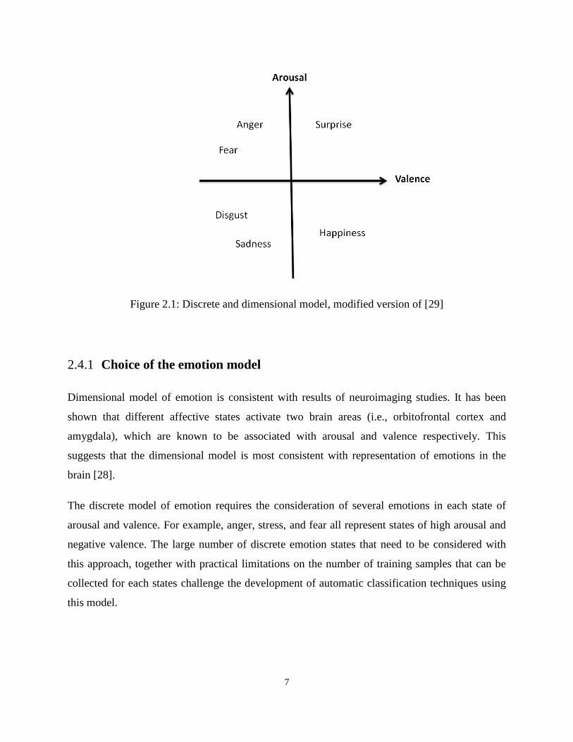
arousal, while sadness has negative valence and low arousal. Six core emotions are shown in the

valence-arousal coordinates in Figure 2.1.

7

Figure 2.1: Discrete and dimensional model, modified version of [29]

2.4.1 Choice of the emotion model

Dimensional model of emotion is consistent with results of neuroimaging studies. It has been

shown that different affective states activate two brain areas (i.e., orbitofrontal cortex and

amygdala), which are known to be associated with arousal and valence respectively. This

suggests that the dimensional model is most consistent with representation of emotions in the

brain [28].

The discrete model of emotion requires the consideration of several emotions in each state of

arousal and valence. For example, anger, stress, and fear all represent states of high arousal and

negative valence. The large number of discrete emotion states that need to be considered with

this approach, together with practical limitations on the number of training samples that can be

collected for each states challenge the development of automatic classification techniques using

this model.

8

2.5 Emotion elicitation

The most commonly stimuli in emotion detection studies in typically developing population is

using International Affective Picture System (IAPS) [31, 32, 33, 34] which is a large set of color

pictures validated to be effective for inducing different levels of arousal and valence [30]. It also

has been used in ASD [12]. For rating the pictures a visual scale, called the self assessment

manikin (SAM), has been suggested by the publishers of IAPS (Figure 2.2). The first and second

rows of SAM correspond to level of valence and arousal which were previously defined. The

third row represents dominance of emotion denoting the level of control vs. the level of being

controlled. For instance, fear and anger both are negative emotions. Regarding dominance

dimension the former is more submissive while the latter is more dominant. Geneva affective

picture database (GAPED) is a relatively new system consisting of 730 pictures similar to IAPS,

in three main categories: positive, neutral, and negative.

Figure 2.2: SAM [30]

http://www.google.ca/url?sa=i&rct=j&q=&esrc=s&source=images&cd=&cad=rja&uact=8&ved=0CAcQjRw&url=http://www.acrwebsite.org/volumes/display.asp?id=7581&ei=UkN1VeegGY2KyATe9KzoAg&bvm=bv.95039771,d.aWw&psig=AFQjCNEGYg-su0bolEzynGB5eleJC1Qu4w&ust=1433834641399793

9

The majority of the studies in ASD have focused on inducing anxiety. Kushki [45] used the

Stroop color-word interference task and public speaking to elicit anxiety and high arousal. Stroop

is a computer task in which names of colors are printed on the screen in different colors and the

participants are asked to name the color while ignoring the word. Kootz and cohen [46] used

tasks associated with social communication for inducing anxiety. Jansen [47] also used public

speaking for this purpose. Groden and Goodwin [48] chose various tasks from the stress survey

schedule [49].

Liu used computer games to elicit three discrete emotions (i.e. liking, anxiety, and engagement)

[17]. The first task was a computer game named Pong which had been previously utilized to

induce anxiety [50]. In this game the player controls a paddle to strike a free moving ball.

Different affective states were elicited by changing the level of difficulty. The second task was

Anagram. In this task the participant names the correct word that is given with disordered letters.

This game was previously suggested by Pecchinenda and Smith [51] to investigate the relation

between physiology and anxiety.

2.6 Physiological Signals for Emotion Classification

Several channels of physiological signals can be used to quantify the function of the ANS. Four

selected signals in this study are reviewed in the sections that follow. This choice was made in

consideration for participant comfort and ease of sensor attachment.

2.6.1 Electrocardiogram (ECG)

ECG measures the contractile activity of the heart by capturing the action potential related to

heart contraction. Depolarization of the heart ventricles produces the waveform known as QRS

complex [54] (Figure 2.3). Inter beat interval (IBI) is the time interval between two ‘‘R’’ peaks

in the waveform and generally ranges between 300 ms to 1500 ms [17]. Heart rate (HR) is the

number of heart beats per minute (bpm) and is approximately 70-80 bpm at rest. The variation in

10

time interval between two consecutive heart beats is called heart rate variability (HRV) [55].

Mean and standard deviation are two features in time domain that can be extracted from the IBI

series.

Figure 2.3: Example of a QRS waveform in an ECG signal [54]

2.6.2 Skin Conductance (SC)

SC measures the skin's ability to conduct electricity. The change in skin conductivity is

associated with the activity of eccrine sweat glands, which receive input from the sympathetic

nervous system [52]. The SC signal has two components: 1) a slow moving component which

reflects the general activity of sweat glands and shows the ongoing level of skin conductance,

and 2) faster changes influenced by environmental events and appears with an instantaneous

increase in the signal. For instance, anxiogenic stimuli are shown to cause a sudden rise in the

signal [39]. An example of an SC signal is shown in Figure 2.4 [56].

11

Figure 2.4: SC signal [56]

2.6.3 Respiration (RSP)

In general, emotional excitement and physical activity are associated with faster and deeper

breathing, while relaxation and calmness lead to slower and shallower respiration [56].

Respiration sensor is used for measuring depth and rate of breathing (Figure 2.5) [43].

Respiration signal is analyzed in the time domain to extract descriptive statistics or in the

frequency domain by performing power spectral analysis.

Figure 2.5: respiration sensor [61]

12

2.6.4 Skin temperature (SKT)

Variations in skin temperature are mainly associated with changes in cutaneous blood flow.

Blood flow is determined by vascular resistance which is caused by contraction and relaxation of

smooth muscles [57, 58] Mean, slope, and standard deviation of temperature are three key

features of SKT sensor [17] (Figure 2.6).

Figure 2.6: Skin temperature sensor [62]

2.7 Existing Systems for Physiological Emotion Recognition

2.7.1 Typically developing

Based on a review work by Jerritta et al. [29], different physiological based emotion recognition

studies are summarized in Table 2.1.

Table 2.1: Summary of studies on typical individuals, EMG: Electromyogram, ECG:

Electrocardiogram, Temp: Temperature, Resp: Respiration, SC: Skin Conductance, BVP: Blood

Volume Pulse

emotions # of

participants

Induction

method signals

Feature

selection

and

reduction

Classification

method Accuracy (%)

44 Sad, anger, 125 Multimodal ECG used all the Support 78.4 (3 emotions)

13

stress,

surprise

Temp

SC

features Vector

Machine

61.8 (4 emotions)

39 Joy, Anger,

Sad, Pleasure 3 Music

EMG

ECG

SC

Resp

sequential

forward

selection

(SFS)

sequential

backward

selection

(SBS)

Linear

Discriminant

Analysis

95 (personal)

70 (group)

71 Valance,

Arousal 36

Robot

Actions

SC

ECG

used all the

features

Hidden

Markov

Model

83 Arousal ,80

Valance (personal )

66 Arousal , 66

Valance (group)

16

Neutral,

Anger, Hate,

Grief,

Platonic love

Romantic

love, Joy,

Reverence

1 Personalized

Imagery

EMG

BVP

SC

Resp

Fisher

projection

Hybrid Linear

Discriminant

Analysis

81(personal)

31 Happiness,

Disgust, Fear 9

IAPS

pictures

EMG

ECG

SC

Resp

Simba

algorithm

Principal

Component

Analysis

K Nearest

Neighbor

Random

Forest

62.70 (group)

62.41(group)

32 Valance,

Arousal

IAPS

pictures

EMG

ECG

SC

Temp

BVP

Resp

used all the

features

Neural

Network

Classifier

Valance 89.7

(personal)

Arousal 63.76

(personal)

36

Sad, Anger,

Surprise,

Fear,

Frustration,

Amusement

14 Movies SC

ECG

used all the

features

K NN

DFA

Marquardt

Back

Propagation

71(personal):KNN

74(personal):DFA

83(personal):MBP

72 Joy, Anger,


ECG

EMG

SC

Resp

used all the

features

Support

Vector

Machine

76 (Fission

,personal)

and 62 (Fusion,

personal)

14

41 Joy, Anger,

Sad, Pleasure 1 Music EMG

used all the

features

Neural

Network 82.29 (personal)

73 Joy, Anger,


ECG

EMG

SC

Resp

used all the

features

Linear

Discriminant

Analysis

83.4 (personal)

33

Amusement,

Contentment,

Disgust,

Fear, Sad,

Neutral

10 IAPS

pictures

BVP

EMG

Temp

SC

Resp

used all the

features

Support

Vector

Machine,

Fisher Linear

Discriminant

Analysis

90(personal) and

92(personal)

34

Anger,

Interest,

Contempt,

Disgust,

Distress,

Fear, Joy,

Shame,

Surprise

28 IAPS

pictures

ECG

BVP

SC

EMG

Resp

Sequential

Floating

Forward

Selection

(SFFS),

Fischer

Projection

K Nearest

Neighbour ,

50(group)

90.7(personal)

2.7.2 ASD

Only a few studies have examined physiological emotion detection in ASD. The works of

Groden [48] and Ben Shalom [12] investigated trends in physiological signals in response to

emotional stimuli, but no automatic classification techniques were proposed. In particular,

Groden considered stress and used ECG to examine the trend of heart rate in four different

situations that were designed to elicit stress [49]. Shalom investigated physiological responses to

pleasant, unpleasant, and neutral stimuli in children with ASD using the IAPS pictures. He used

skin conductance and performed analysis of variance (ANOVA) to analyze the signals.

Liu [17] showed that three emotional states (anxiety, engagement, and liking) can be classified in

children with ASD using a wide range of physiological signals (i.e. ECG, EDA, EMG, BVP,

temperature, bioimpedance, and heart sound). He obtained accuracies 85.0% for liking, 79.5%

for anxiety, and 84.3%. Kushki [13] used heart rate to detect arousal related to anxiety in ASD,

15

obtaining an accuracy of 95%. To our knowledge none of the studies considered both arousal and

valence axes. They considered emotions either discretely or only in arousal axis.

Chapter 3

Research Methods

In this chapter we discuss the experimental setup for collecting the data used to develop and test

the algorithms in this thesis. Specifically, recruitment criteria, stimuli selection, instrumentation,

and the experimental protocol are discussed.

3.1 Participants

Fifteen participants with ASD were recruited for this study. Participants had a clinical diagnosis

of ASD using DSM-IV criteria supported by the Autism Diagnostic Observation Schedule [64],

and the Autism Diagnostic Interview - revised (ADI-R). Also they completed the Weschler

Abbreviated Scale of Intelligence, the Social Communication Questionnaire, and the Child

Behaviour Checklist (CBCL) to characterize intelligence, ASD symptomatology, and related

comorbidities. All these measures were provided by Province of Ontario Neurodevelopmental

Disorders (POND). The inclusion criteria for participants were age between 12 and 18 years,

full-scale IQ scores above 70, and no sensory impairments such as deafness or blindness.

Participants’ parents/caregivers also participated in the study. The inclusion criterion for parents

was being able to understand instructions and respond to questions in English.

The Bloorview Research Institute and University of Toronto research ethics boards approved the

study.

16

3.2 Instrumentation

Physiological signals were measured using Procomp Infiniti (Thought Technology Ltd). The

specific sensors used included ECG, SC, respiration, and skin temperature. Heart activity was

measured by a three lead ECG attached to the body using pre-gelled electrodes. Respiration

signal was recorded by a belt sensor using a latex rubber band which wrapped around abdomen.

SC was measured using a pair of 10 mm diameter dry Ag-AgCl electrodes secured to the palmar

surface of the proximal phalanges of the second and third digits of the non-dominant hand. Skin

temperature was measured using a thermistor fastened to the palmar surface of the distal phalanx

of the fourth digit of the hand. ECG sensor captured signals at the rate of 2048 Hz and all the

other sensors at the rate of 256 Hz. The attachment of the sensors to the body is shown in Figure

3.1.

Figure 3.1: Attachment of sensors, Procomp Infiniti hardware manual [65]

Three connected computers were used in the experiment room; one in front of participant for

viewing and rating the stimuli, the other for the parent for rating the child’s emotional reactions

to the stimuli, and the third one to control the data collection procedures. The position of

17

computers was such that the parent could see the child thoroughly. The signals were recorded on

the experimenter computer. The experimental setup is shown in Figure 3.2.

Figure 3.2: experimental setup

3.3 Stimuli

We selected visual stimuli to elicit four combinations of arousal and valence: high

arousal/positive valence, low arousal/positive valence, high arousal/negative valence, and low

arousal/negative valence. The stimuli were selected from IAPS and GAPED picture systems

which include 956 and 730 pictures respectively.

The pictures are from a variety of topics and not culturally specific. The database provided

ratings for each picture in three dimensions of arousal, valence, and dominance. For IAPS, a

number in 9-point scale was attributed to each picture (1: lowest arousal/pleasure/dominance, 9

the highest arousal/pleasure/dominance). These are normative ratings obtain from a sample of

approximately 100 adults. For GAPED a group of 60 adults participated in a study to evaluate

pictures in terms of arousal and valence. Each picture is rated in arousal and valence scales with

a number between 0 and 100; (100 is the highest arousal, most positive) [66].

18

IAPS has been used in several studies on ASD. Shalom used IAPS to elicit different levels of

valence in high functioning children with ASD [12]. Silani [6] used IAPS to study neural

correlates of emotion recognition in ASD. Bolte [52] also employed IAPS and the adapted SAM

to investigate physiological responses to emotional stimuli in ASD. GAPED has also been used

in studies on typical individuals [84, 85]; however, it has not been employed in studies on ASD

yet.

Collectively, the two databases contain over 1386 pictures. A subset of 214 pictures from these

databases was selected excluding pictures of faces, erotic photos, and those depicting brutality

and mutilation themes, which were considered inappropriate for the age range of the study. This

selection was then refined by consulting with clinicians. During the clinician refinement process,

60 pictures (15 in each theme) were not rated with confidence. To assess the suitability of this

subset, an online survey was designed and completed by 13 parents of children with ASD.

Parents provided their rating as well as comments for every picture determining whether the

picture elicits positive or negative emotion and whether it is weak or strong. Parents choices

combined with preliminary selection altogether constituted the final set of 24 pictures in each

class (96 pictures in total).The stimuli selection procedure is represented in Figure 3.3.

19

Figure 3.3: Procedure of picture selection

Table 3.1: Average rating of final selection of pictures

Valence Arousal

HP 6.91±0.44 5.38±0.98

HN 3.67±0.53 5.98±0.67

LP 8.1±0.45 2.16±1.38

LN 3.41±1.2 5.11±0.98

Figure 3.4 shows the average ratings of pictures selected for each class on valence axis. The right

and left ends correspond to most positive and most negative valence. The negative intended

stimuli are closer to the center which denotes neutral valence compared to positive pictures.

Figure 3.4: Location of average ratings of the stimuli for each class on valence axis

Final set of 96 pictures (24 in each class)

Parents of children with ASD provided rating for 60 pictures with concern of appropriateness through online

survey

Refining selection after consulting with clinicians

preliminary selection of 214 pictures

1386 pictures from IAPS and GAPED

20

3.4 Experimental protocol

For all participants written consent was obtained from parents and children who had the capacity

for consent. In cases the child did not have the capacity to consent, he/she signed the assent and

the parent consented on behalf of child.

At the beginning of the experimental session, sensors were attached to the participant and the

task was explained to both the parent and child. Participants were asked to practice the task to

ensure understanding of the protocol. Participants were told to request breaks as needed.

The protocol began and ended with a 15-minute baseline involving movie watching to allow for

acclimation to the lab environment. Participants then viewed two blocks emotional pictures, each

separated by a five minute baseline. Each block consisted of eight, 2-minute stimuli presentation

blocks, which were presented in random sequence. Pictures in each block elicited one of the four

affective states considered herein (2 blocks/emotion type). This resulted in four minutes of

physiological data per affective state. After completing each block, both child and parent

completed the SAM to assess the child’s affective state during stimulus viewing. The overview

of experimental protocol is shown in Figure 3.5.

21

Figure 3.5: Experimental protocol

22

Chapter 4

Analysis

In this chapter, we describe the methods and algorithms used for data analysis. The analysis

pipeline is shown in Figure 4.1. First, raw data from each sensor was preprocessed to remove

noise and extract baseline and stimuli segments. Next, data segments were used to extract

features for classification. Given the short duration of data for each stimulus block, we focused

on extracting temporal features and did not use frequency-based features. Best features for each

classification problem and participant were selected using an automatic feature selection

algorithm. Classification was performed per participant using two linear and five nonlinear

classifiers. To improve accuracy, classification results from multiple classifiers were combined

to provide final classification decisions.

23

Figure 4.1: Analysis procedure

4.1 Pre-processing

ECG: the signal was captured at the rate of 2048 Hz. All the other signals were recorded with

the sampling frequency of 256 Hz. The algorithm described in Pan and Tompkins [69] and

implemented in Matlab by BioSig software [86] was used to extract the inter-beat-interval series

from the ECG signal. In order to attenuate noise due to physical movement, power line noise,

and baseline wander band pass filter was applied with low and high cut off frequencies of 5 Hz

and 15 Hz. The identified peaks were visually reviewed for one task randomly for each

participant to examine the authenticity of detection algorithm. After performing QRS peak

detection algorithm, a median filter with order 9 (considering 9 points at a time) was applied on

the recognized QRS complexes. Heart rate was obtained as the inverse of RR intervals.

• Pre-processing

• Segmentation and baseline subtraction

• Feature extraction

• Feature selection

• Classification

Physiologica

l measures

Predicted

Labels

24

Respiration: The signal was band passed filtered with low and high cut off frequencies of 0.1

Hz and 0.5 Hz as the shortest average breathing interval in adults is 3 seconds [81]. Peaks of

signal were identified semi automatically by the criterion of being located at least 1 second apart

to accommodate fast breathing due to arousal. The validity of detected intervals less than 3

seconds was visually confirmed.

Skin conductance: The signal was detrended over the entire session to minimize the effects of

thermoregulation and changes in sensor adhesion resulting from perspiration. The signal was

then low-pass filtered using a 10th order Butterworth filter with cut-off frequency of 1 Hz. The

criteria for considering a peak as SC response were rise time of 1-3 seconds, amplitude between

0.1 and 1 µs, and minimum height of 0.05 µs. To analyze SC signal the Matlab implementation

of Ledalab software [87] was used.

Temperature: The signal was detrended and low pass filtered with cut off frequency of 0.1 Hz.

4.2 Feature Extraction

Analyses were performed offline using Matlab version 2016a. Since in classification the test data

should be completely unseen by the training data, before extracting features the entire data is

segmented into two parts regarded as train and test. Then, inside each set, various sub-windows

are defined (Figure 4.2). Each window was used to generate one training point.

Figure 4.2: Segmentation of each task

To mitigate carry-over effect, the average of last two minutes of signal in previous baseline is

subtracted from each task.

25

ECG: Since the duration of data recording was short, extraction of frequency-domain features

was deemed unfeasible and only features in time domain were acquired. These included

statistical temporal features, namely, mean, maximum, minimum, standard deviation, slope, and

median of top and bottom quartiles of signal were derived from heart rate and RR intervals.

Respiration: Analogous to ECG, the same statistical features from respiration rate and

respiration interval were obtained.

Skin Conductance: Number of SC responses, mean, and slope were extracted from SC signal.

Temperature: Statistical features including mean, standard deviation, minimum, maximum, and

slope of the signal were obtained.

Table 4.1 summarizes features of each sensor.

Table 4.1: summary of features, SC: Skin Conductance, ECG: Electrocardiogram

Number Feature Number Feature

1 Mean RR interval 17 Median of top quartiles of respiration

intervals

2 Minimum RR interval 18 Median of bottom quartiles of respiration

intervals

3 Maximum RR interval 19 Mean respiration rate

4 Standard deviation of RR intervals 20 Minimum respiration rate

5 Median of top quartiles of RR

intervals 21 Maximum respiration rate

6 Median of bottom quartiles of RR

intervals 22 Median of top quartiles of respiration rate

7 Mean heart rate 23 Median of bottom quartiles of respiration

rate

8 Minimum heart rate 24 Slope of respiration signal

9 Maximum heart rate 25 Mean temperature

10 Standard deviation of heart rates 26 Standard deviation of temperatures

11 Median of top quartiles of heart rates 27 Minimum temperature

26

12 Median of bottom quartiles of heart

rates 28 Maximum temperature

13 Slope of ECG signal 29 Slope of temperature signal

14 Mean respiration interval 30 Mean SC

15 Minimum respiration interval 31 Slope of SC signal

16 Maximum respiration interval 32 Number of SC responses

4.3 Feature selection

Given that the number of features is larger than training sample size, using all features in

classification may lead to overfitting and curse of dimensionality which will give rise to

reduction in prediction power of the classifier. Therefore, the most useful features should be

determined. To this end, sequential forward selection and backward elimination, a methods

commonly used in previous works was used. Forward selection algorithm starts with an empty

set and in each run adds subsets of features not yet selected that best predict the labels until there

is no improvement in prediction. Backward elimination, on the other hand, starts with a full set

of features (here with the features already selected by forward algorithm) and sequentially

removes features until eliminating more features does not boost the prediction.

At each run of cross-validation the subset of features is divided to test and train sections. The

latter one is used to train a model (here linear discriminant), and then label values for test data

are calculated using that model. In the cross-validation calculation for a given candidate feature

set, the number of misclassified observations was considered as loss measure to evaluate each

subset.

The output of this stage which was the input for classification problem was a matrix whose rows

corresponded to data points obtained in each subwindow, and the columns corresponded to

selected features.

27

4.4 Classification

In this thesis, we addressed two classification problems: 1) differentiating between high

arousal/negative valence and high arousal/positive valence, and 2) differentiating between low

arousal/negative valence and low arousal/positive valence.

We tested three classes of classification techniques, namely, K-Nearest Neighbour (KNN), linear

discriminant analysis (LDA), and support vector machines (linear and kernel). These classifiers

were chosen as representatives of linear and nonlinear algorithms which have been previously

used in automatic classification of emotions. To further improve classification accuracy, we

combined the output of the individual classifiers. This model allows for a consensus-based

decision making process and has been shown to improve accuracy in various classification

problems [78, 79, 80]. While different methods are available for classifier combination, we have

selected the weighted majority vote scheme for this application. In this case, the final

classification decision for nth

data point xn, with yi as predicted label for i

th classifier is defined

as:

Where the weight of each classifier decision wi is derived based on its training error e

i [78]:

denotes training error of the i

th classifier defined as:

Where Nincorrect and Ntest show the number of misclassified test points and the total number of test

points respectively.

28

4.5 Performance Evaluation

Our primary outcome measure was classification accuracy defined as:

Where Ncorrect indicates the number of correctly classified test points.

Classification performance was evaluated through cross-validation by randomly segmenting the

data into train and test sets for 100 times, training the classifier on the training set and averaging

over acquired accuracies on the test set.

Accuracy of different classifiers was compared using the rank-sum test, with the null hypothesis

that the classifiers perform similarly.

29

Chapter 5

Results

5.1 Participants Demographics

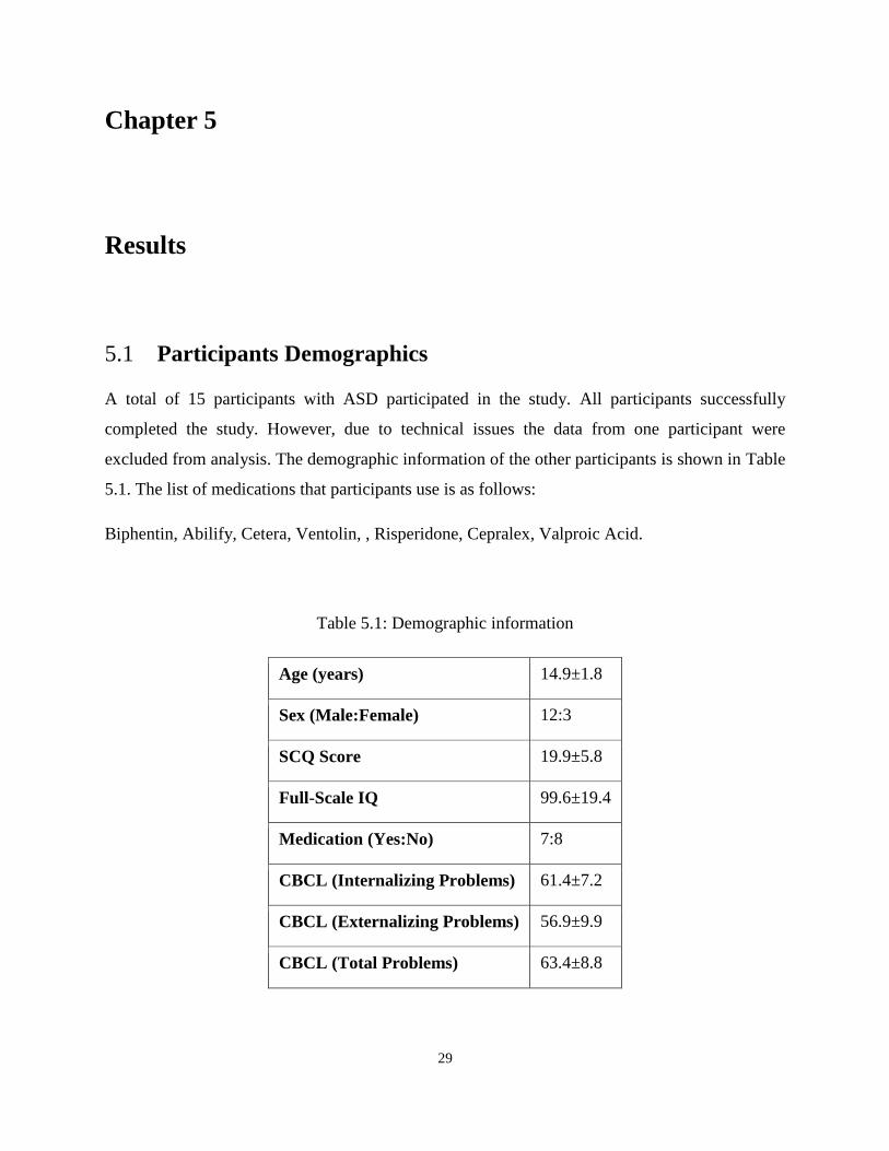
A total of 15 participants with ASD participated in the study. All participants successfully

completed the study. However, due to technical issues the data from one participant were

excluded from analysis. The demographic information of the other participants is shown in Table

5.1. The list of medications that participants use is as follows:

Biphentin, Abilify, Cetera, Ventolin, , Risperidone, Cepralex, Valproic Acid.

Table 5.1: Demographic information

Age (years) 14.9±1.8

Sex (Male:Female) 12:3

SCQ Score 19.9±5.8

Full-Scale IQ 99.6±19.4

Medication (Yes:No) 7:8

CBCL (Internalizing Problems) 61.4±7.2

CBCL (Externalizing Problems) 56.9±9.9

CBCL (Total Problems) 63.4±8.8

30

5.2 SAM Results

The results of child and parent assessments are summarized in Tables 5.2, 5.3, and 5.4. These

results were obtained after dichotomizing the valence into positive and negative as well as the

arousal into high and low. As seen in general there is poor agreement between ratings. The only

exception is agreement between child’s ratings and actual label for positive stimuli.

Table 5.2: Overall SAM results for each participant

Agreement (%)

Participant Child & Actual Parent & Actual Child & Parent

1 25 25 0

2 37.5 0 37.5

3 25 37.5 25

4 37.5 12.5 37.5

5 25 37.5 12.5

6 50 25 12.5

7 37.5 0 0

8 0 25 0

9 0 12.5 25

10 25 25 12.5

11 25 25 0

12 25 25 37.5

13 12.5 12.5 12.5

14 25 25 0

Mean 25±13.9 20.5±11.6 15.2±14.9

Table 5.3: Emotion specific SAM results for each participant

31

Agreement between child & actual labels (%)

participant Low High Positive Negative

1 100 0 100 0

2 0 100 100 75

3 50 25 75 75

4 25 50 75 100

5 0 75 100 25

6 75 100 75 50

7 25 100 100 25

8 25 0 50 25

9 25 0 100 0

10 50 25 75 100

11 25 75 100 25

12 75 0 75 50

13 100 0 0 50

14 75 0 100 25

Mean 46.4±33.8 39.3±42.4 80.4±28.0 44.6±32.8

Table 5.4: Emotion specific SAM results for each parent

Agreement between parent and actual labels (%)

Participant Low High Positive Negative

1 25 75 50 25

2 0 25 75 50

3 25 100 50 75

4 25 0 50 50

5 100 50 100 0

6 50 25 100 50

32

7 0 25 0 0

8 75 0 25 50

9 25 25 50 75

10 25 75 50 75

11 50 25 25 25

12 75 75 25 50

13 100 0 50 25

14 75 50 25 50

Mean 46.4±33.8 39.3±32.1 48.2±28.5 42.9±24.9

Tables 5.5 and 5.6 demonstrate confusion matrix for children and parents assessing high and low

arousal as well as positive and negative valence. Errors were due to negative stimuli being rated

as positive and positive ones being assessed as negative. As it can be seen, for both parent and

child the number of mislabeled pictures for high stimuli is slightly more than low stimuli.

Regarding valence, for parent the error is comparable between two cases; however, children

assessed positive pictures more correctly than negative ones.

Table 5.5: Confusion matrix for child SAM ratings

Child choice

n=112 High Low Neutral

Actual

labels

High 22 25 9

Low 18 26 12

Child choice

n=112 Positive Negative Neutral

Actual

labels

Positive 45 2 9

Negative 18 25 13

33

Table 5.6: Confusion matrix for parent SAM ratings

Parent choice

n=112 High Low Neutral

Actual

labels

High 22 25 9

Low 15 27 14

Parent choice

n=112 Positive Negative Neutral

Actual

labels

Positive 27 17 12

Negative 19 24 13

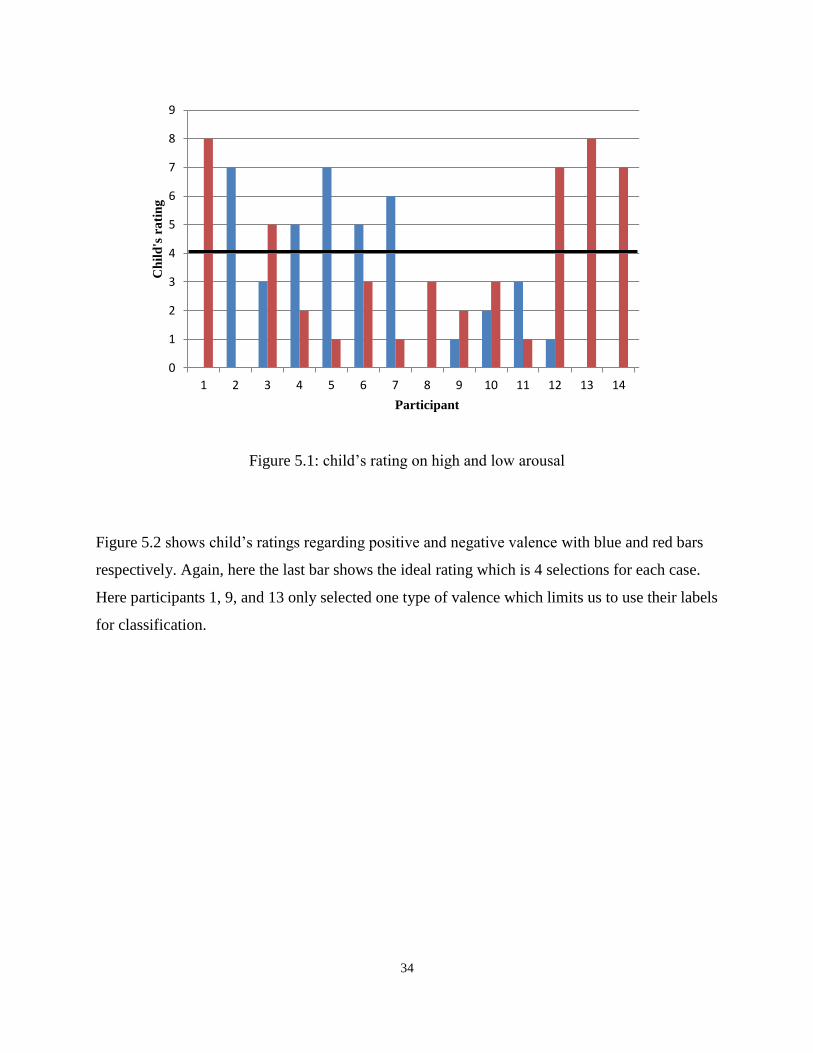
Figure 5.1 shows child’s ratings on high and low arousal. The blue and red bars denote high and

low arousal respectively. The horizontal black bar indicates the desirable case in which both

arousal and valence are selected equally 4 times as it was intended. It can be found that for none

of the participants ratings are balanced. In 5 cases (participants 1, 2, 8, 13, and 14) we only have

one bar instead of two which means that the child only has selected one type of arousal (i.e.

either high or low). This restricts us from using their labels for classification as two different

labels are required for two classes.

34

Figure 5.1: child’s rating on high and low arousal

Figure 5.2 shows child’s ratings regarding positive and negative valence with blue and red bars

respectively. Again, here the last bar shows the ideal rating which is 4 selections for each case.

Here participants 1, 9, and 13 only selected one type of valence which limits us to use their labels

for classification.

0

1

2

3

4

5

6

7

8

9

1 2 3 4 5 6 7 8 9 10 11 12 13 14 15

Ch

ild

's r

ati

ng

Participant

35

Figure 5.2: child’s rating on positive and negative valence

5.3 Classification Results

Tables 5.7 and 5.8 represent classification accuracy for each classifier in comparison of high

arousal/positive valence vs. high arousal/negative valence, and low arousal/positive valence vs.

low arousal/negative valence respectively. The results are not significantly different for various

classifiers as examined by rank sum test.

Table 5.7: Accuracy of comparing HP vs. HN for each classifier

High/positive vs. high/negative (%)

Participant KNN3 KNN5 KNN7 LDA SVML SVM poly SVM rbf

1 74.2 74.2 73.3 77.3 74.4 75 74.4

2 55.8 54.4 55.6 58.8 54.8 60.4 59.2

3 59.4 53.1 55 62.3 61.5 63.1 53.3

4 90.6 91 90.6 88.3 89.6 91.7 91

0

1

2

3

4

5

6

7

8

9

1 2 3 4 5 6 7 8 9 10 11 12 13 14 15

Ch

ild

's r

ati

ng

Participants

36

5 71 69.2 66.7 61.7 63.1 64 69

6 49 47.7 47.9 49.4 45.6 48.1 50.2

7 76.7 75.2 74 80 68.1 77.7 77.7

8 85.4 87.5 86.9 89.2 84 87.3 87.7

9 71.3 70.4 70.6 66.3 57.5 66.5 69.8

10 63.3 63.3 62.3 69.6 53.5 63.8 62.3

11 75.2 75 74.4 78.1 76.3 80.6 80.8

12 74.8 73.5 73.1 71.9 72.1 73.5 71.9

13 68.3 69.4 68.8 71.7 68.3 71.7 70.2

14 73.5 74.8 75.4 71.5 70.8 74 72.5

Mean 70.6±11.0 69.9±12.2 69.6±11.7 71.1±11.1 67.1±12.1 71.2±11.4 70.7±11.8

Table 5.8: Accuracy of comparing LP vs. LN

Low/positive vs. low/negative (%)

Participant KNN3 KNN5 KNN7 LDA SVML SVM poly SVM rbf

1 75.8 74.6 74.0 87.5 66.7 74.8 76.3

2 84.8 85.2 84.4 85.4 86.0 85.4 85.4

3 90.4 89.8 88.3 90.8 90.8 92.5 90.6

4 74.0 73.8 72.9 77.5 74.2 81.0 76.7

5 80.2 80.0 80.4 76.9 77.5 81.3 80.8

6 49.6 55.2 52.9 61.5 61.7 63.1 43.8

7 90.8 89.8 88.8 83.3 81.3 82.9 92.3

8 85.4 85.2 86.9 88.5 86.7 86.5 85.6

9 74.4 74.6 76.9 78.3 77.5 76.9 74.0

10 68.5 69.2 65.4 70.6 67.1 70.4 72.5

11 58.5 59.2 57.9 60.8 57.3 57.7 56.5

12 95.6 95.2 97.5 96.5 95.8 96.3 97.3

13 89.0 89.0 87.3 93.1 89.4 94.4 88.8

14 65.0 64.0 62.3 67.1 66.5 67.5 67.3

37

Mean 77.3±13.4 77.5±12.4 76.8±13.2 79.9±11.5 77.0±11.9 79.3±11.7 77.7±14.6

5.4 Ensemble of Classifiers

To improve outcome the classification outputs were combined using weighted majority vote as

described earlier. Table 5.9 summarizes the classification results of ensemble of methods for two

classification problems as well as maximum accuracy obtained from individual classifiers.

Although the average result is improved by combining classifiers, rank sum test showed that it is

not significantly different from the maximum distinct result.

Table 5.9: Classification results of ensemble of methods

Participant

Accuracy

(%) HP vs.

HN

Max accuracy of HP

vs. HN for individual

classifiers(%)

Accuracy

(%) LP vs.

LN

Max accuracy of LP

vs. LN for individual

classifiers(%)

1 81.2 77.3 86.1 87.5

2 75.8 60.4 85.1 86.0

3 73.8 63.1 95.0 92.5

4 93.8 91.7 82.5 81.0

5 79.6 71.0 87.9 81.3

6 70.5 50.2 73.9 63.1

7 87.4 80.0 92.2 92.3

8 91.0 89.2 90.7 88.5

9 83.5 71.3 79.8 78.3

10 84.8 69.6 78.3 72.5

11 83.4 80.8 71.8 60.8

12 77.8 74.8 97.9 97.5

13 80.4 71.7 90.3 94.4

38

14 78.1 75.4 79.4 67.5

Mean 81.5±6.4 73.3±10.9 85.1±7.8 81.7±11.8

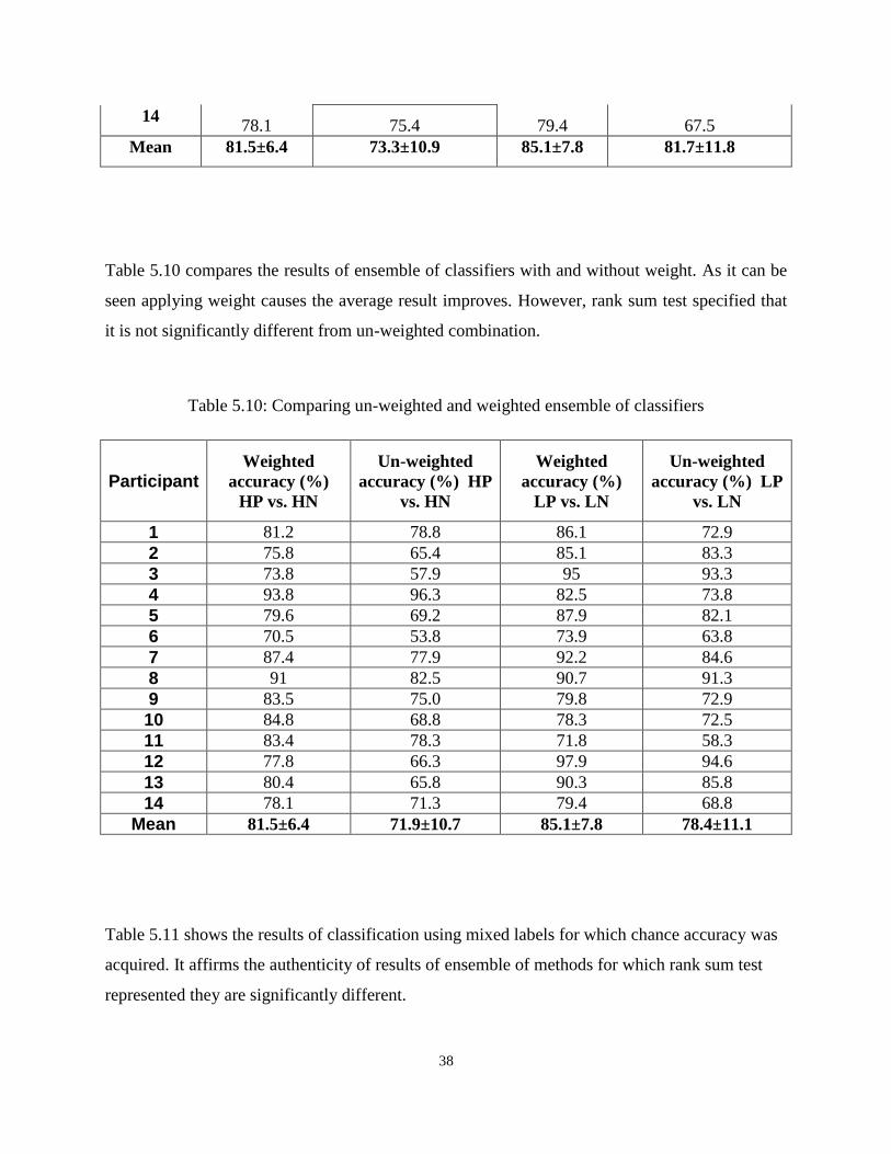
Table 5.10 compares the results of ensemble of classifiers with and without weight. As it can be

seen applying weight causes the average result improves. However, rank sum test specified that

it is not significantly different from un-weighted combination.

Table 5.10: Comparing un-weighted and weighted ensemble of classifiers

Participant Weighted

accuracy (%)

HP vs. HN

Un-weighted

accuracy (%) HP

vs. HN

Weighted

accuracy (%)

LP vs. LN

Un-weighted

accuracy (%) LP

vs. LN

1 81.2 78.8 86.1 72.9

2 75.8 65.4 85.1 83.3

3 73.8 57.9 95 93.3

4 93.8 96.3 82.5 73.8

5 79.6 69.2 87.9 82.1

6 70.5 53.8 73.9 63.8

7 87.4 77.9 92.2 84.6

8 91 82.5 90.7 91.3

9 83.5 75.0 79.8 72.9

10 84.8 68.8 78.3 72.5

11 83.4 78.3 71.8 58.3

12 77.8 66.3 97.9 94.6

13 80.4 65.8 90.3 85.8

14 78.1 71.3 79.4 68.8

Mean 81.5±6.4 71.9±10.7 85.1±7.8 78.4±11.1

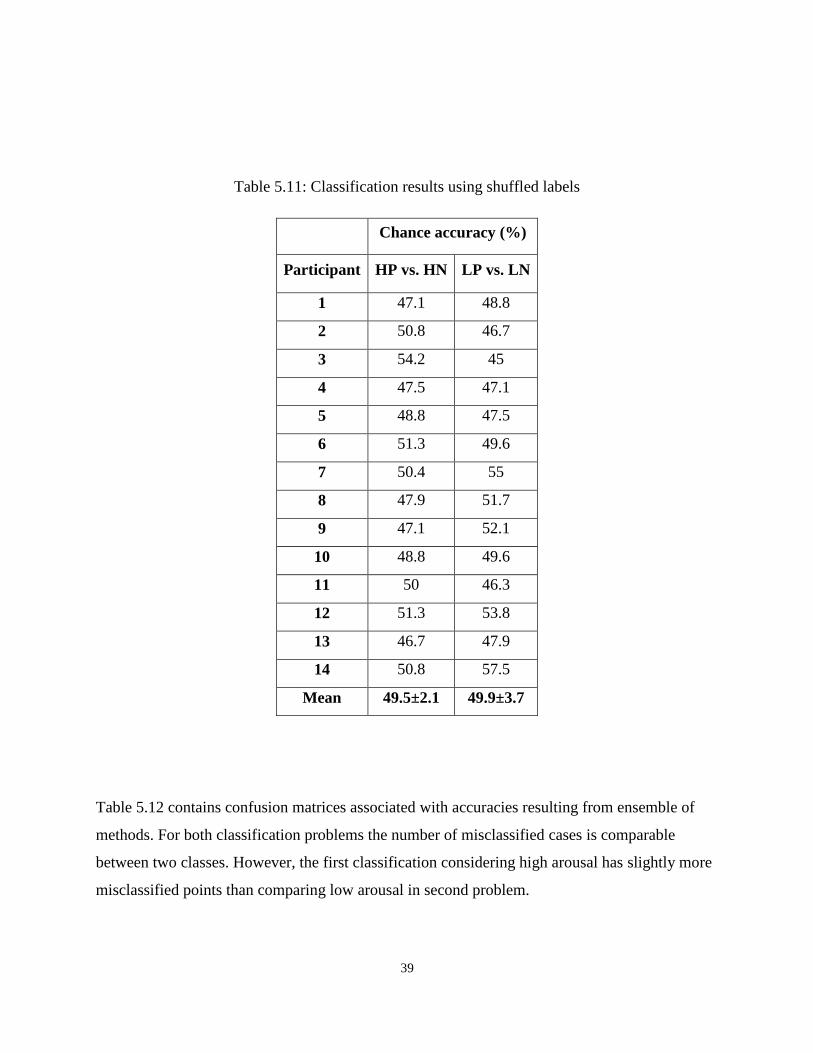
Table 5.11 shows the results of classification using mixed labels for which chance accuracy was

acquired. It affirms the authenticity of results of ensemble of methods for which rank sum test

represented they are significantly different.

39

Table 5.11: Classification results using shuffled labels

Chance accuracy (%)

Participant HP vs. HN LP vs. LN

1 47.1 48.8

2 50.8 46.7

3 54.2 45

4 47.5 47.1

5 48.8 47.5

6 51.3 49.6

7 50.4 55

8 47.9 51.7

9 47.1 52.1

10 48.8 49.6

11 50 46.3

12 51.3 53.8

13 46.7 47.9

14 50.8 57.5

Mean 49.5±2.1 49.9±3.7

Table 5.12 contains confusion matrices associated with accuracies resulting from ensemble of

methods. For both classification problems the number of misclassified cases is comparable

between two classes. However, the first classification considering high arousal has slightly more

misclassified points than comparing low arousal in second problem.

40

Table 5.12: Confusion matrices of ensemble of methods

Predicted labels

n=8400 High/Negative High/Positive

Actual

labels

High/Negative 3453 747

High/Positive 853 3347

Predicted labels

n=8400 Low/Negative Low/Positive

Actual

labels

Low/Negative 3598 602

Low/Positive 613 3587

The results of two classification approaches are shown in Figure 5.3 to easier interpret. For all

participants the accuracies are above 70%. As it can be understood from the bars, there are

variations between individual results.

41

Figure 5.3: Bar plot of results of ensemble of classifiers

5.5 Classification over arousal axis

The goal of this thesis was to find patterns along valence axis as it has already been shown that

the difference between high and low arousal is detectable [13]. To examine the veracity of this

supposition we also have discriminated data in high/positive vs. low/positive as well as

high/negative vs. low/negative classes. The results are demonstrated in Table 5.13. It can be

inferred that the accuracies are considerably better than chance which confirms the possibility of

distinguishing pattern in arousal level.

Table 5.13: Discriminating high vs. low arousal

Participant HP vs. LP (%) HN vs. LN (%)

1 85.9 85.8

42

2 92.3 75.2

3 85.8 98.4

4 86.5 98.1

5 85.1 89.7

6 83.8 77.5

7 91.7 97.3

8 91.3 91.3

9 71.4 81.2

10 74.3 86.3

11 84.8 72.5

12 95.2 84.5

13 75.6 91.8

14 85.8 79.1

Mean 85.0±6.7 86.3±8.2

5.6 Modality Specific Results

To investigate the effect of physiological modality on the final results classification was

performed using features of each signal separately. Table 5.14 sums up the sensor specific results

of ensemble of classifiers. Rank sum test has indicated that there is no significant difference

between the results of each sensor.

Table 5.14: Signal specific results, SC: Skin Conductance, Resp: Respiration, Temp:

Temperature

High/positive vs. high/negative Low/positive vs. low/negative

Par ECG SC Resp Temp All

sensors ECG SC Resp Temp

All

sensors

1 72.3 87.1 71.7 77.7 81.2 92.1 76 73.5 72.9 86.1

2 74.8 71 81.5 76.7 75.8 70.8 85.2 83.5 76.3 85.1

3 76.5 75 73.5 75.8 73.8 89.8 77.3 95.6 79.6 95

4 70 88.8 84.6 71.9 93.8 75.8 81.5 97.7 70 82.5

5 72.3 83.3 76.3 78.8 79.6 67.9 82.1 70.6 78.5 87.9

6 74.6 70.8 73.3 73.3 70.5 74.6 69.6 70.8 74.2 73.9

7 71.5 98.1 82.1 73.3 87.4 75.2 80 79.4 96.7 92.2

8 72.7 78.3 73.1 77.3 91 74.2 92.3 76.7 73.3 90.7

9 74.6 76.9 74.4 88.1 83.5 82.5 77.9 76.3 74.6 79.8

43

10 76.3 74 83.3 80 84.8 72.5 71.3 74.2 71.9 78.3

11 74.4 85.4 73.8 75.4 83.4 80.4 72.7 70 73.3 71.8

12 69.8 73.5 73.1 85.8 77.8 75.2 99.4 75.2 73.3 97.9

13 75.6 70.8 83.5 76.3 80.4 99.2 75.8 96.7 69.4 90.3

14 71.9 75.4 80.2 72.9 78.1 74 70.4 76 78.5 79.4

Mean 73.4±2.2 79.2±8.2 77.5±4.8 77.4±4.7 81.5±6.4 78.9±9.0 79.4±8.5 79.7±9.8 75.9±6.7 85.1±7.8

We ran the classification for each modality without feature selection. As can be seen in Figure

5.4 the accuracies for all the participants, except one result for participant 4, are above 70%.

Figure 5.4: Accuracy results with full feature set for each signal

5.7 Selected Features

A histogram of selected features for two classification methods is demonstrated in Figure 5.5. As

the figure shows, average SC signal is the most frequent selected signal followed by average

temperature in both cases. There is no feature that is not selected at any time.

44

Figure 5.5: Selected features, RR-int: RR intervals of ECG, HR: heart rate, RI: respiration

intervals, RR: respiration rate, Resp: respiration, Temp: temperature, SCR: skin conductance

response

Top ten features for each classification problem are listed in Table 5.15. Features from all four

sensors are among the most selected features.

Table 5.15: Top ten selected features

Feature ranking HP vs. HN LP vs. LN

45

1 Mean SC Mean SC

2 Mean temperature Mean temperature

3 Minimum temperature Minimum respiration rate

4 Minimum respiration rate Mean RR interval

5 Standard deviation of temperature Mean temperature

6 Slope of SC signal Standard deviation respiration interval

7 Mean respiration interval Minimum respiration interval

8 Slope of temperature signal Mean respiration rate

9 Mean respiration rate Maximum RR interval

10 Minimum respiration interval Slope of temperature

Figure 5.6 includes heat maps indicating selected features for each participant in low arousal,

high arousal, and subtraction of low from high arousal respectively. The numbers on each plot

signify the number of times the feature was selected in 100 runs of classification.

46

(a) Frequency of selecting each feature in classifying low/positive vs. low/negative

47

(b) Frequency of selecting each feature in classifying high/positive vs. high/negative

48

(c) Difference of frequency of feature selection in two classification problems

Figure 5.6: Frequency of feature selection for each participant for: (a) low arousal, (b) high

arousal, (c) subtracting a from b. The numbers on the plot show the number of times each feature

is selected out of 100 runs of classification

49

5.9 Association of Classification Accuracy and SAM Ratings with

Demographics

We conducted linear regression analysis to examine the effect of demographic information on

classification accuracy. The results are summarized in Tables 5.16 (a) and (b). As it is indicated

age, gender, IQ, and CBCL scores do not have significant effect on classification accuracy.

However, SCQ score has significant effect on accuracy in comparison high/positive vs.

high/negative states. We may not detect effects for other demographics due to inadequate power

caused by limited sample size. Figure 5.7 demonstrates the scatter plot of accuracy results of

classifying high/positive vs. high/negative against SCQ score. It indicates that the higher SCQ

score, the lower accuracy.

Table 5.16: Effect of demographic information on classification accuracy

Regression slope Standard Error t-stat P-value

Age 1.116 0.998 1.119 0.285

Gender -3.720 4.231 -0.879 0.397

IQ 0.116 0.086 1.353 0.201

SCQ -0.889 0.216 -4.118 0.001*

CBCL-Internalizing problems -0.236 0.249 -0.949 0.361

CBCL-Externalizing problems 0.175 0.182 0.963 0.354

(a) Effect of demographic information on classification results of high/positive vs. high/negative


Age 0.717 1.257 0.570 0.579

Gender 3.750 5.192 0.722 0.484

IQ 0.003 0.112 0.027 0.979

SCQ 0.519 0.379 1.370 0.196



50

(b) Effect of demographic information on classification results of low/positive vs. low/negative

Figure 5.7: Accuracy of classifying HP vs. HN against SCQ scores

Tables 5.17 (a) to (d) show the effect of demographics on the results of consistency of children’s

rating with actual labels. As can be seen, none of the parameters has significant effect on the

results. Agaian, we may not be able to detect the effects due to small power because of limited

sample size.

Table 5.17: Effect of demographic information on SAM results


Age -5.245 5.286 -0.992 0.341

51

Gender 15.152 22.469 0.674 0.513

IQ -0.343 0.474 -0.722 0.484

SCQ 0.663 1.749 0.379 0.711


CBCL-Externalizing problems -1.841 0.833 -2.210 0.047

(a) Effect of demographic information on results of consistency of child’s ratings and actual labels for

stimuli with low arousal


Age 3.234 6.844 0.473 0.645

Gender 34.848 26.941 1.294 0.220

IQ -0.914 0.548 -1.666 0.122

SCQ 1.298 2.179 0.596 0.562

CBCL-Internalizing problems 1.190 1.664 0.715 0.488

CBCL-Externalizing problems -0.641 1.228 -0.522 0.611

(b) Effect of demographic information on results of consistency of child’s ratings and actual labels for

stimuli with high arousal


Age -7.430 4.031 -1.843 0.090

Gender 3.788 18.980 0.200 0.845

IQ -0.267 0.395 -0.677 0.511

SCQ 1.137 1.424 0.799 0.440



(c) Effect of demographic information on results of consistency of child’s ratings and actual labels for

stimuli with positive valence


Age 4.983 5.141 0.969 0.352

Gender -3.788 22.199 -0.171 0.867

IQ 0.381 0.457 0.834 0.421

52

SCQ -1.012 1.683 -0.601 0.559



(d) Effect of demographic information on results of consistency of child’s ratings and actual labels for

stimuli with negative valence

5.10 Effect of Window Size on Accuracy

Figures 5.8 and 5.9 indicate the effect of window size in which features are extracted to be used

in classification as data points on the performance of classifiers. Each bar denotes accuracy of

ensemble of methods for one specific segmentation. Different window lengths are listed in Table

5.18. As examined by rank sum test there is no significant difference between various cases.

Figure 5.8: Results of various segmentations in classifying LP vs. LN

53

Figure 5.9: Results of various segmentations in classifying HP vs. HN

Table 5.18: Data partitioning

Segmentation Length of train:test (sec) Sub-window size (sec) Shift (sec)

1 320:160 30 15

2 320:160 20 15

3 360:120 20 15

4 320:160 30 10

5 320:160 20 10

6 360:120 20 10

7 320:160 30 5

8 320:160 20 5

9 360:120 20 5

54

Chapter 6

Discussion and Conclusion

6.1 SAM assessment

Overall, the results of our study revealed poor agreement between child/parent assessments of

emotional stimuli and the true labels as well as between child and parent assessments. The results

of child assessments are not supervising given the known difficulties with emotion processing

and recognition in ASD [6]. We did not find a significant effect of age or IQ on assessment

agreement, indicating that the discrepancy is not likely due to misunderstanding the task. There

was also no effect of symptom severity, measured by the SCQ, on assessment agreement.

Interestingly, when looking at the results per emotion type, we found that there was a high

agreement between child SAM reports and actual labels for the positive stimuli. These results

suggest a bias toward interpretation of negative stimuli in ASD [75], a finding consistent with

existing reports in the literature.

The differences in recognition accuracy between positive and negative emotions may also be

related to an imbalance in the stimuli potency between negative and positive stimuli. In

particular, we excluded highly negative stimuli from our picture selection as these were

inappropriate for child viewing. There was such restriction for erotic pictures in positive stimuli

while there were suitable alternatives in other themes for them.

Our results also show poor agreement between parent assessments and actual labels as well as

child labels. Anecdotally, several parents reported that they were unable to discern their

children’s reactions during the study as overt expressions were minimal.

55

6.2 Feature selection

We employed an automatic feature selection algorithm to reduce the number of features for

classification. This algorithm chooses a subset of features that maximize classification accuracy.

As such, the results of feature selection can provide insight into the usefulness of each feature to

differentiating between the emotional responses. Our results show that features from each

individual sensor (ECG, SC, respiration, and temperature) provide viable features for

classification with over 70% accuracy for the two classification problems considered herein. In

addition, mean SC was the most frequently selected feature for classification across all

participants.

SC signal receives inputs only from sympathetic branch of ANS while other signals have input

of both sympathetic and parasympathetic nervous system [76]. It may be related to the fact SC

reflects emotional states better than other signals as it is stimulated more specifically. Our results

also show that combining features across sensors improves average classification accuracies. It

can be due to existence of complimentary information in the separated signals.

Comparing the selected features for each participants, it is evidence that although some features

are more frequently selected across participants overall, the subset of optimal features is person-

dependent. This is consistent with reports of person stereotypy – that is, for each individual, the

autonomic response to stimuli may exhibit different, but reproducible, levels of activity in each

physiological measure [77].

Differences in selected features may also be related to varying quality of data recorded from each

sensor for different participants. Differences in data quality may have results from differences in

sensor positioning and adhesion, or varying degrees of noise (e.g., participant) affecting each

sensor. An important implication of our findings is that classification algorithms should focus on

individual participants instead of considering groups.

Usability purposes make it essential to reach an integrated set of features for each participant as

in the real world it is not efficient to select the optimum set of features in each circumstance. In

this regard classification was performed using the data of each signal at a time without feature

selection. The accuracy results are above 70% in all the cases except in one participant for one of

56

the signals. This finding suggests that even if we consider one signal and use the genuine

features we still obtain an acceptable result better than chance.

6.3 Classification Results

Overall, our results indicate that positive and negative affective states can be automatically

differentiated with accuracies greater than 80%. In this study, the average of accuracy in

differentiating of differently valenced states was higher under low arousal conditions as

compared to high arousal. This may be related to the potency of the stimuli as was shown in the

ratings of selected stimuli. For instance, for low positive emotion elicitation the average of

valence is 8.1 while for high positive it is 6.91 (the closer to 9, the more positive). The level of

arousal is 2.16 and 5.38 for the first and second stimuli respectively which implies the former

one is close enough to low arousal as it supposed to be while the later one is close to neutral

whereas it is intended to be high arousal.

To investigate whether the difference in the classification results is due to masking the valence

patterns by arousal, the pattern recognition was also performed to distinguish variations in

arousal level (comparing high/positive vs. low/positive and high/negative vs. low/negative). The

average of the results is also higher than 80% in these two cases. It can be inferred that the data

shows pattern in both arousal and valence dimensions.

As specified in table 5.10 classification results of ensemble of methods in general is higher than

individual classifiers. Using ensemble of classifiers boosted the average classification accuracy.

The best obtained accuracy for single classifiers was 79.9% and 71.2% respectively for

comparing low/positive vs. low/negative and high/positive vs. high negative. The accuracy

increased to 85.1% and 81.5% respectively by combining classifiers which is 5.2% improvement

for the first and 10.3% for the second case.

For all participants in comparison of high/positive vs. high/negative states and for 12 cases out of

14 participants in discriminating low/positive vs. low/negative the combination of classifiers

outperformed the maximum result achieved by a single method. In those two cases that it did not

57

enhance the accuracy, the results were comparable (the accuracies were 86.3% and 85.8% for

combined model, and 87.5% and 86.0% for maximum result of separate methods respectively. It

was also shown that weighted majority vote has performed better than simple majority vote. It is

attributable to the fact that in weighted model methods with higher performance receive greater

weight than the ones acted poorly while in simple majority vote all the methods have equal effect

on the final result.

Confusion matrices in table 5.13 shows the number of correctly classified points between

high/positive and high/negative emotions as well as low/positive and low/negative ones are

relatively similar, indicating that the classifier is not biased towards any of the classes.

According to bar plot of various methods of segmentation, partitioning order number 9 for which

the number of obtained data points is slightly higher than the other cases acquired better results.

As it was aforementioned the intended labels were decided to be used in the analyses. Three

possible scenarios can be considered: 1- The child’s labels are similar to intended labels. As it

was shown it is not the case in this study. 2- The child’s labels are different from actual labels

and the latter one is correct. It was what we assumed here and obtained acceptable accuracy for

classification. 3- The child’s labels and intended labels are different and the former is the right

label. To test this hypothesis we tried to use child’s ratings for classification. As it was shown in

Figures 5.1 and 5.2 the labels prevented us from performing classification as for several

participants we only had one type of label, while two distinct labels are required for pattern

analysis. Therefore, testing this case was impossible in this study.

6.4 Effect of demographic variables/behavioural measures on

accuracy

According to Figure 5.5 (e), SCQ score has significant effect on the result of discriminating

high/positive vs. high/negative emotions and the higher SCQ score, the lower accuracy of

classification. This effect can stem from different reasons. SCQ score is a representation of

severity of autism. Higher SCQ implies less ability in perceiving stimuli intended influence, and

therefore not discriminating between various emotional states effectively. It also can cause

58

variations in physiological signals so that the changes may not be clearly distinguishable for each

affective state.

Age, IQ, gender, and CBCL score do not have any significant effect on the results. This implies

that possibility of finding patterns in physiological data in various affective states is similar for

all participants regardless of these three specifications. It is also possible that we have not

detected effects for other demographics due to inadequate power caused by limited sample size.

59

Chapter 7

Conclusion

In this study the feasibility of differentiating physiological signals of children with ASD in four

emotional classes namely, high/positive, high/negative, low/positive, and low/negative was

investigated. 15 participants with ASD completed the task of watching pictures as stimuli to

elicit targeted emotions. The pictures were selected from gold standard collections which were

used in several related studies before. After collecting physiological signals using four sensors

including ECG, EDA, temperature, and respiration, pre-processing was done to remove artifacts

from the data. Then various statistical features in the time domain were extracted from each

signal. As the number of features was high compared to number of data points, feature selection

was performed using sequential forward selection, backward elimination. Then, Seven

classification methods comprise of KNN with K equal to 3, 5, and 7; LDA; SVM Linear, SVM

with polynomial kernel (order 3), and SVM with Radial Basis Function were combined using

weighted majority vote. The intended labels were considered for classification due to severe

mismatch between ratings of participants and parents with actual labels. The results suggest that

there is distinguishable pattern in the signals between aforementioned classes as supported by

average classification accuracies of 81.0% for comparing high/positive vs. high/negative and

84.9% for discriminating low/positive vs. low/negative. It was also indicated that the result of

ensemble of methods had higher performance than individual classifiers. It acted significantly

better chance which supports its validity.

The outcome of this research was a physiological approach to detection of emotions which can

provide a language-free, non-invasive, and low-cost way for characterization of emotional states

in children with ASD. This work can ultimately contribute to improving self-awareness of

emotions by providing users with information regarding their actual body state. In addition it will

enhance our understanding of ASD-related emotion processing difficulties.

60

The limitations on the way of this study included: 1- being ethically restricted in choosing

powerful stimuli. 2- Short length of measured signals which impacted the quality and amount of

extractable information; for instance, frequency features were not suitable to be obtained for this

signal size. 3- Sample size was small implying that applying some algorithms is unfavorable. As

an example, finding subgroups of individuals in different measures can be done on a larger

sample sizes.

In future, the sample size can be increased to enable performing clustering to find subgroups of

similar individuals. Also, a group of typical participants can be added for comparison purposes

and investigating whether or not detecting patterns in the physiological signals is better

achievable in one group than the other. Lastly, the design of study can be changed to multiple

visits of each participant to have longer duration of data recording which increases the amount of

information.

61

References

[1] American Psychiatric Association. Diagnostic and statistical manual of mental disorders,

text revision (DSM-IV-TR). American Psychiatric Association, 2000.

[2] Honkalampi, K., Hintikka, J., Tanskanen, A., Lehtonen, J., & Viinamäki, H. (2000).

Depression is strongly associated with alexithymia in the general population. Journal of

psychosomatic research, 48(1), 99-104.

[3] Baron-Cohen, S. E., Tager-Flusberg, H. E., & Cohen, D. J. (1994). Understanding other

minds: Perspectives from autism. In Most of the chapters in this book were presented in draft

form at a workshop in Seattle, Apr 1991. Oxford University Press.

[4] Frith, U. (2004). Emanuel Miller lecture: Confusions and controversies about Asperger

syndrome. Journal of child psychology and psychiatry, 45(4), 672-686.

[5] Baron-Cohen, S., Lombardo, M., Tager-Flusberg, H., & Cohen, D. (Eds.). (2013).

Understanding Other Minds: Perspectives from developmental social neuroscience. OUP

Oxford.

[6] Silani, G., Bird, G., Brindley, R., Singer, T., Frith, C., & Frith, U. (2008). Levels of

emotional awareness and autism: an fMRI study. Social neuroscience, 3(2), 97-112.

[7] Sifneos, Peter E. "The prevalence of'alexithymic'characteristics in psychosomatic patients."

Psychotherapy and psychosomatics 22 (1973): 255-62.

[8] Linden, W., Wen, F., & Paulhus, D. L. (1995). Measuring alexithymia: reliability, validity,

and prevalence. Advances in personality assessment, 10, 51-95.

[9] Hill, Elisabeth, Sylvie Berthoz, and Uta Frith. "Brief report: Cognitive processing of own

emotions in individuals with autistic spectrum disorder and in their relatives." Journal of autism

and developmental disorders 34, no. 2 (2004): 229-235.

62

[10] Bachevalier, J., & Loveland, K. A. (2006). The orbitofrontal–amygdala circuit and self-

regulation of social–emotional behavior in autism. Neuroscience & Biobehavioral Reviews,

30(1), 97-117.

[11] Lambie, J. A., & Marcel, A. J. (2002). Consciousness and the varieties of emotion

experience: a theoretical framework. Psychological review, 109(2), 219.

[12] Shalom, D. Ben, S. H. Mostofsky, R. L. Hazlett, M. C. Goldberg, R. J. Landa, Y. Faran, D.

R. McLeod, and R. Hoehn-Saric. "Normal physiological emotions but differences in expression

of conscious feelings in children with high-functioning autism." Journal of autism and

developmental disorders 36, no. 3 (2006): 395-400.

[13] Kushki, Azadeh, Ajmal Khan, Jessica Brian, and Evdokia Anagnostou. "A Kalman

Filtering Framework for Physiological Detection of Anxiety-Related Arousal in Children with

Autism Spectrum Disorder." (2014).

[14] Kennedy, Daniel P., Elizabeth Redcay, and Eric Courchesne. "Failing to deactivate: resting

functional abnormalities in autism." Proceedings of the National Academy of Sciences 103, no.

21 (2006): 8275-8280.

[15] Rieffe, C., Terwogt, M. M., & Kotronopoulou, K. (2007). Awareness of single and multiple

emotions in high-functioning children with autism. Journal of autism and developmental

disorders, 37(3), 455-465.

[16] Picard, R. W., Vyzas, E., & Healey, J. (2001). Toward machine emotional intelligence:

Analysis of affective physiological state. Pattern Analysis and Machine Intelligence, IEEE

Transactions on, 23(10), 1175-1191.

[17] Liu, Changchun, Karla Conn, Nilanjan Sarkar, and Wendy Stone. "Physiology-based affect

recognition for computer-assisted intervention of children with Autism Spectrum Disorder."

International journal of human-computer studies 66, no. 9 (2008): 662-677.

[18] Baltaxe, Christiane AM, and James Q. Simmons III. "Prosodic development in normal and

autistic children." In Communication problems in autism, pp. 95-125. Springer US, 1985.

63

[19] Luu, Sheena, and Tom Chau. "Decoding subjective preference from single-trial near-

infrared spectroscopy signals." Journal of neural engineering 6, no. 1 (2009): 016003.

[20] Kandel, Eric R., James H. Schwartz, and Thomas M. Jessell, eds. Principles of neural

science. Vol. 4. New York: McGraw-Hill, 2000.

[21] Andreassi, John L. Psychophysiology: Human behavior & physiological response.

Psychology Press, 2000.

[22] Nasoz, Fatma, Christine L. Lisetti, Kaye Alvarez, and Neal Finkelstein. "Emotion

recognition from physiological signals for user modeling of affect." In Proceedings of the 3rd

Workshop on Affective and Attitude User Modelling (Pittsburgh, PA, USA. 2003.

[23] Ekman, Paul, Wallace V. Friesen, Maureen O'Sullivan, Anthony Chan, Irene Diacoyanni-

Tarlatzis, Karl Heider, Rainer Krause et al. "Universals and cultural differences in the judgments

of facial expressions of emotion." Journal of personality and social psychology 53, no. 4 (1987):

712.

[24] Peter, Christian, and Antje Herbon. "Emotion representation and physiology assignments in

digital systems." Interacting with Computers 18, no. 2 (2006): 139-170.

[25] Lang, Peter J. "The emotion probe: studies of motivation and attention." American

psychologist 50, no. 5 (1995): 372.

[26] Hamann, Stephan. "Mapping discrete and dimensional emotions onto the brain:

controversies and consensus." Trends in cognitive sciences 16, no. 9 (2012): 458-466.

[27] Wilson-Mendenhall, Christine D., Lisa Feldman Barrett, and Lawrence W. Barsalou.

"Neural evidence that human emotions share core affective properties." Psychological science

24, no. 6 (2013): 947-956.

[28] Barrett, Lisa Feldman, and Eliza Bliss‐Moreau. "Affect as a psychological primitive."

Advances in experimental social psychology 41 (2009): 167-218.

64

[29] Jerritta, S., Murugappan, M., Nagarajan, R., & Wan, K. (2011, March). Physiological

signals based human emotion recognition: a review. In Signal Processing and its Applications

(CSPA), 2011 IEEE 7th International Colloquium on (pp. 410-415). IEEE.

[30] Lang, Peter J., Margaret M. Bradley, and Bruce N. Cuthbert. "International affective picture

system (IAPS): Affective ratings of pictures and instruction manual." Technical report A-8

(2008).

[31] Rigas, G., Katsis, C. D., Ganiatsas, G., & Fotiadis, D. I. (2007). A user independent,

biosignal based, emotion recognition method. In User Modeling 2007 (pp. 314-318). Springer

Berlin Heidelberg.

[32] Haag, A., Goronzy, S., Schaich, P., & Williams, J. (2004, June). Emotion recognition using

bio-sensors: First steps towards an automatic system. In ADS (pp. 36-48).

[33] Maaoui, C., Pruski, A., & Abdat, F. (2010). Emotion recognition through physiological

signals for human-machine communication. INTECH Open Access Publisher.

[34] Gu, Y., Tan, S. L., Wong, K. J., Ho, M. H. R., & Qu, L. (2010, July). A biometric signature

based system for improved emotion recognition using physiological responses from multiple

subjects. In Industrial Informatics (INDIN), 2010 8th IEEE International Conference on (pp. 61-

66). IEEE.

[35] Gross, James J., and Robert W. Levenson. "Emotion elicitation using films." Cognition &

Emotion 9, no. 1 (1995): 87-108.

[36] Nasoz, F., Alvarez, K., Lisetti, C. L., & Finkelstein, N. (2004). Emotion recognition from

physiological signals using wireless sensors for presence technologies. Cognition, Technology &

Work, 6(1), 4-14.

[37] Li, L., & Chen, J. H. (2006, December). Emotion recognition using physiological signals

from multiple subjects. In Intelligent Information Hiding and Multimedia Signal Processing,

2006. IIH-MSP'06. International Conference on (pp. 355-358). IEEE.

65

[38] Wan-Hui, W., Yu-Hui, Q., & Guang-Yuan, L. (2009, March). Electrocardiography

recording, feature extraction and classification for emotion recognition. In Computer Science and

Information Engineering, 2009 WRI World Congress on (Vol. 4, pp. 168-172). IEEE.

[39] Kim, Jonghwa, and Elisabeth André. "Emotion recognition based on physiological changes

in music listening." Pattern Analysis and Machine Intelligence, IEEE Transactions on 30, no. 12

(2008): 2067-2083.

[40] Wagner, J., Kim, J., & André, E. (2005, July). From physiological signals to emotions:

Implementing and comparing selected methods for feature extraction and classification. In

Multimedia and Expo, 2005. ICME 2005. IEEE International Conference on (pp. 940-943).

IEEE.

[41] Cheng, B., & Liu, G. Y. (2008, May). Emotion recognition from surface EMG signal using

wavelet transform and neural network. In Proceedings of The 2nd International Conference on

Bioinformatics and Biomedical Engineering (ICBBE) (pp. 1363-1366).

[42] Zhu, X. (2010, April). Emotion recognition of EMG based on BP neural network. In Proc

Int Symposium Network. Network Security (pp. 227-229).

[43] Kim, Jonghwa. Bimodal emotion recognition using speech and physiological changes.

INTECH Open Access Publisher, 2007.

[44] Kim, Kyung Hwan, S. W. Bang, and S. R. Kim. "Emotion recognition system using short-

term monitoring of physiological signals." Medical and biological engineering and computing

42, no. 3 (2004): 419-427.

[45] Kushki, Azadeh, Ellen Drumm, Michele Pla Mobarak, Nadia Tanel, Annie Dupuis, Tom

Chau, and Evdokia Anagnostou. "Investigating the autonomic nervous system response to

anxiety in children with autism spectrum disorders." PLoS one 8, no. 4 (2013): e59730.

[46] Kootz, John P., and Donald J. Cohen. "Modulation of sensory intake in autistic children:

Cardiovascular and behavioral indices." Journal of the American Academy of Child Psychiatry

20, no. 4 (1981): 692-701.

66

[47] Jansen, Lucres Mc, Christine C. Gispen-de Wied, Rutger-Jan van der Gaag, and Herman

van Engeland. "Differentiation between autism and multiple complex developmental disorder in

response to psychosocial stress." Neuropsychopharmacology: official publication of the

American College of Neuropsychopharmacology 28, no. 3 (2003): 582-590.

[48] Groden, June, Matthew S. Goodwin, M. Grace Baron, Gerald Groden, Wayne F. Velicer,

Lewis P. Lipsitt, Stefan G. Hofmann, and Brett Plummer. "Assessing cardiovascular responses to

stressors in individuals with autism spectrum disorders." Focus on Autism and Other

Developmental Disabilities 20, no. 4 (2005): 244-252.

[49] Groden, June, Amy Diller, Margaret Bausman, Wayne Velicer, Gregory Norman, and

Joseph Cautela. "The development of a stress survey schedule for persons with autism and other

developmental disabilities." Journal of Autism and Developmental Disorders 31, no. 2 (2001):

207-217.

[50] Brown, R. Michael, Lisa R. Hall, Roee Holtzer, Stephanie L. Brown, and Norma L. Brown.

"Gender and video game performance." Sex Roles 36, no. 11-12 (1997): 793-812.

[51] Pecchinenda, Anna. "The affective significance of skin conductance activity during a

difficult problem-solving task." Cognition & Emotion 10, no. 5 (1996): 481-504.

[52] Bölte, S., Feineis-Matthews, S., & Poustka, F. (2008). Brief report: Emotional processing in

high-functioning autism—physiological reactivity and affective report. Journal of Autism and

Developmental Disorders, 38(4), 776-781.

[53] Kim, Kyung Hwan, S. W. Bang, and S. R. Kim. "Emotion recognition system using short-

term monitoring of physiological signals." Medical and biological engineering and computing

42, no. 3 (2004): 419-427.

[54] Brown, R. Michael, Lisa R. Hall, Roee Holtzer, Stephanie L. Brown, and Norma L. Brown.

"Gender and video game performance." Sex Roles 36, no. 11-12 (1997): 793-812.

[55] Bradley, Margaret M., and Peter J. Lang. "Emotion and motivation." Handbook of

psychophysiology 2 (2000): 602-642.

67

[56] Katsis, Christos D., Nikolaos Katertsidis, George Ganiatsas, and Dimitrios I. Fotiadis.

"Toward emotion recognition in car-racing drivers: A biosignal processing approach." Systems,

Man and Cybernetics, Part A: Systems and Humans, IEEE Transactions on 38, no. 3 (2008):

502-512.

[57] SHUSTERMAN, V, and BARNEA, O. (1995): 'Analysis of skin-temperature variability

compared to variability of blood pressure and heart rate', IEEE Ann. Conf Engineering Medicine

Biology Society, pp. 1027-1028

[58] KATAOKA, H., KANO, H., YOSHIDA, H., SAIJO, A., YASUDA, M., and OSUMI, M.

(1998): 'Development of a skin temperature measuring system for non-contact stress evaluation'.

IEEE Ann. Conf. Engineering Medicine Biology Society, pp. 940-943

[59] Peper, E., Harvey, R., Lin, I. M., Tylova, H., & Moss, D. (2007). Is there more to blood

volume pulse than heart rate variability, respiratory sinus arrhythmia, and cardiorespiratory

synchrony?. Biofeedback, 35(2).

[64] Lord, C., Risi, S., Lambrecht, L., Cook Jr, E. H., Leventhal, B. L., DiLavore, P. C., ... &

Rutter, M. (2000). The Autism Diagnostic Observation Schedule—Generic: A standard measure

of social and communication deficits associated with the spectrum of autism. Journal of autism

and developmental disorders, 30(3), 205-223.

[66] Dan-Glauser, E. S., & Scherer, K. R. (2011). The Geneva affective picture database

(GAPED): a new 730-picture database focusing on valence and normative significance. Behavior

research methods, 43(2), 468-477.

[68] Bradley, M., & Lang, P. J. (1999). The International affective digitized sounds (IADS)[:

stimuli, instruction manual and affective ratings. NIMH Center for the Study of Emotion and

Attention.

[69] Pan, J., & Tompkins, W. J. (1985). A real-time QRS detection algorithm. Biomedical

Engineering, IEEE Transactions on, (3), 230-236.

[70] Lacey, John I., and Beatrice C. Lacey. "Verification and extension of the principle of

autonomic response-stereotypy." The American journal of psychology (1958): 50-73.

68

[71] Kulic, D., & Croft, E. (2007). Affective state estimation for human–robot interaction.

Robotics, IEEE Transactions on, 23(5), 991-1000.

[72] Zong, C., & Chetouani, M. (2009, December). Hilbert-Huang transform based

physiological signals analysis for emotion recognition. In Signal Processing and Information

Technology (ISSPIT), 2009 IEEE International Symposium on (pp. 334-339). IEEE.

[73] Hönig, F., Wagner, J., Batliner, A., & Nöth, E. (2009). Classification of user states with

physiological signals: On-line generic features vs. specialized feature sets. In Proc. of the 17th

European Signal Processing Conference (EUSIPCO-2009).

[74] Faul, F., Erdfelder, E., Lang, A. G., & Buchner, A. (2007). G* Power 3: A flexible

statistical power analysis program for the social, behavioral, and biomedical sciences. Behavior

research methods, 39(2), 175-191.

[75] Ashwin, C., Chapman, E., Colle, L., & Baron-Cohen, S. (2006). Impaired recognition of

negative basic emotions in autism: A test of the amygdala theory. Social neuroscience, 1(3-4),

349-363.

[76] Boucsein, W. (2012). Electrodermal activity. Springer Science & Business Media.

[77] Lacey, J. I., & Lacey, B. C. (1958). Verification and extension of the principle of autonomic

response-stereotypy. The American journal of psychology, 71(1), 50-73.

[78] Schapire, R. E., Freund, Y., Bartlett, P., & Lee, W. S. (1998). Boosting the margin: A new

explanation for the effectiveness of voting methods. Annals of statistics, 1651-1686.

[79] Dietterich, T. G. (2000). An experimental comparison of three methods for constructing

ensembles of decision trees: Bagging, boosting, and randomization. Machine learning, 40(2),

139-157.

[80] Kuncheva, L. I., & Whitaker, C. J. (2003). Measures of diversity in classifier ensembles

and their relationship with the ensemble accuracy. Machine learning, 51(2), 181-207.

[81] Ganong, W. F., & Barrett, K. E. (1995). Review of medical physiology (pp. 474-478).

Norwalk, CT: Appleton & Lange.

69

[82] Cuthbert, B. N., Schupp, H. T., Bradley, M. M., Birbaumer, N., & Lang, P. J. (2000). Brain

potentials in affective picture processing: covariation with autonomic arousal and affective

report. Biological psychology, 52(2), 95-111.

[83] Thayer, J. F., & Lane, R. D. (2000). A model of neurovisceral integration in emotion

regulation and dysregulation. Journal of affective disorders, 61(3), 201-216.

[84] Jatupaiboon, N., Pan-ngum, S., & Israsena, P. (2013). Real-time EEG-based happiness

detection system. The Scientific World Journal, 2013.

[85] Jatupaiboon, N., Pan-ngum, S., & Israsena, P. (2013). Real-time EEG-based happiness

detection system. The Scientific World Journal, 2013.

[86] http://biosig.sourceforge.net/download.html

[87] Benedek, M., & Kaernbach, C. (2010). A continuous measure of phasic electrodermal

activity. Journal of neuroscience methods, 190(1), 80-91.

physiological detection of emotional states in children

Documents